Quality of Institutions, Technological Progress, and Pollution Havens in Latin America. An Analysis of the Environmental Kuznets Curve Hypothesis


Abstract
1. Introduction
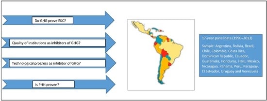
- Did Latin American Greenhouse Gas emissions prove the EKC hypothesis?
- Did the quality of institutions play a compensating role for income on environmental stress?
- Did technological progress act in line with the quality of institutions to help decouple income from environmental stress?
- Has the PHH been proven for the selected sample during the period under consideration?
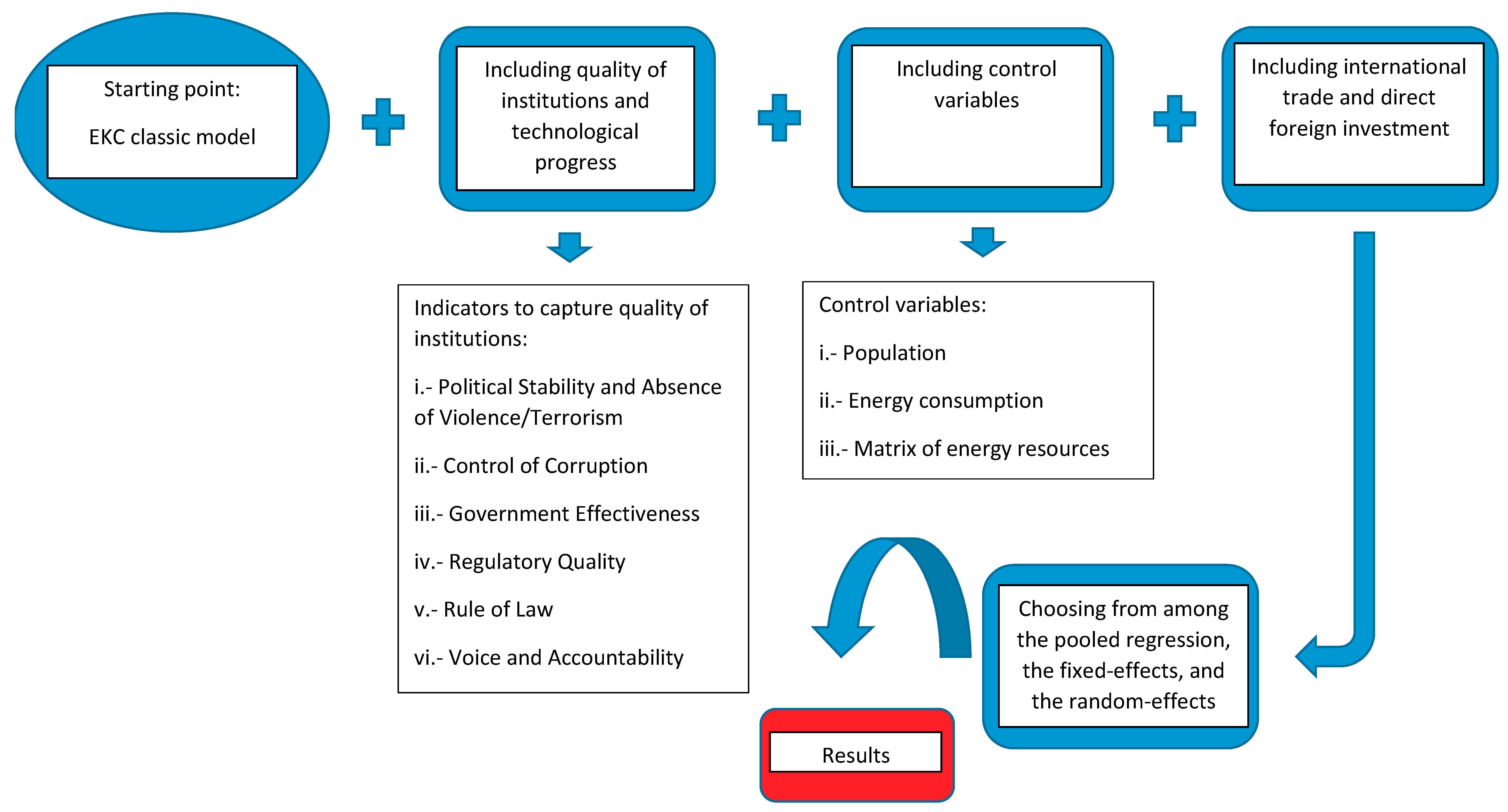
2. Materials and Methods
2.1. Methods
2.2. Data
3. Results
3.1. Model Estimation
3.2. Discussion of Major Findings
4. Conclusions
Author Contributions
Funding
Acknowledgments
Conflicts of Interest
References
- Kuznets, S. Economic Growth and Income Inequality. Am. Econ. Assoc. 1955, 45, 1–28. [Google Scholar]
- Grossman, G.M.; Krueger, A.B. Economic Growth and the Environment. Q. J. Econ. 1995, 110, 353–377. [Google Scholar] [CrossRef]
- Panayotou, T. Economic growth and the environment. In The environment in Anthropoly; Haenn, N., Wilck, R.R., Eds.; NYU Press: New York, NY, USA, 2016; pp. 140–148. [Google Scholar]
- Yandle, B.; Vijayaraghavan, M.; Bhattarai, M. The Environmental Kuznets Curve; A Primer, PERC Research Study; The Property and Environment Research Center: Bozeman, MT, USA, 2002. [Google Scholar]
- Dinda, S. Environmental Kuznets Curve Hypothesis: A Survey. Ecol. Econ. 2004, 49, 431–455. [Google Scholar] [CrossRef]
- Kaika, D.; Zervas, E. The Environmental Kuznets Curve (EKC) theory—Part A: Concept, causes and the CO2 emissions case. Energy Policy 2013, 62, 1392–1402. [Google Scholar] [CrossRef]
- Stern, D.I. The rise and fall of the environmental Kuznets curve. World Dev. 2004, 32, 1419–1439. [Google Scholar] [CrossRef]
- Panayotou, T. Demystifying the environmental Kuznets curve: Turning a black box into a policy tool. Environ. Dev. Econ. 1997, 2, 465–484. [Google Scholar] [CrossRef]
- Munasinghe, M. Is environmental degradation an inevitable consequence of economic growth: Tunneling through the environmental Kuznets curve. Ecol. Econ. 1999, 29, 89–109. [Google Scholar] [CrossRef]
- North, D.C. Institutions. J. Econ. Perspect. 1991, 5, 97–112. [Google Scholar] [CrossRef]
- OECD–Organization for Economic Co-Operation and Development 2002. Indicators to Measure Decoupling of Environmental Pressure from Economic Growth Sustainable Development. SG/SD (2002) 1/Final (2002). Available online: http://www.olis.oecd.org/olis/2002doc.nsf/LinkTo/sg-sd(2002)1-final (accessed on 25 October 2018).
- De Freitas, L.C.; Kaneko, S. Decomposing the decoupling of CO2 emissions and economic growth in Brazil. Ecol. Econ. 2011, 70, 1459–1469. [Google Scholar] [CrossRef]
- Mundaca, L. Climate change and energy policy in Chile: Up in smoke? Energy Policy 2013, 52, 235–248. [Google Scholar] [CrossRef]
- Bhattarai, M.; Hammig, M. Institutions and the Environmental Kuznets Curve for Deforestation: A Crosscountry Analysis for Latin America, Africa and Asia. World Dev. 2001, 29, 995–1010. [Google Scholar] [CrossRef]
- Culas, R.J. Deforestation and the environmental Kuznets curve: An institutional perspective. Ecol. Econ. 2007, 61, 429–437. [Google Scholar] [CrossRef]
- Bernauer, T.; Koubi, V. Effects of political institutions on air quality. Ecol. Econ. 2009, 68, 1355–1365. [Google Scholar] [CrossRef]
- Bhattacharya, M.; Awaworyi, C.S.; Paramati, S.R. The dynamic impact of renewable energy and institutions on economic output and CO2 emissions across regions. Renew. Energy 2017, 111, 157–167. [Google Scholar] [CrossRef]
- Hosseini, M.H.; Kaneko, S. Can environmental quality spread through institutions? Energy Policy 2013, 56, 312–321. [Google Scholar] [CrossRef]
- Bokpin, G.A. Foreign direct investment and environmental sustainability in Africa: The role of institutions and governance. Res. Int. Bus. Finance 2017, 39, 239–247. [Google Scholar] [CrossRef]
- Gill, F.L.; Viswanathan, K.K.; Karim, M.Z.A. The Critical Review of the Pollution Haven Hypothesis (PHH). Int. J. Energy Econ. Policy 2018, 8, 167–174. [Google Scholar]
- Leamer, E.E. Sources of International Comparative Advantage: Theory and Evidence; MIT press: Cambridge, MA, USA, 1984. [Google Scholar]
- Cole, M.A.; Elliott, R.J. FDI and the capital intensity of “dirty” sectors: A missing piece of the pollution haven puzzle. Rev. Dev. Econ. 2005, 9, 530–548. [Google Scholar] [CrossRef]
- Mabey, N.; McNally, R. Foreign Direct Investment and the Environment: from Pollution Havens to Sustainable Development; A WWF-UK Report; World Wildlife Fund: London. UK, 1999. [Google Scholar]
- De Bruyn, S. Explaining the environmental Kuznets curve: Structural change and international agreements in reducing sulphur emissions. Environ. Dev. Econ. 1997, 2, 485–503. [Google Scholar] [CrossRef]
- Pablo-Romero, M.d.P.; De Jesús, J. Economic growth and energy consumption: The Energy-Environmental Kuznets Curve for Latin America and the Caribbean. Renew. Sustain. Energy Rev. 2016, 60, 1343–1350. [Google Scholar] [CrossRef]
- Pablo-Romero, M.d.P.; Sánchez-Braza, A. Residential energy environmental Kuznets curve in the EU-28. Energy 2017, 125, 44–54. [Google Scholar] [CrossRef]
- Özokcu, S.; Özdemir, Ö. Economic growth, energy, and environmental Kuznets curve. Renew. Sustain. Energy Rev. 2017, 72, 639–647. [Google Scholar] [CrossRef]
- Liobikienė, G.; Butkus, M. Environmental Kuznets Curve of greenhouse gas emissions including technological progress and substitution effects. Energy 2017, 135, 237–248. [Google Scholar] [CrossRef]
- Sanchez, L.F.; Stern, D.I. Drivers of industrial and non-industrial greenhouse gas emissions. Ecol. Econ. 2016, 124, 17–24. [Google Scholar] [CrossRef]
- Yang, X.; Lou, F.; Sun, M.; Wang, R.; Wang, Y. Study of the relationship between greenhouse gas emissions and the economic growth of Russia based on the Environmental Kuznets Curve. Appl. Energy 2017, 193, 162–173. [Google Scholar] [CrossRef]
- Lu, W.C. Greenhouse gas emissions, energy consumption and economic growth: A panel cointegration analysis for 16 Asian countries. Int. J. Environ. Res. Public Health 2017, 14, 1436. [Google Scholar] [CrossRef]
- Yin, J.; Zheng, M.; Chen, J. The effects of environmental regulation and technical progress on CO2 Kuznets curve: An evidence from China. Energy Policy 2015, 77, 97–108. [Google Scholar] [CrossRef]
- Apergis, N.; Ozturk, I. Testing environmental Kuznets Curve hypothesis in Asian countries. Ecol. Indic. 2015, 52, 16–22. [Google Scholar] [CrossRef]
- Chang, C.P.; Hao, Y. Environmental performance, corruption and economic growth: Global evidence using a new data set. Appl. Econ. 2016, 49, 498–514. [Google Scholar] [CrossRef]
- Halkos, G.E.; Paizanos, E.A. The channels of the effect of government expenditure on the environment: Evidence using dynamic panel data. J. Environ. Plan. Manag. 2017, 60, 135–157. [Google Scholar] [CrossRef]
- Charfeddine, L.; Mrabet, Z. The impact of economic development and social-political factors on ecological footprint: A panel data analysis for 15 MENA countries. Renew. Sustain. Energy Rev. 2017, 76, 138–154. [Google Scholar] [CrossRef]
- WGI, The World Bank Group. Available online: http://info.worldbank.org/governance/wgi/#reports (accessed on 15 June 2017).
- Kaufmann, D.; Kraay, A.; Mastruzzi, M. Response to ‘What do the worldwide governance indicators measure?’. Eur. J. Dev. Res. 2010, 22, 55–58. [Google Scholar] [CrossRef]
- Cole, M.A. Trade, the pollution haven hypothesis and the environmental Kuznets curve: Examining the linkages. Ecol. Econ. 2004, 48, 71–81. [Google Scholar] [CrossRef]
- Ehrlich, P.R.; Holdren, J.P. Impact of Population Growth. Science 1971, 171, 1212–1217. [Google Scholar] [CrossRef] [PubMed]
- Commoner, B. The Closing Circle: Nature, Man, and Technology; Alfred A. Knopf: New York, NY, USA, 1971. [Google Scholar]
- Dietz, T.; Rosa, A.E. Rethinking the Environmental Impacts of Population, Affluence and Technology. Hum. Ecol. Rev. 1994, 1, 277–300. [Google Scholar]
- Dietz, T.; Rosa, A.E. Climate change and society: Speculation, construction and scientific investigation. Int. Sociol. 1998, 13, 421–455. [Google Scholar]
- Wernick, I.K.; Waggoner, P.E.; Ausubel, J.H. Searching for Leverage to Conserve Forests: The Industrial Ecology of Wood Products in the United States. J. Ind. Ecol. 1997, 1, 125–145. [Google Scholar] [CrossRef]
- Grossman, G.M.; Krueger, A.B. Environmental Impacts of a North American Free Trade Agreement; The Mexico-U.S. Free Trade Agreement, Garber, P., Eds.; MIT Press: Cambridge, MA, USA, 1993. [Google Scholar]
- Copeland, B.R.; Taylor, M.S. Trade, growth, and the environment. J. Econ. Lit. 2004, 42, 7–71. [Google Scholar] [CrossRef]
- Zhang, S.; Liu, X.; Bae, J. Does trade openness affect CO2 emissions: Evidence from ten newly industrialized countries? Environ. Sci. Pollut. Res. 2017, 24, 17616–17625. [Google Scholar] [CrossRef]
- Ozatac, N.; Gokmenoglu, K.K.; Taspinar, N. Testing the EKC hypothesis by considering trade openness, urbanization, and financial development: The case of Turkey. Environ. Sci. Pollut. Res. 2017, 24, 16690–16701. [Google Scholar] [CrossRef]
- López, L.A.; Arce, G.; Zafrilla, J.E. Parcelling virtual carbon in the pollution haven hypothesis. Energy Econ. 2013, 39, 177–186. [Google Scholar] [CrossRef]
- Xing, Y.; Kolstad, C.D. Do Lax Environmental Regulations Attract Foreign Investment? Environ. Res. Econ. 2002, 21, 1–22. [Google Scholar] [CrossRef]
- He, J. Pollution haven hypothesis and environmental impacts of foreign direct investment: The case of industrial emission of sulfur dioxide (SO2) in Chinese provinces. Ecol. Econ. 2006, 60, 228–245. [Google Scholar] [CrossRef]
- Mulatu, A. The Structure of UK Outbound FDI and Environmental Regulation. Environ. Resour. Econ. 2017, 68, 65–96. [Google Scholar] [CrossRef]
- Sun, C.; Zhang, F.; Xu, M. Investigation of pollution haven hypothesis for China: An ARDL approach with breakpoint unit root tests. J. Clean. Prod. 2017, 161, 153–164. [Google Scholar] [CrossRef]
- Liu, Y.; Hao, Y.; Gao, Y. The environmental consequences of domestic and foreign investment: Evidence from China. Energy Policy 2017, 108, 271–280. [Google Scholar] [CrossRef]
- Forslid, R.; Okubo, T.; Sanctuary, M. Trade Liberalization, Transboundary Pollution, and Market Size. J. Assoc. Environ. Resour. Econ. 2017, 4, 927–957. [Google Scholar] [CrossRef]
- Hoffman, R.; Sing, L.C.; Ramasamy, B.; Yeung, M. FDI and pollution: A granger causality test using panel data. J. Int. Dev. 2005, 17, 311–317. [Google Scholar] [CrossRef]
- Kentor, J.; Boswell, T. Foreign capital dependence and development: A new direction. Am. Sociol. Rev. 2003, 68, 301–313. [Google Scholar] [CrossRef]
- Jorgenson, A.K. Does foreign investment harm the air we breathe and the water we drink? A cross-national study of carbon dioxide emissions and organic water pollution in less-developed countries 1975–2000. Organ. Environ. 2007, 20, 137–156. [Google Scholar] [CrossRef]
- Jorgenson, A.K. Foreign direct investment and the environment, the mitigating influence of institutional and civil society factors, and relationship between industrial pollution and human health: A panel study of less-developed countries. Organ. Environ. 2009, 22, 135–157. [Google Scholar] [CrossRef]
- Jorgenson, A.K. The transnational organization of production, the scale of degradation: And eco efficiency: A study of carbon dioxide emissions in less-developed countries. Hum. Ecol. Rev. 2009, 16, 64–74. [Google Scholar]
- Kanemoto, K.; Moran, D.; Lenzen, M.; Geschke, A. International trade undermines national emission reduction targets: New evidence from air pollution. Glob. Environ. Chang. 2014, 24, 52–59. [Google Scholar] [CrossRef]
- Pesaran, M.H. General Diagnostic Tests for Cross Section Dependence in Panels; Cambridge Working Papers WP0435; Faculty of Economics University of Cambridge: Cambridge, UK, 2004. [Google Scholar]
- Breusch, T.; Pagan, A. The Lagrange multiplier and its applications to model specificatión in econometrics. Rev. Econ. Stud. 1980, 47, 239–253. [Google Scholar] [CrossRef]
- Hausman, J.A. Specification test in econometrics. Econometrica 1978, 46, 1251–1271. [Google Scholar] [CrossRef]
- Hausman, J.; McFadden, C. Specification test in econometrics. Econometrica 1984, 52, 1219–1240. [Google Scholar] [CrossRef]
- Greene, W.H. Econometric Analysis, 7th ed.; Stern School of Business New York University: Pearson, London, UK, 2012. [Google Scholar]
- Wooldridge, J. Econometric Analysis of Cross Section and Panel Data; MIT Press: Cambridge, MA, USA, 2002. [Google Scholar]
- Beck, N. Time-Series-Cross-Section Data: What have we learned in the past few years? Ann. Rev. Polit. Sci. 2001, 4, 271–293. [Google Scholar] [CrossRef]
- Al-Mulali, U.; Tang, C.F.; Ozturk, I. Estimating the environment Kuznets curve hypothesis: Evidence from Latin America and the Caribbean countries. Renew. Sustain. Energy Rev. 2015, 50, 918–924. [Google Scholar] [CrossRef]
- Zilio, M.; Recalde, M. GDP and environment pressure: The role of energy in Latin America and the Caribbean. Energy Policy 2011, 39, 7941–7949. [Google Scholar] [CrossRef]
- Martinez-Zarzoso, I.; Bengochea, A. Testing for an Environmental Kuznets Curve in Latin-American Countries. Rev. Anal. Econ. 2003, 18, 2003. [Google Scholar]
- Zhou, Y.; Zhu, S.; He, C. How do environmental regulations affect industrial dynamics? Evidence from China’s pollution-intensive industries. Habitat Int. 2017, 60, 10–18. [Google Scholar] [CrossRef]
- Shen, J.; Wei, Y.D.; Yang, Z. The impact of environmental regulations on the location of pollution-intensive industries in China. J. Clean. Prod. 2017, 148, 785–794. [Google Scholar] [CrossRef]
- Migration Policy Institute, n.d. Available online: https://www.migrationpolicy.org/regions/south-america (accessed on 22 October 2018).
- Smarzynska, B.; Wei, S.J. Pollution Havens and Foreign Direct Investment: Dirty Secret or Popular Myth? Working Papers 8465; National Bureau of Economic Research: Cambridge, MA, USA, 2005. [Google Scholar]
- Eskeland, G.; Harrison, A. Moving to greener pastures? Multinationals and the pollution-haven hypothesis. J. Dev. Econ. 2003, 70, 1–23. [Google Scholar] [CrossRef]
- Dean, J.M.; Lovely, M.E.; Wang, H. Foreign Direct Investment and Pollution Havens: Evaluating the Evidence from China; Working Paper N° 2004-01-B U.S. International Trade Commission: Washington, DC, USA, 2002. [Google Scholar]
- Kearsley, A.; Riddel, M. A further inquiry into the Pollution Haven Hypothesis and the Environmental Kuznets Curve. Ecol. Econ. 2010, 69, 905–919. [Google Scholar] [CrossRef]
- Sapkota, P.; Bastola, U. Foreign direct investment, income, and environmental pollution in developing countries: Panel data analysis of Latin America. Energy Econ. 2017, 64, 206–212. [Google Scholar] [CrossRef]
- Rafindadi, A.A.; Muye, I.M.; Kaita, R.A. The effects of FDI and energy consumption on environmental pollution in predominantly resource-based economies of the GCC. Sustain. Energy Technol. Assess. 2018, 25, 126–137. [Google Scholar] [CrossRef]


| > 0 | = 0 | = 0 | Monotonically increasing |
| < 0 | = 0 | = 0 | Monotonically decreasing |
| > 0 | < 0 | = 0 | Inverted U shape. The EKC is valid. |
| < 0 | > 0 | = 0 | U Shape |
| > 0 | < 0 | > 0 | N form |
| < 0 | > 0 | < 0 | Inverted N shape |
| Variable | Explanation | Unit | Source | Expected Sign |
|---|---|---|---|---|
| ln (GHGpc) | Total greenhouse gas emission | ln (kt of CO2 equivalent) | WDI | |
| ln (GDPpc) | GDP per capita, PPP (current international $) | ln (1000 US$ 2011) | WDI | Positive |
| GDP per capita square | WDI | Negative | ||
| GDP per capita cube | WDI | ± | ||
| PSAVT | Political Stability and Absence of Violence/Terrorism (PSAVT) | Values between −2.5 and 2.5 | WGI | Negative |
| CC | Control of Corruption (CC) | Values between −2.5 and 2.5 | WGI | Negative |
| GE | Government Effectiveness (GE) | Values between −2.5 and 2.5 | WGI | Negative |
| RQ | Regulatory Quality (RQ) | Values between −2.5 and 2.5 | WGI | Negative |
| RL | Rule of Law (RL) | Values between −2.5 and 2.5 | WGI | Negative |
| VA | Voice and Accountability (VA) | Values between −2.5 and 2.5 | WGI | Negative |
| TECH | High-technology exports | Percentage of manufactured exports | WGI | Negative |
| ln(GDPpc) × PSAVT/CC/GE/RQ/RL/VA | Terms of interaction | Positive | ||
| × PSAVT/CC/GE/RQ/RL/VA | Terms of interaction | Negative | ||
| × PSAVT/CC/GE/RQ/RL/VA | Terms of interaction | ± | ||
| ln(GDPpc) × TECH | Terms of interaction | Positive | ||
| × ECH | Terms of interaction | Negative | ||
| × TECH | Terms of interaction | ± | ||
| Ln (P) | Total population | ln (units) | WDI | Positive |
| EC | Energy consumption (EC) per million dollars of GDP at constant 2010 prices | Thousands of barrels of oil equivalent | CEPAL | Positive. |
| EE | Renewable energy sources on total energy use | Proportion | CEPAL | Negative |
| TRADE | Merchandise trade (% of GDP) | Percentage | WDI | Positive |
| FDI | Foreign direct investment, net inflows | Percentage | WDI | Positive |
| Variable | Mean | Std. Dev. | Min | Max | Obs | |
|---|---|---|---|---|---|---|
| ln (GHGpc) | Overall | −5.330286 | 0.7015173 | −6.432259 | −2.786832 | N = 324 |
| Between | 0.6852661 | −6.265535 | −3.959671 | n = 18 | ||
| Within | 0.2173756 | −6.287268 | −4.157447 | T = 18 | ||
| ln (GDPpc) | Overall | 8.972472 | 0.5152072 | 7.738997 | 10.02322 | N = 324 |
| Between | 0.4667575 | 8.093602 | 9.559566 | n = 18 | ||
| Within | 0.2429863 | 8.480332 | 9.562592 | T = 18 | ||
| PSAVT | Overall | −0.3426055 | 0.6530893 | −2.3857 | 0.9973063 | N = 324 |
| Between | 0.6386092 | −1.749541 | 0.7633462 | n = 18 | ||
| Within | 0.2004201 | −1.062043 | 0.1544409 | T = 18 | ||
| CC | Overall | −0.303594 | 0.6779242 | −1.444359 | 1.572951 | N = 324 |
| Between | 0.6782205 | −1.124076 | 1.444894 | n = 18 | ||
| Within | 0.1542978 | −0.7346453 | 0.2069996 | T = 18 | ||
| GE | Overall | −0.2242938 | 0.5613994 | −1.195942 | 1.285714 | N = 324 |
| Between | 0.5595473 | −0.9695299 | 1.206711 | n = 18 | ||
| Within | 0.1362154 | −0.627603 | 0.2027976 | T = 18 | ||
| RQ | Overall | 0.0139563 | 0.6209773 | −1.624753 | 1.64474 | N = 324 |
| Between | 0.5780686 | −0.9828321 | 1.473358 | n 18 | ||
| Within | 0.2627492 | −0.627965 | 1.0229 | T = 18 | ||
| RL | Overall | −0.4673229 | 0.6504213 | −1.812253 | 1.374353 | N = 324 |
| Between | 0.6450485 | −1.288491 | 1.248214 | n = 18 | ||
| Within | 0.1698815 | −0.9910853 | 0.0704554 | T = 18 | ||
| VA | Overall | 0.1005125 | 0.501417 | −0.9618688 | 1.243549 | N = 324 |
| Between | 0.4887367 | −0.5652662 | 1.018083 | n = 18 | ||
| Within | 0.1585155 | −0.3783807 | 0.6263118 | T = 18 | ||
| TECH | Overall | 8.431279 | 10.28533 | 0.0013268 | 63.40368 | N = 324 |
| Between | 9.000392 | 2.104588 | 39.17926 | n = 18 | ||
| Within | 5.389303 | −26.54516 | 46.34956 | T = 18 | ||
| EC | Overall | 1.132556 | 0.4396158 | 0.5684226 | 2.250259 | N = 324 |
| Between | 0.4349587 | 0.6260214 | 1.945453 | n = 18 | ||
| Within | 0.1184493 | 0.7483654 | 1.454636 | T = 18 | ||
| EE | Overall | 32.94112 | 19.09179 | 7.208523 | 76.0548 | N = 324 |
| Between | 19.16819 | 8.317099 | 72.74032 | n = 18 | ||
| Within | 4.05148 | 20.42738 | 56.42065 | T = 18 | ||
| ln (P) | Overall | 16.43776 | 1.136914 | 14.84329 | 19.1349 | N = 324 |
| Between | 1.165363 | 15.00335 | 19.04008 | n = 18 | ||
| Within | 0.0773366 | 16.23665 | 16.62771 | T = 18 | ||
| FDI | Overall | 3.712267 | 2.771048 | −5.007236 | 16.22949 | N = 324 |
| Between | 1.969363 | 0.6969128 | 8.315166 | n = 18 | ||
| Within | 2.00111 | −3.94247 | 11.62659 | T = 18 | ||
| TRADE | Overall | 52.11963 | 23.94042 | 12.29259 | 120.7539 | N = 324 |
| Between | 20.743 | 18.93556 | 108.3071 | n = 18 | ||
| Within | 12.86537 | 14.95344 | 93.1011 | T = 18 |
| (1) | (2) | (3) | (4) | (5) | (6) | (7) | (8) | (9) | (10) | (11) | (12) | (13) | (14) | |
|---|---|---|---|---|---|---|---|---|---|---|---|---|---|---|
| (1) ln (GHGpc) | 1 | |||||||||||||
| (2) ln (GDP) | 0.26 | 1 | ||||||||||||
| (3) PSAVT | 0.01 | 0.24 | 1 | |||||||||||
| (4) CC | 0.06 | 0.45 | 0.64 | 1 | ||||||||||
| (5) GE | 0.07 | 0.49 | 0.59 | 0.90 | 1 | |||||||||
| (6) RQ | −0.16 | 0.22 | 0.51 | 0.79 | 0.86 | 1 | ||||||||
| (7) RL | 0.07 | 0.39 | 0.73 | 0.93 | 0.89 | 0.83 | 1 | |||||||
| (8) VA | 0.09 | 0.46 | 0.82 | 0.85 | 0.82 | 0.70 | 0.91 | 1 | ||||||
| (9) TECH | 0.04 | 0.10 | 0.27 | 0.25 | 0.25 | 0.21 | 0.29 | 0.37 | 1 | |||||
| (10) EC | 0.06 | −0.72 | −0.31 | −0.59 | −0.65 | −0.53 | −0.55 | −0.59 | −0.23 | 1 | ||||
| (11) EE | −0.18 | −0.47 | 0.10 | −0.06 | −0.21 | 0.02 | −0.03 | −0.04 | 0.02 | 0.40 | 1 | |||
| (12) ln (P) | 0.23 | 0.37 | −0.38 | −0.04 | 0.08 | −0.02 | −0.15 | −0.18 | 0.04 | −0.31 | −0.42 | 1 | ||
| (13) FDI | −0.06 | 0.07 | 0.32 | 0.33 | 0.38 | 0.44 | 0.43 | 0.37 | 0.13 | −0.12 | −0.08 | −0.22 | 1 | |
| (14) TRADE | −0.30 | −0.29 | 0.15 | −0.13 | −0.15 | −0.08 | −0.06 | −0.04 | 0.07 | 0.39 | 0.30 | −0.50 | 0.26 | 1 |
| (1) PSAVT | (2) CC | (3) GE | (4) RQ | (5) RL | (6) VA | |
|---|---|---|---|---|---|---|
| ΔLN (GDPPC) | 0.344 *** | 0.253 *** | 0.138 *** | 0.219 *** | 0.172 *** | 0.209 *** |
| (0.036) | (0.052) | (0.041) | (0.031) | (0.0140) | (0.022) | |
| ΔLN (GDPpc2) | −0.124 *** | −0.091 *** | −0.008 | −0.017 | −0.082 *** | −0.082 *** |
| (0.031) | (0.024) | (0.022) | (0.014) | (0.0148) | (0.015) | |
| ΔLNST | −0.081 *** | −0.140 *** | −0.033 ** | −0.042 *** | 0.025 *** | −0.074 *** |
| (0.007) | (0.011) | (0.014) | (0.010) | (0.0026) | (0.009) | |
| ΔTECH | −0.002 *** | −0.001 *** | −0.003 *** | −0.002 *** | −0.002 *** | −0.002 *** |
| (0.000) | (0.000) | (0.000) | (0.000) | (0.0001) | (0.000) | |
| ΔLN (GDP) *INST | 0.039 ** | 0.074 *** | −0.126 *** | −0.096 *** | 0.076 *** | 0.221 *** |
| (0.018) | (0.019) | (0.022) | (0.018) | (0.0090) | (0.014) | |
| ΔLN (GDP2) *INST | −0.084 *** | −0.012 | −0.048 ** | 0.093 *** | −0.043 *** | −0.008 |
| (0.022) | (0.023) | (0.022) | (0.022) | (0.0098) | (0.021) | |
| ΔLN (GDP) *TECH | −0.003 *** | −0.004 *** | −0.004 *** | −0.003 *** | −0.003 *** | −0.004 *** |
| (0.001) | (0.001) | (0.001) | (0.001) | (0.0004) | (0.001) | |
| ΔLN (GDP2) *TECH | 0.010 *** | 0.009 *** | 0.010 *** | 0.009 *** | 0.010 *** | 0.011 *** |
| (0.001) | (0.002) | (0.001) | (0.001) | (0.0005) | (0.001) | |
| ΔEC | 0.068 *** | 0.072 *** | 0.098 *** | 0.063 *** | 0.074 *** | 0.075 *** |
| (0.018) | (0.020) | (0.014) | (0.018) | (0.0045) | (0.013) | |
| ΔEE | −0.004 *** | −0.005 *** | −0.005 *** | −0.005 *** | −0.005 *** | −0.005 *** |
| (0.000) | (0.000) | (0.000) | (0.000) | (0.0001) | (0.000) | |
| ΔLN (P) | −0.384 ** | −0.057 | −0.461 *** | −0.586 *** | 0.018 | −0.177 |
| (0.158) | (0.253) | (0.095) | (0.112) | (0.0786) | (0.125) | |
| ΔFDI | −0.009 *** | −0.010 *** | −0.010 *** | −0.010 *** | −0.011 *** | −0.009 *** |
| (0.001) | (0.000) | (0.000) | (0.001) | (0.0002) | (0.000) | |
| ΔTRADE | −0.001 *** | −0.001 *** | −0.001 *** | −0.002 *** | −0.001 *** | −0.001 *** |
| (0.000) | (0.000) | (0.000) | (0.000) | (0.0001) | (0.000) | |
| WALD CHI2(30) | 2,854,429 | 1,545,303 | 4,573,330 | 2,857,421 | 75,600,000 | 429,000,000 |
| PROB > CHI2 | 0.0000 | 0.0000 | 0.0000 | 0.0000 | 0.0000 | 0.0000 |
| OBS | 306 | 306 | 306 | 306 | 306 | 306 |
| (1) PSAVT | (2) CC | (3) GE | (4) RQ | (5) RL | (6) VA | |
|---|---|---|---|---|---|---|
| ΔLN (GDPPC) | 0.406 *** | 0.370 *** | 0.256 *** | 0.318 *** | 0.263 *** | 0.393 *** |
| (0.038) | (0.069) | (0.042) | (0.042) | (0.048) | (0.053) | |
| ΔLN (GDPpc2) | −0.126 *** | 0.006 | −0.007 | 0.018 | −0.025 | 0.006 |
| (0.030) | (0.036) | (0.030) | (0.029) | (0.030) | (0.035) | |
| ΔLN (GDPpc3) | −0.231 *** | −0.178 *** | −0.140 *** | −0.154 *** | −0.133 *** | −0.162 *** |
| (0.040) | (0.043) | (0.029) | (0.030) | (0.039) | (0.037) | |
| ΔLNST | −0.107 *** | −0.130 *** | −0.056 *** | −0.053 *** | 0.007 | −0.131 *** |
| (0.008) | (0.019) | (0.013) | (0.012) | (0.013) | (0.023) | |
| ΔTECH | −0.001 *** | −0.001 | −0.002 *** | −0.002 *** | −0.002 *** | −0.002 ** |
| (0.000) | (0.001) | (0.001) | (0.000) | (0.000) | (0.001) | |
| ΔLN (GDP) *TECH | 0.061 *** | 0.185 | −0.165 *** | −0.053 *** | 0.036 | 0.540 *** |
| (0.018) | (0.034) | (0.026) | (0.024) | (0.033) | (0.046) | |
| ΔLN (GDP2) *INST | −0.072 *** | 0.060 *** | −0.006 | 0.141 *** | 0.000 | 0.156 *** |
| (0.018) | (0.028) | (0.024) | (0.025) | (0.021) | (0.040) | |
| ΔLN (GDP3) *INST | −0.063 ** | −0.111 | 0.057 * | −0.078 *** | −0.005 | −0.591 *** |
| (0.028) | (0.036) | (0.034) | (0.032) | (0.034) | (0.057) | |
| ΔLN (GDP) *TECH | 0.010 *** | −0.002 *** | 0.005 *** | −0.001 | 0.002 | −0.002 |
| (0.001) | (0.003) | (0.002) | (0.002) | (0.002) | (0.003) | |
| ΔLN (GDP2) *TECH | 0.007 *** | 0.007 *** | 0.008 *** | 0.008 *** | 0.009 *** | 0.009 *** |
| (0.001) | (0.002) | (0.001) | (0.001) | (0.001) | (0.002) | |
| ΔLN (GDP3) *TECH | −0.019 *** | −0.002 *** | −0.013 *** | −0.004 | −0.010 *** | −0.006 |
| (0.002) | (0.004) | (0.003) | (0.003) | (0.003) | (0.004) | |
| ΔEC | 0.037** | 0.060 *** | 0.092 *** | 0.055 *** | 0.072 *** | 0.056 *** |
| (0.018) | (0.026) | (0.013) | (0.014) | (0.014) | (0.020) | |
| ΔEE | −0.005 *** | −0.005 *** | −0.005 *** | −0.004 *** | −0.004 *** | −0.004 *** |
| (0.000) | (0.001) | (0.000) | (0.000) | (0.000) | (0.001) | |
| ΔLN (P) | −0.449 *** | −0.404 *** | −0.668 *** | −1.088 *** | −0.725 * | −0.658 |
| (0.137) | (0.223) | (0.149) | (0.320) | (0.391) | (0.558) | |
| ΔFDI | −0.009 *** | −0.009 *** | −0.010 *** | −0.010 *** | −0.010 *** | −0.007 *** |
| (0.000) | (0.001) | (0.000) | (0.001) | (0.001) | (0.001) | |
| ΔTRADE | −0.002 *** | −0.001 *** | −0.001 *** | −0.001 *** | −0.001 *** | −0.001 *** |
| (0.000) | (0.000) | (0.000) | (0.000) | (0.000) | (0.000) | |
| WALD CHI2(33) | 5,526,160 | 169,000,000 | 1,210,087 | 6,954,258 | 4,969,125 | 9,365,484 |
| PROB > CHI2 | 0.0000 | 0.0000 | 0.0000 | 0.0000 | 0.0000 | 0.0000 |
| OBS | 306 | 306 | 306 | 306 | 306 | 306 |
© 2019 by the authors. Licensee MDPI, Basel, Switzerland. This article is an open access article distributed under the terms and conditions of the Creative Commons Attribution (CC BY) license (http://creativecommons.org/licenses/by/4.0/).
Share and Cite
Cansino, J.M.; Román-Collado, R.; Molina, J.C. Quality of Institutions, Technological Progress, and Pollution Havens in Latin America. An Analysis of the Environmental Kuznets Curve Hypothesis. Sustainability 2019, 11, 3708. https://doi.org/10.3390/su11133708
Cansino JM, Román-Collado R, Molina JC. Quality of Institutions, Technological Progress, and Pollution Havens in Latin America. An Analysis of the Environmental Kuznets Curve Hypothesis. Sustainability. 2019; 11(13):3708. https://doi.org/10.3390/su11133708
Chicago/Turabian StyleCansino, José M., Rocio Román-Collado, and Juan C. Molina. 2019. "Quality of Institutions, Technological Progress, and Pollution Havens in Latin America. An Analysis of the Environmental Kuznets Curve Hypothesis" Sustainability 11, no. 13: 3708. https://doi.org/10.3390/su11133708
APA StyleCansino, J. M., Román-Collado, R., & Molina, J. C. (2019). Quality of Institutions, Technological Progress, and Pollution Havens in Latin America. An Analysis of the Environmental Kuznets Curve Hypothesis. Sustainability, 11(13), 3708. https://doi.org/10.3390/su11133708