The Impact of High-Speed Rail on Housing Prices: Evidence from China’s Prefecture-Level Cities

Abstract

The rapid development of the high-speed rail (HSR) network enhanced the regional accessibility between cities, drove the rise in cities’ investment levels, and expanded the activity radius of the labor force, causing changes in housing prices along the rail lines. Based on panel data of 285 cities in China from 2008–2016, this study used the difference-in-difference based on propensity score matching (PSM-DID) method to calculate the impact of HSR on housing prices. The conclusions of the study indicated that, at the regional level, HSR significantly promoted the rise in housing prices in HSR cities along the rail line. HSR had a positive effect on housing prices, where the coefficient of HSR influence was 0.1511 and passed a 1% significance test. From the perspective of the combination of sub-regional and sub-city scales, HSR mainly played a significant role in promoting housing prices in “small and medium-sized cities” and “central and western cities”, especially in small and medium-sized cities in the central and western regions; in general, HSR can narrow the housing price gap between “small and medium-sized HSR cities” in the central and western regions and large HSR cities in the east region. Lastly, the results of the intermediary mechanism test showed that the income level of residents and employment levels played an intermediary role in the influence of HSR on the housing prices of cities along the rail line. Thus, this paper suggests that the Chinese government needs to formulate housing price control policies that suit local conditions according to the characteristics of different cities.

1. Introduction

As a key promotion target of China’s “the Belt and Road” policy, high-speed rail (HSR) received extensive attention across the world. As of 2018, China became the country with the longest HSR mileage (131,000 km) in the world [1]. By 2017, China basically formed a “four vertical and four horizontal HSR network”. On 13 July 2016, the National Development and Reform Commission, the Ministry of Transport, and the China Railway Corporation jointly issued the “Mid-to-Long-Term Plan for Railway Network (2016–2030)” [2], which proposed the “eight vertical and eight horizontal HSR network”, as shown in Figure 1. Additionally, it stated that, by 2025, the scale of the railway network will reach approximately 175,000 km, including approximately 38,000 km of HSR. With the rapid development of HSR, the impact of HSR on the social and economic development of cities became the focus of attention at home and abroad. It not only attracted the attention of the government but was also very popular among scholars. Previous studies on the impact of HSR on cities along the rail line concentrated on specific aspects. Firstly, in terms of the impact of HSR on the regional economy, most scholars demonstrated that the changes in spatiotemporal structure brought about by HSR significantly drove the development of cities along the rail line [3]. HSR triggered the accumulation of urban industrial belts and industrial clusters [4]. HSR also promoted the development of regional economic integration [5]. Secondly, in terms of the employment effect of HSR, most studies showed that HSR could alter the labor force structure and ultimately improve the job market [6]. By studying the impact of European HSR construction on the spatial layout of enterprises, Vickerman [7] believed that the construction of HSR significantly promoted economic development along the rail line and improved the local employment level. Zheng and Kahn [8] discovered that HSR services enabled residents to live and work in different cities. Research by Tierney [9] showed that the construction of HSR could help form a corridor for employment, housing, and innovation. Individuals and enterprises were more densely arranged around the site, driving the employment development of the site city. Dong and Zhu [10] discovered that HSR could promote the employment level and labor mobility in cities along the route. However, some literature suggested that, for enterprises with fixed workplaces, the operation of HSR did not bring about a large employment growth effect [11]. In addition, some studies analyzed the impact of HSR on urban tourism development [12] and knowledge spillovers [13].

In terms of the impact of HSR on housing prices, most research topics focused on the impact of a single HSR on housing prices from a micro perspective. Most studies were based on the micro price data of cities along the line, using the hedonic feature price (hedonic) model for empirical analysis. Geng et al. [14] used the hedonic model to analyze the impact of HSR sites on Beijing’s housing prices, and the conclusions were significantly positive. Chen and Haynes [15] constructed a hedonic pricing model, taking the cities along the Beijing–Shanghai HSR as the research object, and discovered that HSR construction has a significant impact on urban housing prices. In summary, there are few studies on the impact of HSR on housing prices. In terms of research object, scholars mostly only studied the impact of one HSR line on urban housing prices. Most research methods involved the hedonic pricing model proposed by Rosen [16]. This method controlled a series of influencing factors, such as the physical characteristics of housing property, neighborhood features and neighboring environment, and regional locational accessibility. In recent years, a few scholars began using difference-in-difference (DID) to treat HSR as a policy effect and analyzed its impact on housing prices [17].

The rapid development of HSR greatly enhanced the regional accessibility between different cities [18,19,20], reduced commuting costs, and increased the value of commercial housing. At the same time, large-scale HSR investment can drive regional economic development and affect the development of the real estate market. Therefore, the construction of HSR played an important role in housing prices. Our results are similar to the empirical studies of most scholars [15]. Figure 2 also largely supports our assertions. As shown in Figure 2, from 2008–2011, the accumulated HSR mileage increased slowly at an average annual rate of 1667 km; however, in 2012, it increased by nearly 5000 km in one year and maintained a high growth rate for the next five years. Since 2012, changes in housing prices also maintained a high growth rate. In addition, the increase in the scale of HSR investment also drove the development of housing prices. Simple statistical analysis showed that the large-scale construction of HSR played a significant role in promoting the rise of housing prices, which is contrary to the original intention of the state to regulate housing prices. Therefore, how can HSR as an important carrier achieve leap-forward development? How does HSR achieve a good balance between promoting economic development [21] and stabilizing housing prices? To answer the above questions scientifically, we must understand whether HSR has an impact on housing prices, how much impact it has, whether there is a significant difference in the impact of different regions, whether there is a significant difference in the impact on cities of different scales, and the mechanism of the impact of HSR on housing prices. This paper took this series of questions as an entry point and explored the impact of HSR on housing prices.

Therefore, the contributions of this paper are manifold. Firstly, current research on the impact of HSR on housing prices is mainly focused on the micro perspective and is lacking macro considerations. This paper analyzed the impact of HSR on housing prices from the perspective of macro control. Secondly, in their selection of sample data and research methods, previous studies mostly used hedonic and DID methods. The influencing factors of China’s housing prices are very complicated. The hedonic model makes it difficult to control for all factors. Missing important independent variables will naturally lead to biased and inconsistent estimation results. DID can effectively separate “time effect” from “policy-treated effect” [22]. It can reduce or even eliminate the effects of missing variables [23], thus solving the endogeneity problem [24]. However, DID requires that the development trend of the treated group and the control group be as similar as possible. Meeting the common trend hypothesis is a prerequisite for DID analysis. The sample deviation problem cannot be solved well, either. Thus, this study constructed a propensity score matching (PSM) DID model to accurately estimate the effect of HSR on housing prices. This method can separate the effects of HSR on housing price increases and avoid selection bias. Thirdly, this study empirically analyzed the important mechanism of HSR operation and how it affects housing prices, and provided reliable and empirical support for the government to effectively carry out housing price regulation.

The rest of this article is arranged as follows: Section 2 is a theoretical analysis of the impact of HSR on housing prices. Section 3 firstly introduces the panel data model used in this study, and then provides the variable selection and data sources. Section 4 reports the results of the regression and testing. Section 5 is the mechanism test of the impact of HSR on housing prices. Section 6 conducts a robustness test. Section 7 explains the conclusions and proposes policy recommendations.

2. Theoretical Analysis of the Effect of HSR on Housing Prices

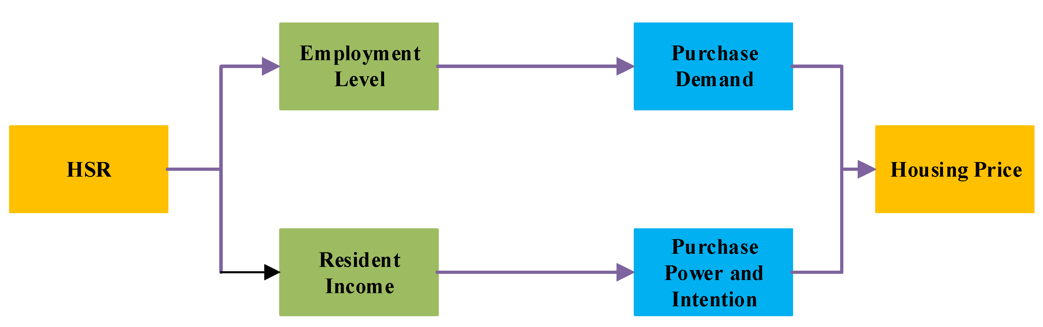
2.1. Direct and Indirect Impact of HSR on Housing Prices

From the perspective of direct impact, HSR, as part of the transportation infrastructure, had a direct effect on real estate investment in cities along the rail line [15]. The advancement of the urbanization process caused cities to continue to expand into the suburbs. With the construction of HSR, many cities built new urban districts and related supporting infrastructure in the area of the HSR station to guide the city to expand and develop in the region [12]. This policy directly promoted cities’ real estate investment and the development of the real estate industry. Therefore, this paper proposes Hypothesis 1.

Hypothesis 1.

The construction of HSR can boost housing prices in cities along the rail line.

From the perspective of indirect effects, the impact mechanism is shown in Figure 3. On the one hand, the construction of HSR increased regional accessibility between cities [20]. By reducing commuting costs, HSR can expand the scope of labor searches, increase labor force participation in cities along the railway, and attract relevant people to these cities [7]. At the same time, HSR cities gradually improved the urban living environment and infrastructure around the new district, and improved the level of urban construction. In this way, HSR can entice labor to migrate from relatively underdeveloped areas to HSR cities [25]. The inflow and increase of labor had a major impact on urban real estate prices. Research by Määttänen and Terviö [26] suggested that labor inflows contributed to rising urban real estate prices. In the context of accelerating urbanization, housing is the most basic requirement when labor flows into cities, and it is large-scale [27]. Therefore, the increase in the employment population brought about by the construction of HSR also promoted the development of the real estate market. On the other hand, the construction of HSR enhanced economic ties between cities in different regions, which spread the economies of large cities to areas with relatively backward economies [22]. This led to rapid economic development in these backward areas, significantly increasing the income level of residents along the rail line. Real estate economists believe that housing is a normal commodity and that buyers allocate housing resources through market price competition. When the disposable income of residents generally increases, households without housing will be willing to pay higher prices in order to obtain housing, and the increase in income will also stimulate households with existing housing to purchase multiple housing properties [26]. Consequently, the price of commercial housing in the market is pushed up from the demand side [28]. Therefore, this study proposes Hypotheses 2 and 3.

Hypothesis 2.

The construction of HSR can promote the increase in housing prices along the rail line by increasing the employment level of cities.

Hypothesis 3.

The construction of HSR can increase the income level of urban residents and, thus, promote the rise in housing prices.

2.2. City Size Heterogeneity Analysis

Due to the heterogeneity of city size, the difference in urban living costs is also great [29]. Compared with the small and medium-sized cities that are located along the rail line, enterprises that opened in large cities need to bear high daily operating expenses. As long as the marginal transportation cost of the company is lower than the marginal benefit brought by the savings in operating expenses when moving out of a large city, the company has an incentive to move to a medium or small-sized city along the rail line [11]. Along with the flow of these enterprises to small and medium-sized cities along the rail line, the economic and labor environments will be improved for enterprises that move inland. The construction of HSR enhanced economic ties between different regions, making the economies of large cities spread to smaller, relatively backward areas along the rail line [29]. It also reduced the commuting costs [25], and made it easier for population and resources to move from large cities to small and medium-sized cities. This drove the development of these small and medium-sized cities and promoted the rapid rise of housing prices in these areas. However, for large cities with more developed economies and higher housing prices, the impact of HSR operation on housing prices may not be significant [15]. Therefore, this paper proposes Hypothesis 4.

Hypothesis 4.

The impact of HSR on housing prices will show obvious differences at the urban scale, and the construction of HSR in small and medium-sized cities will have a greater impact on housing prices than in large cities.

2.3. Regional Heterogeneity Analysis

Although the development of HSR can improve the accessibility of the country, the marginal benefits of cities in different regions are different. The research of Huang et al. [30] showed that HSR results in a big difference in housing prices in different regions. The economy and urban density in the eastern, central, and western regions vary greatly [31], and the level of economic development and housing prices in different regions are also far apart [4]. The accessibility, the level of urban economy, and the degree of regional economic integration of the eastern region are significantly ahead of those in the central and western regions [5] Therefore, the convenience brought by the operation of HSR had a lesser, marginal impact on the eastern region’s economy but had a greater impact on the central and western regions. The level of economic development had a significant impact on housing prices [32]. Thus, we can say that the impact of HSR operation on housing prices should also show obvious regional differences. Based on the above reasons, we propose Hypothesis 5.

Hypothesis 5.

The impact of HSR on housing prices will show significant regional differences, with a higher impact on the central and western regions than on the eastern regions.

3. Methodology and Data

3.1. Data Model

The main purpose of this paper is to scientifically evaluate the total impact of HSR on housing prices. As time changes, the changes in housing prices mainly come from two sources. Part of the effect is the “time effect” formed by natural changes in growth, economic situation over time, fiscal policy, etc. The other part is the “policy-treated effect” caused by the HSR. The key to the problem is how to distinguish the “time effect” from the “policy-treated effect” of HSR construction. Therefore, this paper used the difference-in-difference (DID) model to solve this problem [22]. The difference-in-difference (DID) model can be used to evaluate the effect of a policy, effectively separating the “time effect” from “policy-treated effect”, and it is robust [33]. It can separate the net effect of HSR, i.e., with the “HSR cities” as the treated group and the “non-HSR cities” as the control group. It is assumed that the housing prices of the treated group and the control group have the same “time effect” trend before the operation of HSR, and the difference between the two groups after the HSR operation is caused by the “HSR operation effect”. The DID model to study the influence of HSR on housing prices is shown in Equation (1).

$$Y_{it}={\alpha }_0+{\alpha }_{1}cit{y}_{it}\times yea{r}_{it}+{\mu }_i+{\epsilon }_{it},$$

(1)

where Y_it refers to the average selling price of commercial houses of city i in period t; city_it = 1 represents HSR cities; otherwise, city_it = 0; year_it = 0 represents preconstruction; otherwise year_it = 1; α₁ indicates the impact of HSR on housing prices, μ_i is the individual fixation effect, and ε_it is residual.

In fact, the heterogeneity between cities is very large, and it is difficult to meet the common trend hypothesis. Therefore, it is better to select a batch of “non-HSR cities” whose characteristics are “as similar as possible” to the treated group as the control group before DID processing. The propensity score matching (PSM) developed by econometric economists such as Heckman [34], and Rosenbaum and Rubin [35] can eliminate sample selection bias. Consistent with Baier et al. [36], this paper establishes a Logit regression model to calculate the propensity scores. The dependent variable in the model is a binary dummy variable, where city_it = 1 denotes the treated group, and city_it = 0 denotes the control group. The independent variable is a number of indicators for evaluating the similarity between the two groups. Thus, we can calculate the probability that each city becomes an HSR city, i.e., the propensity score.

$$P_i(X)=\mathrm{Pr}(cit{y}_{it}=1|X_{it})=F[h(X_{it})],$$

(2)

where city_it is a virtual variable; when a city has HSR, city_it = 1; otherwise, city_it = 0; X_it represents the characteristic variables of city i that affect the probability of the city becoming an HSR city, h (·) is a linear function, and F (·) is a logistic function. According to the calculated propensity score, the “non-HSR cities” that match the HSR cities are selected. The matching criterion is that the trend score must achieve balance. On the one hand, this balance means that the score of the treated group city is as similar as possible to the scores of the corresponding control city. On the other hand, there is no significant difference between the treated group and the control group.

PSM can solve the problem of sample selection bias, but it is unable to avoid the endogeneity problem caused by missing variables. DID can solve the endogeneity problem and get the “policy-treated effect”, but it is unable to solve the sample deviation problem. Therefore, this study constructed a PSM-DID model to accurately estimate the effect of HSR on housing prices. The PSM-DID model is shown in Equation (3).

$$Y_{it}={\alpha }_0+{\alpha }_{1}cit{y}_{it}\times yea{r}_{it}+{\beta }_1{X}_{it}+{\mu }_i+{\epsilon }_{it},$$

(3)

where X_it is a series of control variables that affect the changes of housing prices. These control variables not only affect the city’s housing prices, but also affect whether the city can become an HSR city. Other variables are the same as in Equation (1). Equation (3) is the baseline model for evaluating the effect of HSR.

3.2. Variable Description

This study chose the time dummy variable (year_it), as well as the urban virtual variable (city_it) and its interaction term ($cit{y}_{it}\times yea{r}_{it}$), as explanatory variables. We also used the average selling price of commercial houses (HOUPR) [37] in each city as an indicator to reflect the city’s housing prices. Based on existing research, this paper selected the following control variables:

(1)

The economic growth level is measured by gross domestic product (GDP) per capita. The GDP per capita reflects the level of urban economic development. Mayer’s [38] review study also pointed out that GDP is an important factor affecting housing prices. The higher the city’s GDP is, the more developed the city’s economy is, which promotes the increase in real estate prices [29]. Therefore, the impact of economic growth level on housing prices is expected to be positive.

(2)

Population level is measured by the total population at year-end. The urban population level reflects the impact of city scale on housing prices. On the one hand, a higher level of population means a larger market. The increase in population leads to a “centripetal force effect” and an increase in housing demand [37], thereby raising housing prices. On the other hand, the operation of HSR can increase city accessibility and reduce commuting costs between cities. It can lead to the flow of people or factors from large cities with a higher population level to small and medium-sized cities [39]. Therefore, the impact of population level on housing prices is expected to be positive.

(3)

Education level is measured by collections of public libraries per 100 persons. As people pay more and more attention to education, the level of urban education becomes an important factor affecting residents’ choices of housing. In China, parents attach great importance to the education of their children, and it is very common to compete for school district houses. Therefore, the coefficient of education level is expected to be positive [40].

(4)

Medical level is measured by the number of beds in hospitals and health centers. As people pay more attention to health, the level of urban medical care plays an increasingly important role in peoples’ choice of location. The medical level is an important indicator of the level of public services in the region and an important factor in attracting population. Good medical standards became an important factor in raising housing prices.

(5)

Investment in fixed assets is measured by total investment in fixed assets. Investment not only causes the accumulation of material but also has a certain impact on housing prices [41]. On the one hand, the increase in fixed-asset investment may lead to an increase in supply, thereby reducing housing prices. On the other hand, an increase in fixed-asset investment may lead to the agglomeration of labor, resulting in an increase in demand, thereby raising housing prices. Therefore, the direction of the impact of investment in fixed assets on housing prices is uncertain.

3.3. Determination of HSR Operation Time Point and Sample Selection

3.3.1. Determination of HSR Operation Time Point

Consistent with Shaw et al. [6], this article selected 2012 as the time point for the HSR operation. The period of 2008–2011 was defined as the time before the operation of the HSR, while 2012–2016 was defined as the period after the operation of the HSR. It would be unreasonable to use all the remaining HSR cities before 2012 as a control group because many cities gradually constructed HSR every year after 2012. As a result, this study removed the HSR cities after 2012 from the control group.

3.3.2. Sample Selection

This paper selected 285 prefecture-level cities in China from 2008–2016 as our research sample. Cities with less data were supplemented by querying relevant city websites, and cities with missing data were deleted. In the end, we obtained 148 cities and 1332 city–year observations from 2008 to 2016. The relevant HSR data were collected according to the “Medium- and Long-Term Railway Network Plan (2008)”, the train timetable, and the HSR network. Other data were from the Divisions of Administrative Areas of Cities, the Wind Database, and China Real Estate Information. Because HSRs are built on the outskirts of cities, they are far from the city center. Therefore, this paper used total city data instead of city district data. To suppress possible heteroscedasticity, the regression coefficient can accurately express the elastic relationship between variables. This study dealt with some variables with a logarithmic treatment, and the percentile variables were not processed [22]. The definitions and descriptions of the variables are shown in

Table 1. Definitions and descriptive statistics of variables. HSR—high-speed rail; GDP—gross domestic product.

Variable	Definition	Mean	SD	Minimum	Maximum
HOUPR	The average sales price of commercial housing	4847.139	3894.481	901	45,146.500
CITY	Whether or not HSR services exist (yes = 1 and no = 0)	0.365	0.482	0	1
GDP	GDP per capita	43,202.240	32,974.840	3602	256,877
PEO	Total population at year-end	422.953	283.620	16.520	1446
EDU	Collections of public libraries per 100 persons	82.006	120.627	2.300	2187.390
MED	Number of beds of hospitals and health centers	15,848.070	16,141.380	1279	126,838
INVEST	Total investment in fixed assets	1492.436	3867.747	17.125	130,143

.

All samples in this paper were divided into the treated group and the control group. Cities with HSR before 2012 were classified into the treated group, with a total amount of 54 cities. Cities without HSR before and after 2012 were classified into the control group. In addition, in order to compare the heterogeneity of city scale, this paper also further divided full samples into large cities and small and medium-sized cities. In order to compare regional heterogeneity, this paper divided the full sample into eastern cities and central and western cities.

4. Empirical Analysis

4.1. The Effect of HSR on Housing Prices

Table 2. Baseline regression results.

Variable	lnHOUPR
	(1)	(2)	(3)	(4)	(5)	(6)
$Cit{y}_{it}\times Yea{r}_{it}$	0.1186 *** (0.0579)	0.1137 *** (0.0506)	0.1240 *** (0.0481)	0.1688 *** (0.0466)	0.1465 *** (0.0434)	0.1511 *** (0.0434)
lnGDP		0.3055 *** (0.0225)	0.3183 *** (0.0222)	0.2674 *** (0.0231)	0.2342 *** (0.0200)	0.2145 *** (0.0219)
lnPEO			0.1558 *** (0.0129)	0.1679 *** (0.0129)	0.0431 *** (0.0163)	0. 0272 * (0.0175)
lnEDU				0.1170 *** (0.0186)	0.0842 *** (0.0174)	0.0775 * (0.0169)
lnMED					0.1951 *** (0.0177)	0.1750 *** (0.0187)
lnINVEST						0.0484 *** (0.0173)
Observation	1332	1332	1332	1332	1332	1332
Adjusted R2	0.3627	0.5000	0.5490	0.5678	0.6059	0.6076

Robust standard errors are in parentheses. *** represents significance at the 1% level; ** represents significance at the 5% level; * represents significance at the 10% level.

shows the regression results of HSR on housing prices. Model 1 only analyzed the impact of HSR on housing prices, without adding control variables. As shown in model 1, the coefficient of the $cit{y}_{it}\times yea{r}_{it}$ variable is significantly positive at the 1% level. This indicates that, compared with non-HSR cities, HSR can significantly increase the housing prices of cities along the rail line. Therefore, Hypothesis 1 was initially verified. Secondly, in order to verify the robustness of Hypothesis 1, models 2–7 added control variables. This paper found that the coefficients of HSR were still statistically significantly positive at the level of 1%. The results indicate that the construction of HSR significantly promoted the rise of housing prices along the rail line. In the case of added control variables, Hypothesis 1 was still robust. At the same time, after the addition of control variables, the impact coefficient of HSR on real estate prices along the rail line decreased. This suggests that, if the relevant factors are not controlled, the impact of HSR on urban housing prices may be overestimated.

As shown in Table 2, the GDP per capita coefficient was significantly positive at the level of 1%. The study of Krakstad and Oust [42] proved that the impact of GDP on housing prices is weakly exogenous based on Norwegian data. However, most scholars [43] studied China’s data and found that GDP has a significant positive impact on housing prices. Similar to Yingchao et al. [37], we find that, on average, a GDP per capita increase of 1% increased housing prices by 0.21%. This result shows that the level of economic development in the region can significantly affect housing prices. The faster the local economy develops, the higher the housing prices rise. The coefficient of lnPEO was still significant after adding various control variables. This shows that the increase in population will increase housing demand to a certain extent, thereby raising housing prices, which is also in agreement with most research conclusions [27]. The influence coefficients of education level and medical level on housing prices were also significantly positive. This implies that the improvement of the level of urban infrastructure affected the housing prices of cities to some extent. The coefficient of urban fixed-asset investment was also significantly positive. This shows that the positive effect of fixed-asset investment brought about by the construction of HSR on housing prices is higher than the negative effect. Overall, all estimates indicated that HSR has a significantly positive impact on housing prices, regardless of whether or not control variables are added.

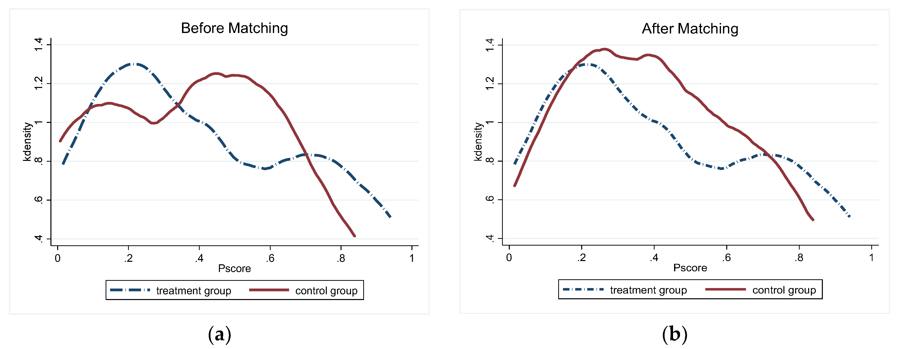
4.2. Test Based on the PSM-DID Model

To overcome the systematic difference between the trend of HSR cities and non-HSR cities and to reduce the selection bias of the DID method, this paper used the PSM-DID method to conduct the robustness test. Firstly, for specific estimation, this paper used the kernel method proposed by Heckman et al. [44] to calculate the propensity score. Referring specifically to Abadie et al. [45], the estimated function is as follows:

$$g(p_i,p_j)=\frac{K(\frac{p_i-p_j}{h})}{{\displaystyle \sum _{j\in (T=0)}K(\frac{p_i-p_j}{h})}},$$

(4)

where p_i is the probability of constructing HSR in the treated group cities, p_j is the probability of constructing HSR in the control group cities, h is the specified bandwidth, and function g (p_i, p_j) is the weight applied when the non-HSR city is used as the control group. Then, we plotted the kernel density function curve as shown in Figure 4. According to Figure 4a, before the kernel matching, the probability density distributions of the two groups were significantly different. This may cause serious estimates of bias without PSM. After matching, it can be seen from Figure 4b that the probability density distributions of the two remaining samples tended to be consistent. This indicates that the characteristics of all aspects of the sample cities after matching were very close, and the sample selection bias was basically eliminated.

In addition, before performing PSM-DID estimation, it is also necessary to test the common support hypothesis, that is, whether the mean values of the covariates of the experimental group and the control group are significantly different after matching. If there is no significant difference, the PSM-DID method is supported [46].

Table 3. Difference-in-difference based on propensity score matching (PSM-DID) common support hypothesis.

Variable	Mean Control	Mean Treated	Diff	|t|	P > |t|
lnHOUPR	8.023	8.316	0.293	4.49	0.0003 ***
lnGDP	10.375	10.340	−0.035	0.43	0.5727
lnPEO	5.590	5.527	−0.063	0.74	0.8703
lnEDU	4.152	4.148	−0.003	0.06	0.8029
lnMED	9.177	9.142	−0.035	0.43	0.6726
lnINVEST	6.500	6.483	−0.016	0.22	0.8265

*** represents significance at the 1% level; ** represents significance at the 5% level; * represents significance at the 10% level.

presents the results of the common support hypothesis. The test results showed an insignificant difference among all control variables after matching, which indicates that the PSM-DID method is reasonable.

The results in

Table 4. HSR and housing prices: PSM-DID robustness test.

Outcome Var.	lnHOUPR	Standard Error	|t|	P > |t|
Before
Control Treated	8.023 8.316
Diff (T−C)	0.293	0.061	4.82	0.000 ***
After
Control	8.201
Treated	8.729
Diff (T−C)	0.528	0.059	8.95	0.000 ***
Diff-in-Diff	0.235	0.085	2.78	0.006 ***

*** represents significance at the 1% level; ** represents significance at the 5% level; * represents significance at the 10% level.

show that, after using the PSM-DID method, the effect coefficient of lnHOUPR was 0.235, and it was significant at the 1% level. Therefore, HSR still significantly increases housing prices. The results of the PSM-DID estimation were not significantly different from the previous DID results. The PSM-DID results further supported the empirical conclusions above. The effect of HSR on housing prices was significantly positive.

4.3. City Size Heterogeneity Analysis

The results of the above analyses showed that the operation of HSR can significantly increase city housing prices. Does the lifting effect differ for cities of different scales? According to the Notice on Adjusting the Standard of City Size Division [47] issued by the China State Council and the urban population at the end of 2016, the whole sample was divided into two subsamples of large cities and small and medium-sized cities. According to the city population at the end of 2016, the PSM-DID regression was performed on the subsamples to explore the differences in the impact of HSR on housing prices in cities of different scales. The regression results are shown in

Table 5. Regression results of city size heterogeneity analysis.

	lnHOUPR
	Large Cities	Small and Medium-Sized Cities
$Cit{y}_{it}\times Yea{r}_{it}$	0.133	0.120
Standard Error	0.166	0.036
|t|	0.800	3.320
P > |t|	0.427	0.001 ***
Adjusted R2	0.408	0.337

*** represents significance at the 1% level; ** represents significance at the 5% level; * represents significance at the 10% level.

. Similar to the results of Haynes [15], we also found significant differences in the effects of HSR on housing prices at different scales. In large cities, the coefficient of $cit{y}_{it}\times yea{r}_{it}$ was positive but not statistically significant, while the coefficient of $cit{y}_{it}\times yea{r}_{it}$ in the small and medium-sized cities was positive and significant at the level of 1%. This shows that the positive effect of HSR on the increase in housing prices is stronger in small and medium-sized cities. Hypothesis 4 is, therefore, verified. On the one hand, for small and medium-sized cities, the population is small. The operation of HSR increased the mobility of residents and increased the willingness of residents to purchase property, thus significantly increasing housing prices. For large cities, the population and housing demand are large, and housing prices were originally higher. Therefore, the marginal effect of HSR was small. On the other hand, the operation of HSR can reduce commuting costs, which may cause a population flow out of large cities with greater density to small and medium-sized cities with lower density. It can also lead to an increase in housing demand in small and medium-sized cities. Finally, in terms of the effect of HSR investment, large-scale investment in HSR construction can drive the economic development of small and medium-sized cities and, thus, increase their housing prices. For large cities with high economic levels, the marginal effect of HSR investment on housing prices is nonsignificant. Although, we can say that HSR increases housing prices, the impact is affected by the size of the city. The significant positive effect of the full sample may be driven by small and medium-sized cities.

4.4. Regional Heterogeneity Analysis

This paper divided the full sample into eastern cities and central and western cities according to the China Urban Area Division Standard promulgated [48] by the National Bureau of Statistics.

Table 6. Regression results of regional heterogeneity analysis.

	lnHOUPR
	Eastern Region	Central and Western Regions
Diff-in-Diff	0.079	0.183
Standard Error	0.051	0.058
|t|	1.56	3.16
P > |t|	0.120	0.002 ***
Adjusted R2	0.241	0.296

*** represents significance at the 1% level; ** represents significance at the 5% level; * represents significance at the 10% level.

shows that the impact of HSR on housing prices in eastern cities is not obvious. However, the effect coefficient of HSR operation on housing prices in central and western cities was 0.183 and was significant at the 1% level. On the one hand, the economic level, integration level, and regional accessibility between cities in the eastern region were already high before the operation of HSR, which limited the marginal impact of the operation of HSR in the region. Therefore, the effect on housing prices in the eastern region by the operation of HSR was not significant. For the central and western regions, the accessibility between regions was low before the construction of the HSR, and the HSR significantly improved regional accessibility and attracted the external population. On the other hand, housing prices in the eastern cities were higher, and local governments tightened the intensity of housing prices; thus, there was less room for housing prices to increase in the eastern cities. For the central and western cities, the urban economic level and housing price base were low before the construction of the HSR. Therefore, the marginal effect of the HSR construction was strong. In general, central and western regions cities played an important role in the total effect of HSR.

5. Mechanism Test

From the empirical results, it can be seen that HSR can significantly increase housing prices along the rail lines; however, what is the mechanism of HSR that causes housing prices to increase? As explained in the theoretical analysis of the second section, the construction of HSR improves the regional accessibility between cities, and the labor force can find better jobs by increasing commuting cost [46]. With the construction of HSR, the income level of residents within the vicinity of the HSR area also improves. This income level increase increases the purchase demand of residents and increases the purchasing power and willingness to purchase, thereby increasing the cities’ housing prices. This study used Baron and Kenny’s [49] method to verify the existence of employment and resident income mechanisms.

Firstly, to verify the existence of the employment mechanism, we used a regression of the $cit{y}_{it}\times yea{r}_{it}$ and housing prices. If the $cit{y}_{it}\times yea{r}_{it}$ coefficient is significant, this indicates that the HSR increased urban housing prices. Secondly, we used a regression of the $cit{y}_{it}\times yea{r}_{it}$ and employment level. If the $cit{y}_{it}\times yea{r}_{it}$ coefficient is significant, this indicates that the HSR improved the urban employment level. Thirdly, we input the $cit{y}_{it}\times yea{r}_{it},$ housing prices, and employment level variables into the model at the same time for regression. If the coefficient of the $cit{y}_{it}\times yea{r}_{it}$ is not significant, or if it is significant but the coefficient is reduced, this proves that the construction of the HSR increased housing prices by increasing the urban employment level. The model is shown below.

To verify the impact of HSR construction on housing prices,

$$Y_{it}={\alpha }_0+{\alpha }_{1}cit{y}_{it}\times yea{r}_{it}+{\alpha }_2{X}_{it}+{\mu }_i+{\epsilon }_{it}.$$

(5)

To verify the impact of HSR construction on the employment level,

$$E_{it}={\beta }_0+{\beta }_{1}cit{y}_{it}\times yea{r}_{it}+{\beta }_2{X}_{it}+{\mu }_i+{\epsilon }_{it}.$$

(6)

Putting the $cit{y}_{it}\times yea{r}_{it}$ and employment level into the equation at the same time,

$$Y_{it}={\gamma }_0+{\gamma }_{1}cit{y}_{it}\times yea{r}_{it}+{\gamma }_2{E}_{it}+{\gamma }_3{X}_{it}+{\mu }_i+{\epsilon }_{it}.$$

(7)

Here, E_it is the employment level variable, expressed by the number of employed people at year-end. To reduce the heteroscedasticity and sample dispersion, this study used logarithmic processing. We used the weighted least squares method to correct the heteroscedasticity and then performed the White test. The test results show that the p-values in the regression analysis all exceeded 0.05, indicating that the heteroscedastic problem was solved [50]. From the results of

Table 7. Intermediary mechanism test—employment level.

Variable	lnHOUPR	lnEM	lnHOUPR
$Cit{y}_{it}\times Yea{r}_{it}$	0.1187 *** (0.0579)	0.0795 *** (0.0385)	0.0303 (0.0372)
lnEM			0.1101 *** (0.0647)
Observation	1332	1332	1332
Adjusted R2	0.3627	0.3618	0.7136

Robust standard errors are in parentheses. *** represents significance at the 1% level; ** represents significance at the 5% level; * represents significance at the 10% level.

, we can see that the first regression results showed that the construction of HSR significantly increased urban housing prices. The results of the second step of the regression showed that the regression coefficient between HSR construction and employment level was significantly positive, indicating that the construction of HSR promoted the improvement of urban employment. The third-step regression results showed that the housing price coefficient was no longer significant. This result indicates that HSR improved urban housing prices by increasing urban employment levels. Hypothesis 2 is, therefore, verified.

Then, to verify the resident income level, we used (1) a regression of the $cit{y}_{it}\times yea{r}_{it}$ and housing prices. If the $cit{y}_{it}\times yea{r}_{it}$ coefficient is significant, this indicates that the HSR increased urban housing prices; (2) a regression of the $cit{y}_{it}\times yea{r}_{it}$ and resident income level. If the $cit{y}_{it}\times yea{r}_{it}$ coefficient is significant, this indicates that the HSR improved the resident income level; (3) a regression of the $cit{y}_{it}\times yea{r}_{it}$, housing prices, and resident income level at the same time. If the coefficient of $cit{y}_{it}\times yea{r}_{it}$ is not significant, or if it is significant but the coefficient is reduced, this proves that the construction of the HSR increased housing prices by increasing resident income level. The model is shown below.

To verify the impact of HSR construction on housing prices,

$$Y_{it}={\alpha }_0+{\alpha }_{1}cit{y}_{it}\times yea{r}_{it}+{\alpha }_2{X}_{it}+{\mu }_i+{\epsilon }_{it}.$$

(8)

To verify the impact of HSR construction on resident income level,

$$S_{it}={\eta }_0+{\eta }_{1}cit{y}_{it}\times yea{r}_{it}+{\eta }_2{X}_{it}+{\mu }_i+{\epsilon }_{it}.$$

(9)

Putting the $cit{y}_{it}\times yea{r}_{it}$ and resident income level into the equation at the same time,

$$Y_{it}={\lambda }_0+{\lambda }_{1}cit{y}_{it}\times yea{r}_{it}+{\lambda }_2{S}_{it}+{\lambda }_3{X}_{it}+{\mu }_i+{\epsilon }_{it}.$$

(10)

Here, S_it is the resident income level variable. This paper used the resident savings deposit as the measure of the resident income level. To reduce heteroscedasticity and sample dispersion, this study used logarithmic processing, and the White test results were robust. From the results in

Table 8. Intermediary mechanism test—resident income.

Variable	lnHOUPR	lnSAV	lnHOUPR
$Cit{y}_{it}\times Yea{r}_{it}$	0.1187 *** (0.0579)	0.1543 *** (0.0752)	0.0289 (0.0362)
lnSAV			0.5813 *** (0.0327)
Observation	1332	1332	1332
Adjusted R2	0.3627	0.3658	0.7264

Robust standard errors are in parentheses. *** represents significance at the 1% level; ** represents significance at the 5% level; * represents significance at the 10% level.

, we can see that the first regression results showed that the construction of HSR significantly increased housing prices. The results of the second step of the regression showed that the regression coefficient of $cit{y}_{it}\times yea{r}_{it}$ was significantly positive, indicating that the construction of HSR promoted the improvement of resident income level. The third-step regression results showed that the $cit{y}_{it}\times yea{r}_{it}$ coefficient was no longer significant. This indicates that HSR improved urban housing prices by increasing resident income level. In other words, resident income level plays an important role in the impact of HSR on housing prices. Hypothesis 3 is, therefore, verified. So far, the two mechanisms of this paper were verified.

6. Robustness Test

6.1. Change Time Window Test

The empirical analysis of this paper showed that the construction of HSR significantly expanded the housing price gap between “HSR cities” and “non-HSR cities”. However, the above empirical test used urban data from 2008 to 2016. The results reflected the average impact of the operation of the HSR (2012–2016) relative to before the construction of the HSR (2008–2011). The test did not reflect the magnitude and difference of this effect in different time periods before and after the construction of HSR. The difference in different time windows may be very large. Therefore, it is very necessary to observe the effect of different time windows before and after the HSR operation point. To identify whether the effect of HSR on housing prices changed with the length of the sample, this study identified the sensitivity of the policy to time changes by changing the regression time interval. This paper selected samples of before and after one year, two years, and three years. If there are no significant changes in regression coefficient and significance, this indicates that the estimation results are robust. The results are shown in

Table 9. Change time window width test.

	lnHOUPR
	One Year	Two Years	Three Years	Four Years
$Cit{y}_{it}\times Yea{r}_{it}$	0.0741 *	0.0721 *	0.1046 ***	0.1510 ***
Standard Error	0.0687	0.0606	0.0495	0.0434
|t|	1.0800	1.1900	2.1100	3.4800
P > |t|	0.2820	0.2350	0.0350	0.0010
Adjusted R2	0.5869	0.5334	0.5750	0.6076

*** represents significance at the 1% level; ** represents significance at the 5% level; * represents significance at the 10% level.

. In the four regressions, the coefficients of the construction of HSR were statistically insignificant. This still supports the previous conclusions. Therefore, we can confidently conclude that the impact of HSR construction on housing prices is significantly positive.

6.2. Placebo Test

To reduce the impact of unobserved factors on the results of the empirical analysis, this paper used a counterfactual method [51] for placebo testing. This study artificially set the HSR operation time points to test the effect of HSR on housing prices by using the data from the years 2008 to 2012. The 2009, 2010, and 2011 years were taken as hypothetical HSR operation time points to test the impact of HSR on housing prices. If the coefficient is insignificant, this indicates that the increase in urban housing prices is caused by the construction of the HSR, rather than other unobserved factors. Otherwise, the regression results are not robust. The results of the placebo test are shown in

Table 10. Placebo test results.

Variable	lnHOUPR
	2009		2010		2011
$Cit{y}_{it}\times Yea{r}_{it}$	0.0148 (0.0917)	0.0266 (0.0633)	0.0057 (0.0767)	0.0251 (0.0559)	−0.0147 (0.0765)	0.0061 (0.0572)
lnGDP		0.1888 *** (0.0258)		0.1784 *** (0.0256)		0.1949 *** (0.0274)
lnPEO		−0.0464 ** (0.0263)		−0.0078 (0.0206)		0.0303 * (0.0208)
lnEDU		0.0544 *** (0.0227)		0.0702 *** (0.0220)		0.0754 *** (0.0228)
lnMED		0.2277 *** (0.0253)		0.2142 *** (0.0230)		0.1849 *** (0.0231)
lnINVEST		0.0761 *** (0.0220)		0.0520 *** (0.0203)		0.0590 *** (0.0536)
Observation	740		740		740
Adjusted R2	0.2922	0.5644	0.3416	0.5823	0.2974	0.5564

Robust standard errors are in parentheses. *** represents significance at the 1% level; ** represents significance at the 5% level; *represents significance at the 10% level.

. The results showed that the HSR effect became statistically insignificant after we artificially set the HSR operation time points. Regardless of whether 2009, 2010, or 2011 was selected as the hypothetical HSR construction time point, there was no significant change in the housing price difference between the treated group and the control group. In other words, we can conclude that the above conclusions are not the result of a placebo effect over time. The operation of the HSR has a significantly positive impact on housing prices.

In summary, based on the results of the above robustness tests, we have reason to believe that the estimation results and conclusions of this paper are very stable. Therefore, we can conclude that the HSR indeed promoted the rise in housing prices along the rail lines.

7. Conclusions

The rapid development of the HSR network resulted in revolutionary changes to China’s transportation infrastructure. HSR increased the accessibility between cities, and promoted the flow of various factors such as population and capital. Moreover, its large-scale investment also promoted the level of investment in cities and, thus, promoted the growth of urban economy. Therefore, it brought about changes in the real estate industry. This paper used data from 2008 to 2016 in China’s prefecture-level cities to construct a PSM-DID model to analyze the impact of HSR on housing prices along the rail line, as well as HSR’s associated impact mechanisms. This study also subdivided cities of different sizes into large cities and small and medium-sized cities to study the differences in the impact of HSR on cities of different scales. Considering the different levels of economic development in different regions of China, this study also subdivided cities into eastern cities and central and western cities. The major conclusions of this paper are described below.

Firstly, HSR significantly promoted the rise of housing prices in HSR cities along the rail line, especially in the “central and western cities” and “small and medium-sized cities”. It widened the housing price gap between HSR cities and non-HSR cities, but had an insignificant effect on housing prices in eastern cities and large cities. Because the “space–time compression” effect of HSR inevitably led to an increase in city’s accessibility, it brought about better living conditions and lower transportation costs in the surrounding areas, which led to an increase in housing demand, and eventually led to an increase in housing prices. However, the population in cities with higher living costs may be transferred to other cities with a lower cost of living along the rail line due to HSR, thus increasing the housing demand of “small and medium-sized cities” and “central and western cities”. Therefore, HSR had a significant effect on housing prices in “central and western cities” and “small and medium-sized cities”, but had an insignificant impact on housing prices in eastern cities and large cities. Secondly, through mechanism analysis, this study found that the construction of HSR increased urban housing prices by affecting employment level and resident income level. The construction of HSR enabled residents to work and live in different cities. This expanded the scope of labor searches, raised the level of economic development of HSR cities, and raised the income level of residents. As a result, the development of the real estate industry in the HSR cities was facilitated, and the cities’ housing prices were raised.

Stabilizing housing prices is an important way to make the economy develop steadily. On the one hand, large-scale investment in HSR drove the improvement of urban fixed-asset investment and other investment levels. On the other hand, the development of HSR enhanced the accessibility between cities, reduced the commuting costs of residents, and improved the convenience of transportation. Our research results showed that the HSR network led to the concentration of resources and population from non-HSR cities to HSR cities. Furthermore, HSR can also spread the population and resources from cities with high living costs to the small and medium-sized cities in the central and western regions along the rail line. Based on the perspective of housing prices, this paper studied the differences in the impact of HSR construction on HSR cities and non-HSR cities. The results provided positive evidence for local governments to formulate policies for stabilizing housing prices according to local conditions. When the government formulates housing prices control policies, the effects of HSR should be considered comprehensively. Local governments should constantly improve relevant policies, introduce measures, and stabilize housing prices. In particular, they should pay attention to regulating fluctuations in housing prices in small and medium-sized cities in the central and western regions under the influence of HSR. This paper used PSM-DID method to analyze the impact of HSR on housing prices, and made some contributions to HSR research, but there were still some limitations: (1) the impact of HSR on housing prices at different time points was not distinguished, such as when the HSR investment decision became publicly known, when the construction started, when the HSR opened, etc.; (2) the spatial effect of HSR was not considered. These limitations can be addressed in future research.

References

1. NRA. China’s High-Speed Rail Information. Available online: http://www.nra.gov.cn/xwzx/zlzx/hytj/201904/P020190426367686178375.pdf (accessed on 21 November 2016).
2. NDRC. Mid-to-Long Term Railway Network Plan. Available online: http://www.nra.gov.cn/jgzf/flfg/gfx_wj/zt/other/201607/t20160721_26055.shtml (accessed on 18 December 2018).
3. Wang, S.; Yang, Z.; Liu, H. Impact of urban economic openness on real estate prices: Evidence from thirty-five cities in China. China Econ. Rev. 2011, 22, 42–54. [Google Scholar] [CrossRef]
4. Jia, S.; Zhou, C.; Qin, C. No difference in effect of high-speed rail on regional economic growth based on match effect perspective. Transport. Res. Part A Policy Pract. 2017, 106, 144–157. [Google Scholar] [CrossRef]
5. Chen, Z.; Xue, J.; Rose, A.Z.; Haynes, K.E. The impact of high-speed rail investment on economic and environmental change in china: A dynamic CGE analysis. Transport. Res. Part A Policy Pract. 2016, 92, 232–245. [Google Scholar] [CrossRef]
6. Shaw, S.L.; Fang, Z.; Lu, S. Impacts of high speed rail on railroad network regional accessibility in China. J. Transp. Geogr. 2014, 40, 112–122. [Google Scholar] [CrossRef]
7. Vickerman, R. High-speed rail and regional development: The case of intermediate stations. J. Transp. Geogr. 2015, 42, 157–165. [Google Scholar] [CrossRef]
8. Zheng, S.; Kahn, M.E. China’s bullet trains facilitate market integration and mitigate the cost of mega city growth. Proc. Natl. Acad. Sci. USA 2013, 110, E1248–E1253. [Google Scholar] [CrossRef] [PubMed]
9. Tierney, S. High-speed rail, the knowledge economy and the next growth wave. J. Transp. Geogr. 2012, 22, 285–287. [Google Scholar] [CrossRef]
10. Dong, Y.M.; Zhu, Y.M. Study on the employment effect of the construction of high speed railway—Evidence from 285 cities of China based on PSM-DID method. Econ. Mana. J. 2016, 38, 26–44. [Google Scholar]
11. Willigers, J.; Wee, B.V. High-speed rail and office location choices. J. Transp. Geogr. 2011, 19, 745–754. [Google Scholar] [CrossRef]
12. Hiramatsu, T. Unequal regional impacts of high speed rail on the tourism industry: A simulation analysis of the effects of Kyushu Shinkansen. Transprtation 2016, 45, 1–25. [Google Scholar] [CrossRef]
13. Yun, Z.; Xue-Mei, I. Estimation model of knowledge spillover based on accessibility—Analysis of effect of high speed railway network. Soft. Sci. 2015, 29, 55–58. [Google Scholar]
14. Geng, B.; Bao, H.; Ying, L. A study of the effect of a high-speed rail station on spatial variations in housing price based on the hedonic model. Habitat Int. 2015, 49, 333–339. [Google Scholar] [CrossRef]
15. Chen, Z.; Haynes, K.E. Impact of high speed rail on housing values: An observation from the Beijing–Shanghai line. J. Transp. Geogr. 2015, 43, 91–100. [Google Scholar] [CrossRef]
16. Rosen, S. Hedonic prices and implicit markets: Product differentiation in pure competition. J. Polit. Econ. 1974, 82, 34–55. [Google Scholar] [CrossRef]
17. Minghong, Z.; Qingyuan, Z.; Ruobing, L. A study of the nonlinear and heterogeneity influence of high-speed railway on the real estate prices. Contemp. Financ. Econ. 2017, 9, 3–13. [Google Scholar]
18. Lvhua, W.; Yongxue, L.; Liang, M. Potential Impacts of China 2030 High-Speed Rail Network on Ground Transportation Regional accessibility. Sustainability 2018, 10, 1270. [Google Scholar] [CrossRef]
19. Hou, Q.; Li, S.-M. Transport infrastructure development and changing spatial accessibility in the Greater Pearl River Delta, China, 1990–2020. J. Transp. Geogr. 2011, 19, 1350–1360. [Google Scholar] [CrossRef]
20. Chandra, S.; Vadali, S. Evaluating accessibility impacts of the proposed America 2050 high-speed rail corridor for the Appalachian Region. J. Transp. Geogr. 2014, 37, 28–46. [Google Scholar] [CrossRef]
21. Ke, X.; Chen, H.; Hong, Y. Do China’s high-speed-rail projects promote local economy?—New evidence from a panel data approach. China Econ. Rev. 2017, 44, 203–226. [Google Scholar] [CrossRef]
22. Shao, S.; Tian, Z.; Yang, L. High speed rail and urban service industry agglomeration: Evidence from China’s Yangtze River Delta region. J. Transp. Geogr. 2017, 64, 174–183. [Google Scholar] [CrossRef]
23. Abadie, A. Semiparametric difference-in-differences estimators. Rev. Econ. Stud. 2005, 72, 1–19. [Google Scholar] [CrossRef]
24. Dong, Y.M.; Zhu, Y.M. Can high-speed rail construction reshape the layout of China’s economic space—Based on the perspective of regional heterogeneity of employment, wage and economic Growth. China Indust. Econ. 2016, 10, 92–108. [Google Scholar]
25. Guirao, B.; Campa, J.L.; Casado-Sanz, N. Labour mobility between cities and metropolitan integration: The role of high speed rail commuting in Spain. Cities 2018, 78, 140–154. [Google Scholar] [CrossRef]
26. Määttänen, N.; Terviö, M. Income distribution and housing prices: An assignment model approach. J. Econ. Theory 2014, 151, 381–410. [Google Scholar] [CrossRef] [Green Version]
27. Wang, X.; Hui, E.C.; Sun, J. Population migration, urbanization and housing prices: Evidence from the cities in China. Habitat Int. 2017, 66, 49–56. [Google Scholar] [CrossRef]
28. Rubin, Z.; Felsenstein, D. Supply side constraints in the Israeli housing market the impact of state owned land. Land Use Policy 2017, 65, 266–276. [Google Scholar] [CrossRef]
29. Xie, D.; Lin, X. The effect of urban scale, economic growth to urban housing price. Econ. Geogr. 2014, 34, 70–77. [Google Scholar]
30. Huang, X.B.; Liang, Q.P.; Chen, Z.N.; Liu, S. The Study of the Space Effect of Intercity Rail to Housing Price: A Case of Study on Guangzhou-Zhuhai Intercity Railway. Mod. Urban Res. 2015, 6, 26–31. (In Chinese) [Google Scholar]
31. Youn, H. The effects regional characteristics of housing environment in Seoul upon housing prices. J. Korea Real Estate Anal. Assoc. 2013, 19, 235–253. [Google Scholar]
32. Choi, C.; Jung, H. Does an economically active population matter in housing prices? Appl. Econ. Lett. 2017, 24, 1061–1064. [Google Scholar] [CrossRef]
33. Blundell, R.; Dias, M.C. Evaluation methods for non-experimental data. Fiscal. Stud. 2000, 21, 427–468. [Google Scholar] [CrossRef]
34. Heckman, J. The common structure of statistical models of truncation, sample selection and limited dependent variables. Ann. Econ. Soc. Meas. 1976, 5, 475–492. [Google Scholar]
35. Rosenbaum, P.R.; Rubin, D.B. The central role of the propoensity score in observational studies for causal effects. Biometrika 1983, 70, 41–55. [Google Scholar] [CrossRef]
36. Baier, S.L.; Bergstrand, J.H. Estimating the effects of free trade agreements on international trade flows using matching econometrics. J. Int. Econ. 2009, 77, 63–76. [Google Scholar] [CrossRef]
37. Lin, Y.; Ma, Z.; Zhao, K. The impact of population migration on urban housing prices: Evidence from China’s major cities. Sustainability 2018, 10, 3169. [Google Scholar] [CrossRef]
38. Mayer, C.J. Housing bubbles: A survey. Soc. Sci. Elect. Pub. 2011, 3, 559–577. [Google Scholar] [CrossRef]
39. Hall, P. Magic carpets and seamless webs: Opportunities and constraints for highspeed trains in Europe. Built. Environ. 2009, 35, 59–69. [Google Scholar] [CrossRef]
40. Wen, H.; Xiao, Y.; Zhang, L. School district, education quality, and housing price: Evidence from a natural experiment in Hangzhou, China. Cities 2017, 66, 72–80. [Google Scholar] [CrossRef]
41. Han, L.; Ming, L.U. Housing prices and investment: An assessment of China’s inland-favoring land supply policies. J. Asia. Pac. Econ. 2017, 22, 1–16. [Google Scholar] [CrossRef]
42. Krakstad, S.O.; Oust, A. Are house prices in the Norwegian capital too high? Int. J. Hous. Mark. Anal. 2015, 8, 152–168. [Google Scholar] [CrossRef]
43. Li, Z.F.; Zhang, H. Cost-push or demand-pull: What is driving the housing prices in China? Chin. J. Manag. Sci. 2015, 23, 143–150. [Google Scholar]
44. Heckman, J.J.; Ichimura, H.; Todd, P. Matching as an econometric evaluation estimator. Rev. Econ. Stud. 1998, 65, 261–294. [Google Scholar] [CrossRef]
45. Abadie, A.; Imbens, G.W. On the failure of the bootstrap for matching estimators. Econometrica 2008, 76, 1537–1557. [Google Scholar]
46. Zhang, Y.; Peng, Y.; Ma, C.; Bo, S. Can environmental innovation facilitate carbon emissions reduction? Evidence from China. Energy Policy 2017, 100, 18–28. [Google Scholar] [CrossRef]
47. CSC. The Notice on Adjusting the Standard of City Size Division. Available online: http://www.gov.cn/zhe ngce/content/2014–11/20/content_9225.htm (accessed on 19 January 2016).
48. NBS. The China Urban Area Division Standard. Available online: http://www.stats.gov.cn/tjsj/zxfb/201405 /t20140527_558611.html (accessed on 11 February 2016).
49. Baron, R.M.; Kenny, D.A. The Moderator-mediator Variable Distinction in Social Psychological Research: Conceptual, Strategic, and Statistical Considerations. J. Pers. Soc. Psychol. 1986, 51, 1173–1182. [Google Scholar] [CrossRef] [PubMed]
50. Bond, A.S. Some tests of specification for panel data: Monte Carlo evidence and an application to employment equations. Rev. Econ Stud. 1991, 58, 277–297. [Google Scholar]
51. Wu, W.; Liang, Y.; Wu, D. Evaluating the impact of China’s rail network expansions on local accessibility: A market potential approach. Sustainability 2006, 8, 512–613. [Google Scholar] [CrossRef]
Figure 1. China’s high-speed rail (HSR) plan.
Sustainability 11 03681 g001
Figure 2. Trends of housing prices and accumulated mileage of China’s HSR network over the 2007–2017 period.
Sustainability 11 03681 g002
Figure 3. The mediating effect of employment level and resident income.
Sustainability 11 03681 g003
Figure 4. Comparison of kernel density distributions of propensity scores between the treated group and the control group. (a) Plot of propensity score nuclear density before matching. (b) Plot of propensity score nuclear density after matching.
Sustainability 11 03681 g004