1. Introduction
The M&M theory proposed by Modigliani and Miller [
1] shows that a firm’s financial and operational decision are independent in a perfect capital market. However, Hite et al. [
2] point out that the market is always imperfect in real life, so a firm’s financing and operational decisions will interact each other.
For many small-to-medium-sized enterprises (SMEs), including many startup firms, which are facing high business risks, low-value capital assets, the shortage of liquidity, will get caught up in financial constraints which is a common factor affecting business decision-making. In the case of financial constraints, companies often need to use short-term financing to ease the pressure on funds and maintain the normal operation of the company.
At present, most SMEs have no sufficient financing channels as they mainly rely on bank credit financing. However, due to their own instability and the lack of mortgage assets, most banks will refuse to provide credit loans to them or provide loan services only through fixed asset mortgages.
Trade credit is a short-term business financing that the seller provides for the purchase by allowing the buyer to delay payment, that is, according to the real trade background within the supply chain, the retailer can apply for financing from the supplier based on orders via delayed payment. Due to lack of sufficient initial funding to pay for all the purchases, the retailer chooses to pay a portion of the purchase price before the sales season and repay the debt obligation with sales revenue at the end of the sales season. It has become a popular source of short-term financing which can alleviate the shortage of capital for enterprises and allocate the working capital of upstream and downstream to promote the effective operation of the entire supply chain.
In actual business operations, there are often multi-period loans between suppliers and retailers with long-term cooperative relationships, which is also in line with the interests of all parties in the supply chain. In this paper we consider both a single-period and multi-period Stackelberg game between a supplier (she) and a capital-constrained retailer (he) who can choose to get a loan from a bank or supplier. We use dynamic inventory and capital flow to solve the retailer’s financing and ordering strategies to maximize its expected terminal wealth at the end of the planning horizon.
In this paper, we introduce the retailer’s initial inventory into the one-period static financing model, divide the retailer’s initial inventory and capital into different wealth regions, discuss the optimal strategies of different wealth regions, and consider the retailer’s bankruptcy situation. We also extend to the two-period dynamic financing model with dynamic inventory and capital flow, so as to obtain the Stackelberg equilibrium with the optimal strategy matrix of the retailer and the supplier. We compare the performance of the supply chain under single-period and two-period credit from the bank or the supplier respectively through numerical analysis and illustrate that the trade credit and the two-period setting can improve the supply chain’s performance and maximize both retailer’s and supplier’s expected profit.
The rest of the paper is structured as follows:
Section 2 reviews the relevant literature of trade credit and dynamic inventory. In
Section 3, the general model and its assumptions are described in detail.
Section 4 presents the single-period model under bank and supplier financing respectively to obtain the retailer’s optimal contract parameters and the corresponding supplier equilibrium. In
Section 5, we extend the base model to the two-period case with capital flow and dynamic inventory. Numerical analysis is illustrated in
Section 6. We conclude this paper in
Section 7 with some possible future directions.
2. Literature Review
This work is mainly related to the literature on trade credit and dynamic inventory. Cachon [
3] considers a supplier to provide a supply chain contract to a retailer facing a newsvendor problem and analyzes supply chain coordination within different supply chain contracts. Many subsequent supply chain management literatures are based on this model to add different constraints and explore the optimal strategies of the supply chain.
Xu and Birge [
4] first introduced capital constraints in the classical newsvendor model and studied how the firm’s production decisions are affected by financing decisions under financial constraints. Since then, many scholars have begun to study capital-constrained supply chain. Some researches focus on external financing in the supply chain to alleviate financial constraints. Li et al. [
5] study the dynamic coordination model of financially constrained equity financing companies, in which inventory and financial decisions interacted in the presence of stochastic demand and default risk. Dada and Hu [
6] discuss the optimal loan amount of the newsvendor retailer under capital constraints when the bank determined the interest rate to maximize its own profit. Caldentey and Haugh [
7] show that financial markets can be used as a means of arbitrage to reduce retailers’ capital constraints. Babich and Sobel [
8] use IPO to maximize expected discounts to coordinate loan amounts with production and sales. Raghavan et.al [
9] consider the joint financing decision of a retailers and a supplier who are both financial constraints and prove the superiority of joint financing over independent financing. Turcic et al. [
10] explore the merits of reducing the risk of adverse changes in costs in a decentralized supply chain.
Buzacott and Zhang [
11] first began to study the impact of asset-based financing on enterprise inventory management. They demonstrated the importance of joint consideration of production and financing decisions in a start-up setting in which the ability to grow the firm is mainly constrained by its limited capital and dependence on bank financing. On the basis of Buzacott and Zhang’s work, the interfaces of supply chain internal financing under financial constraints have recently attracted substantial interest.
Lai et al. [
12] examine the impact of financial constraint and investigate the supply chain efficiency under preorder mode, consignment mode or the combination of these two modes. They show that with financial constraints, the combination mode is the most efficient mode even if the retailer earns zero internal capital. Zhou and Groenevelt [
13] consider a monopolized bank whose aim is to maximize profits and the manufacturer prefers to choose bank financing. Kouvelis and Zhao [
14] show that supplier financing cannot fully coordinate the supply chain, but can improve the overall performance better than bank financing can. Jing, Chen and Cai [
15] study the retailer’s financial decision under capital constraints with different production cost levels in the case of only bank financing, only trade financing exists and when both financings exist simultaneously.
In recent years, many scholars have begun to expand research on the basis of trade credit. Different from prior research which always focused on trade credit in vertical supply chain relationships, there are some studies of trade credit considering horizontal competition. Peura et al. [
16] illustrate that trade credit can benefit suppliers through horizontal channels. Deng et al. [
17] consider multiple heterogeneous capital-constrained component suppliers and characterize the equilibrium solutions under buyer finance, bank finance and no finance. Lee et al. [
18] study how trade credit responds to various types of competition in supply chains, as well as the impact of trade credit on firm performance.
Capital-constrained supply chain coordination by supply chain contracts provides a novel perspective for trade credit research. Lee and Rhee [
19] show that under inventory financing costs, supply chain contracts including all-unit quantity discount contract, buyback contract, two-part tariff and revenue sharing contract can coordinate the supply chain only when the supplier provide trade credit to the retailer. Kouvelis and Zhao [
20] analyze the use of revenue-sharing contract with working capital coordination for decentralized management of supply chains when there are bankruptcy risks and default costs.
As an integral part of the supply contract, trade credit and inventory management are inextricably linked. Luo, Wei and Shang [
21] show that in the presence of transaction costs, a firm may stock more even if the inventory holding cost increases. Yang et al. [
22] demonstrate how trade credit enhances supply chain efficiency by allowing the retailer to partially share the demand risk with the supplier by transfer stock.
Capital-constrained supply chain under asymmetric information is becoming increasingly widespread vision. Pfohl [
23] analyzes the impact of information cost on the financing strategy of supply chain with constraints of asymmetric information from the perspective of supply chain capital flow optimization. Zheng et al. [
24] investigated an extension of the newsvendor model with demand forecast updating under supply constraints. For the sake of self-interest, in their paper the manufacturer constrains the retailer’s shortening of the lead time by increasing the ordering cost and the limitation of the ordering time and quantity.
There are many other development directions for trade credit research. Chod [
25] proves that trade credit can reduce financial-constrained retailer’s decision deviation from the first-best inventory decision when ordering multiple heterogeneous products. Wang et al. [
26] establish a supplier-led Stackelberg game model by considering supplier’s capital constraint and prove that trade credit can achieve a win-win situation for both sides of the game. Houston et al. [
27] study how retailer bankruptcy affects the bank financing costs of its major suppliers. Tunca et al. [
28] analyze the role and efficiency of buyer inter- mediation in supplier financing.
These studies on trade credit mainly focus on the capital-constrained supply chain in a single sales season, and there are few achievements on supply chain in multi-period situations. In the multi-period situation, the inventory strategy will be transformed from the static inventory to dynamic inventory. Many scholars and teams have made some progress in dynamic inventory. Aggawal and Moinzadeh [
29] propose the (s-1, s) strategy, which is an inventory control model for a typical supply chain system where the manufacturer does not have inventory. Henig and Gerchak [
30] establish a set of periodic review inventory models that assume that the demand rate and replenishment volume for each cycle are random. Zhang et al. [
31] discusses the multi-period inventory game of two substitutable products with learning, in which the demand distribution form in each period is known but one or more parameters are unknown in advance.
However, all the above studies are dedicated to ordering strategy with dynamic inventory, and there are few researches on financing decisions with dynamic inventory object to capital constraints. This work is mainly related to the literature on inventory systems with financial considerations as followings:
Chao et al. [
32] consider a typical dynamic inventory problem in a single agent scenario for a self-financing retailer without external loan availability. Their research shows that the optimal inventory control strategy is uniquely determined by a critical value and gives a comparative static result of it. But unlike this paper, they only consider self-financing companies that do not have access to external credit, and this paper provides external retailers with the flexibility to order larger quantities to improve overall supply chain performance.
Gupta and Wang [
33] prove that the credit period will affect the optimal strategy parameters, but does not affect the optimal strategy structure. On this basis, Gong et al. [
34] study the impact of a common credit contract on inventory decisions when demand is random. Their results shed light on the dynamic inventory control for firms with limited capital and short-term financing capabilities. In addition, Melamed and Shi [
35] analyze the optimal financial and operational strategies under multi-period scene of capital-constrained enterprises considering dynamic transfer of inventory and liquidity, and show that the optimal ordering policy is characterized by a pair of threshold parameters under myopic strategy. The difference between their studies and this work is that they only derive the optimal financial and operational strategies of retailer, but we not only study bank credit and trade credit under multi-period scenarios, but also establish a Stackelberg game to solve the retailer’s optimal strategy and the supplier’s game equilibrium.
In summary, current literatures on trade credit focus on capital-constrained supply chains within a single sales period. Besides, the studies on dynamic inventory is mainly limited to dynamic inventory management under perfect capital market. In the literature that combines the research on dynamic inventory and capital-constrained supply chain, they only consider the retailer strategy under trade credit without supplier’s problem and comparison with bank credit.
The contributions of this work to the literature are the following: Firstly, we extend the static trade credit model to the multi-period setting which takes two-period scenario as an example and introduce dynamic inventory and capital flow to analyze operational and financing decisions. Secondly, we study bank credit and trade credit under single-period and two-period scenarios, respectively to compare the overall supply chain performance under different financing settings. Finally, we analyze the retailer’s optimal strategy and supplier’s game equilibrium by establishing a Stackelberg game with the supplier as the leader and the retailer as the follower.
3. Description of Model and Assumptions
3.1. Sequence of Events
This paper considers a supply chain which operates during a number of sales periods. A capital-constrained retailer orders products from a risk-neutral supplier before each sales season to satisfy uncertain demand. In each period, there is a Stackelberg game where the supplier is the leader and the retailer is the follower. At the beginning of each period, the supplier offers the retailer with a wholesale price contract and the retailer determines the order quantity based on his initial inventory and cash flow.
Due to the financial constraint, the retailer can choose whether to borrowfrom a bank or supplier or just use his initial capital. If the retailer has remaining funds after the ordering payment, he invests the rest of his working capital to earn the risk-free interest. When the retailer chooses a bank loan, he needs to pay the supplier in full before the sales season, at which point the supplier can use the part of the funds for risk-free investment to obtain risk-free interest. At the end of each period, the retailer should repays bank loan obligation. On the other hand, when the retailer chooses supplier financing, he only needs to pay part of the payment at the beginning of the sales season with his own liquidity, and the remaining loan principal and interest will be paid to the supplier at the end of each sales season. Since the supplier provides financing to the retailer based on their orders and the retailer’s own funds, it can also be seen as a retailer’s delay payment. When the retailer’s terminal cash flow is unable to repay the loan obligation, he will declare bankruptcy and all of his funds will be owned by the creditor (bank or supplier). At the end of each period, any unsold quantities will be stored for sale and cash flow will be used in subsequent periods.
3.2. Notation and Assumptions
In the finite sales periods with length T, a funded supplier and a financial-constrained retailer form a two-echelon supply chain. We will use the subscript t to represent a period t. At the beginning of the period t, the supplier sets a unit wholesale price and the loan interest rate which will remains unchanged over the periods, and the retailer determines his order quantity according to the supplier’s wholesale price contract. Then the financial-constrained retailer needs to decide whether to borrow money through external credit or not based on his inventories and cash flow at the end of the period t−1. If the retailer has enough money and does not need the loan, his excess liquidity can be used to invest in the risk-free interest rate to obtain risk-free interest at the end of period t. On the contrary, if the retailer chooses the external credit, he should repay the loan obligation to the creditor (the bank or the supplier) with the credit interest rate offered by the supplier or offered by the bank at the end of each period. The supplier’s unit production cost is c, and the retailer’s unit retail price of the product is p, which will remain unchanged over the periods. Note that if , the retailer does not order, and if w < c, the supplier does not accept early payment. To avoid trivial cases, we assume .
The uncertain demand in period t denoted by a random variable varied from 0 to is independent and identically distributed. The probability density function (PDF) of is , cumulative distribution function (CDF) is , and complementary CDF is . Assume that F is differentiable, increasing and . Let be the failure rate. We restrict our attention to demand distributions with an increasing failure rate (IFR).
The discount factor λ is introduced in consideration of the discounted effect of future cash flows in each period. The expected terminal profit of retailer’s and supplier’s at the end of the period
t is represented by
,
, and the overall profit of the supply chain is represented by
.
and
are cumulative profits of retailer’s and supplier’s from the period
t to the end of the final period
T, respectively. The notation is summarized in
Table 1. This work is based on the following assumptions:
Assumption 1(A1): The information between the retailer and the supplier is symmetrical, and there is no private information that only one party knows; thus there is no moral risk, the retailer will do his best to pay for the purchase and honestly determine the loan amount based on its own funds and inventory, and repay all the loans obligations to the extent possible;
Assumption 2(A2): When the final sales periods end, the products will not be able to sell again. We also assume that when the retailer goes bankrupt, the remaining inventory cannot be recycled by the creditor;
Assumption 3(A3): Retailer, bank, and supplier are risk-neutral, in which the retailer faces financial constraints and bankruptcy risks, the bank and supplier are well-funded;
Assumption 4(A4): Bank loans are price competitive. The retailer and supplier’ objective is to maximize their terminal cumulative profits at the end of all the sales periods;
Assumption 5(A5): The retailer’s selling price and the supplier’s production cost are exogenous variables which are determined by the market and will maintain unchanged over periods.
Assumption 6(A6): In the multi-period financing scenario, the financial-constrained retailer lacks sufficient goods and can’t afford his purchase at the beginning of the first period, which means that the retailer has to order from the supplier and make loans to the bank or the supplier at the beginning of the first period.
3.3. Multi-period Retailer General Financing Model
According to the description above, we use dynamic programming equation to solve multi-period problems. The state transition equation of retailers in t-period is as follows, where r is the loan interest rate set by the general creditor. For notational brevity, let .
The remaining inventory of the last period t-1 will be stored for sale at the t-period as the initial inventory
. Then the retailer will determine the order quantity
and the supplier will deliver the products at the beginning of the sales season. During the sales season, the products will be sold and the unsold inventory will be stored for the subsequent period. The retailer’s inventory transfer equation at the end of t-period:
When ordering at the beginning of t-period, the retailer needs to use his initial work capital
which is the terminal cash flow of period t-1 to pay the purchase. If
, the retailer can just use his work capital and obtain the risk -free interest
at the end of t-period. However, If
, the retailer needs to get an external loan and repay the loan obligation to the creditor with capital
and credit interest
. During the t-period, the retailer will sell his products with the uncertain demand to get the revenue
. Thus, the retailer’s cash-flow transfer equation at the end of t-period as following:
It is obvious that the retailer’s expected terminal profit at the end of t-period equals expected terminal cash flow
minus initial cash flow
at the end of the period:
From A4, we know that the retailer and supplier’ objective is to maximize their terminal cumulative profits at the end of all the sales periods. In order to consider the time value of its investment, we introduce the discount factor λ to obtain the retailer’s expected cumulative profit-to-go from period t to period T as follows:
According to the A2, the retailer will stop purchases and loans at the end of the final period T, and the remaining inventory can no longer be sold. Hence his boundary condition as Equation (5):
At the same time, the supplier will have no profit after the final period T ends, that is:
4. Single-period Static Financing Problem
At first, we consider the single-period financing model to solve the optimal strategy of the retailer and supplier’s equilibrium under bank financing and supplier financing, respectively. Then we analyze the supply chain performance of retailers with different financing options and prove that the supplier financing has better performance than bank financing, though it still cannot fully coordinate the supply chain.
The multi-period retailer general financing model mentioned above can be used to describe the single-period financing model when period t = 1. Substituting t = 1 into Equation (2) we have the retailer’s expected terminal cash-flow in a single period:
Similarly, the retailer’s expected terminal profit at the end of a single period can be rewritten like Equation (8):
If the retailer’s expected terminal profit is positive i.e.,
, the general creditor will obtain the retailer’s credit obligation. Otherwise, the retailer is bankrupt and the creditor receives the retailer’s terminal wealth
. Then, the creditor’s expected terminal cash flow via financing the retailer is:
4.1. Single-period Bank Financing Problem
Under bank financing, the retailer pays the full purchases to the supplier at the beginning of the sales season and repays the bank loan obligation at the end of the sales season with the bank interest rate
. Therefore, we substitute the bank interest rate
for the general interest rate
under the bank financing. From Equation (7), the retailer’s expected terminal cash-flow in a single period under bank financing is:
When
, the retailer is financial-constrained and needs to make a loan from the bank. For the bank, bank loans are price competitive according to A4, which means the bank will be indifferent between financing the retailer at
and get the risk-free investment at
with the flow capital
. The competitively priced loan equation is shown in Equation (11):
where the left-hand side of Equation (11) is the bank’s deterministic cash flow from risk-free investment, and the right-hand side is the bank’s expected cash flow from financing the retailer according to the creditor’s terminal wealth as Equation (9). According to A3, the bank is risk-neutral, which means that the two cash flows are equivalent.
By substituting Equation (10) into (11) and after simplification, we have:
Moving
and
to the left side of the equation, we obtain Equation (13):
When
, it means that the retailer will not go bankrupt at the end of the sales season, so we can ignore the superscript + of
and derive the retailer’s expected terminal profit under bank financing without bankrupt .For the convenience of explanation, we will use superscript b and s to indicate the bank financing or the supplier financing, respectively:
As mentioned in
Section 3.2,
is the cumulative distribution function of demand
. Let
to represent
and for any positive real number
, it satisfies:
From Equation (15), we can see that the derivative function of satisfies
Replace
with
:
Equation (16) implies that the retailer’s expected terminal profit under bank financing is not influenced by the bank credit, as long as the bank credit is competitively priced. We derive the first-order optimal condition of
with respect to
:
Let
, since its second-order condition is negative which means
is concave, we obtain the retailer’s optimal order quantity under bank financing in a single sales period:
We summarize this result in Theorem 1.
Theorem 1. When bank credit are price competitive, the retailer’s ordering strategy under the single-period bank financing is not affected by his capital constraints, and his optimal order quantity .
By Theorem 1, we come to a conclusion that under the bank financing between a single sales period, the optimal order quantity of a financial-constrained retailer is consistent with the optimal order quantity without the financial constraint. Therefore, the retailer decision under bank financing is not subject to financial constraints, therefore the financing model under the single-period bank financing can be regarded as unconstrained newsvendor model.
In the case of bank financing, the retailer will pay his purchase in advance at the beginning of the sales season, and the supplier can use this early payment for risk-free investment. As the leader of the Stackelberg game, the supplier’s optimal wholesale price of the equilibrium under bank financing is described by Theorem 2:
Theorem 2. The supplier’s optimal wholesale price of the equilibrium under bank financing satisfies follows: .
Proof. The supplier can make risk-free investments as retailers pay in advance. Therefore, the supplier’s expected terminal profit
is the function of retailer’s advance payment minus its production cost and considering their risk-free investment at the interest rate
:
In the Stackelberg game, the retailer’s order quantity
) can be regarded as the function of the supplier wholesale price
w. Consider the first-order optimal condition of
, let
G denote Equation (17) and find the partial derivatives of G with respect to
and
, respectively:
Based on the implicit function theorem, we get the reaction function of
and
:
From Equation (20), we can see that
is a decreasing function in accordance with common sense. By deriving the supplier’s end-of-term profit function from w, we have:
By substituting Equation (20) into (21), we get the supplier’s optimal first-order condition as Equation (22) and solve it to obtain Equation (23):
□
In summary, under the single-period bank financing the retailer’s optimal order quantity is determined by the Equation (18), and the supplier’s optimal wholesale price is determined by the Equation (23), which together constitute the Stackelberg equilibrium under the single-period bank financing.
4.2. Single-Period Supplier Financing Problem
Under supplier Financing, the retailer place an order with his initial work capital to the supplier at the beginning of the sales season and repays the remaining order at the end of the sales season with the supplier interest rate . In other words, under the supplier financing, there is no actual money lending between the supplier and the retailer, but the trade credit is realized by allowing the retailer to delay payment of part of his order with the consideration of credit interest.
We obtain the retailer’s expected terminal cash flow under supplier financing from Equation (7), by replacing
r with the supplier’s interest rate
:
We will first simplify the retailer’s terminal profit function and solve his optimal ordering strategy. The following theorem demonstrates that the retailer’s initial discount inventory () under single-period supplier financing will be divided into three different regions and corresponding to three different optimal order quantities.
Theorem 3. The retailer’s initial discount inventory under single-period supplier financing will be divided into three different regions, which represent the retail’s three wealth states: , , , which are referred to as the retailer’s borrowing region, all equity capital use region, and partial equity capital use with risk-free investment region, respectively. The retailer’s optimal order quantity for each region is as follows: Proof. In order to solve the optimal solution of Equation (24), we will discuss whether the retailer need to borrow money from the supplier or not.
Case 1: When the retailer need the supplier financing, i.e.,
At that time, Equation (24) can be simplified as:
Differentiation of
with respect to
:
From the negative second-order differential condition as Equation (38), it can be concluded that
is concave with the respect of
, whose maximum point can be obtained by
:
Because when the retailer need the supplier financing, it needs to be satisfied , i.e., , we need to discuss whether the order quantity can reach the maximum point as Equation (29).
When the maximum point can be reached, it satisfies , the retailer’s optimal order quantity is the maximum point: ;
When the maximum point cannot be reached, it satisfies , the retailer’s optimal order quantity is the critical point: .
Case 2: When the retailer does not need the supplier financing, i.e.,
At that time, Equation (24) can be simplified as:
Similar to the financing scene, we solve the maximum point in
Case 2:
When the maximum point be reached, it satisfies , the retailer’s optimal order quantity is the maximum point: ;
When the maximum point cannot be reached, it satisfies , the retailer’s optimal order quantity is the critical point: .
Since is known to be greater than and is a decreasing function, it is obvious that . We define as initial discount inventory which is the sum of the retailer’s initial inventory and the maximum quantity of products can be purchased by the retailer’s own capital. It can measure the retailer’s inventory and capital status at the beginning of the period.
Dividing into different regions based on the above results, we have:
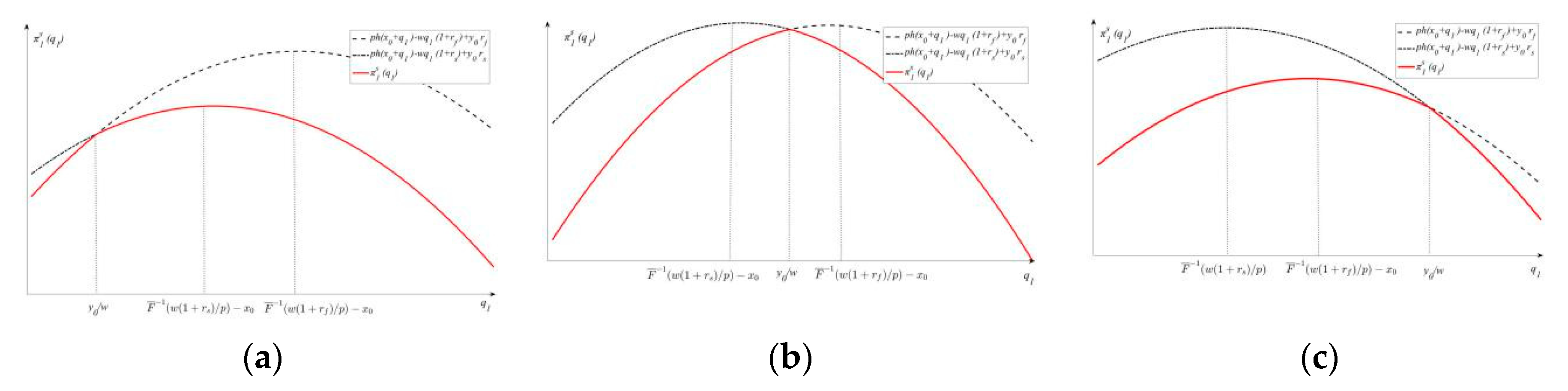
If
, the retailer cannot afford the purchase and need the supplier financing, it is his borrowing region. From
Figure 1a, the maximum point in
Case 1 can be reached, i.e.,
as (25a);
If
, the retailer will use all his equity capital to make purchases, that is to say, this is his all equity capital use region. From
Figure 1b, the retailer’s optimal order quantity is the intersection of the curves under two above cases, i.e.,
as (25b);
If
, the retailer has sufficient funds and only uses his partial equity capital to pay orders and gets risk-free investment with remaining capital. This is his partial equity capital use with risk-free investment region. From
Figure 1c, the maximum point in
Case 2 can be reached, i.e.,
as (25c). □
Different from the single-period bank financing problem with only single optimal solution, it can be seen from Theorem 2 that the retailer’s optimal strategy is characterized by two threshold values, which divide the ordering decision space into three regions to guide financing, operational, and investment decisions. Similarly, the supplier equilibrium under single-period supplier financing can be drawn by the discussion of retailer’s three initial inventory discount regions as THEOREM 4:
Theorem 4. Under supplier financing, the three regions divided by retailer’s initial discount inventory correspond to an optimal wholesale price, respectively. When in all equity capital use region, increases with w; when in partial equity capital use with risk-free investment region, ; when in partial equity capital use with risk-free investment region, ; when retailer borrows without bankruptcy, ; when retailer borrows with bankruptcy, .
Proof. Similar to the game equilibrium under single-period bank financing in Theorem 2, we discuss the three different regions of the retailer’s initial inventory discount separately based on the results in Theorem 3:
When in retailer’s all equity capital use region
, the retailer will pay his purchase in advance at the beginning of the sales season, and the supplier can use this early payment for risk-free investment similar to bank financing. The supplier’s expected terminal profit
is as following:
According to Theorem 3, bring
into Equation (32) and derive the supplier’s end-of-term profit function from
w, we have:
It can be seen that the supplier’s expected terminal profit is increasing with the respect of wholesale price without the optimal wholesale price in retailer’s all equity capital use region.
When in retailer’s partial equity capital use with risk-free investment region:
, the supplier can still use retailer’s early payment for risk-free investment similar to the above case, which follows the supplier’s expected terminal profit
as Equation (32). According to Theorem 3,
in partial equity capital use with risk-free investment region. Based on the implicit function theorem, we get the reaction function of
and
:
By deriving the supplier’s end-of-term profit function from
w, we have:
Let
, we obtain the supplier’s optimal wholesale price in retailer’s in partial equity capital use with risk-free investment region:
When in retailer’s borrowing region:
, the supplier uses retailer’s partial early payment for risk-free investment
. As the creditor, the supplier’s terminal expected terminal cash flow via financing the retailer follows Equation (9). The supplier’s expected terminal profit
under supplier financing as Equation (38):
When the retailer is not bankrupt,
, i.e.,
, Equation (38) can be simplified as (39):
According to Theorem 3, in borrowing region
. Based on the implicit function theorem, we get the reaction function of
and
:
By deriving the supplier’s end-of-term profit function from w, we have:
Let
, we obtain the supplier’s optimal wholesale price in retailer’s borrowing without bankruptcy region:
On the other side, when the retailer is bankrupt,
, i.e.,
, Equation (38) can be simplified as (43) with its first order differential condition as (44):
Substitute Equation (40) into (44) and let = 0, we have . In borrowing region, it satisfies the retailer’s first-order condition as (29), i.e., . Therefore, the supplier’s optimal wholesale price in retailer’s bankruptcy region satisfies: . □
4.3. Performance Comparison between Bank Financing and Supplier Financing
In the above theorems, we have obtained the retailer’s ordering strategy and the corresponding supplier’s equilibrium under bank financing and supplier financing respectively. In Theorem 5 we compare the supply chain performance under different financing decisions based on the above optimal order quantity and corresponding optimal wholesale price. It proves that trade credit cannot fully coordinate the supply chain compared with the centralized supply chain without financial constraints, but it still improves the supply chain performance compared with bank financing.
Theorem 5. When the financial-constrained retailer does not go bankrupt, the supply chain performance under supplier financing is better than that under bank financing, but it still cannot fully coordinate the supply chain unlike the non-financial constrained centralized supply chain, which means the retailer’s optimal order quantity increases in turn under bank financing, supplier financing and the centralized supply chain without financial constraints, i.e., .
Proof. First, we will prove the supply chain performance under supplier financing is better than that under bank financing, i.e., .
Substituting Equation (18) into (23) and after simplification we have:
Under supplier financing, we should consider the retailer’s borrowing region, for the convenience of comparison, we only discuss the non-bankruptcy case. Similarly, according to Equation (25a) and (37), we have:
According to
Section 3.2, demand distributions subject to an increasing failure rate (IFR), i.e., let
,
. We define
as the function of
which satisfies
and solve the first derivative for it:
From Equation (47), it can be seen that
decreases with the respect of
. Substitute
and
into
, we have:
Assume
, then
, which means Equation (48) holds:
From Equation (48), we have . As decreases with respect of , when , there exists which is in contradiction with derived from (48).Therefore, holds.
Next we prove that
. For a centralized supply chain, because it is directly in touch with market demand and does not need to distribute, its overall profit
is satisfied Equation (49) with its first order differential condition as (50):
Let
, we have the centralized supply chain’s optimal order quantity as (51):
According to
Section 3.2, we have
, which means
.
In conclusion, holds. □
5. Two-Period Dynamic Financing Problem
On the basis of the above section, we extend the single-period financing model to the two-period situation, considering the dynamic inventory and capital flow to analyze operational and financing decisions. When a retailer places an order with a supplier in multiple ordering seasons, inventory and liquidity of each period can be passed to the next period, which form a multi-period Stackelberg game between the supplier and the retailer. The general multi-period model has been described in
Section 3.3. Next in order to simplify the calculation, we take the two-period situation as an example to analyze retailer’s ordering strategy and multi-period game equilibrium.
5.1. Two-period Bank Financing Problem
Recall our single-period static financing model under bank financing with retailer’s optimal ordering strategy and supplier’s optimal wholesale price, this subsection considers the two-period case under bank financing to analyze how to maximize the terminal cumulative profits at the end of the second periods with the perspective of the retailer and the supplier, respectively.
According to Equation (3), we get the retailer’s profit in the second period under the two-period bank financing scenario by replacing parameter
t with 2 and general interest rate r with
:
According to the conclusion of one-period financing model, if only the second period is discussed, i.e., t = 2 and
is fixed, it can be regarded as a one-period problem, which can be obtained from Theorem 1:
Let denote
to represent the retailer’s base-stock level in the second period under bank financing, which is composed of the retailer’s initial inventory at the beginning of the second period
and his optimal ordering quantity in the second period
. After simplification of Equation (53), we have:
The retailer’s optimal order quantity satisfies Equation (55):
According to Bellman’s principle of optimality mentioned by Kogan [
36], no matter what the past state and decision of the process are, the remaining decision must constitute the optimal strategy for the state formed by the previous decision. Therefore, when considering the retailer’s decision in the first period, the decision in the second period can reach the optimal order quantity
.
Since the retailer’s cash flow and inventory are uncertain at the beginning of the second period, it is necessary to discuss the retailer’s different asset situations after the first sales period, which will determine the retailer needs to order product or make a bank loan or not at the second period.
Case 1:
When the retailer needs to order products with the bank financing at the second period, it implies the following two constraints:
and
. After simplification, we have:
Let
, from (56) and (57), it can be concluded that the stochastic demand in the first period
needs to meet:
Equation (52) can be written as follows:
In the two-period scenario, Equation (5) shows that the boundary condition satisfies
so a retailer’s profit function in the second period of
Case 1 can also be expressed as the retailer’s expected cumulative profit-to-go calculated from the second period as follows:
When
is determined,
is determined, which can be regarded as a single-period case. When there are two periods with unknown
,
is uncertain. Because of the retailer’s inventory transfer equation as Equation (1), the above formula can be rewritten as follows:
Case 2:
When the retailer needs to order products without bank financing at the second period, it implies the following two constraints similar to Case 1: and .
Similar to
Case 1, it can be concluded that
needs to meet Equation (61):
Equation (52) can be written as follows:
Then we get the retailer’s expected cumulative profit-to-go calculated from the second period in
Case 2 as follows:
Case 3:
When the retailer need not order products from the supplier at the second period, it implies
, i.e.,
. Under this circumstance, Equation (52) can be written as follows:
Then we get the retailer’s expected cumulative profit-to-go calculated from the second period in
Case 3 as follows:
According to the above three cases which cover all the range regions of the demand in the first period, the retailer’s expected cumulative profit-to-go calculated from the second period can be written as following:
Based on Equation (4), we derive the retailer’s expected cumulative profit-to-go calculated from the first period:
In order to obtain the retailer’s optimal strategy in two-period bank financing situation, we analyze some properties of the retailer’s expected cumulative profit-to-go by Lemma 1.
Lemma 1. The retailer’s expected cumulative profit-to-go under two-period bank financing is concave with respect to .
Proof. Since
, we have
. According to A6, retailer have to order from the supplier and make loans from the bank at the beginning of the first period, which means the retailer’s expected terminal profit at the first period and its first-order differential condition is consistent with the single-period bank credit model in
Section 4.1 as Equations (16) and (17).
According to Equation (67), we have the simplified first-order differential condition of
as (68):
Then we get the second derivative of the retailer’s expected cumulative profit-to-go calculated from the first period:
Since it is known that , we come to the conclusion that the second derivative of the retailer’s expected cumulative profit-to-go calculated from the first period is negative, which means it is concave with respect to . □
According to Lemma 1, the retailer’s expected cumulative profit-to-go calculated from the first period is concave function. According to the nature of concave function, there must be an optimal order quantity to maximize the retailer’s expected cumulative profit-to-go. Theorem 6 will give the retailer’s optimal ordering strategy in two-period bank financing.
Theorem 6. Under the two-period bank financing with the assumption that the financial-constrained retailer need to order from the supplier and borrow from the bank at the beginning of the first period, the retailer’s optimal order quantity in the second period is consistent with that in the single period, i.e., and ; the retailer’s optimal order quantity in the first period is , in which is determined by Equation (70).
Proof. According to A6, the financial-constrained retailer need to order from the supplier and borrow from the bank at the beginning of the first period, i.e., and .
Since Lemma 1 has proved that the retailer’s expected cumulative profit-to-go
under two-period bank financing is concave with respect to
with a maximum point. According to Equation (68) in Lemma 1, we derive the retailer’s optimal first order condition by substituting
into Equation (68) and obtain Equation (70) after simplification:
In Equation (70), and .
Due to implicated by A6, the retailer’s optimal order quantity at the first period satisfies , in which can be determined by Equation (70). □
After solving the retailer’s problem under two-period bank financing, the supplier game equilibrium two-period bank financing can be drawn as Theorem 7:
Theorem 7. Under the two-period bank financing, the supplier’s optimal wholesale price in the second period is consistent with that in the single period, i.e., ; her optimal wholesale price in the first period is determined by Equations (73) and (74).
Proof. Similar to the supplier’s problem under the single-period bank financing analyzed in
Section 4.1, the supplier can use a retailer’s early payment for risk-free investment.
The cumulative profit-to-go calculated from the second period as follows:
From Theorem 2 and Theorem 6, it can be seen that
and
, let
. The supplier’s expected cumulative profit-to-go calculated from the first period as following:
The optimal first-order condition of supplier’s expected cumulative profit-to-go with respect of
as (73):
It means that the supplier’s optimal wholesale price satisfies Equation (73). According to Equation (68), we get the reaction function of
and
based on the implicit function theorem:
□
In above, it can be seen that the Stackelberg equilibrium under two-period bank financing is composed of the optimal policy matrix determined by Theorems 6 and 7.
5.2. Two-Period Supplier Financing Problem
This subsection considers the two-period case under supplier financing to analyze how to maximize the terminal cumulative profits at the end of the second periods with the perspective of the retailer and the supplier, respectively.
Similar to
Section 5.1, we will derive the retailer’s expected cumulative profit-to-go calculated from the first period and obtain its optimal first-order condition as Theorem 8.
Theorem 8. Under the two-period supplier financing with the assumption that the financial-constrained retailer need to order from the supplier and borrow from the supplier at the beginning of the first period, the retailer’s optimal order quantity in the second period is consistent with that in the single period, i.e., and ; the retailer’s optimal order quantity in the first period is , in which is determined by Equation (79).
Proof. From Theorem 3, let denote
represent the retailer’s base-stock level in the second period under supplier financing, we rewrite the above equation as follows:
The retailer’s optimal order quantity satisfies Equation (76):
Since the discussion of retailer’s different financing and operational decisions for his expected cumulative profit-to-go calculated from the second period is similar to
Section 5.1, which also analyzes three cases including ordering and borrowing scenario, ordering and non-borrowing scenario and non-ordering scenario, we omit the discussion procedure for the sake of brevity and derive the retailer’s expected cumulative profit-to-go calculated from the second period as follows:
It is noted that , we have .
Similar to Lemma 1, we come to the conclusion that the second derivative of
is negative, which means it is concave with respect to
. Therefore there must be a
to maximize the retailer’s expected cumulative profit-to-go calculated from the first period
. After some simplification, we obtain the optimal first condition as following:
In (78), and .
Due to implicated by A6, the retailer’s optimal order quantity at the first period satisfies , in which can be determined by Equation (78). □
After solving the retailer’s problem under two-period supplier financing, the supplier game equilibrium of two-period bank financing can be described by Theorem 9:
Theorem 9. Under the two-period supplier financing, the supplier’s optimal wholesale price in the second period is consistent with that in the single period, which can be seen in Theorem 4. Her optimal wholesale price in the first period is determined by Equation (82).
Proof. According to Theorem 4, we can know that: when retailer use his partial equity capital with risk-free investment, ; when retailer borrows without bankruptcy, ; when retailer borrows with bankruptcy, .
According to the three cases which cover all the range regions of the demand in the first period which is similar to the retailer problem, the supplier’s expected cumulative profit-to-go calculated from the second period can be written as Equation (79) and the supplier’s total expected cumulative profit-to-go calculated from the first period can be written as Equation (80):
After simplification, we have the first-order differential condition of
as (81):
Let
and after simplification, it can be seen that the supplier’s optimal wholesale price satisfies Equation (82):
In (82), .
According to Equation (78), we get the reaction function of
and
based on the implicit function theorem:
□
In above, it can be seen that the Stackelberg equilibrium under two-period supplier financing is composed of the optimal policy matrix determined by Theorems 8 and 9.
6. Numerical Analysis
This section will simulate bank financing and supplier financing model under the single-period and two-period scenarios mentioned in the respective sections above, We illustrate the advantages of supplier financing compared with bank financing and the improvement of supply chain performance from the perspective of the retailer and the supplier through practical numerical analysis.
First of all, we make some assumptions and explanations on the basic parameters involved in this paper. We assume that the stochastic demand are subject to a uniform distribution from 0 to 200, i.e., D~U(0,200). The probability density function of the stochastic demand satisfies: . The probability distribution function satisfies: .
Since A6 assumes that the retailer is capital-constrained in the first period in a multi-period scenario. Therefore, in the absence of special instructions, , , , , , , .
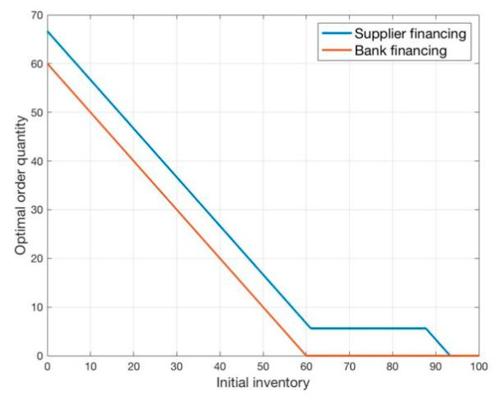
According to Theorems 1–4, the trend of the retailer’s optimal order quantity under the single-period bank financing and supplier financing with the change of
is shown in
Figure 2. It shows that under the single-period bank financing, when the retailer’s initial inventory
,
decreases with the initial inventory
, and when
, the inventory at the beginning of this period has exceeded the retailer’s base-stock level under bank financing so that the retailer doesn’t need to order anymore. Under the single-period supplier financing, when
,
, it is in the retailer’s borrowing region,
decreases with the increase of
. When
, it is in the retailer’s all equity capital use region,
does not change with the
changes. When
, it is in the partial equity capital use with risk-free investment region,
decreases with the increase of
. When
, the initial inventory has exceeded the retailer’s base-stock level under supplier financing so that the retailer doesn’t need to order anymore. Comparing bank financing with supplier financing in
Figure 2, it can be seen that under the same initial inventory setting, the retailer’s optimal order quantity under single-period supplier financing will be higher than bank financing.
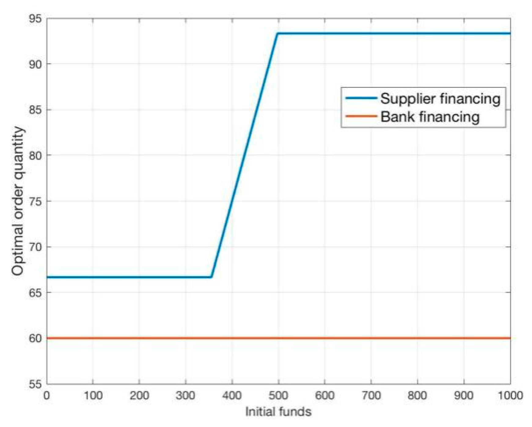
When
is fixed, the trend of the retailer’s optimal order quantity under the single-period bank financing and supplier financing with the change of
is shown in
Figure 3. It can be seen from
Figure 3 that under the single-period bank financing, the retailer’s optimal order quantity has nothing to do with the initial cash flow
, and the optimal order quantity is maintained at 60, which is consistent with the conclusion driven in Theorem 1 that when bank credit are price competitive, the retailer’s ordering strategy under the single-period bank financing is not affected by his capital constraints. In the case of single-period supplier financing, it can be seen from Theorem 3 that the retailer’s wealth can be divided into three regions according to its initial discount inventory, which is also reflected in
Figure 3, when
, the retailer’s wealth status was poor and it is in its borrowing area. At this time, the optimal order quantity was maintained at 66.67, which is consistent with the result of
in
Figure 2. When
, it is in the retailer’s all equity capital use region,
increases with
, which is also consistent to the conclusion of Theorem 3 that
. When
, it is in the partial equity capital use with risk-free investment region. At this time,
remains unchanged at 93.33. At the same time, compared with the optimal order quantity under bank financing and supplier financing, the order quantity of supplier financing is higher than bank financing, which also illustrates the conclusion of Theorem 5 that single-period supplier financing can increases overall supply chain performance compared with bank financing due to increased order quantities.
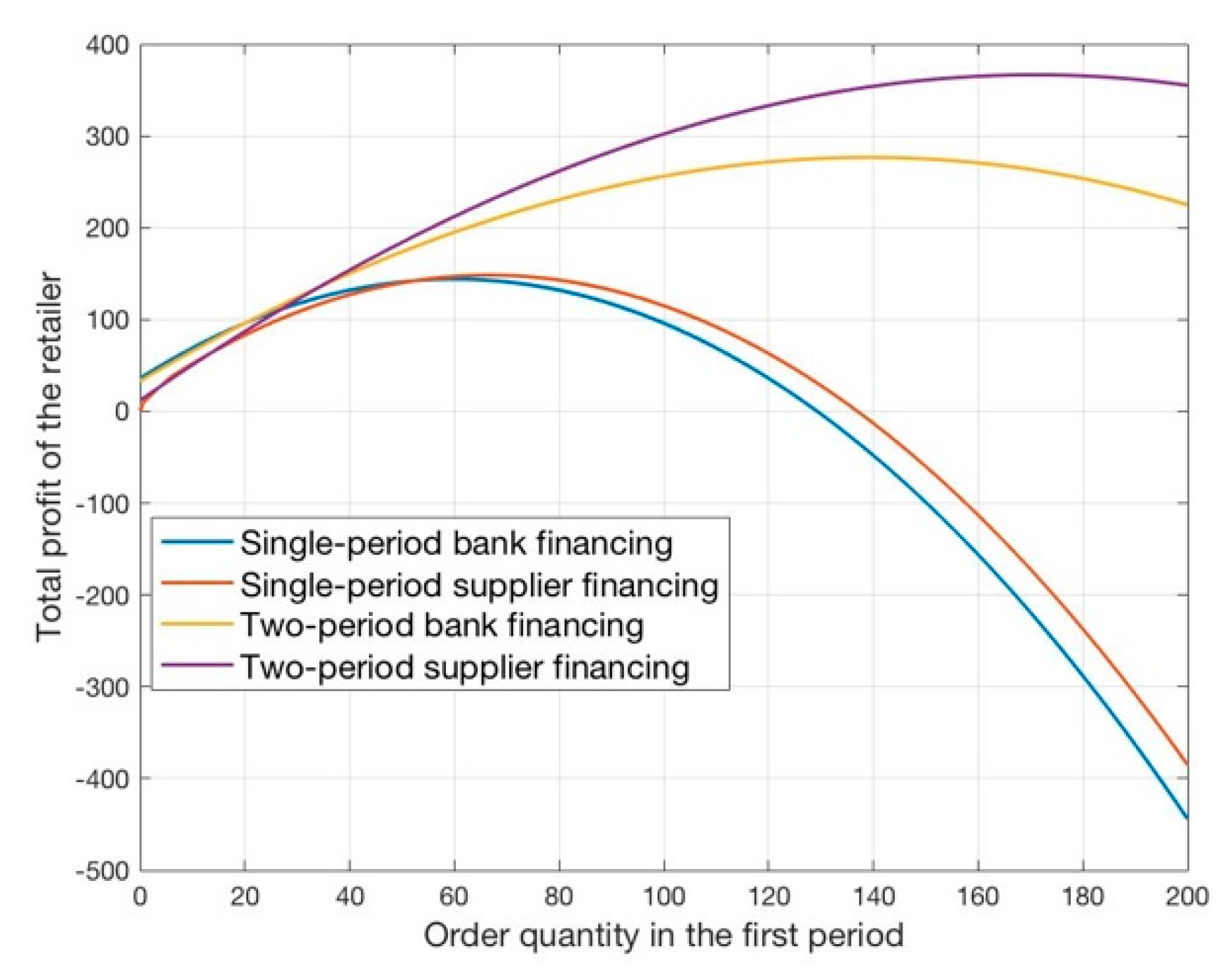
When
and
is fixed,
Figure 4 shows the retailer’s total profit curves with the respect of the order quantity of first period under bank financing and supplier financing in single-period and two-period scenarios. It can be seen from
Figure 4 that the retailer’s expected terminal profit functions under these four scenarios mentioned above are all concave with respect to the order quantity of first period as we prove in
Section 4 and
Section 5. Comparing the retailer’s expected terminal profit under single-period bank financing and supplier financing, when the order quantity is less than 52, the retailer’s profit of bank financing is higher than that of supplier financing, or retailer’s profit of supplier financing will higher than that of bank financing, and because in our initial setting,
and
are both higher than 52, which means that in this case, the retailer will select supplier financing that maximizes his terminal profit.
It also can be seen that the retailer’s two-period cumulative profit under supplier financing is higher than that of bank financing when the retailer chooses the optimal strategy. Compared with single-period and two-period settings, whether it is a two-period bank financing or a supplier financing, the retailer’s two-period cumulative profit is higher than the single-period situation. Especially the retailer’s two-period cumulative profit under supplier financing is 366.6 when , which is more than twice the retailer’s single-period terminal profit of 148.3 when , which means that the retailer will prefer two-period supplier-financing to maximize his cumulative profit.
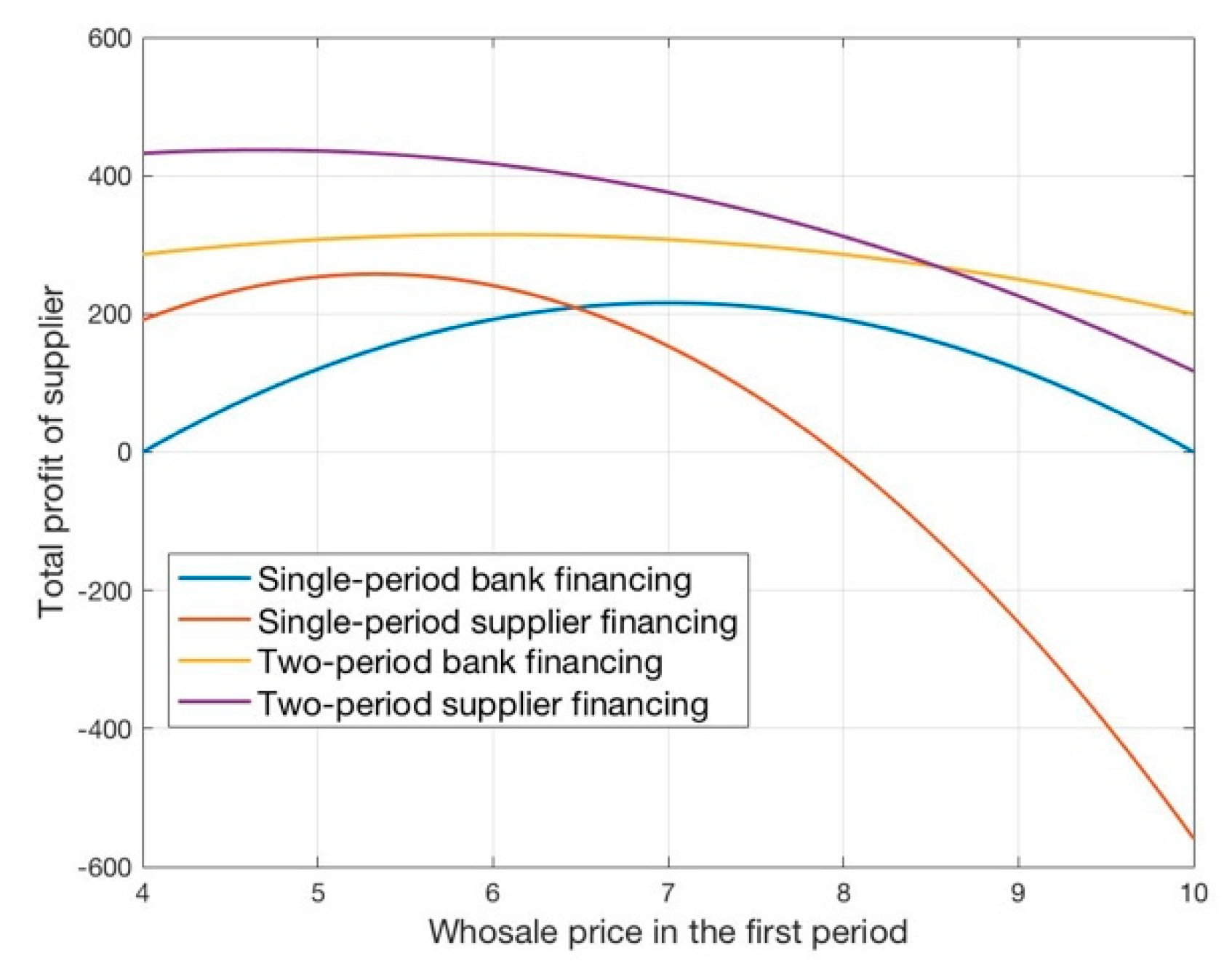
On the other side,
Figure 5 shows from the supplier’s perspective the impact of the first-period wholesale price on the supplier’s expected terminal profit under bank financing and supplier financing in single-period and two-period scenarios. Compared with the supplier’s expected terminal profit under single-period bank financing and supplier financing, it can be seen that when the wholesale price is less than 6.47, the supplier’s expected terminal profit of supplier financing is higher than the bank financing, on the contrary, the bank financing will be better for the supplier. This is because when the wholesale price is low, the retailer’s optimal order quantity increases. If the retailer chooses the supplier financing, the supplier can compensate for the loss of profits caused by the reduction of the wholesale price or even bring higher profits by trade credit obligation and increasing order quantity. However, when the wholesale price is too high, the retailer’s order quantity will decrease, which leads to a decrease in the supplier’s terminal profit. It also can be seen from
Figure 5 that
, which is lower than
and at that time the supplier’s expected terminal profit under supplier financing is 257.7, which is higher than that of bank financing, which is 216.
Figure 5 also shows that the supplier’s two-period cumulative profit under supplier financing is higher than that of bank financing when the retailer chooses the optimal strategy. In addition, unless under supplier financing or bank financing, supplier’s two-period cumulative profits are both higher than that in the single-period situation. Similar to retailer’s respective, supplier’s cumulative profit under the two-period supplier financing is more than double of single-period supplier’s expected terminal profit, which means that the supplier will also choose to financing the retailer in two-period in order to maximize her own final profit.
Figure 4 and
Figure 5 illustrates the superiority of supplier financing compared to bank financing and the two-period setting compared to single-period setting from the perspective of the retailer and the supplier respectively.
7. Conclusions
In this paper, we mainly study the single-period and two-period financing game of the capital-constrained supply chain with bank credit and trade credit. By using the game theory, we analyze the optimal operational and financial strategies of the supplier and the retailer.
Firstly, we establish the Stackelberg game with the supplier as the leader and introduce dynamic inventory and capital flow to build multi-period general financing model consisting of inventory and cash-flow transfer equation and the expected cumulative profit-to-go from period t to period T.
Secondly, in the single-period static financing model, we prove that the retailer’s decision under bank financing is not subject to financial constraints, which can be regarded as unconstrained newsvendor model. In terms of single-period trade credit, we divide the retailer’s initial inventory and capital into three different wealth regions and discuss the retailer’s optimal ordering strategies and the supplier’s game equilibrium of different wealth regions. We prove that the trade credit can improve the supply chain’s performance rather than bank credit, but it still cannot fully coordinate the supply chain unlike the non-financial constrained centralized supply chain,.
Thirdly, we extend the single-period financing model to the multi-period dynamic financing model and take the two-period setting as an example. We discuss the retailer’s different asset situations after the first sales period to obtain the optimal policy matrix of the retailer and the supplier under trade credit and bank credit.
Finally, numerical analysis illustrates that two-period trade credit can improve the performance of the supply chain and it is the best choice both for the retailer and the supplier, which provides support for our theoretical analysis.
This work still has some limitations. We have not explained the cause of financial constraints which may be asymmetric distribution of information or exogenous shocks, which may be lead to the result that a generic reference to "constraints" can impair the generalization of results. On the other hand, we neglect potential connections between subsequent periods caused by information updating and creditor’s learning behavior under multi-period supply chain financing, which will have an impact on the creditor’s financing decisions, such as interest rates of bank and supplier, while the learning effect may ease financial constraints and lead to a new game equilibrium.
There are some logical extensions to this study. First, supply chain contracts such as revenue sharing contract or quantity discount contract can be introduced to coordinate the supply chain. Second, the number of periods can be considered to analyze their effects on multi-period game equilibrium. Third, the information asymmetries theoretical framework can be introduced to discuss how does trade credit alleviate information problems and the impact of information updating and creditor’s learning behavior on multi-period creditor’s financing decisions can be discussed. Finally, besides the order quantity and wholesale price, the credit interest rate of the bank and supplier may be another factor with some interesting properties of the capital-constrained supply chain.


