Dantzig Type Optimization Method with Applications to Portfolio Selection

1
Department of Statistics, Sungkyunkwan University, Jongno-gu, Seoul 03063, Korea
2
Department of Mathematics and Computational Science & Engineering, Yonsei University, 50 Yonsei-ro Seodaemun-gu, Seoul 03722, Korea
3
School of Liberal Arts, Seoul National University of Science and Technology, Seoul 01811, Korea
*
Author to whom correspondence should be addressed.
†
These authors contributed equally to this work.
Sustainability 2019, 11(11), 3216; https://doi.org/10.3390/su11113216
Submission received: 8 May 2019
/
Revised: 3 June 2019
/
Accepted: 5 June 2019
/
Published: 10 June 2019
(This article belongs to the Section Economic and Business Aspects of Sustainability)
Abstract
:This paper investigates a novel optimization problem motivated by sparse, sustainable and stable portfolio selection. The existing benchmark portfolio via the Dantzig type optimization is used to construct a sparse, sustainable and stable portfolio. Based on the formulations, this paper proposes two portfolio selection methods, west and north portfolio selection, and investigates their empirical properties. Numerical results presented for 12 datasets and various simulated data show that the west selection can reduce risk, and the north selection may outperform the benchmark as to risk-adjusted returns (based on, e.g., information ratio and Sharpe ratio).
1. Introduction
The mean–variance portfolio optimization theory [1] has been improved in various ways due to its usefulness. The mean–variance portfolio optimization theory is based on the assumption that investors want high returns with low risk. However, in practice, it is extremely difficult to implement [2,3]. One main reason for the implementation difficulty is the estimation errors of the covariance matrix and the expected return. It is well known that Markowitz portfolios can be heavily affected by estimation error, tend to perform badly out-of-sample, and result in allocations with very unstable and extreme asset weights [4,5]. As extant financial literature has shown repeatedly, using sample estimates cannot provide reliable out-of-sample asset allotments in real implementations [2]. DeMiguel et al. [5] demonstrated that the estimated window required for a sample-based mean–variance portfolio to exceed the equally-weighted portfolio is approximately 6000 months for a portfolio of 50 assets. In reality, however, one is never in possession of sufficient data to estimate the covariance matrix and expected returns with a desired degree of precision. As Michaud [6] indicated, inverting ill-conditioned covariance matrices drastically amplifies estimation errors in the optimization step. Consequently, this can lead to poor out-of-sample performances of sample-based mean–variance portfolios.
Many studies have been performed to overcome these implementation difficulties through improving parameter estimation or constraining portfolio weights. Specifically, to obtain better covariance matrix estimations, one can impose some factor structures [7,8], use graphical models [9], or take a weighted average of covariance matrix estimators [10,11]. For constraining the portfolio weights, short sale constraints [12,13] and various regularization methods [14,15] have been proposed. To obtain sparse portfolios (i.e., portfolios consisting of a few assets), convex relaxation approaches using regularization or their variations have been developed [15,16,17]. Including these regularization terms in the optimization problem can assist to bound optimization errors and deal with ill-conditioned covariance matrices, and hence enhance the robustness of the portfolio with respect to estimation errors [5,16,17,18].
In this paper, an approach by constraining the portfolio weights using a benchmark portfolio is proposed. The aim of this paper is to push the benchmark to an efficient frontier to obtain a better optimal portfolio. Specifically, for some , the investors invest in a few assets determined by the proposed Dantzig type method and invest in the benchmark. The main idea is similar to the methods in Park et al. [19]. As in Park et al. [19], this paper considers two methods of portfolio selection, west selection and north selection, based on a few assets in the market using a variance as risk. The west selection pushes a benchmark to the west, and the north selection pushes a benchmark to the north. The west selection is a risk-based portfolio, which requires estimation of the covariance matrix of asset returns. On the contrary, the north selection is both return and risk-based, i.e., it requires both the covariance matrix and expected returns estimations.
The main differences of the current work compared with the work of Park et al. [19] are as follows: (1) the proposed portfolios utilize a variance (quadratic term) as portfolio risk while Park et al. [19] utilizes other risk measures (linear term); (2) the proposed optimizations are proven to be semidefinite programming problems as in Theorem 1, thus can be efficiently solved using a semidefinite programming solver with convergence guarantees; and (3) the sensitivity of key parameters of the proposed optimization problems is analyzed, as can be found in Theorems 3 and 5, suggesting that the proposed portfolio selections are insensitive to the regularization parameters under reasonable candidate sets of parameters.
From a pragmatic perspective, the proposed approach can be easily modified and extended. For example, one can use various risks and objective functions depending on investors’ utility of the portfolio return and risk. Two different benchmarks, the equally-weighted portfolio and the GMVP (global minimum variance portfolio) formed from assets in the market are considered. To measure performance relative to the benchmark, various measures such as cumulative returns, the information ratio, and kurtosis are also considered.
Literature Reviews
Recently, there have been many studies to obtain the strategy for sustainable and effective portfolio selection with various approaches [20,21,22,23]. In this paper, a well-established benchmark (e.g., Dow 30 index), which offers sustainable and stable risk-return profiles with low costs, is used to propose an effective strategy for constructing a portfolio. The essential idea of the proposed method can be also found in the index tracking problem in the works of Roll [24] and Jorion [25]. However, a crucial difference exists between their methods and the west selection from two financial standpoints. Unlike the proposed portfolios, the optimal portfolio weights of Roll [24] and Jorion [25] are not necessarily sparse and stable over time, which can generate significant costs for investors. It is desirable to make a portfolio with sparse, sustainable and stable portfolio selection to decrease both management and transaction costs [26]. From a statistical view, sparse asset selection can be efficient for reducing estimation errors when the number of parameters for the optimization increases. Another related portfolio selection method is enhanced indexation (EI) [27,28,29,30,31,32,33], which attempts to attain high returns of constructed portfolios at the same time controlling risk. Specifically, EI-based optimizations utilizing stochastic dominance criteria are considered in several studies [34,35]. It is worth mentioning that, in multi-stage production models [36,37,38], the budget is also a bigger issue for industry sectors [39]. Sarkar [39] developed a mathematical and analytical approach for the management of defective items, which aims to diminish wastes for minimizing the total cost.
For selecting the stocks to be included, a convex penalty, i.e., the Lasso [40], which often behaves similarly to the penalty, is used. Index tracking approaches exist that use a subset of stocks by directly imposing cardinality constraints. The problem of selecting stocks to be included in the tracking portfolio is NP-hard [41]. Many heuristic algorithms have been developed to identify practical solutions that are close to the global optimum: Gilli and Kellezi [42] presented a threshold-accepting heuristic algorithm demonstrating that it constitutes an efficient optimization technique for index tracking problems with a small number of stocks in the benchmark index; Beasley et al. [43] presented an evolutionary heuristic algorithm for the solution of the index tracking problem by including a constraint limiting the number of stocks, as well as transaction costs; Ruiz-Torrubiano and Suárez [41] proposed a hybrid strategy that combines an evolutionary algorithm with quadratic programming; and Ni and Wang [44] proposed a heuristic-searching approach that is based on a hybrid genetic algorithm with a self-adaptive evolving mechanism.
Similar to Sarkar [39], we construct a table to better present the characteristics and contributions of the proposed methods. Table 1 summarizes the model/method contributions of the proposed methods and the other portfolio selection methods, where the names of methods or authors and the corresponding literature can be found in the “Method” column. The “Optimization” column contains four factors considered in the optimization problems, the “Parameter selection” column is separated into two cases (Cross-validation and Fixed) based on the way of choosing regularization parameters in the corresponding optimization problem, and the “Performances” column includes the four measures (Return, Skewness, Turnovers, and Sharpe Ratio) used when quantifying out-of-sample performance of the portfolios. For each method, when the method corresponds to a specific factor, the corresponding factor is checked (✓), e.g., north selection is checked on the “Cross-validation” in the “Parameter selection” column because north selection utilizes 10-fold cross validation when determining regularization parameters.
It can be seen that the north selection simultaneously consider return, risk, sparsity, and stability in the optimization problems, while the other methods only incorporate at most three factors in their optimizations, suggesting that the north selection can be favorable to investors who want a sparse, stable, and profitable portfolio. Regarding parameter selection, the proposed methods utilize the cross-validation, which is known to be more developed method than when a fixed parameter is used in the implementation. To quantify the performances of the methods, it would be good to utilize as many measures as possible because each measure captures different aspects of portfolio. In this regard, the proposed methods are more comprehensively evaluated compared to other methods in the literature.
The remainder of the paper is organized as follows. Section 2 develops the proposed methods and investigate their theoretical properties such as convergence of the algorithms and sensitivity analysis of the main parameters in the proposed optimization problems. Section 3 provides the implementation procedures of the proposed methods. Section 4 shows various out-of-sample performances of the proposed portfolios relative to the benchmark using several real datasets as well as simulated data. Section 5 gives the conclusion.
2. Portfolio Selection
Suppose that the return on a portfolio can be described as a sum of p risky asset returns:
where , asset i has return , and the proportion of capital that is invested in the asset i is . Denote the portfolio weights by and the asset returns . Denote expected returns of p assets by , i.e., , and to denote the covariance matrix of asset returns. Let and be the estimates of and ∑, respectively. Thus, is the estimate of μ. Hence, the estimate of returns and variance for the portfolio can be expressed as respectively. Throughout the paper, for a vector v, define For any numbers a and b with a < b, let Denote the identity matrix by I.
2.1. Intuitive Ideas
Let v be a benchmark portfolio, which satisfies , where is a vector of all ones. Consider the portfolio w in which the investors invest in the benchmark v and in the stocks that make up the benchmark. Then, the portfolio w can be represented as , where represents the deviation portion from . Here, the aim is to find the and that provide a portfolio w with higher return or lower risk compared to the benchmark v. Here, sparsity and stability of selected assets in across times are desirable for controlling both management and transaction costs; sparsity is related to management costs, and stability of the portfolio is related to transaction costs [26]. Transaction costs are one critical factor to be considered in the portfolio optimization problem [14].
For fixed , one can consider the following problem to minimize the total risk of the portfolio :
for some , where the penalty, called Lasso [17,40], is a convex penalty, which often behaves similarly to the penalty. However, since Equation (1) does not exploit the information of obtained from the previous time, the solution to Equation (1) does not guarantee a stable solution in the sense that may have totally different selected assets (i.e., assets with non-zero weights) compared to those of the previous time.
To obtain sparse, sustainable and stable portfolio selection, one can consider the following optimization:
where is the weight of the ith asset during the former time. The second constraint in Equation (2) is essentially the same as the adaptive Lasso [45], which plays a crucial role in the sparse, sustainable, and stable asset selection by adaptively shrinking coefficients based on the corresponding weight at the previous time, so that assets with larger weights at the previous time tend to have larger weights at the current time.
2.2. West Selection
The portfolio in Equation (2), based on the adaptive Lasso, provides a more stable asset selection compared to that in Equation (1) based on the Lasso. Since the term can be arbitrarily large, may have a wide range of possible values and it can require a long computation time to determine an appropriate . To overcome this implementation difficulty, the objective and the constraint term in Equation (2) are interchanged, and Equation (2) in a mathematically equivalent way is reformulated. This is first method, west selection: for fixed and ,
where is an estimated benchmark risk. To avoid division by zero in Equation (3), , where is the weight of the ith asset during the former time, is used. This small adjustment procedure is standard and can be found in many studies related to adaptive Lasso, e.g., those of Zou and Zhang [46] and Chatterjee and Lahiri [47].
The optimization in Equation (3) then updates the portfolio on a monthly basis, while restricting variations from the former time. Note that , the estimate of the covariance matrix at time t, by using previous one-year daily data from time point t, is obtained. See Section 2.6 for a discussion about the covariance matrix estimator. The algorithm is summarized as follows:
| Algorithm 1: West selection. |
Input: Initial time (month) and . Outputs: The deviations vectors at months . Repeat until . Step 1: Step 2: Update , such that . Obtain , the solution to Equation (3), with the specified , , , and . Step 3:. |
The parameters and in Step 1 via 10-fold cross validation at each time are chosen for the implementations. See Section 2.5 for details. The optimization problem in Equation (3) is similar to the Dantzig type optimization problems [48,49] in that it minimizes the penalty subject to some constraints. The sample variance of the benchmark return computed from the previous one-year data for is used. Note that controls the total portfolio risk, and is easily interpreted in comparison with the constraint in Equation (2). It controls the risk of the target portfolio with respect to the benchmark by c3. For example, if c3 = 1, the candidate portfolios are the ones with smaller risk compared to the benchmark, i.e., push of the benchmark to the left (i.e., west) on the risk-return plane is conducted.
2.3. North Selection
In this subsection, another portfolio selection method, which pushes the benchmark in the north direction, is considered. An additional constraint to the west selection in Equation (3) is as follows: for fixed and ,
where is an estimated expected return of the benchmark portfolio v, and is determined in a way similar to Equation (3). The sample mean of the benchmark return obtained from the previous one-year data for is used. The role of the third constraint is to push the v in the north direction by to achieve higher expected return compared to v. Note that we obtain
and , the estimates of the covariance matrix and expected returns at time t, respectively, by using the previous one-year daily data from time point t. The algorithm is summarized as follows:
| Algorithm 2: North selection. |
Input: Initial time point (month) and . Outputs: The deviations vectors at months . Repeat until . Step 1: Obtain , the solution to Equation (4), with the specified , , , , and . Step 2: Update such that . Step 3:. |
The parameters and in Step 1 are chosen via 10-fold cross validation at each time. See Section 2.5 for details. Notice that Equations (3) and (4) are not readily applicable when the benchmark weight v is not available in advance. In this case, the terms and by using the estimate of the benchmark portfolio risk and the estimate of the cross-covariance of the benchmark portfolio and the other p assets are substituted, respectively. More specifically, since the term represents a variance of the benchmark return, we replace this term with . Since the term by the sample cross-covariances of the benchmark return and the other p asset returns are replaced.
Since the proposed optimizations in Equations (3) and (4) are convex, these problems can be solved using convex optimization packages. Since Equations (3) and (4) are semidefinite programming problems, as proved in Theorem 1, any semidefinite programming solver guarantees a convergence of the algorithm. Specifically, the SDPT3 solver (Semidefinite programming solver) in CVX [50] is used in the implementation.
Theorem 1.
The optimization problems in Equations (3) and (4) are semidefinite programming problems, respectively.
Proof.
See Appendix A. □
2.4. Properties of West and North Selections
This section investigates some properties of west and north selections. Theorem 2 shows that the west selection is the GMVP with some regularized covariance matrix. All the proofs are deferred to Appendix A.
Theorem 2.
The west selection (i.e., is the solution to Equation (3)) is the solution of the below global minimum variance optimization problem:
Here, is a regularized sample covariance matrix, where and g is the sub-gradient of computed at .
Note that Ledoit and Wolf [11] proposed replacing the sample covariance matrix with a weighted sum of the sample covariance matrix and a low-variance target estimator, such as the identity matrix and the covariance matrix obtained from estimating a 1-factor model with the market as the factor. The regularized covariance matrix in Theorem 2 is also the weighted sum of the covariance estimate and the rank-two matrix. When the shrinkage method [51] is used for as described in Section 2.6, i.e., for the sample covariance matrix and , the west selection in Equation (3) can be described as the minimum-variance portfolio with the regularized covariance matrix with the weighted sum of the three matrices: the sample covariance matrix; the structured rank-two matrix; and the identity matrix.
Note that sensitivity of the key parameters of the optimization problem is one of the important factors because determining parameters is critical in implementations. Theorem 3 shows the sensitivity of the regularization parameter in the optimization problem in Equation (3).
Theorem 3.
For fixed , let and be the solutions to Equation (3) with regularization parameters and , respectively, where . Then, it holds that
where
Theorem 3 gives a sensitivity of in the west selection problem, which suggests that differences of two west portfolios with the ϵ-difference in are bounded by - and ϵ-orders in terms of the Euclidean distance and the estimated risk, respectively. As a reasonable candidate set of is between 0 and 1 as in Section 2.5, Theorem 3 suggests that the candidate west portfolios are different at most a constant order even when p is large. That is, investors do not have to suffer from the choices of as long as the reasonable candidate sets of is considered.
Theorem 4 shows that the north selection is also the GMVP with some regularized covariance matrix.
Theorem 4.
The north selection (i.e., is the solution to Equation (4)) is the solution to the following global minimum variance optimization problem:
where the regularized sample covariance matrix is given by
where
and λ3 and λ4 are Lagrangian parameters, and g is the sub-gradient ofcomputed at
Theorem 4 implies that, when the risk constraint in Equation (4) is binding, i.e., in Equation (5), the north selection problem in Equation (4) is the minimum-variance problem with the covariance matrix The matrix can be interpreted as that of in the west selection method.
Theorem 5 gives a sensitivity of c4 in the north selection problem, which suggests that differences of two north portfolios with the e-difference in c4 are bounded by e-order in terms of the estimated return. Since a reasonable candidate set of c4 is between 0 and 1 as in Section 2.5, Theorem 5 implies that the considered north portfolios are different at most a constant order in terms of estimated return even when p is large. This suggests that the north selection could be attractive to investors who prefer stable model selection with respect to change of regularization parameters.
Theorem 5.
For fixed , let and be the solutions to Equation (4) with regularization parameters and , respectively, where . Then, it holds that
where is the estimated return of the portfolio .
2.5. Determining the Regularization Parameters
Note that the west and north selections can be infeasible for some and , respectively. Due to the constraint , Equation (3) can be infeasible for small . More specifically, it is easily deduced that the optimization problem in Equation (3) is infeasible when
where is the minimum eigenvalue of . Similarly, Equation (4) can be also infeasible when is sufficiently large. Equation (4) is infeasible when
In the in-sample window, α, , and using the 10-fold cross validation are determined. The former one-year daily returns into 10 most equal-sized subsets are randomly divided. Then, nine subsets as a training set to construct a portfolio are used, and treating remaining one subset as a validation set such that the mean return or Sharpe ratio of the constructed portfolio is calculated over the validation set. The reason for considering the two different criteria is to check that these parameters can be successfully chosen utilizing reasonable cross-validation criteria function. These cross-validation scores are averaged over 10 validations sets for each set or , and the set with the highest score is chosen. The α is selected from , while the and are chosen from and , respectively. When the west selection in the out-of-sample window is infeasible for the selected from the in-sample window, the is increased until Equation (3) is feasible. Similarly, if the north selection in the out-of-sample window is infeasible for the chosen , is decreased until Equation (4) is satisfied.
2.6. Estimation of Covariance Matrix
Mean–variance portfolio models require well-conditioned covariance matrix estimators of the asset returns, i.e., inverting the estimator does not amplify estimation error. Estimating the covariance matrix is challenging due to heavy-tailedness and the high dimensionality of asset return data. Specifically, the number of assets is usually much larger than the sample size. Some simple measures of correlation are often utilized in this covariance matrix, e.g., the RiskMetrics methodologies (JP Morgan) based on weighted moving averages and the sample covariance matrix. For large-dimensional covariance matrices, however, the sample covariance matrix is usually unstable and may not be invertible.
The orthogonal factor models by principal component analysis (PCA) have been also employed to simplify the process of producing these large covariance matrices [52]. Using PCA is computationally simple as it takes the univariate volatilities of the first few principal components of a system of risk factors and generates a full covariance matrix for the original system by a few components. The principal components can be used with standard volatility estimation methods [52], such as exponentially weighted moving averages (EWMA) or generalized autoregressive conditional heteroscedasticity (GARCH) [53,54], to produce large positive semi-definite covariance matrices.
To overcome the problem of dimensionality, structured covariance matrix estimators are also considered for asset return data. Fan [55] proposed estimators based on factor models by utilizing observable factors. Bai and Li [56] and Fan et al. [57] analyzed covariance matrix estimators based on latent factor models. Ledoit and Wolf [51] and Ledoit and Wolf [11] proposed to shrink the empirical covariance matrix towards highly structured covariance matrices, including the identity matrix, autoregressive covariance matrices, and one-factor-based covariance matrix estimators.
Among these covariance estimators, the shrinkage method [51] is used. In this sense, an optimal weighted average of an identity matrix I and the sample covariance matrix , i.e., for some is used. The results empirically show that this shrinkage method works well with the proposed method. The shrinkage method is suitable especially for high-dimensional data, and well-conditioned compared to the sample covariance matrix [11,51].
3. Implementation
This section provides the implementation details.
3.1. Computation
Since the proposed optimizations in Equations (3) and (4) are convex, they can be solved using convex optimization packages. CVX in Matlab was used. For each method, two performance measures (mean return and Sharpe ratio) were utilized as criterion functions in the 10-fold cross validation to determine regularization parameters α, , and , as described in Section 2.5. Based on the selection methods and the cross-validation criterion functions, the four different portfolios listed in Table 2 were considered. Specifically, W-R and W-S are two different west selection portfolio strategies using the return and Sharpe ratio in the cross-validation procedure, respectively, while N-R and N-S are two different north selection portfolio strategies.
3.2. Performance Measures of a Portfolio
Let be the asset return vector whose ith component is the return of the asset i at time t. Let denote the proposed portfolio at time t and denote the set of non-zero components in . The following out-of-sample performance measures when evaluating the performance of the portfolio over the monthly time periods from to T were used:
- Return: .
- Risk: .
- Sparsity: The proportion of the selected assets in for time t, i.e., , where is the number of the nonzero components in . Sparse asset selection in the portfolio optimization is important for investors because it controls management costs.
- Stability: Cardinality of set differences of the selected assets between two consecutive time points divided by p, i.e., . Here, represents the set difference of sets A and B. Stable asset selection is one of the important factors to consider as it is related to transaction costs.
- Turnover (trading volume): The average volume of the rebalancing trades across the assets over the trading dates, i.e., , where the benchmark as one available asset in the market is considered.
- Sharpe ratio: The ratio of the mean return to risk: . Larger Sharpe ratios indicate higher risk-adjusted returns.
- Kurtosis: The measure of the tailedness of the returns. A higher kurtosis is the result of infrequent extreme outliers or deviations:
- Information ratio: The ratio between the expected active return and the standard deviation of the active return : , where and are annualized.
These measures have been utilized in analyses of portfolios [18]. The information ratio measures the aspect of the portfolio that consistently generates excess returns relative to a benchmark. Kurtosis is a measure of the “tailedness” of the returns. Note that, for the “Return” and “Risk", their annualized values are reported.
3.3. Data
The proposed portfolios on three types of data were considered. First, consider the following 12 real datasets from major stock markets:
- DAX30 (Germany, Deutscher Aktienindex): consisting of 30 assets from January 2004 to December 2015.
- FTSE100 (UK, Financial Times Stock Exchange 100): consisting of 81 assets from January 2004 to December 2015.
- FTSE250 (UK, Financial Times Stock Exchange 250): consisting of 170 assets from January 2004 to December 2015.
- DOW30 (USA, Dow Jones Industrial Average): consisting of 29 assets from January 2004 to December 2015.
- S&P100 (USA, Standard & Poor’s 100 Stock Index): consisting of 89 assets from January 2004 to December 2015.
- S&P500 (USA, Standard & Poor’s 500 Stock Index): consisting of 445 assets from January 2004 to December 2015.
- RUSSELL2000 (USA): consisting of 1,318 assets from January 2004 to December 2015.
- NASDAQ3000 (USA, National Association of Securities Dealers Automated Quotation): consisting of 2048 assets from January 2004 to December 2015.
- NASDAQ100 (USA, National Association of Securities Dealers Automated Quotation): consisting of 83 assets from March 2004 to November 2016.
- Hang Seng (Hong Kong): consisting of 43 assets from November 2005 to November 2016.
- FF49 (USA, Fama & French 49 Industry Portfolios): consisting of 49 portfolios considered as assets, from July 1992 to July 2015.
- Euro Stoxx50 (Eurozone): consisting of 50 assets from May 2001 to April 2016.
For the first eight datasets, the daily return data of the benchmark portfolio and its components for the period January 2004–December 2015 using the Bloomberg terminal were collected. For the NASDAQ100, Hang Seng, and Euro Stoxx50, the existing publicly available daily datasets were used. For FF49, the daily dataset was obtained from the Fama & French Data Library. For each of the 12 real datasets, two benchmarks (the equally-weighted portfolio and GMVP) were considered.
Second, simulated data generated from these 12 data were considered. Based on a realistic setting where the component list changes over times, a dynamic setting, where the components are changed by time, was considered. Specifically, for the component list of each data, ten additional simulated assets with indices , for which the daily rate of return of the asset at time t is for , were included. Note that the first part is the quantile of the set of rates of returns of the existing p assets at time t, and are random noise, where is the standard deviation of the . To consider a dynamic case, we included assets indexed by as an initial component list at the time 0, while the five assets were eliminated from the component list at times , respectively. On the other hand, the five assets were added in the component list at times , respectively, and kept in the sets until the time point T. This dynamic setting was motivated by the setting that assets with higher return rates tend to be added to the list during the time period, while assets with lower return rates are likely to be removed from a component list. For each of the 12 generated datasets, at each time t, two benchmarks (the equally-weighted portfolio and GMVP) computed from the existing components at time t were considered.
Third, completely simulated data were considered. The main reason of using completely simulated data is that it enables easily interpreting their financial and statistical properties. The simulated data using a factor model are independently and identically distributed from a normal distribution. It also indicates that any outcomes for these data are not due to the momentum, calendar effects, small-firm effect, or other anomalies [5]. Specifically, simulated data were generated by the Fama–French three-factor model. Fama and French [58] specified three main factors that explain the cross-sectional risk. Assuming that the rate of the return of the ith asset follows the below factor model: for ,
where is the idiosyncratic noise, independent of each other, and is the factor loading of the ith asset corresponding to the factor . The case when following the specifications in DeMiguel et al. [5] is considered, and the T-daily period returns of p assets following the settings in Fan et al. [17] was generated. Specifically, the factor loadings, i.e., , were simulated from the normal distribution , then they were kept fixed throughout the model. The three factors, i.e., , were also generated from the normal distribution , where these parameters were set as
where these parameters were adjusted to market data for 30 industrial portfolios from May 2002 to August 2005. The cases with number of assets over time days were considered. In this simulation, the full simulated 5000 days as well as its five sub-periods (1000 days break-out period) when evaluating performances of strategies were considered. Note that the evaluation of the portfolio strategies was based on 21 days (i.e., monthly) out-of-sample performances.
In the analysis, the portfolio strategies using a rolling time window approach were determined. Since the market is constantly evolving, it is needed to rebalance the portfolio over time to consider new information. Specifically, the portfolio was monthly-based updated as follows. The optimal portfolio selection including regularization parameters selection was determined from one year in-sample window (250 observation) and held unchanged for the subsequent one month out-of-sample window (21 observation), as in Bruni et al. [59]. Note that the out-of-sample performance was computed from the 21 out-of-sample days. Next, the in-sample window was moved forward by 21 days (one month), and the optimal portfolio was updated from the previous 250 days and then unchanged for the next 21 out-of-sample window.
Since the performances of the portfolios could be sensitive to the initial at the time , the first five years of performance was not considered. For example, when data covered 12 years, only the last seven years were used for performances. Note that compared to analysis in Park et al. [19], more comprehensive data types were considered by considering the index FF49 and completely simulated data.
4. Results
This section shows the evaluations of defined out-of-sample performances using the three data types as included in Section 3.3.
4.1. Risk and Return
Figure 1 displays the locations of the proposed portfolios with respect to the benchmark in the risk-return plane when 12 real datasets were used in analysis. In each subplot, the x-axis and y-axis represent the relative risk and the excess return of the proposed portfolios with respect to the benchmark portfolio, respectively. Each subplot shows performances of a specific portfolio (i.e., west or north) when a specific benchmark portfolio (i.e., equally-weighted or GMVP) was used. Specifically, left and right subfigures show performances of the west and north portfolios, respectively, while top and bottom subfigures represent the case when equally-weighted portfolio and the GMVP were used as a benchmark, respectively. Each point in each subfigure represents a performance of the specific portfolio (i.e., west or north) with a specific criterion function (i.e., mean return or Sharpe ratio) when specific data were used.
In the equally-weighted portfolio case, the west portfolios are located in the west of the plane, i.e., west portfolios reduce the risk. Specifically, the west portfolios reduce the variance by on average compared to the benchmark portfolios (p-value: ). For the GMVP case, the west portfolios have higher variance than the benchmark by (p-value: ), which is expected because GMVP theoretically achieves the minimum variance of the return in the market. On the other hand, the west portfolios are not favorable in terms of improving mean return in the sense that the difference of mean return is not statistically significant (p-value ).
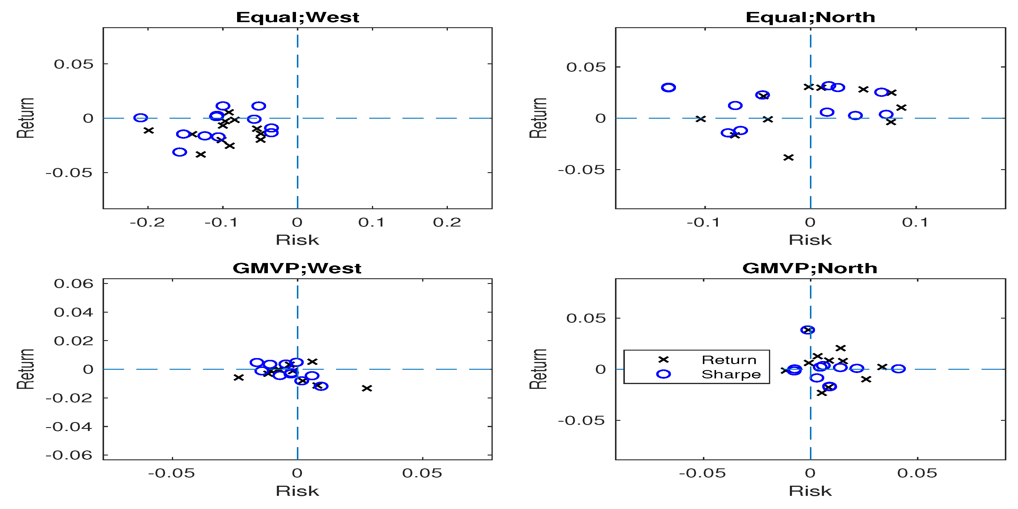
In many cases, the north portfolios are located in the north in the risk-return plane, i.e., they push the benchmark to the north by increasing mean return. For the equally-weighted portfolio and the GMVP cases, the north portfolios have higher mean return over the benchmark by and (p-value: and ) on average, respectively. In summary, when the real data were used, the west portfolios generally reduce the risk for the equally-weighted portfolio case, while the north portfolios are favorable in terms of mean return. As shown in Figure 2, the results when the 12 partially simulated datasets (dynamic setting) were considered are similar as those of the real data case.
Note that the mean returns of portfolios when 12 real datasets were considered are shown in Table 3. See Table 4 and Table 5 for the mean returns of portfolios when the dynamic and completely simulated data were considered, respectively. When the proposed portfolios have significantly (p-value ) larger mean returns than those of the benchmark, the corresponding values are marked in bold. To facilitate the presentation, the differences of mean returns of strategies are given in parenthesis in Table 3, i.e., . Here, and are mean returns of a proposed portfolio w and the benchmark v, respectively. Overall, it is seen that the north portfolios (i.e., N-R and N-S) have higher mean returns compared to the benchmark for of cases, and the improvements are significant in of cases. Among three data types, these improvements for north portfolios are not strong when the partially simulated data (dynamic components set) are considered (statistically significant in of cases). This may be due to the effect of the arbitrary initialization of for the newly added components for , when updating north selection portfolios. Future research will include comprehensive sensitivity analysis of this initialization in the dynamic setting.
To investigate whether higher returns of the north selection portfolios are not due to higher risk, the kurtosis as defined in Section 3.2 was computed. Note that kurtosis of any univariate normal distribution is 3 and higher kurtosis can be interpreted as the result of infrequent extreme outliers or deviations, unlike frequent modestly sized deviations. As reported in Table 6, Table 7 and Table 8, the west and north portfolios have kurtosis values less than 3 in of cases. This indicates that the obtained return distribution generally produces fewer and less extreme outliers than does the normal distribution, i.e., higher returns observed in the north portfolios are not due to higher risk.
4.2. Sparse, Sustainable and Stable Selection
Note that sparse, sustainable, and stable selection is crucial for investors in the portfolio selection because it is related to management and transaction costs that play a critical role in the portfolio. Recall the quantities and for the measures of sparsity and stability, respectively. Table 9, Table 10 and Table 11 record the average sparsity over times when the three data types were considered, respectively. Standard deviations of the sparsity quantities are less than for all cases. On average, the proposed portfolios generally select a few assets (less than 10%) in the considered component list.
Table 12, Table 13 and Table 14 record the average stability quantities over times. Note that standard deviations of the stability quantities are less than for all three cases. In most cases, the stability measures are less than 10%, suggesting that active assets in the are stable across times.
As shown in Table 15, the proposed portfolios’ turnovers are mostly less than . Compared to when the equally-weighted portfolio is a benchmark, the proposed portfolios when GMVP is a benchmark have generally lower turnover. This suggests that the proposed portfolios is more stable when GMVP was considered. As shown in Table 16 and Table 17, turnovers of the proposed portfolio for the dynamic setting generally larger compared to those of the static components cases.
4.3. Variance and Sharpe Ratio Comparison
The out-of-sample standard deviations and Sharpe ratio of the proposed portfolios were investigated. Table 18, Table 19 and Table 20 record the out-of-sample standard deviations and for the proposed portfolios and benchmarks, respectively, when the three data types were considered. To facilitate the presentation, the differences of standard deviations of strategies are given in parenthesis, i.e., .
For the equally-weighted portfolio case, out-of-sample standard deviations for the west portfolios are lower than those of the benchmarks, while the north portfolios generally have higher standard deviations. To test the hypothesis that the standard deviation of the returns of the benchmark v and the proposed portfolios w are equal, i.e., , the approach in DeMiguel et al. [15] and the approach presented in Remark 3.2 of Ledoit and Wolf [60] were used. When proposed portfolios have significantly lower standard deviations, the corresponding standard deviations are marked in bold in Table 18.
In about of the equally-weighted benchmark cases, the west portfolios (i.e., W-R and W-S) have significantly lower standard deviations than those of benchmark. However, when the GMVP was used as a benchmark, west portfolios usually do not improve out-of-sample standard deviations, which can be explained by the fact that GMVP is the one having the lowest in-sample standard deviations among other portfolios, thus its out-of-sample performances may also have lower values. This finding also suggests that it is essential to understand the characteristics of the benchmark when the investor construct the proposed portfolio using the benchmark. For example, it would be appropriate to apply the north selection when investor uses the GMVP as a benchmark.
Table 21, Table 22 and Table 23 record the Sharpe ratio of the proposed portfolios, when the three data types were used, respectively. To better report the differences between the performances of proposed portfolios and benchmarks, the differences of standard deviations, i.e., , in parenthesis are also recorded. The north portfolios generally have higher Sharpe ratio in most cases for the equally-weighted benchmark case, while the west portfolios generally do not improve the Sharpe ratio. The hypothesis that the Sharpe ratio of the proposed portfolio w is equivalent to that of the benchmark v () was tested. Following DeMiguel et al. [15], to obtain a two-sided p-value, the studentized circular block bootstrap [60] using 1000 bootstrap samples with a block size 5 was used.
Note that the Sharpe ratios are marked in bold in Table 21 when the proposed portfolios give a significantly higher Sharpe ratio (p-value ). For 72% of the equally-weighted benchmark cases, we see that the north portfolios give significantly higher Sharpe ratios compared to those of the corresponding benchmark portfolios, while the west portfolios improve Sharpe ratios in 52% cases. On the other hand, when the GMVP was used as a benchmark, only of the proposed portfolios are shown to significantly improve Sharpe ratios, which suggests that it is difficult to obtain significantly better risk-adjusted return than GMVP when the investor utilizes GMVP as a benchmark.
4.4. Information Ratio
Information ratio quantifies the excess return of the proposed portfolio divided by the standard deviation of the excess returns. Note that the median manager typically provides an information ratio near or below zero [61]. Table 24, Table 25 and Table 26 show the information ratio when the three data types were considered, respectively. Although west portfolios successfully reduce the risk when the investor uses the equally-weighted portfolio as a benchmark portfolio, as shown in Section 4.3, it is not favorable in terms of information ratio for many cases. On the other hand, the information ratios of the north portfolios are above zero in 83% cases and over in many cases. This suggests that the north portfolio could be favorable compared to the west portfolio in terms of Information ratio.
5. Conclusions
This paper aims to construct novel portfolios through a sparse, sustainable and stable selection from the efficient frontier. This paper proposes to hold the benchmark at certain amount α and invest in sparse and stable assets by using Dantzig-type optimization methods. Sparse, sustainable and stable asset selection is an important factor in controlling both management and transaction costs. The west selection reduces the risk compared to the benchmark, i.e., it generally pushes the benchmark to the west. The north selection pushes the benchmark to the north by increasing the expected return compared to the benchmark. In the considered 12 real datasets and their dynamic settings where the component lists are changed by time, the proposed portfolios generally select sparse, sustainable and stable assets across times. The simulation results generated by Fama–French three-factor model also shows potential advantages of the proposed models. The west selection empirically reduces the risk when the equally-weighted-portfolio is utilized as a benchmark portfolio, while the north selection could outperform the benchmark in terms of the mean return, information ratio, and Sharpe ratio. Moreover, the proposed method may enable further generalizations with a general structure of transaction costs [62]. This generalization will be considered as direction for the future work. Overall, if the investors prefer low-risk, they may take the west selection. On the other hand, if the investors expect a better return, they may take the north selection. As in Theorems 3 and 5, both the west selection and the north selection gives a stable portfolio with respect to regularization parameters as long as appropriate candidate parameters are considered. In this regard, the proposed portfolio selection could be very attractive to investors who want stable model selection with respect to change of parameters. Therefore, both the west selection and the north selection are very attractive to investors and contribute to the development of study for portfolio selection.
6. Code
The codes (MIT license) include the following steps: cleaning the data, solve the optimization problems, calculate the performance measures, and generate plots. We used MATLAB to solve the optimization problems. The codes are uploaded at https://github.com/ishspsy/project/tree/ishspsy-patch-1; “running_five_data.m” and “running_three_data.m” are the main files, and “code_graph_generate.m” reproduces all the figures in the paper.
Author Contributions
S.P. and S.L. designed the experiments; S.P. collected and analyzed the data; S.P., E.R.L., S.L. and G.K. contributed analysis tools; S.P. and E.R.L. proved the theorems in the paper; and S.P. and G.K. wrote the paper.
Funding
Seyoung Park is supported by the National Research Foundation of Korea grant funded by the Korea government (MSIP) (No. NRF-2019R1C1C1003805). Eun Ryung Lee is supported by the National Research Foundation of Korea grant funded by the Korea government (MSIT) (No. NRF-2019R1F1A1062795). Sungchul Lee is supported by the National Research Foundation of Korea grant funded by the Korea government (No. NRF-2017R1A2B2005661). Geonwoo Kim is supported by the National Research Foundation of Korea grant funded by the Korea government (No. NRF-2017R1E1A1A03070886).
Conflicts of Interest
The authors declare no conflict of interest.
Appendix A.
The proofs of main results are provided in this appendix.
Proof of Theorem 1.
Since the optimization in Equation (4) includes an additional constraint (related to return) to the optimization in Equation (3), it is enough to prove that Equation (4) is a semidefinite programming problem. Equation (4) can be rewritten as
which is equivalent to the following semidefinite programming problem:
where is the p by p diagonal matrix whose diagonal components are , and means that X is positive semidefinite. By using the fact that
when A and C are square matrices and C is invertible, the constraint in Equation (A1) implies . This completes the proof. □
To prove the rest of theorems, the Lagrangian expression of the proposed optimizations should be developed first. By the Lagrange multiplier method, the west selection problem in Equation (3) is to minimize
Let be the sub-gradient vector of , i.e., the ith element of g is
Then, the Karush–Kuhn–Tucker (KKT) optimality conditions are
By using the same argument, the KKT optimality conditions of the north selection problem in Equation (4) are
Appendix A.1. Proof of Theorem 2
Proof.
By the Lagrange multiplier method, the optimization problem in Theorem 2 is to minimize
where is the Lagrange multiplier. Then, the Karush–Kuhn–Tucker (KKT) optimality conditions are
Since , , are the solutions to Equation (A2) and g is the sub-gradient evaluated at , we have with
where . Therefore, the solution to Equation (3) is also the solution to the optimization problem in Theorem 2. This completes the proof. □
Appendix A.2. Proof of Theorem 3
Proof.
First, consider the case that the risk constraint of is unbinding, i.e., . Let be the west selection portfolio with , i.e., no risk constraint case. Suppose that . Since the risk constraint is a convex, there exists a such that and . Since , it holds that
which contradicts the fact that is a solution to Equation (3) with a parameter . Hence, , i.e., . This means that for any , i.e., and .
Second, consider the case that the risk constraint of is binding, i.e., . Hence, it holds that
which implies , i.e., . By letting be the minimum eigenvalue of , it holds that . This completes the proof. □
Appendix A.3. Proof of Theorem 4
Since the proof is essentially the same as that of Theorem 2, the proof is omitted.
Appendix A.4. Proof of Theorem 5
Proof.
First, consider the case that the return constraint of is unbinding, i.e., . Suppose that . Since the return constraint is convex, there exists some constant such that and . Since , it holds that
which contradicts the fact that is a solution to Equation (4) with a parameter . Hence, , i.e., . This means that for any , i.e., and .
Second, consider the case that the return constraint of is binding, i.e., . Hence, it holds that
This completes the proof. □
References
- Markowitz, H.M. Portfolio selection. J. Finance 1952, 7, 77–91. [Google Scholar]
- Best, M.J.; Grauer, R.R. On the sensitivity of mean-variance-efficient portfolios to changes in asset means: some analytical and computational results. Rev. Financ. Stud. 1991, 4, 315–342. [Google Scholar]
- Chopra, V.K.; Ziemba, W.T. The effect of errors in means, variances, and covariances on optimal portfolio choice. J. Portf. Manag. 1993, 19, 6–11. [Google Scholar]
- Merton, R.C. On estimating the expected return on the market: An exploratory investigation. J. Financ. Econ. 1980, 8, 323–361. [Google Scholar]
- DeMiguel, V.; Garlappi, L.; Uppal, R. Optimal versus naive diversification: How inefficient is the 1/n portfolio strategy? Rev. Financ. Stud. 2009, 22, 1915–1953. [Google Scholar]
- Michaud, R.O. The Markowitz optimization enigma: Is optimized optimal? Financ. Anal. J. 1989, 45, 31–42. [Google Scholar]
- Green, R.; Hollifield, B. When will mean-variance efficient portfolios be well diversified? J. Finance 1992, 47, 1785–1809. [Google Scholar]
- Chan, L.K.C.; Karceski, J.; Lakonishok, J. On portfolio optimization: Forecasting covariances and choosing the risk model. Rev. Financ. Stud. 1999, 12, 937–974. [Google Scholar]
- Carvalho, C.M.; West, M. Dynamic matrix-variate graphical models. Bayesian Anal. 2007, 2, 69–98. [Google Scholar]
- Jagannathan, R.; Ma, T. Risk reduction in large portfolios: Why imposing the wrong constraints helps. J. Financ. 2003, 58, 1651–1683. [Google Scholar]
- Ledoit, O.; Wolf, M. Honey, I shrunk the sample covariance matrix. J. Portf. Manag. 2004, 30, 110–119. [Google Scholar]
- Frost, P.A.; Savarino, J.E. For better performance constrain portfolio weights. J. Portf. Manag. 1988, 15, 29–34. [Google Scholar]
- Chopra, V.K. Improving optimization. J. Investig. 1993, 8, 51–59. [Google Scholar]
- Lobo, M.S.; Fazel, M.; Boyd, S. Portfolio optimization with linear and fixed transaction costs. Annal. Operat. Res. 2007, 152, 341–365. [Google Scholar]
- DeMiguel, V.; Garlappi, L.; Nogales, F.; Uppal, R. A generalized approach to portfolio optimization: Improving performance by constraining portfolio norms. Manag. Sci. 2009, 55, 798–812. [Google Scholar]
- Brodie, J.; Daubechies, I.; De Mol, C.; Giannone, D.; Loris, I. Sparse and stable Markowitz portfolios. Proc. Natl. Acad. Sci. USA 2009, 106, 12267–12272. [Google Scholar] [Green Version]
- Fan, J.; Zhang, J.; Yu, K. Vast portfolio selection with gross-exposure constraints. JASA 2012, 107, 592–606. [Google Scholar]
- Xing, X.; Hu, J.; Yang, Y. Robust minimum variance portfolio with L-infinity constraints. J. Bank. Financ. 2014, 46, 107–117. [Google Scholar]
- Park, S.; Song, H.; Lee, S. Linear programing models for portfolio optimization using a benchmark. Eur. J. Financ. 2019, 25, 435–457. [Google Scholar]
- Zhang, Y.; Liu, Z.; Yu, X. The Diversification Benefits of Including Carbon Assets in Financial Portfolios. Sustainability 2017, 9, 437. [Google Scholar] [Green Version]
- Li, Z.; Li, X.; Hui, Y.; Wong, W.K. Maslow Portfolio Selection for Individuals with Low Financial Sustainability. Sustainability 2018, 10, 1128. [Google Scholar] [Green Version]
- Raudys, S.; Raudys, A.; Pabarskaite, Z. Dynamically Controlled Length of Training Data for Sustainable Portfolio Selection. Sustainability 2018, 10, 1911. [Google Scholar] [Green Version]
- Joyo, A.S.; Lefen, L. Stock Market Integration of Pakistan with Its Trading Partners: A Multivariate DCC-GARCH Model Approach. Sustainability 2019, 11, 303. [Google Scholar] [Green Version]
- Roll, R. A mean/variance analysis of tracking error. J. Portf. Manag. 1992, 18, 13–22. [Google Scholar]
- Jorion, P. Portfolio optimization with tracking-error constraints. Financ. Anal. J. 2003, 59, 70–82. [Google Scholar]
- Shen, W.; Wang, J.; Ma, S. Doubly regularized portfolio with risk minimization. In Proceedings of the Twenty-Eighth AAAI Conference on Artificial Intelligence, Québec City, QC, Canada, 27–31 July 2014; pp. 1286–1292. [Google Scholar]
- Kopa, M.; Post, T. A general test for ssd portfolio efficiency. OR Spectr. 2014, 37, 703–734. [Google Scholar]
- Hodder, J.E.; Jackwerth, J.C.; Kolokolova, O. Improved portfolio choice using second-order stochastic dominance. Rev. Financ. 2015, 19, 1623–1647. [Google Scholar]
- Kuosmanen, T. Efficient diversification according to stochastic dominance criteria. Manag. Sci. 2004, 50, 1390–1406. [Google Scholar]
- Luedtke, J. New formulations for optimization under stochastic dominance constraints. SIAM J. Optim. 2008, 19, 1433–1450. [Google Scholar]
- Bruni, R.; Cesarone, F.; Scozzari, A.; Tardella, F. A linear risk-return model for enhanced indexation in portfolio optimization. OR Spectr. 2017, 37, 735–759. [Google Scholar]
- Fábián, C.I.; Mitra, G.; Roman, D.; Zverovich, V. An enhanced model for portfolio choice with ssd criteria: A constructive approach. Quant. Financ. 2011, 11, 1525–1534. [Google Scholar]
- Guastaroba, G.; Speranza, M.G. Kernel search: An application to the index tracking problem. Eur. J. Operat. Res. 2012, 217, 54–68. [Google Scholar]
- Levy, H. Stochastic dominance and expected utility: Survey and analysis. Manag. Sci. 1992, 38, 555–593. [Google Scholar]
- Levy, H. Stochastic Dominance: Investment Decision Making under Uncertainty, 2nd ed.; Springer: New York, NY, USA, 2016. [Google Scholar]
- Sarker, B.; Jamal, A.A.M.; Mondal, S. Optimal batch sizing in a multi-stage production system with rework consideration. Eur. J. Oper. Res. 2008, 184, 915–929. [Google Scholar]
- Kim, M.; Sarkar, B. Multi-stage cleaner production process with quality improvement and lead time dependent ordering cost. J. Clean. Prod. 2019, 144, 572–590. [Google Scholar]
- Tayyab, M.; Sarkar, B. Optimal batch quantity in a cleaner multi-stage lean production system with random defective rate. J. Clean. Prod. 2016, 139, 922–934. [Google Scholar]
- Sarkar, B. Mathematical and analytical approach for the management of defective items in a multi-stage production system. J. Clean. Prod. 2019, 218, 896–919. [Google Scholar]
- Tibshirani, R. Regression shrinkage and selection via the Lasso. J. Roy. Statist. Soc. Ser. B 1996, 58, 267–288. [Google Scholar]
- Ruiz-Torrubiano, R.; Suárez, A. A hybrid optimization approach to index tracking. Ann. Oper. Res. 2009, 166, 57–71. [Google Scholar]
- Gilli, M.; Kellezi, E. The threshold accepting heuristic for index tracking. Financial Engineering, E-Commerce, and Supply Chain. Kluwer Appl. Optim. Ser. 2002, 70, 1–18. [Google Scholar]
- Beasley, J.E.; Meade, N.; Chang, T.J. An evolutionary heuristic for the index tracking problem. Eur. J. Operat. Res. 2003, 148, 621–643. [Google Scholar]
- Ni, H.; Wang, Y. Stock index tracking by pareto efficient genetic algorithm. Appl. Soft Comput. 2013, 13, 4519–4535. [Google Scholar]
- Zou, H. The adaptive Lasso and its oracle properties. JASA 2006, 10, 1418–1429. [Google Scholar]
- Zou, H.; Zhang, H.H. On the adaptive elastic-net with a diverging number of parameters. Ann. Stat. 2009, 37, 1733–1751. [Google Scholar] [Green Version]
- Chatterjee, A.; Lahiri, S.N. Rates of convergence of the adaptive lasso estimators to the oracle distribution and higher order refinements by the bootstrap. Ann. Stat. 2013, 41, 1232–1259. [Google Scholar]
- Candes, E.; Tao, T. The Dantzig selector: Statistical estimation when p is much larger than n. Ann. Stat. 2007, 35, 2313–2351. [Google Scholar]
- Park, S.; He, X.; Zhou, S. Dantzig-type penalization for multiple quantile regression with high dimensional covariates. Stat. Sin. 2017, 27, 1619–1638. [Google Scholar]
- Toh, K.C.; Todd, M.J.; Tütüncü, R.H. On the Implementation and Usage of SDPT3–A Matlab Software Package for Semidefinite-Quadratic-Linear Programming, Version 4.0. Handbook on Semidefinite, Conic and Polynomial Optimization. Int. Ser. Operat. Res. Manag. Sci. 2012, 166, 715–754. [Google Scholar]
- Ledoit, O.; Wolf, M. Improved estimation of the covariance matrix of stock returns with an application to portfolio selection. J. Empir. Financ. 2003, 10, 603–621. [Google Scholar]
- Alexander, C. Market Models: A Guide to Financial Data Analysis; Wiley: Hoboken, NJ, USA, 2001. [Google Scholar]
- Engle, R.F. Autoregressive conditional heteroscedasticity with estimates of the variance of united kingdom inflation. Econometrica 1982, 50, 987–1007. [Google Scholar]
- Bollerslev, T. Generalized autoregressive conditional heteroskedasticity. J. Econom. 1986, 31, 307–327. [Google Scholar] [Green Version]
- Fan, J. High dimensional covariance matrix estimation using a factor model. J. Econom. 2008, 147, 186–197. [Google Scholar] [Green Version]
- Bai, J.; Li, K. Statistical analysis of factor models of high dimension. Ann. Stat. 2012, 40, 436–465. [Google Scholar] [Green Version]
- Fan, J.; Liao, Y.; Mincheva, M. Large covariance estimation by thresholding principal orthogonal complements. J. Roy. Statist. Soc. Ser. B 2013, 75, 603–680. [Google Scholar] [Green Version]
- Fama, E.; French, K. Common risk factors in the returns on stocks and bonds. J. Financ. Econ. 1993, 33, 3–56. [Google Scholar]
- Bruni, R.; Cesarone, F.; Scozzari, A.; Tardella, F. Common risk factors in the returns on stocks and bonds. Eur. J. Oper. Res. 2017, 259, 322–329. [Google Scholar]
- Ledoit, O.; Wolf, M. Robust performance hypothesis testing with the sharpe ratio. J. Empir. Financ. 2008, 15, 850–859. [Google Scholar]
- Grinold, R.C.; Kahn, R.N. Active Portfolio Management; McGraw-Hill: New York, NY, USA, 2000. [Google Scholar]
- Beraldi, P.; Violi, A.; Ferrara, M.; Ciancio, C.; Pansera, B.A. Dealing with complex transaction costs in portfolio management. In Annals of Operations Research; Springer: Berlin, Germany, 2019. [Google Scholar]
Figure 1.
Positions of the proposed portfolios based on the benchmark portfolio when 12 real datasets were used. The circle and cross points indicate the portfolios using Sharpe ratio and mean return as criterion functions, respectively. As the 12 datasets are considered for the equally-weighted and GMVP portfolios, each subplot consists of points.
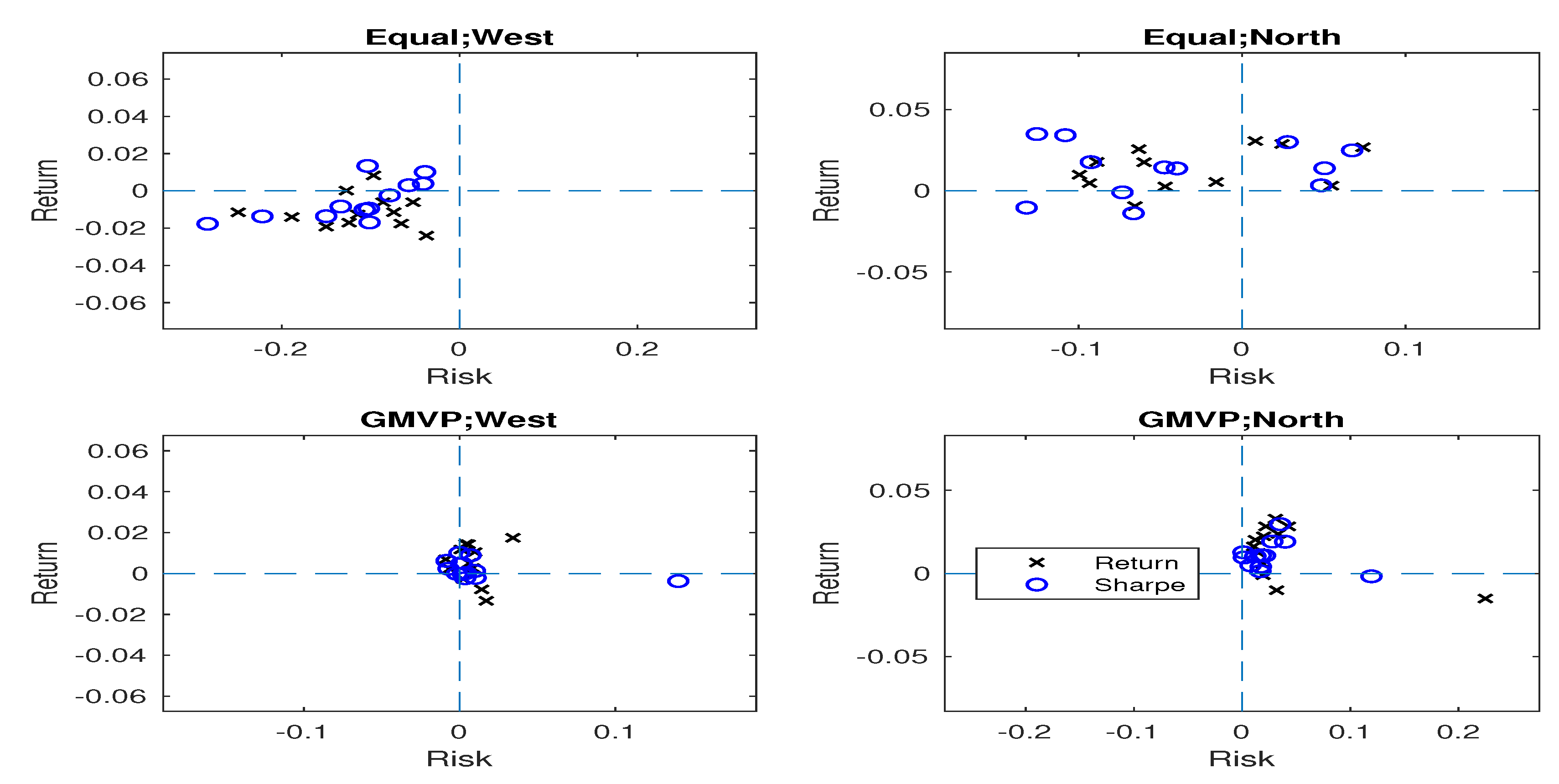
Figure 2.
Positions of the proposed portfolios based on the benchmark portfolio when the partially simulated data were considered. The circle and cross points indicate the portfolios using Sharpe ratio and mean return as criterion functions, respectively. As the 12 datasets are considered for the equally-weighted and GMVP portfolios, each subplot consists of points.


Table 1.
Comparison between contributions of different authors in terms of optimization, parameter selection, and performance measures.
Table 1.
Comparison between contributions of different authors in terms of optimization, parameter selection, and performance measures.
| Method | Optimization | Parameter Selection | Performances | |||||||
|---|---|---|---|---|---|---|---|---|---|---|
| Return | Risk | Sparsity | Stability | Cross-validation | Fixed | Return | Skewness | Turnovers | Sharpe Ratio | |
| Proposed west selection | ✓ | ✓ | ✓ | ✓ | ✓ | ✓ | ✓ | ✓ | ||
| Proposed north selection | ✓ | ✓ | ✓ | ✓ | ✓ | ✓ | ✓ | ✓ | ✓ | |
| Lobo et al. [14] | ✓ | ✓ | ✓ | ✓ | ✓ | |||||
| DeMiguel et al. [15] | ✓ | ✓ | ✓ | ✓ | ✓ | |||||
| Brodie et al. [16] | ✓ | ✓ | ✓ | ✓ | ✓ | ✓ | ||||
| Xing et al. [18] | ✓ | ✓ | ✓ | ✓ | ✓ | ✓ | ✓ | |||
| Roll [24] | ✓ | ✓ | ✓ | ✓ | ||||||
| Jorion [25] | ✓ | ✓ | ✓ | ✓ | ✓ | |||||
| Shen et al. [26] | ✓ | ✓ | ✓ | ✓ | ✓ | ✓ | ✓ | |||
| Ruiz-Torrubiano and Suárez [41] | ✓ | ✓ | ✓ | ✓ | ||||||
| Gilli and Kellezi [42] | ✓ | ✓ | ✓ | ✓ | ✓ | ✓ | ||||
| Beasley et al. [43] | ✓ | ✓ | ✓ | ✓ | ||||||
| Ni and Wang [44] | ✓ | ✓ | ✓ | ✓ | ✓ | |||||
| Hodder, Jackwerth, and Kolokolova [28] | ✓ | ✓ | ✓ | ✓ | ✓ | ✓ | ✓ | |||
| Kuosmanen [29] | ✓ | ✓ | ✓ | ✓ | ✓ | ✓ | ✓ | |||
| Luedtke [30] | ✓ | ✓ | ✓ | ✓ | ✓ | ✓ | ||||
| Bruni et al. [31] | ✓ | ✓ | ✓ | ✓ | ✓ | ✓ | ||||
| Fábián et al. [32] | ✓ | ✓ | ✓ | ✓ | ✓ | ✓ | ||||
| Guastaroba and Speranza [33] | ✓ | ✓ | ✓ | ✓ | ✓ | |||||
Table 2.
Portfolio selection methods, cross-validation performance measures, and abbreviations.
| Method | Cross-Validation Criterion | Abbreviation |
|---|---|---|
| West selection | Mean return | W-R |
| Sharpe ratio | W-S | |
| North selection | Mean return | N-R |
| Sharpe ratio | N-S |
Table 3.
Average monthly returns of the proposed portfolios and benchmark for the 12 real datasets case. The two benchmark portfolios, equally-weighted portfolio and GMVP, were considered when constructing the portfolios, respectively. The differences of mean returns between proposed portfolios and benchmark are also given in parenthesis. “Bench” represents the benchmark, and “W-R” (“N-R”) and “W-S” (“N-S”) represent the west (north) portfolios using the mean return and Sharpe ratio as criterion functions in the cross validation, respectively.
| Data | Equally-Weighted | GMVP | ||||||||
|---|---|---|---|---|---|---|---|---|---|---|
| Bench | W-R | W-S | N-R | N-S | Bench | W-R | W-S | N-R | N-S | |
| DOW30 | 0.129 | 0.114 | 0.110 | 0.149 | 0.138 | 0.107 | 0.102 | 0.105 | 0.107 | 0.113 |
| (−0.015) | (−0.019) | (0.020) | (0.009) | (−0.005) | (−0.002) | (0.000) | (0.006) | |||
| DAX30 | 0.117 | 0.098 | 0.106 | 0.122 | 0.120 | 0.101 | 0.105 | 0.105 | 0.108 | 0.115 |
| (−0.019) | (−0.011) | (0.005) | (0.003) | (0.004) | (0.004) | (0.007) | (0.014) | |||
| FTSE100 | 0.135 | 0.134 | 0.123 | 0.159 | 0.160 | 0.125 | 0.133 | 0.132 | 0.144 | 0.151 |
| (−0.001) | (−0.012) | (0.024) | (0.025) | (0.008) | (0.007) | (0.019) | (0.026) | |||
| SP100 | 0.128 | 0.120 | 0.136 | 0.133 | 0.158 | 0.112 | 0.112 | 0.111 | 0.127 | 0.117 |
| (−0.008) | (0.008) | (0.005) | (0.030) | (0.000) | (−0.001) | (0.015) | (0.005) | |||
| FTSE250 | 0.145 | 0.119 | 0.146 | 0.147 | 0.149 | 0.158 | 0.143 | 0.154 | 0.143 | 0.157 |
| (−0.026) | (0.001) | (0.002) | (0.004) | (−0.015) | (−0.004) | (−0.015) | (−0.001) | |||
| SP500 | 0.143 | 0.130 | 0.144 | 0.143 | 0.172 | 0.074 | 0.077 | 0.072 | 0.097 | 0.073 |
| (−0.013) | (0.001) | (0.001) | (0.029) | (0.003) | (−0.002) | (0.023) | (−0.001) | |||
| Hang Seng | 0.038 | 0.022 | 0.022 | 0.059 | 0.057 | 0.060 | 0.061 | 0.061 | 0.088 | 0.066 |
| (−0.016) | (−0.016) | (0.021) | (0.019) | (0.001) | (0.001) | (0.028) | (0.006) | |||
| FF49 | 0.118 | 0.125 | 0.130 | 0.131 | 0.131 | 0.109 | 0.109 | 0.103 | 0.110 | 0.111 |
| (0.007) | (0.012) | (0.013) | (0.013) | (0.001) | (−0.006) | (0.001) | (0.002) | |||
| NASDAQ100 | 0.170 | 0.151 | 0.159 | 0.196 | 0.179 | 0.113 | 0.129 | 0.109 | 0.136 | 0.127 |
| (−0.019) | (−0.011) | (0.026) | (0.009) | (0.016) | (−0.004) | (0.023) | (0.014) | |||
| Euro Stoxx50 | 0.093 | 0.085 | 0.088 | 0.091 | 0.093 | 0.101 | 0.111 | 0.099 | 0.103 | 0.102 |
| (−0.008) | (−0.005) | (−0.002) | (0.000) | (0.010) | (−0.002) | (0.002) | (0.001) | |||
| NASDAQ3000 | 0.149 | 0.128 | 0.133 | 0.161 | 0.158 | 0.077 | 0.089 | 0.080 | 0.094 | 0.081 |
| (−0.021) | (−0.016) | (0.012) | (0.009) | (0.012) | (0.003) | (0.017) | (0.004) | |||
| RUSSELL2000 | 0.146 | 0.133 | 0.127 | 0.147 | 0.131 | 0.060 | 0.073 | 0.068 | 0.072 | 0.068 |
| (−0.013) | (−0.019) | (0.001) | (−0.015) | (0.013) | (0.008) | (0.012) | (0.008) | |||
Table 4.
Average monthly returns of the proposed portfolios and benchmark when partially simulated data were considered.
Table 4.
Average monthly returns of the proposed portfolios and benchmark when partially simulated data were considered.
| Data | Equally-Weighted | GMVP | ||||||||
|---|---|---|---|---|---|---|---|---|---|---|
| Bench | W-R | W-S | N-R | N-S | Bench | W-R | W-S | N-R | N-S | |
| DOW30 | 0.127 | 0.107 | 0.111 | 0.157 | 0.158 | 0.102 | 0.100 | 0.099 | 0.110 | 0.104 |
| (−0.020) | (−0.016) | (0.030) | (0.031) | (−0.002 ) | (−0.003) | (0.008) | (0.002) | |||
| DAX30 | 0.113 | 0.098 | 0.098 | 0.096 | 0.101 | 0.094 | 0.086 | 0.086 | 0.102 | 0.096 |
| (−0.015) | (−0.015) | (−0.017) | (−0.012) | (−0.008) | (−0.008) | (0.008) | (0.002) | |||
| FTSE100 | 0.127 | 0.124 | 0.128 | 0.155 | 0.157 | 0.133 | 0.136 | 0.137 | 0.145 | 0.136 |
| (−0.003) | (0.001) | (0.028) | (0.030) | (0.003) | (0.004) | (0.012) | (0.003) | |||
| SP100 | 0.125 | 0.111 | 0.116 | 0.124 | 0.155 | 0.109 | 0.114 | 0.106 | 0.115 | 0.101 |
| (−0.014) | (−0.009) | (−0.001) | (0.030) | (0.005) | (−0.003) | (0.006) | (−0.008) | |||
| FTSE250 | 0.137 | 0.127 | 0.136 | 0.136 | 0.149 | 0.144 | 0.131 | 0.140 | 0.135 | 0.145 |
| (−0.010) | (−0.001) | (−0.001) | (0.012) | (−0.013) | (−0.004) | (−0.009) | (0.001) | |||
| SP500 | 0.125 | 0.105 | 0.112 | 0.124 | 0.155 | 0.109 | 0.114 | 0.106 | 0.115 | 0.101 |
| (−0.020) | (−0.013) | (−0.001) | (0.030) | (0.005) | (−0.003) | (0.006) | (−0.008) | |||
| Hang Seng | 0.026 | 0.015 | 0.026 | 0.051 | 0.051 | 0.076 | 0.065 | 0.065 | 0.097 | 0.077 |
| (−0.011) | (0.000) | (0.025) | (0.025) | (−0.011) | (−0.011) | (0.021) | (0.001) | |||
| FF49 | 0.095 | 0.101 | 0.107 | 0.117 | 0.118 | 0.708 | 0.698 | 0.697 | 1.092 | 1.092 |
| (0.006) | (0.012) | (0.022) | (0.023) | (−0.010) | (−0.011) | (0.384) | (0.384) | |||
| NASDAQ100 | 0.164 | 0.139 | 0.147 | 0.194 | 0.170 | 0.130 | 0.127 | 0.134 | 0.107 | 0.130 |
| (−0.025) | (−0.017) | (0.030) | (0.006) | (−0.003) | (0.004) | (−0.023) | (0.000) | |||
| Euro Stoxx50 | 0.089 | 0.087 | 0.100 | 0.085 | 0.091 | 0.105 | 0.105 | 0.101 | 0.104 | 0.104 |
| (−0.002) | (0.011) | (−0.004) | (0.002) | (0.000) | (−0.004) | (−0.001) | (−0.001) | |||
| NASDAQ3000 | 0.191 | 0.184 | 0.193 | 0.201 | 0.195 | 0.157 | 0.157 | 0.161 | 0.159 | 0.140 |
| (−0.007) | (0.002) | (0.010) | (0.004) | (0.000) | (0.004) | (0.002) | (−0.017) | |||
| RUSSELL2000 | 0.174 | 0.140 | 0.143 | 0.136 | 0.160 | 0.159 | 0.153 | 0.162 | 0.141 | 0.142 |
| (−0.034) | (−0.031) | (−0.038) | (−0.014) | (−0.006) | (0.003) | (−0.018) | (−0.017) | |||
Table 5.
Average monthly returns of the proposed portfolios and benchmark over six different evaluation periods when completely simulated data were considered. The two benchmark portfolios, equally-weighted portfolio and GMVP, were considered when constructing the proposed portfolios, respectively, and was used in simulation, where p represents the number of static components in the simulation model.
| Case | Evaluation Period | Equally-Weighted | GMVP | ||||||||
|---|---|---|---|---|---|---|---|---|---|---|---|
| Bench | W-R | W-S | N-R | N-S | Bench | W-R | W-S | N-R | N-S | ||
| 1–5000 | 0.597 | 0.603 | 0.533 | 0.674 | 0.653 | 0.002 | 0.033 | 0.024 | 0.043 | 0.036 | |
| (0.006) | (−0.064) | (0.077) | (0.056) | (0.031) | (0.022) | (0.041) | (0.034) | ||||
| 1–1000 | 0.027 | 0.089 | 0.084 | 0.060 | 0.092 | −0.002 | −0.006 | 0.016 | 0.006 | 0.014 | |
| (0.062) | (0.057) | (0.033) | (0.065) | (−0.004) | (0.018) | (0.008) | (0.016) | ||||
| 1001–2000 | −0.508 | −0.287 | −0.360 | −0.242 | −0.395 | −0.002 | −0.005 | −0.003 | 0.009 | 0.017 | |
| (0.221) | (0.148) | (0.266) | (0.113) | (−0.003) | (−0.001) | (0.011) | (0.019) | ||||
| 2001–3000 | 1.219 | 1.057 | 0.943 | 1.108 | 1.122 | 0.006 | 0.055 | 0.022 | 0.063 | 0.047 | |
| (−0.162) | (−0.276) | (−0.111) | (−0.097) | (0.049) | (0.016) | (0.057) | (0.041) | ||||
| 3001–4000 | 1.482 | 1.385 | 1.259 | 1.443 | 1.448 | 0.007 | 0.072 | 0.045 | 0.076 | 0.056 | |
| (−0.097) | (−0.223) | (−0.039) | (−0.034) | (0.065) | (0.038) | (0.069) | (0.049) | ||||
| 4001–5000 | 0.752 | 0.757 | 0.720 | 0.971 | 0.967 | 0.003 | 0.049 | 0.037 | 0.058 | 0.045 | |
| (0.005) | (−0.032) | (0.219) | (0.215) | (0.046) | (0.034) | (0.055) | (0.042) | ||||
| 1–5000 | 0.497 | 0.558 | 0.540 | 0.542 | 0.574 | 0.001 | 0.030 | 0.013 | 0.032 | 0.016 | |
| (0.061) | (0.043) | (0.045) | (0.077) | (0.029) | (0.012) | (0.031) | (0.015) | ||||
| 1–1000 | −0.972 | −0.710 | −0.696 | −0.937 | −0.896 | −0.001 | −0.007 | −0.012 | −0.016 | −0.021 | |
| (0.262) | (0.276) | (0.035) | (0.076) | (−0.006) | (−0.011) | (−0.015) | (−0.020) | ||||
| 1001–2000 | 0.364 | 0.429 | 0.443 | 0.400 | 0.455 | 0.001 | −0.003 | 0.011 | 0.015 | 0.016 | |
| (0.065) | (0.079) | (0.036) | (0.091) | (−0.004) | (0.010) | (0.014) | (0.015) | ||||
| 2001–3000 | 1.541 | 1.527 | 1.369 | 1.502 | 1.556 | 0.002 | 0.068 | 0.034 | 0.070 | 0.042 | |
| (−0.014) | (−0.172) | (−0.039) | (0.015) | (0.066) | (0.032) | (0.068) | (0.040) | ||||
| 3001–4000 | 1.420 | 1.346 | 1.225 | 1.529 | 1.509 | 0.002 | 0.083 | 0.029 | 0.081 | 0.030 | |
| (−0.074) | (−0.195) | (0.109) | (0.089) | (0.081) | (0.027) | (0.079) | (0.028) | ||||
| 4001–5000 | 0.166 | 0.230 | 0.375 | 0.242 | 0.276 | 0.001 | 0.011 | 0.005 | 0.010 | 0.014 | |
| (0.064) | (0.209) | (0.076) | (0.110) | (0.010) | (0.004) | (0.009) | (0.013) | ||||
Table 6.
Kurtosis of the proposed portfolio when 12 real datasets were considered. The two benchmark portfolios, equally-weighted portfolio and GMVP, were considered when constructing the proposed portfolios, respectively. Kurtosis of any univariate normal distribution is 3. A higher kurtosis indicates infrequent extreme outliers or deviations in returns. “W-R” (“N-R”) and “W-S” (“N-S”) represent the west (north) portfolios using the mean return and Sharpe ratio as criterion functions in the cross validation, respectively.
| Data | Equally-Weighted | GMVP | ||||||
|---|---|---|---|---|---|---|---|---|
| W-R | W-S | N-R | N-S | W-R | W-S | N-R | N-S | |
| DOW30 | 2.55 | 2.61 | 2.49 | 2.50 | 1.99 | 1.99 | 2.01 | 1.93 |
| DAX30 | 2.57 | 2.51 | 2.30 | 2.24 | 2.87 | 2.97 | 2.91 | 2.88 |
| FTSE100 | 2.95 | 2.96 | 2.77 | 2.76 | 2.46 | 2.40 | 2.43 | 2.40 |
| SP100 | 2.46 | 2.29 | 2.30 | 2.20 | 2.31 | 2.29 | 2.03 | 2.16 |
| FTSE250 | 3.03 | 2.88 | 3.05 | 2.99 | 2.05 | 2.10 | 2.46 | 2.13 |
| SP500 | 2.18 | 2.38 | 2.25 | 2.20 | 2.51 | 2.24 | 2.10 | 2.12 |
| Hang Seng | 2.43 | 2.46 | 2.45 | 2.33 | 2.48 | 2.42 | 2.16 | 2.31 |
| FF49 | 2.66 | 2.82 | 2.99 | 3.09 | 2.25 | 2.29 | 2.19 | 2.32 |
| NASDAQ100 | 2.51 | 2.30 | 2.68 | 2.66 | 2.32 | 2.39 | 2.40 | 2.46 |
| Euro Stoxx50 | 2.52 | 2.64 | 2.57 | 2.59 | 2.22 | 2.38 | 2.35 | 2.38 |
| NASDAQ3000 | 1.93 | 2.32 | 2.20 | 1.98 | 1.93 | 2.32 | 2.20 | 1.98 |
| RUSSELL2000 | 2.45 | 2.29 | 1.97 | 1.93 | 2.45 | 2.29 | 1.97 | 1.93 |
Table 7.
Kurtosis of the proposed portfolio when partially simulated data were considered.
| Data | Equally-Weighted | GMVP | ||||||
|---|---|---|---|---|---|---|---|---|
| W-R | W-S | N-R | N-S | W-R | W-S | N-R | N-S | |
| DOW30 | 2.47 | 2.53 | 2.56 | 2.57 | 2.03 | 2.01 | 2.01 | 2.02 |
| DAX30 | 2.58 | 2.49 | 2.18 | 2.24 | 3.33 | 3.32 | 3.06 | 2.97 |
| FTSE100 | 2.90 | 2.99 | 2.81 | 2.91 | 2.57 | 2.30 | 2.34 | 2.39 |
| SP100 | 2.52 | 2.54 | 2.44 | 2.18 | 2.33 | 2.29 | 2.23 | 2.17 |
| FTSE250 | 3.07 | 3.13 | 2.74 | 3.01 | 2.19 | 2.22 | 2.34 | 2.21 |
| SP500 | 2.46 | 2.46 | 2.44 | 2.18 | 2.33 | 2.29 | 2.23 | 2.17 |
| Hang Seng | 2.47 | 2.46 | 2.34 | 2.31 | 2.81 | 2.79 | 2.48 | 2.51 |
| FF49 | 2.81 | 2.67 | 2.73 | 2.75 | 2.70 | 2.76 | 2.65 | 2.68 |
| NASDAQ100 | 2.38 | 2.35 | 2.69 | 2.72 | 2.41 | 2.25 | 2.41 | 2.22 |
| Euro Stoxx50 | 2.40 | 2.43 | 2.41 | 2.33 | 2.22 | 2.25 | 2.34 | 2.20 |
| NASDAQ3000 | 2.16 | 2.05 | 1.94 | 1.99 | 2.17 | 2.19 | 2.38 | 2.23 |
| RUSSELL2000 | 2.09 | 2.21 | 1.98 | 2.06 | 2.38 | 2.39 | 2.24 | 2.20 |
Table 8.
Kurtosis of the proposed portfolio over six different evaluation periods when completely simulated data were considered.
Table 8.
Kurtosis of the proposed portfolio over six different evaluation periods when completely simulated data were considered.
| Case | Evaluation Period (T) | Equally-Weighted | GMVP | ||||||
|---|---|---|---|---|---|---|---|---|---|
| W-R | W-S | N-R | N-S | W-R | W-S | N-R | N-S | ||
| 1–5000 | 2.91 | 2.76 | 2.91 | 2.83 | 3.05 | 2.85 | 3.50 | 3.21 | |
| 1–1000 | 2.11 | 2.29 | 2.19 | 2.27 | 3.34 | 2.87 | 2.90 | 2.56 | |
| 1001–2000 | 2.13 | 2.31 | 2.82 | 2.68 | 3.56 | 3.50 | 3.12 | 3.33 | |
| 2001–3000 | 2.14 | 2.11 | 1.91 | 1.93 | 2.07 | 2.80 | 2.07 | 1.96 | |
| 3001–4000 | 3.24 | 3.14 | 2.92 | 2.83 | 3.03 | 3.65 | 2.78 | 2.74 | |
| 4001–5000 | 2.82 | 2.53 | 2.86 | 2.83 | 3.66 | 3.55 | 3.29 | 3.39 | |
| 1–5000 | 2.89 | 2.85 | 2.81 | 2.82 | 3.95 | 3.72 | 3.60 | 3.09 | |
| 1–1000 | 1.91 | 1.89 | 1.89 | 1.90 | 2.34 | 2.98 | 3.30 | 3.66 | |
| 1001–2000 | 2.57 | 2.57 | 2.79 | 2.84 | 3.48 | 2.90 | 3.01 | 2.97 | |
| 2001–3000 | 2.66 | 2.49 | 2.54 | 2.64 | 3.40 | 3.24 | 3.18 | 3.56 | |
| 3001–4000 | 2.48 | 2.88 | 2.54 | 2.55 | 2.53 | 3.58 | 2.59 | 3.51 | |
| 4001–5000 | 2.83 | 2.73 | 2.52 | 2.55 | 3.01 | 2.94 | 2.78 | 3.30 | |
Table 9.
Sparsity of the proposed portfolios and benchmark portfolios when 12 real datasets were used. Two benchmark portfolios, equally-weighted portfolio and GMVP, were considered when constructing the proposed portfolios, respectively. “Bench” represents the benchmark, and “W-R” (“N-R”) and “W-S” (“N-S”) represent the west (north) portfolios using the mean return and Sharpe ratio as criterion functions in the cross validation, respectively.
| Data | Equally-Weighted | GMVP | ||||||
|---|---|---|---|---|---|---|---|---|
| W-R | W-S | N-R | N-S | W-R | W-S | N-R | N-S | |
| DOW30 | 0.05 | 0.05 | 0.08 | 0.08 | 0.03 | 0.03 | 0.06 | 0.05 |
| DAX30 | 0.06 | 0.07 | 0.08 | 0.08 | 0.04 | 0.04 | 0.07 | 0.06 |
| FTSE100 | 0.02 | 0.03 | 0.03 | 0.03 | 0.01 | 0.01 | 0.02 | 0.03 |
| SP100 | 0.02 | 0.02 | 0.02 | 0.02 | 0.01 | 0.01 | 0.03 | 0.03 |
| FTSE250 | 0.14 | 0.10 | 0.04 | 0.07 | 0.07 | 0.08 | 0.13 | 0.10 |
| SP500 | 0.02 | 0.02 | 0.02 | 0.03 | 0.01 | 0.01 | 0.02 | 0.02 |
| Hang Seng | 0.04 | 0.04 | 0.04 | 0.04 | 0.02 | 0.02 | 0.03 | 0.03 |
| FF49 | 0.07 | 0.09 | 0.05 | 0.05 | 0.12 | 0.07 | 0.07 | 0.06 |
| NASDAQ100 | 0.04 | 0.04 | 0.02 | 0.03 | 0.01 | 0.01 | 0.02 | 0.03 |
| Euro Stoxx50 | 0.03 | 0.03 | 0.04 | 0.04 | 0.02 | 0.02 | 0.04 | 0.04 |
| NASDAQ3000 | 0.04 | 0.03 | 0.03 | 0.03 | 0.07 | 0.06 | 0.06 | 0.03 |
| RUSSELL2000 | 0.04 | 0.02 | 0.05 | 0.04 | 0.07 | 0.06 | 0.07 | 0.05 |
Table 10.
Sparsity of the proposed portfolios and benchmark when partially simulated data were considered.
Table 10.
Sparsity of the proposed portfolios and benchmark when partially simulated data were considered.
| Data | Equally-Weighted | GMVP | ||||||
|---|---|---|---|---|---|---|---|---|
| W-R | W-S | N-R | N-S | W-R | W-S | N-R | N-S | |
| DOW30 | 0.03 | 0.04 | 0.06 | 0.07 | 0.03 | 0.03 | 0.04 | 0.04 |
| DAX30 | 0.05 | 0.05 | 0.06 | 0.06 | 0.03 | 0.03 | 0.06 | 0.05 |
| FTSE100 | 0.02 | 0.03 | 0.03 | 0.02 | 0.01 | 0.01 | 0.02 | 0.02 |
| SP100 | 0.02 | 0.02 | 0.02 | 0.02 | 0.01 | 0.01 | 0.02 | 0.02 |
| FTSE250 | 0.02 | 0.02 | 0.01 | 0.01 | 0.01 | 0.01 | 0.01 | 0.01 |
| SP500 | 0.02 | 0.02 | 0.02 | 0.02 | 0.01 | 0.01 | 0.02 | 0.02 |
| Hang Seng | 0.04 | 0.03 | 0.03 | 0.04 | 0.02 | 0.02 | 0.03 | 0.03 |
| FF49 | 0.06 | 0.07 | 0.03 | 0.03 | 0.09 | 0.16 | 0.09 | 0.09 |
| NASDAQ100 | 0.03 | 0.03 | 0.02 | 0.02 | 0.01 | 0.01 | 0.02 | 0.02 |
| Euro Stoxx50 | 0.03 | 0.02 | 0.03 | 0.03 | 0.02 | 0.02 | 0.03 | 0.03 |
| NASDAQ3000 | 0.03 | 0.04 | 0.01 | 0.02 | 0.01 | 0.01 | 0.01 | 0.01 |
| RUSSELL2000 | 0.02 | 0.02 | 0.01 | 0.01 | 0.01 | 0.01 | 0.01 | 0.01 |
Table 11.
Sparsity of the proposed portfolios and benchmark over six different evaluation periods when completely simulated data were considered.
Table 11.
Sparsity of the proposed portfolios and benchmark over six different evaluation periods when completely simulated data were considered.
| Case | Evaluation Period | Equally-Weighted | GMVP | ||||||
|---|---|---|---|---|---|---|---|---|---|
| W-R | W-S | N-R | N-S | W-R | W-S | N-R | N-S | ||
| 1–5000 | 0.10 | 0.07 | 0.07 | 0.10 | 0.11 | 0.10 | 0.07 | 0.09 | |
| 1–1000 | 0.07 | 0.18 | 0.08 | 0.21 | 0.12 | 0.07 | 0.06 | 0.07 | |
| 1001–2000 | 0.04 | 0.11 | 0.07 | 0.09 | 0.11 | 0.12 | 0.06 | 0.05 | |
| 2001–3000 | 0.12 | 0.06 | 0.10 | 0.14 | 0.10 | 0.11 | 0.08 | 0.06 | |
| 3001–4000 | 0.12 | 0.06 | 0.09 | 0.16 | 0.10 | 0.12 | 0.08 | 0.15 | |
| 4001–5000 | 0.17 | 0.17 | 0.10 | 0.09 | 0.09 | 0.10 | 0.08 | 0.10 | |
| 1–5000 | 0.16 | 0.13 | 0.19 | 0.14 | 0.04 | 0.02 | 0.02 | 0.02 | |
| 1–1000 | 0.04 | 0.07 | 0.06 | 0.01 | 0.07 | 0.02 | 0.02 | 0.02 | |
| 1001–2000 | 0.05 | 0.05 | 0.09 | 0.04 | 0.06 | 0.02 | 0.02 | 0.02 | |
| 2001–3000 | 0.09 | 0.16 | 0.11 | 0.17 | 0.02 | 0.03 | 0.02 | 0.02 | |
| 3001–4000 | 0.11 | 0.15 | 0.13 | 0.21 | 0.03 | 0.03 | 0.02 | 0.03 | |
| 4001–5000 | 0.07 | 0.03 | 0.16 | 0.26 | 0.04 | 0.02 | 0.02 | 0.03 | |
Table 12.
Stability of the proposed portfolios and benchmark portfolios for the 12 real datasets case. The two benchmark portfolios, equally-weighted portfolio and GMVP, were considered when constructing the proposed portfolios, respectively. “Bench” represents the benchmark, and “W-R” (“N-R”) and “W-S” (“N-S”) represent the west (north) portfolios using the mean return and Sharpe ratio as criterion functions in the cross validation, respectively.
| Data | Equally-Weighted | GMVP | ||||||
|---|---|---|---|---|---|---|---|---|
| W-R | W-S | N-R | N-S | W-R | W-S | N-R | N-S | |
| DOW30 | 0.03 | 0.04 | 0.09 | 0.08 | 0.01 | 0.01 | 0.05 | 0.05 |
| DAX30 | 0.04 | 0.06 | 0.10 | 0.08 | 0.01 | 0.01 | 0.05 | 0.05 |
| FTSE100 | 0.02 | 0.03 | 0.04 | 0.03 | 0.01 | 0.01 | 0.02 | 0.04 |
| SP100 | 0.01 | 0.02 | 0.02 | 0.02 | 0.01 | 0.01 | 0.03 | 0.03 |
| FTSE250 | 0.02 | 0.02 | 0.03 | 0.03 | 0.02 | 0.02 | 0.03 | 0.02 |
| SP500 | 0.02 | 0.02 | 0.02 | 0.03 | 0.01 | 0.01 | 0.01 | 0.02 |
| Hang Seng | 0.04 | 0.03 | 0.04 | 0.04 | 0.01 | 0.01 | 0.02 | 0.03 |
| FF49 | 0.08 | 0.02 | 0.06 | 0.06 | 0.12 | 0.09 | 0.10 | 0.08 |
| NASDAQ100 | 0.04 | 0.05 | 0.02 | 0.03 | 0.01 | 0.01 | 0.02 | 0.04 |
| Euro Stoxx50 | 0.03 | 0.03 | 0.05 | 0.05 | 0.04 | 0.03 | 0.02 | 0.07 |
| NASDAQ3000 | 0.04 | 0.04 | 0.02 | 0.03 | 0.04 | 0.03 | 0.03 | 0.03 |
| RUSSELL2000 | 0.05 | 0.02 | 0.02 | 0.01 | 0.02 | 0.02 | 0.02 | 0.02 |
Table 13.
Stability of the proposed portfolios and benchmark when partially simulated data were considered.
Table 13.
Stability of the proposed portfolios and benchmark when partially simulated data were considered.
| Data | Equally-Weighted | GMVP | ||||||
|---|---|---|---|---|---|---|---|---|
| W-R | W-S | N-R | N-S | W-R | W-S | N-R | N-S | |
| DOW30 | 0.02 | 0.03 | 0.07 | 0.08 | 0.02 | 0.01 | 0.04 | 0.04 |
| DAX30 | 0.04 | 0.04 | 0.07 | 0.07 | 0.02 | 0.01 | 0.06 | 0.05 |
| FTSE100 | 0.02 | 0.03 | 0.03 | 0.03 | 0.01 | 0.01 | 0.03 | 0.02 |
| SP100 | 0.01 | 0.02 | 0.02 | 0.02 | 0.02 | 0.01 | 0.02 | 0.02 |
| FTSE250 | 0.02 | 0.02 | 0.02 | 0.02 | 0.01 | 0.01 | 0.01 | 0.02 |
| SP500 | 0.01 | 0.02 | 0.02 | 0.02 | 0.01 | 0.01 | 0.02 | 0.02 |
| Hang Seng | 0.04 | 0.02 | 0.03 | 0.04 | 0.01 | 0.01 | 0.02 | 0.02 |
| FF49 | 0.07 | 0.07 | 0.03 | 0.03 | 0.06 | 0.09 | 0.06 | 0.06 |
| NASDAQ100 | 0.04 | 0.04 | 0.02 | 0.03 | 0.01 | 0.01 | 0.01 | 0.02 |
| Euro Stoxx50 | 0.03 | 0.02 | 0.04 | 0.04 | 0.01 | 0.02 | 0.04 | 0.03 |
| NASDAQ3000 | 0.03 | 0.06 | 0.01 | 0.02 | 0.01 | 0.01 | 0.01 | 0.01 |
| RUSSELL2000 | 0.02 | 0.02 | 0.02 | 0.02 | 0.01 | 0.01 | 0.01 | 0.02 |
Table 14.
Stability of the proposed portfolios and benchmark over six different evaluation periods when completely simulated data were considered.
Table 14.
Stability of the proposed portfolios and benchmark over six different evaluation periods when completely simulated data were considered.
| Case | Evaluation Period | Equally-Weighted | GMVP | ||||||
|---|---|---|---|---|---|---|---|---|---|
| W-R | W-S | N-R | N-S | W-R | W-S | N-R | N-S | ||
| 1–5000 | 0.13 | 0.07 | 0.06 | 0.06 | 0.07 | 0.07 | 0.05 | 0.07 | |
| 1–1000 | 0.07 | 0.05 | 0.06 | 0.06 | 0.07 | 0.06 | 0.06 | 0.05 | |
| 1001–2000 | 0.04 | 0.13 | 0.08 | 0.10 | 0.10 | 0.08 | 0.05 | 0.04 | |
| 2001–3000 | 0.05 | 0.08 | 0.10 | 0.04 | 0.06 | 0.08 | 0.05 | 0.05 | |
| 3001–4000 | 0.05 | 0.06 | 0.12 | 0.06 | 0.04 | 0.06 | 0.04 | 0.11 | |
| 4001–5000 | 0.08 | 0.07 | 0.10 | 0.04 | 0.06 | 0.06 | 0.05 | 0.11 | |
| 1–5000 | 0.12 | 0.13 | 0.16 | 0.10 | 0.03 | 0.01 | 0.01 | 0.01 | |
| 1–1000 | 0.06 | 0.09 | 0.06 | 0.01 | 0.06 | 0.01 | 0.01 | 0.01 | |
| 1001–2000 | 0.06 | 0.06 | 0.08 | 0.07 | 0.07 | 0.01 | 0.01 | 0.01 | |
| 2001–3000 | 0.05 | 0.11 | 0.05 | 0.07 | 0.01 | 0.01 | 0.01 | 0.01 | |
| 3001–4000 | 0.10 | 0.05 | 0.06 | 0.08 | 0.01 | 0.02 | 0.01 | 0.01 | |
| 4001–5000 | 0.10 | 0.05 | 0.10 | 0.10 | 0.03 | 0.01 | 0.01 | 0.01 | |
Table 15.
Turnover of the proposed portfolio when 12 real datasets were considered. The two benchmark portfolios, equally-weighted portfolio and GMVP, were considered when constructing the proposed portfolios, respectively. “W-R” (“N-R”) and “W-S” (“N-S”) represent the west (north) portfolios using the mean return and Sharpe ratio as criterion functions in the cross validation, respectively.
| Data | Equally-Weighted | GMVP | ||||||
|---|---|---|---|---|---|---|---|---|
| W-R | W-S | N-R | N-S | W-R | W-S | N-R | N-S | |
| DOW30 | 0.09 | 0.13 | 0.18 | 0.23 | 0.05 | 0.05 | 0.07 | 0.07 |
| DAX30 | 0.11 | 0.11 | 0.23 | 0.16 | 0.02 | 0.03 | 0.10 | 0.10 |
| FTSE100 | 0.09 | 0.10 | 0.14 | 0.15 | 0.03 | 0.04 | 0.07 | 0.12 |
| SP100 | 0.08 | 0.12 | 0.13 | 0.12 | 0.03 | 0.05 | 0.08 | 0.10 |
| FTSE250 | 0.13 | 0.09 | 0.12 | 0.13 | 0.06 | 0.04 | 0.07 | 0.08 |
| SP500 | 0.10 | 0.12 | 0.14 | 0.16 | 0.02 | 0.01 | 0.03 | 0.02 |
| Hang Seng | 0.11 | 0.09 | 0.12 | 0.15 | 0.03 | 0.04 | 0.05 | 0.06 |
| FF49 | 0.15 | 0.08 | 0.13 | 0.08 | 0.15 | 0.14 | 0.13 | 0.11 |
| NASDAQ100 | 0.19 | 0.19 | 0.11 | 0.13 | 0.03 | 0.02 | 0.06 | 0.09 |
| Euro Stoxx50 | 0.09 | 0.09 | 0.13 | 0.17 | 0.04 | 0.03 | 0.09 | 0.10 |
| NASDAQ3000 | 0.12 | 0.03 | 0.03 | 0.01 | 0.12 | 0.03 | 0.03 | 0.01 |
| RUSSELL2000 | 0.20 | 0.01 | 0.03 | 0.01 | 0.20 | 0.01 | 0.03 | 0.01 |
Table 16.
Turnover of the proposed portfolio when partially simulated data were considered.
| Data | Equally-Weighted | GMVP | ||||||
|---|---|---|---|---|---|---|---|---|
| W-R | W-S | N-R | N-S | W-R | W-S | N-R | N-S | |
| DOW30 | 0.10 | 0.12 | 0.18 | 0.23 | 0.04 | 0.04 | 0.04 | 0.06 |
| DAX30 | 0.11 | 0.09 | 0.12 | 0.14 | 0.02 | 0.02 | 0.06 | 0.06 |
| FTSE100 | 0.09 | 0.12 | 0.11 | 0.11 | 0.03 | 0.05 | 0.06 | 0.06 |
| SP100 | 0.10 | 0.10 | 0.14 | 0.13 | 0.03 | 0.04 | 0.05 | 0.07 |
| FTSE250 | 0.09 | 0.09 | 0.14 | 0.12 | 0.04 | 0.03 | 0.06 | 0.07 |
| SP500 | 0.09 | 0.10 | 0.08 | 0.13 | 0.03 | 0.04 | 0.05 | 0.07 |
| Hang Seng | 0.15 | 0.07 | 0.11 | 0.15 | 0.04 | 0.05 | 0.04 | 0.07 |
| FF49 | 0.16 | 0.10 | 0.08 | 0.07 | 0.10 | 0.08 | 0.13 | 0.09 |
| NASDAQ100 | 0.12 | 0.12 | 0.12 | 0.10 | 0.03 | 0.04 | 0.06 | 0.07 |
| Euro Stoxx50 | 0.11 | 0.09 | 0.17 | 0.18 | 0.03 | 0.04 | 0.06 | 0.06 |
| NASDAQ3000 | 0.14 | 0.23 | 0.09 | 0.12 | 0.03 | 0.04 | 0.05 | 0.07 |
| RUSSELL2000 | 0.11 | 0.05 | 0.10 | 0.12 | 0.04 | 0.05 | 0.07 | 0.09 |
Table 17.
Turnover of the proposed portfolio over six different evaluation periods when completely simulated data were considered.
Table 17.
Turnover of the proposed portfolio over six different evaluation periods when completely simulated data were considered.
| Case | Evaluation Period | Equally-Weighted | GMVP | ||||||
|---|---|---|---|---|---|---|---|---|---|
| W-R | W-S | N-R | N-S | W-R | W-S | N-R | N-S | ||
| 1–5000 | 0.05 | 0.05 | 0.09 | 0.11 | 0.05 | 0.04 | 0.03 | 0.03 | |
| 1–1000 | 0.06 | 0.06 | 0.08 | 0.10 | 0.06 | 0.03 | 0.03 | 0.03 | |
| 1001–2000 | 0.02 | 0.08 | 0.07 | 0.11 | 0.10 | 0.05 | 0.04 | 0.02 | |
| 2001–3000 | 0.08 | 0.04 | 0.08 | 0.10 | 0.02 | 0.06 | 0.02 | 0.04 | |
| 3001–4000 | 0.06 | 0.04 | 0.09 | 0.12 | 0.01 | 0.02 | 0.01 | 0.04 | |
| 4001–5000 | 0.05 | 0.02 | 0.11 | 0.13 | 0.04 | 0.04 | 0.03 | 0.03 | |
| 1–5000 | 0.05 | 0.06 | 0.10 | 0.08 | 0.04 | 0.03 | 0.02 | 0.03 | |
| 1–1000 | 0.03 | 0.10 | 0.11 | 0.15 | 0.06 | 0.03 | 0.01 | 0.04 | |
| 1001–2000 | 0.07 | 0.04 | 0.13 | 0.12 | 0.06 | 0.03 | 0.04 | 0.01 | |
| 2001–3000 | 0.02 | 0.12 | 0.11 | 0.11 | 0.02 | 0.03 | 0.01 | 0.05 | |
| 3001–4000 | 0.06 | 0.04 | 0.05 | 0.04 | 0.01 | 0.03 | 0.02 | 0.01 | |
| 4001–5000 | 0.07 | 0.02 | 0.07 | 0.10 | 0.05 | 0.03 | 0.04 | 0.02 | |
Table 18.
Standard deviations of the returns of the proposed portfolios and benchmark portfolios when 12 real datasets were used. The two benchmark portfolios, equally-weighted portfolio and GMVP, were considered when constructing the proposed portfolios, respectively. The differences of standard deviations between proposed portfolios and benchmark are also given in parenthesis. If the standard deviation of the proposed portfolio is significantly lower than that of the benchmark (p-value ), the corresponding values are marked in bold. “Bench” represents the benchmark, and “W-R” (“N-R”) and “W-S” (“N-S”) represent the west (north) portfolios using the mean return and Sharpe ratio as criterion functions in the cross validation, respectively.
| Data | Equally-Weighted | GMVP | ||||||||
|---|---|---|---|---|---|---|---|---|---|---|
| Bench | W-R | W-S | N-R | N-S | Bench | W-R | W-S | N-R | N-S | |
| DOW30 | 0.617 | 0.516 | 0.529 | 0.564 | 0.578 | 0.355 | 0.359 | 0.353 | 0.381 | 0.379 |
| (−0.101) | (−0.088) | (−0.053) | (−0.039) | (0.004) | (−0.002) | (0.026) | (0.024) | |||
| DAX30 | 0.802 | 0.720 | 0.713 | 0.760 | 0.759 | 0.489 | 0.480 | 0.480 | 0.504 | 0.528 |
| (−0.082) | (−0.089) | (−0.042) | (−0.043) | (−0.009) | (−0.009) | (0.015) | (0.039) | |||
| FTSE100 | 0.643 | 0.535 | 0.554 | 0.662 | 0.664 | 0.298 | 0.314 | 0.309 | 0.349 | 0.352 |
| (−0.108) | (−0.089) | (0.019) | (0.021) | (0.016) | (0.011) | (0.051) | (0.054) | |||
| SP100 | 0.706 | 0.668 | 0.678 | 0.632 | 0.611 | 0.300 | 0.314 | 0.316 | 0.320 | 0.320 |
| (−0.038) | (−0.028) | (−0.074) | (−0.095) | (0.014) | (0.016) | (0.020) | (0.020) | |||
| FTSE250 | 0.670 | 0.642 | 0.639 | 0.634 | 0.613 | 0.242 | 0.275 | 0.262 | 0.301 | 0.275 |
| (−0.028) | (−0.031) | (−0.036) | (−0.057) | (0.033) | (0.020) | (0.059) | (0.033) | |||
| SP500 | 0.733 | 0.680 | 0.693 | 0.666 | 0.655 | 0.082 | 0.114 | 0.103 | 0.169 | 0.121 |
| (−0.053) | (−0.040) | (−0.067) | (−0.078) | (0.032) | (0.021) | (0.087) | (0.039) | |||
| Hang Seng | 0.843 | 0.723 | 0.699 | 0.886 | 0.882 | 0.362 | 0.353 | 0.352 | 0.402 | 0.390 |
| (−0.120) | (−0.144) | (0.043) | (0.039) | (−0.009) | (−0.010) | (0.040) | (0.028) | |||
| FF49 | 0.634 | 0.552 | 0.546 | 0.560 | 0.556 | 1.467 | 1.472 | 1.514 | 1.542 | 1.508 |
| (−0.082) | (−0.088) | (−0.074) | (−0.078) | (0.005) | (0.047) | (0.075) | (0.041) | |||
| NASDAQ100 | 0.679 | 0.629 | 0.600 | 0.685 | 0.716 | 0.389 | 0.430 | 0.393 | 0.440 | 0.423 |
| (−0.050) | (−0.079) | (0.006) | (0.037) | (0.041) | (0.004) | (0.051) | (0.034) | |||
| Euro Stoxx50 | 0.641 | 0.570 | 0.577 | 0.682 | 0.678 | 0.397 | 0.398 | 0.399 | 0.420 | 0.417 |
| (−0.071) | (−0.064) | (0.041) | (0.037) | (0.001) | (0.002) | (0.023) | (0.020) | |||
| NASDAQ3000 | 0.880 | 0.790 | 0.790 | 0.845 | 0.857 | 0.090 | 0.116 | 0.096 | 0.167 | 0.099 |
| (−0.090) | (−0.090) | (−0.035) | (−0.023) | (0.026) | (0.006) | (0.077) | (0.009) | |||
| RUSSELL2000 | 0.961 | 0.821 | 0.800 | 0.953 | 0.890 | 0.084 | 0.105 | 0.083 | 0.133 | 0.091 |
| (−0.140) | (−0.161) | (−0.008) | (−0.071) | (0.021) | (−0.001) | (0.049) | (0.007) | |||
Table 19.
Standard deviations of the returns of the proposed portfolios and benchmark when partially simulated data were considered.
Table 19.
Standard deviations of the returns of the proposed portfolios and benchmark when partially simulated data were considered.
| Data | Equally-Weighted | GMVP | ||||||||
|---|---|---|---|---|---|---|---|---|---|---|
| Bench | W-R | W-S | N-R | N-S | Bench | W-R | W-S | N-R | N-S | |
| DOW30 | 0.626 | 0.539 | 0.518 | 0.625 | 0.640 | 0.396 | 0.393 | 0.392 | 0.406 | 0.401 |
| (−0.087) | (−0.108) | (−0.001) | (0.014) | (−0.003) | (−0.004) | (0.010) | (0.005) | |||
| DAX30 | 0.813 | 0.721 | 0.713 | 0.767 | 0.771 | 0.553 | 0.555 | 0.554 | 0.566 | 0.565 |
| (−0.092) | (−0.100) | (−0.046) | (−0.042) | (0.002) | (0.001) | (0.013) | (0.012) | |||
| FTSE100 | 0.638 | 0.557 | 0.547 | 0.676 | 0.658 | 0.437 | 0.433 | 0.436 | 0.441 | 0.444 |
| (−0.081) | (−0.091) | (0.038) | (0.020) | (−0.004) | (−0.001) | (0.004) | (0.003) | |||
| SP100 | 0.716 | 0.681 | 0.691 | 0.639 | 0.615 | 0.418 | 0.425 | 0.415 | 0.417 | 0.421 |
| (−0.035) | (−0.025) | (−0.077) | (−0.101) | (0.007) | (−0.003) | (−0.001) | (0.003) | |||
| FTSE250 | 0.674 | 0.632 | 0.629 | 0.643 | 0.619 | 0.439 | 0.470 | 0.446 | 0.468 | 0.463 |
| (−0.042) | (−0.045) | (−0.031) | ( −0.055) | (0.031) | (0.007) | (0.029) | (0.024) | |||
| SP500 | 0.716 | 0.681 | 0.691 | 0.639 | 0.615 | 0.418 | 0.425 | 0.415 | 0.417 | 0.421 |
| (−0.035) | (−0.025) | (−0.077) | (−0.101) | (0.007) | (−0.003) | (−0.001) | (0.003) | |||
| Hang Seng | 0.847 | 0.720 | 0.713 | 0.891 | 0.886 | 0.434 | 0.443 | 0.444 | 0.450 | 0.425 |
| (−0.127) | (−0.134) | (0.044) | (0.039) | (0.009) | (0.010) | (0.016) | (−0.009) | |||
| FF49 | 0.635 | 0.558 | 0.551 | 0.599 | 0.599 | 0.651 | 0.560 | 0.530 | 0.643 | 0.641 |
| (−0.077) | (−0.084) | (−0.036) | (−0.036) | (−0.091) | (−0.121) | (−0.008) | (−0.010) | |||
| NASDAQ100 | 0.684 | 0.614 | 0.601 | 0.691 | 0.695 | 0.541 | 0.530 | 0.526 | 0.546 | 0.578 |
| (−0.070) | (−0.083) | (0.007) | (0.011) | (−0.011) | (−0.015) | (0.005) | (0.037) | |||
| Euro Stoxx50 | 0.648 | 0.579 | 0.606 | 0.704 | 0.680 | 0.503 | 0.496 | 0.496 | 0.491 | 0.495 |
| (−0.069) | (−0.042) | (0.056) | (0.032) | (−0.007) | (−0.007) | (−0.012) | (−0.008) | |||
| NASDAQ3000 | 0.678 | 0.600 | 0.593 | 0.739 | 0.729 | 0.433 | 0.424 | 0.427 | 0.470 | 0.443 |
| (−0.078) | (−0.085) | (0.061) | (0.051) | (−0.009) | (−0.006) | (0.037) | (0.010) | |||
| RUSSELL2000 | 0.762 | 0.671 | 0.650 | 0.748 | 0.709 | 0.461 | 0.434 | 0.448 | 0.470 | 0.470 |
| (−0.091) | (−0.112) | (−0.014) | (−0.053) | (−0.027) | (−0.013) | (0.009) | (0.009) | |||
Table 20.
Standard deviations of the returns of the proposed portfolios and benchmark over six different evaluation periods when completely simulated data were considered.
Table 20.
Standard deviations of the returns of the proposed portfolios and benchmark over six different evaluation periods when completely simulated data were considered.
| Case | Evaluation Period | Equally-Weighted | GMVP | ||||||||
|---|---|---|---|---|---|---|---|---|---|---|---|
| Bench | W-R | W-S | N-R | N-S | Bench | W-R | W-S | N-R | N-S | ||
| 1–5000 | 4.0669 | 3.7180 | 3.3415 | 3.9032 | 3.9483 | 0.0193 | 0.1716 | 0.1202 | 0.1783 | 0.1437 | |
| (−0.348) | (−0.725) | (−0.163) | (−0.118) | (0.152) | (0.100) | (0.150) | (0.124) | ||||
| 1–1000 | 4.0935 | 3.7686 | 3.5633 | 4.1073 | 4.0980 | 0.0167 | 0.1660 | 0.1411 | 0.1678 | 0.1448 | |
| (−0.324) | (−0.530) | (0.013) | (0.005) | (0.149) | (0.124) | (0.151) | (0.128) | ||||
| 1001–2000 | 3.0568 | 2.4361 | 2.6038 | 2.3061 | 2.6315 | 0.0198 | 0.0914 | 0.1135 | 0.1330 | 0.1325 | |
| (−0.620) | (−0.453) | (−0.750) | (−0.425) | (0.071) | (0.093) | (0.113) | (0.113) | ||||
| 2001–3000 | 4.3230 | 3.9553 | 3.3051 | 4.1044 | 4.1224 | 0.0185 | 0.1545 | 0.0789 | 0.1525 | 0.1105 | |
| (−0.367) | (−1.017) | (−0.218) | (−0.201) | (0.136) | (0.060) | (0.134) | (0.092) | ||||
| 3001–4000 | 4.1685 | 4.0305 | 3.4752 | 4.1462 | 4.1147 | 0.0188 | 0.2085 | 0.1278 | 0.2093 | 0.1649 | |
| (−0.130) | (−0.693) | (−0.022) | (−0.054) | (0.189) | (0.109) | (0.191) | (0.146) | ||||
| 4001–5000 | 4.3691 | 4.0321 | 3.5400 | 4.3510 | 4.3653 | 0.0210 | 0.2012 | 0.1287 | 0.2089 | 0.1593 | |
| (−0.330) | (−0.829) | (−0.018) | (−0.004) | (0.180) | (0.107) | (0.187) | (0.138) | ||||
| 1–5000 | 3.9109 | 3.5662 | 3.2815 | 3.7898 | 3.7519 | 0.0050 | 0.1647 | 0.0804 | 0.1647 | 0.1018 | |
| (−0.344) | (−0.629) | (−0.121) | (−0.159) | (0.159) | (0.075) | (0.159) | (0.097) | ||||
| 1–1000 | 3.4069 | 2.8111 | 2.8602 | 3.1938 | 3.1182 | 0.0048 | 0.0948 | 0.0753 | 0.1021 | 0.1085 | |
| (−0.595) | (−0.546) | (−0.213) | (−0.289) | (0.090) | (0.070) | (0.097) | (0.104) | ||||
| 1001–2000 | 3.5042 | 2.9347 | 2.7890 | 3.2132 | 3.2144 | 0.0044 | 0.1193 | 0.0493 | 0.1234 | 0.0619 | |
| (−0.569) | (−0.715) | (−0.291) | (−0.289) | (0.114) | (0.044) | (0.119) | (0.058) | ||||
| 2001–3000 | 3.6790 | 3.6613 | 3.2299 | 3.6819 | 3.6405 | 0.0048 | 0.1735 | 0.0908 | 0.1764 | 0.1248 | |
| (−0.017) | (−0.449) | (0.003) | (−0.038) | (0.168) | (0.086) | (0.171) | (0.120) | ||||
| 3001–4000 | 4.3018 | 4.1665 | 3.7725 | 4.3407 | 4.2974 | 0.0056 | 0.2115 | 0.1011 | 0.2098 | 0.1179 | |
| (−0.135) | (−0.529) | (0.039) | (−0.004) | (0.205) | (0.095) | (0.204) | (0.112) | ||||
| 4001–5000 | 4.1815 | 3.7467 | 3.3789 | 3.9801 | 3.9520 | 0.0050 | 0.1804 | 0.0711 | 0.1733 | 0.0767 | |
| (−0.434) | (−0.802) | (−0.201) | (−0.229) | (0.175) | (0.066) | (0.168) | (0.072) | ||||
Table 21.
Sharpe ratio of the proposed portfolios and benchmark portfolios when 12 real datasets were used. The two benchmark portfolios, equally-weighted portfolio and GMVP, were considered when constructing the proposed portfolios, respectively. The differences of Sharpe ratios between proposed portfolios and benchmark are also given in parenthesis. If the Sharpe ratio of the proposed portfolio is significantly higher than that of the benchmark (p-value ), those values are marked in bold. “Bench" represents the benchmark, and “W-R" (“N-R") and “W-S" (“N-S") represent the west (north) portfolios using the mean return and Sharpe ratio as criterion functions in the cross validation, respectively.
| Data | Equally-Weighted | GMVP | ||||||||
|---|---|---|---|---|---|---|---|---|---|---|
| Bench | W-R | W-S | N-R | N-S | Bench | W-R | W-S | N-R | N-S | |
| DOW30 | 0.208 | 0.221 | 0.207 | 0.265 | 0.239 | 0.300 | 0.284 | 0.296 | 0.281 | 0.297 |
| (0.013) | (−0.001) | (0.057) | (0.031) | (−0.016) | (−0.004) | (−0.077) | (−0.087) | |||
| DAX30 | 0.146 | 0.173 | 0.173 | 0.163 | 0.160 | 0.206 | 0.199 | 0.194 | 0.223 | 0.213 |
| (0.027) | (0.027) | (0.017) | (0.014) | (−0.007) | (−0.012) | (0.017) | (0.007) | |||
| FTSE100 | 0.211 | 0.250 | 0.223 | 0.241 | 0.242 | 0.419 | 0.425 | 0.426 | 0.411 | 0.425 |
| (0.039) | (0.012) | (0.030) | (0.031) | (0.006) | (0.007) | (−0.008) | (0.006) | |||
| SP100 | 0.181 | 0.179 | 0.200 | 0.210 | 0.258 | 0.372 | 0.358 | 0.351 | 0.397 | 0.366 |
| (−0.002) | (0.019) | (0.029) | (0.077) | (−0.014) | (−0.021) | (0.025) | (−0.006) | |||
| FTSE250 | 0.216 | 0.219 | 0.245 | 0.237 | 0.241 | 0.653 | 0.597 | 0.614 | 0.578 | 0.609 |
| (0.003) | (0.029) | (0.021) | (0.025) | (−0.056) | (−0.039) | (−0.075) | (−0.044) | |||
| SP500 | 0.195 | 0.191 | 0.208 | 0.215 | 0.263 | 0.902 | 0.672 | 0.694 | 0.573 | 0.608 |
| (−0.004) | (0.013) | (0.020) | (0.068) | (−0.230) | (−0.208) | (−0.329) | (−0.294) | |||
| Hang Seng | 0.045 | 0.030 | 0.031 | 0.067 | 0.065 | 0.166 | 0.171 | 0.172 | 0.219 | 0.169 |
| (−0.015) | (−0.014) | (0.022) | (0.015) | (0.005) | (0.006) | (0.053) | (0.003) | |||
| FF49 | 0.187 | 0.226 | 0.237 | 0.234 | 0.235 | 0.374 | 0.366 | 0.359 | 0.343 | 0.360 |
| (0.039) | (0.050) | (0.047) | (0.048) | (−0.008) | (−0.015) | (−0.031) | (−0.014) | |||
| NASDAQ100 | 0.251 | 0.240 | 0.265 | 0.286 | 0.28 | 0.291 | 0.299 | 0.277 | 0.310 | 0.301 |
| (−0.011) | (0.014) | (0.035) | (0.029) | (0.008) | (−0.014) | (0.019) | (0.010) | |||
| Euro Stoxx50 | 0.145 | 0.172 | 0.183 | 0.152 | 0.158 | 0.255 | 0.278 | 0.247 | 0.238 | 0.255 |
| (0.027) | (0.038) | (0.007) | (0.013) | (−0.058) | (−0.018) | (−0.017) | (0.000) | |||
| NASDAQ3000 | 0.169 | 0.161 | 0.168 | 0.191 | 0.184 | 0.853 | 0.764 | 0.832 | 0.562 | 0.822 |
| (−0.008) | (−0.001) | (0.022) | (0.015) | (−0.089) | (−0.021) | (−0.291) | (−0.031) | |||
| RUSSELL2000 | 0.152 | 0.162 | 0.158 | 0.154 | 0.147 | 0.722 | 0.691 | 0.827 | 0.540 | 0.750 |
| (0.010) | (0.006) | (0.002) | (−0.005) | (−0.031) | (0.105) | (−0.182) | (0.028) | |||
Table 22.
Sharpe ratio of the proposed portfolios and benchmark when partially simulated data were considered.
Table 22.
Sharpe ratio of the proposed portfolios and benchmark when partially simulated data were considered.
| Data | Equally-Weighted | GMVP | ||||||||
|---|---|---|---|---|---|---|---|---|---|---|
| Bench | W-R | W-S | N-R | N-S | Bench | W-R | W-S | N-R | N-S | |
| DOW30 | 0.202 | 0.198 | 0.214 | 0.252 | 0.248 | 0.257 | 0.255 | 0.253 | 0.271 | 0.259 |
| (−0.004) | (0.012) | (0.050) | (0.046) | (−0.002) | (−0.004) | (0.014) | (0.002) | |||
| DAX30 | 0.139 | 0.136 | 0.138 | 0.126 | 0.131 | 0.170 | 0.155 | 0.155 | 0.180 | 0.169 |
| (−0.003) | (−0.001) | (−0.013) | (−0.008) | (−0.015) | (−0.015) | (0.010) | (−0.001) | |||
| FTSE100 | 0.199 | 0.223 | 0.235 | 0.229 | 0.238 | 0.303 | 0.313 | 0.315 | 0.330 | 0.307 |
| (0.024) | (0.036) | (0.030) | (0.039) | (0.010) | (0.012) | (0.027) | (0.004) | |||
| SP100 | 0.175 | 0.163 | 0.168 | 0.195 | 0.253 | 0.261 | 0.269 | 0.256 | 0.277 | 0.239 |
| (−0.012) | (−0.007) | (0.020) | (0.078) | (0.008) | (−0.005) | (0.016) | (−0.022) | |||
| FTSE250 | 0.203 | 0.201 | 0.216 | 0.211 | 0.241 | 0.329 | 0.279 | 0.314 | 0.288 | 0.314 |
| (−0.002) | (0.013) | (0.008) | (0.038) | (−0.050) | (−0.015) | (−0.041) | (−0.015) | |||
| SP500 | −0.175 | 0.155 | 0.162 | 0.195 | 0.252 | 0.261 | 0.269 | 0.256 | 0.277 | 0.239 |
| (0.330) | (0.337) | (0.370) | (0.427) | (0.008) | (−0.005) | (0.016) | (−0.022) | |||
| Hang Seng | 0.031 | 0.020 | 0.037 | 0.057 | 0.058 | 0.176 | 0.147 | 0.145 | 0.216 | 0.181 |
| (−0.011) | (0.006) | (0.026) | (0.027) | (−0.029) | (−0.031) | (0.040) | (0.005) | |||
| FF49 | 0.150 | 0.180 | 0.193 | 0.195 | 0.197 | 1.087 | 1.245 | 1.314 | 1.699 | 1.705 |
| (0.030) | (0.043) | (0.045) | (0.047) | (0.158) | (0.227) | (0.612) | (0.618) | |||
| NASDAQ100 | 0.240 | 0.226 | 0.244 | 0.280 | 0.244 | 0.240 | 0.239 | 0.256 | 0.195 | 0.225 |
| (−0.014) | (0.004) | (0.040) | (0.004) | (−0.001) | (0.016) | (−0.045) | (−0.015) | |||
| Euro Stoxx50 | 0.137 | 0.151 | 0.165 | 0.121 | 0.134 | 0.209 | 0.211 | 0.203 | 0.211 | 0.209 |
| (0.014) | (0.028) | (−0.016) | (−0.003) | (0.002) | (−0.006) | (0.002) | (0.000) | |||
| NASDAQ3000 | 0.281 | 0.307 | 0.326 | 0.272 | 0.267 | 0.363 | 0.370 | 0.376 | 0.339 | 0.317 |
| (0.026) | (0.045) | (−0.009) | (−0.014) | (0.007) | (0.013) | (−0.024) | (−0.046) | |||
| RUSSELL2000 | 0.228 | 0.209 | 0.219 | 0.181 | 0.225 | 0.345 | 0.353 | 0.362 | 0.301 | 0.302 |
| (−0.019) | (−0.009) | (−0.047) | (−0.003) | (0.008) | (0.017) | (−0.044) | (−0.043) | |||
Table 23.
Sharpe ratio of the proposed portfolios and benchmark over six different evaluation periods when completely simulated data were considered.
Table 23.
Sharpe ratio of the proposed portfolios and benchmark over six different evaluation periods when completely simulated data were considered.
| Case | Evaluation Period | Equally-Weighted | GMVP | ||||||||
|---|---|---|---|---|---|---|---|---|---|---|---|
| Bench | W-R | W-S | N-R | N-S | Bench | W-R | W-S | N-R | N-S | ||
| 1–5000 | 0.147 | 0.162 | 0.159 | 0.173 | 0.165 | 0.103 | 0.193 | 0.197 | 0.239 | 0.249 | |
| (0.015) | (0.012) | (0.026) | (0.018) | (0.090) | (0.094) | (0.136) | (0.146) | ||||
| 1–1000 | 0.007 | 0.024 | 0.023 | 0.015 | 0.023 | −0.125 | −0.035 | 0.111 | 0.034 | 0.094 | |
| (0.017) | (0.016) | (0.008) | (0.016) | (0.090) | (0.236) | (0.159) | (0.219) | ||||
| 1001–2000 | −0.166 | −0.118 | −0.138 | −0.105 | −0.150 | −0.120 | −0.059 | −0.028 | 0.066 | 0.127 | |
| (0.048) | (0.028) | (0.061) | (0.016) | (0.061) | (0.092) | (0.186) | (0.247) | ||||
| 2001–3000 | 0.282 | 0.267 | 0.285 | 0.270 | 0.272 | 0.329 | 0.353 | 0.279 | 0.412 | 0.421 | |
| (−0.015) | (0.003) | (−0.012) | (−0.010) | (0.024) | (−0.050) | (0.083) | (0.092) | ||||
| 3001–4000 | 0.355 | 0.344 | 0.362 | 0.348 | 0.352 | 0.360 | 0.344 | 0.356 | 0.363 | 0.341 | |
| (−0.011) | (0.007) | (−0.007) | (−0.003) | (−0.016) | (−0.004) | (0.003) | (−0.019) | ||||
| 4001–5000 | 0.172 | 0.188 | 0.203 | 0.223 | 0.222 | 0.141 | 0.242 | 0.289 | 0.278 | 0.281 | |
| (0.016) | (0.031) | (0.051) | (0.050) | (0.101) | (0.148) | (0.137) | (0.140) | ||||
| 1–5000 | 0.127 | 0.157 | 0.165 | 0.143 | 0.153 | 0.204 | 0.183 | 0.162 | 0.193 | 0.159 | |
| (0.030) | (0.038) | (0.016) | (0.026) | (−0.021) | (−0.042) | (−0.011) | (−0.045) | ||||
| 1–1000 | −0.285 | −0.253 | −0.243 | −0.293 | −0.287 | −0.187 | −0.068 | −0.163 | −0.155 | −0.194 | |
| (0.032) | (0.042) | (−0.008) | (−0.002) | (0.119) | (0.024) | (0.032) | (−0.007) | ||||
| 1001–2000 | 0.104 | 0.146 | 0.159 | 0.124 | 0.141 | 0.25 | −0.026 | 0.222 | 0.124 | 0.259 | |
| (0.042) | (0.055) | (0.020) | (0.037) | (−0.276) | (−0.028) | (−0.126) | (0.009) | ||||
| 2001–3000 | 0.419 | 0.417 | 0.424 | 0.408 | 0.427 | 0.386 | 0.389 | 0.371 | 0.398 | 0.334 | |
| (−0.002) | (0.005) | (−0.011) | (0.008) | (0.003) | (−0.015) | (0.012) | (−0.052) | ||||
| 3001–4000 | 0.330 | 0.323 | 0.325 | 0.352 | 0.351 | 0.423 | 0.395 | 0.286 | 0.386 | 0.254 | |
| (−0.007) | (−0.005) | (0.022) | (0.021) | (−0.028) | (−0.137) | (−0.037) | (−0.169) | ||||
| 4001–5000 | 0.040 | 0.061 | 0.111 | 0.061 | 0.070 | 0.149 | 0.063 | 0.066 | 0.058 | 0.188 | |
| (0.021) | (0.071) | (0.021) | (0.030) | (−0.086) | (−0.083) | (−0.091) | (0.039) | ||||
Table 24.
Information ratio of the proposed portfolio when 12 real datasets were considered. The two benchmark portfolios, equally-weighted portfolio and GMVP, were considered when constructing the proposed portfolios, respectively. “W-R” (“N-R”) and “W-S” (“N-S”) represent the west (north) portfolios using the mean return and Sharpe ratio as criterion functions in the cross validation, respectively.
| Data | Equally-Weighted | GMVP | ||||||
|---|---|---|---|---|---|---|---|---|
| W-R | W-S | N-R | N-S | W-R | W-S | N-R | N-S | |
| DOW30 | −0.05 | −0.13 | 0.34 | 0.19 | −0.05 | −0.07 | 0.08 | 0.12 |
| DAX30 | −0.16 | −0.06 | 0.27 | 0.27 | 0.25 | 0.22 | 0.20 | 0.32 |
| FTSE100 | −0.01 | −0.04 | 0.35 | 0.44 | 0.36 | 0.40 | 0.38 | 0.60 |
| SP100 | −0.02 | 0.25 | 0.04 | 0.39 | 0.14 | −0.02 | 0.33 | 0.11 |
| FTSE250 | −0.05 | 0.02 | 0.16 | 0.21 | −0.10 | −0.03 | −0.03 | −0.01 |
| SP500 | −0.05 | 0.01 | 0.12 | 0.39 | 0.14 | −0.02 | 0.53 | −0.01 |
| Hang Seng | −0.01 | −0.08 | 0.34 | 0.26 | 0.01 | 0.02 | 0.50 | 0.09 |
| FF49 | 0.09 | 0.18 | 0.15 | 0.15 | −0.01 | −0.04 | 0.02 | 0.04 |
| NASDAQ100 | −0.05 | −0.04 | 0.45 | 0.11 | 0.31 | −0.03 | 0.45 | 0.31 |
| Euro Stoxx50 | −0.02 | −0.05 | −0.03 | 0.07 | 0.38 | −0.04 | 0.08 | 0.05 |
| NASDAQ3000 | −0.15 | −0.07 | 0.22 | 0.15 | 0.71 | 0.33 | 0.47 | 0.46 |
| RUSSELL2000 | −0.11 | −0.06 | 0.01 | −0.09 | 0.71 | 0.88 | 0.38 | 0.59 |
Table 25.
Information ratio of the proposed portfolio when partially simulated data were considered.
Table 25.
Information ratio of the proposed portfolio when partially simulated data were considered.
| Data | Equally-Weighted | GMVP | ||||||
|---|---|---|---|---|---|---|---|---|
| W-R | W-S | N-R | N-S | W-R | W-S | N-R | N-S | |
| DOW30 | −0.10 | −0.09 | 0.59 | 0.67 | −0.04 | −0.06 | 0.19 | 0.03 |
| DAX30 | −0.08 | −0.10 | −0.04 | −0.03 | −0.11 | −0.11 | 0.18 | 0.03 |
| FTSE100 | −0.01 | 0.01 | 0.35 | 0.56 | 0.15 | 0.26 | 0.29 | 0.07 |
| SP100 | −0.12 | −0.07 | 0.01 | 0.39 | 0.31 | −0.09 | 0.11 | −0.07 |
| FTSE250 | −0.07 | −0.02 | −0.01 | 0.22 | −0.13 | −0.10 | −0.07 | 0.02 |
| SP500 | −0.17 | −0.12 | 0.00 | 0.38 | 0.31 | −0.09 | 0.11 | −0.07 |
| Hang Seng | −0.06 | 0.01 | 0.38 | 0.34 | −0.20 | −0.18 | 0.36 | 0.01 |
| FF49 | 0.33 | 0.83 | 0.19 | 0.24 | −0.06 | −0.01 | 1.45 | 1.32 |
| NASDAQ100 | −0.14 | −0.10 | 0.54 | 0.07 | −0.03 | 0.16 | −0.13 | 0.00 |
| Euro Stoxx50 | −0.01 | 0.25 | −0.02 | 0.02 | 0.01 | −0.06 | −0.01 | −0.02 |
| NASDAQ3000 | −0.04 | 0.02 | 0.13 | 0.03 | 0.00 | 0.25 | 0.01 | −0.10 |
| RUSSELL2000 | −0.12 | −0.12 | −0.15 | −0.06 | −0.08 | 0.17 | −0.09 | −0.11 |
Table 26.
Information ratio of the proposed portfolio over six different evaluation periods when completely simulated data were considered.
Table 26.
Information ratio of the proposed portfolio over six different evaluation periods when completely simulated data were considered.
| Case | Evaluation Period | Equally-Weighted | GMVP | ||||||
|---|---|---|---|---|---|---|---|---|---|
| W-R | W-S | N-R | N-S | W-R | W-S | N-R | N-S | ||
| 1–5000 | 0.01 | −0.02 | 0.09 | 0.08 | 0.20 | 0.20 | 0.25 | 0.26 | |
| 1–1000 | 0.11 | 0.08 | 0.09 | 0.17 | −0.02 | 0.14 | 0.05 | 0.12 | |
| 1001–2000 | 0.29 | 0.22 | 0.19 | 0.12 | −0.04 | −0.01 | 0.09 | 0.16 | |
| 2001–3000 | −0.11 | −0.13 | −0.04 | −0.02 | 0.35 | 0.24 | 0.41 | 0.41 | |
| 3001–4000 | −0.14 | −0.14 | −0.01 | −0.02 | 0.34 | 0.34 | 0.36 | 0.33 | |
| 4001–5000 | 0.01 | −0.03 | 0.30 | 0.30 | 0.25 | 0.31 | 0.29 | 0.29 | |
| 1–5000 | 0.10 | 0.05 | 0.07 | 0.12 | 0.18 | 0.16 | 0.19 | 0.15 | |
| 1–1000 | 0.35 | 0.39 | 0.04 | 0.09 | −0.02 | −0.10 | −0.05 | −0.04 | |
| 1001–2000 | 0.08 | 0.08 | 0.05 | 0.13 | −0.04 | 0.21 | 0.12 | 0.25 | |
| 2001–3000 | −0.07 | −0.04 | −0.03 | 0.03 | 0.39 | 0.37 | 0.40 | 0.33 | |
| 3001–4000 | −0.05 | −0.12 | 0.19 | 0.15 | 0.39 | 0.28 | 0.38 | 0.24 | |
| 4001–5000 | 0.10 | 0.21 | 0.11 | 0.17 | 0.06 | 0.06 | 0.06 | 0.19 | |
© 2019 by the authors. Licensee MDPI, Basel, Switzerland. This article is an open access article distributed under the terms and conditions of the Creative Commons Attribution (CC BY) license (http://creativecommons.org/licenses/by/4.0/).
Share and Cite
MDPI and ACS Style
Park, S.; Lee, E.R.; Lee, S.; Kim, G. Dantzig Type Optimization Method with Applications to Portfolio Selection. Sustainability 2019, 11, 3216. https://doi.org/10.3390/su11113216
AMA Style
Park S, Lee ER, Lee S, Kim G. Dantzig Type Optimization Method with Applications to Portfolio Selection. Sustainability. 2019; 11(11):3216. https://doi.org/10.3390/su11113216
Chicago/Turabian StylePark, Seyoung, Eun Ryung Lee, Sungchul Lee, and Geonwoo Kim. 2019. "Dantzig Type Optimization Method with Applications to Portfolio Selection" Sustainability 11, no. 11: 3216. https://doi.org/10.3390/su11113216
Note that from the first issue of 2016, this journal uses article numbers instead of page numbers. See further details here.