Influencing Efficiency of Tax Relief on the Capital Market: An Empirical Study of China Supply-Side Reform

Abstract

One of the primary tasks of supply-side reform is to promote the reform of fiscal and taxation systems. It is an important part of institutional innovation to coordinate fiscal and other reforms. From the perspective of the supply side, this paper discusses whether the adjustment of fiscal and monetary policies will have a positive impact on China’s capital market and economic growth. In this paper, a windows-EBM model is constructed to test the panel data of major economies between 2008 and 2016, discuss their impact on the efficiency of the capital market, and to make a comparative analysis on the strategies to improve the vitality of China’s capital market. We find that the impact of China’s macro policies on capital market efficiency during 2008-2016 shows a huge potential space for adjusting fiscal and monetary policies, because these input factors are obviously interchangeable in China’s supply-side reform. This is in line with the expected direction of China’s supply-side reform. This paper reveals the positive effect of supply-side reform on capital activity. Tax cuts and monetary policy measures are needed to balance capital markets and to ensure their active and sustainable development.

1. Introduction

On 10 November 2015, Chinese President Xi Jinping proposed “supply-side reform” for the first time in his speech at the 11th meeting of the central leading group on finance and economics [1]. Supply-side structural reform aims to adjust the economic structure, achieve an optimal allocation of factors, and improve the quality and quantity of economic growth. In other words, it is to promote structural adjustment by means of reform from the perspective of improving the quality of supply, to rectify the distortion of factor allocation, and to expand effective supply. This is how Chen ShiQing, a well-known Chinese economist, interpreted the concept after President Xi JinPing proposed supply-side structural reform [2]. In 2008 after the outbreak of the international financial crisis, when one of the biggest challenges facing China’s economic structural contradictions, such as the diminishing marginal effect of macroeconomic regulation and control policy, GDP (Gross Domestic Product) growth slowed to 6.9% in the third quarter of 2015 and continued. This shows that before the economic slowdown, using only a proactive fiscal policy and prudent monetary policy is not enough; structural reforms and more specific solutions are required [3].

The focus of supply-side structural reform includes the following five aspects. First, an increase in the efficient input of labor, capital, land, resources and other production factors through reform. Second, the promotion of technological progress, human capital and knowledge growth through reform. Third, the fostering of such innovative subjects as enterprises and entrepreneurs through reform. Fourth, the stimulation of the initiative and creativity of all parties through reform (such as by way of tax reduction, administrative streamlining, power delegation, deregulation, etc.). The fifth aspect entails the reform of backward industries and fostering of new industries and new products with market competitiveness supply-side structural reforms in essence handle the relationship between the government and the market; in the past, many in favor of the demand side have stressed that the government’s macroeconomic regulation and control function promote structural reform, whereas the supply side requires the involvement of more businesses and individuals [3].

Institutional reform is not the content of this paper. The fourth point of supply-side structural reform mentioned above is one of the key points of the reform. Stimulating the initiative of the main body through tax cuts and other measures is the direction of this paper. In the past, China’s macroeconomic regulation and control of the “invisible hand” stretched too far. The expansion of fiscal expenditure and the money supply to increase or stimulate the market demand and the method of macroeconomic and tax policies constitute an important indicator. Through tax cuts instead of expanding fiscal expenditure and the money supply to arouse the enthusiasm and creativity of the economic subject it is possible to stimulate economic growth. At the same time as tax reduction, reducing the supply restriction of land, labor, technology, capital and other factors of production is also critical. Among these factors, reducing the restriction on capital means lifting financial repression and stimulating the activity of the financial market, thus positively influencing economic growth.

Based on such thinking, this paper attempts to prove, using the EBM model in the data envelopment analysis method, that properly restraining fiscal expenditure and the money supply at the same time as tax reduction can stimulate economic growth and stimulate the activity of the capital market. The second part of this paper is a literature review, which summarizes the previous studies on China’s fiscal and monetary policies, as well as the DEA (Data Envelopment Analysis) model in the field of China’s economic policy. From this perspective, the novelty of this paper is apparent. The third part introduces the empirical research method used in this paper, describes the advantages and disadvantages of the traditional DEA model, and explains the reasons for choosing the windows-EBM model. In the research design part, the selection of input factors, output factors and DMUs (Decision Making Unit) are discussed. The fourth part provides the results of empirical analysis. From a comparison of three kinds of DEA model in the analysis, it is shown that after referring to other DMUs, the influence of China’s macroeconomic policies on the active role of capital market efficiency is not high, but after considering how the substitution effect between input efficiencies improved significantly, and the resulting supply side reform, one of the key purposes of tax cuts was to stimulate economic growth and the activity of capital market. The last part is the conclusion and gives policy suggestions to overcome the shortcomings of this paper.

2. Literature Review

Data envelopment analysis (DEA) is widely used in the sustainable development of the national economy. FangChuangLin et al., (2013) used the DEA method to discuss the input-output efficiency of Chinese urban agglomerations [4] (p. 1). Wu (2003) used DEA to investigate the role of total factor productivity in China’s economic growth, reflecting the uncertainty of China’s economic reform and transformation [5] (p. 1). Lábaj et al. (2014) first presented several approaches to productivity measures. Then they extended the data envelopment analysis models with environmental indicators in order to measure the so-called eco-efficiency and social indicators in order to take into consideration social performance. For illustration, this paper performs the analysis of 30 European countries for the year 2010. The last section concerns itself with the possibilities of inter-temporal analysis of the proposed models and their use in ex-ante. In many scenarios, this implies that DEA is widely used in analyzing the sustainable growth of a country’s economy [6] (p. 1).

A signifficant body of literature has explored the dynamics of China’s economic growth over the past three decades of reform and opening-up. ZhuXiaodong (2012) investigated the effects of capital deepening labor and productivity growth, citing that an analysis of productivity growth is the main reason for China’s economic growth [7] (p. 1). Similarly Niepeng’s (2011) analysis of the same situation considered the supply side and demand side on total productivity, and analyzed the economic growth of China over the past 32 years driving factors [8] (p. 1). Anbao and Zhao (2011) found that consumption, investment and net exports had an impact on the actual output of China; whereby consumption contributed more to economic growth than investment and net exports. In addition, by studying the efficiency of the study, it is noted that consumption is most effective at stimulating economic growth, while investment is the least. A minimum of net exports and the continuous promotion of China’s economic growth are proposed [9] (p. 1). This provided a certain inspiration for this text.

It is worth noting that Peiyuan’s (2013) analysis of the idea of this paper provided further inspiration. He used the method of econometrics to focus on the correlation between stock price changes and macroeconomic variables, and specifically discussed the correlation between China’s stock market and the macro-economy from four aspects, namely, the macro-economic cycle, macro-economic fluctuations, macro-economic policies, the global economy and the international stock market [10] (p. 1).To some extent, it proves that it is feasible to discuss the effect of supply-side reform on the capital market from the perspective of macroeconomic policies. Therefore, it is meaningful and feasible to explore the positive effect of the DEA model on the activity of the capital market and financial repression relief from one of the focal points of supply-side reform.

Although the above-mentioned literature provides assistance and reference for this research, it is not without shortcomings, which are generally four-fold. First, most studies mainly analyzed the coordination of macroeconomic policies, especially the fiscal and monetary policies, or their effect on economic growth, while few studies have examined the influencing efficiency of coordinated policies on the capital market. Second, more focus has been placed on the influences of monetary policy on the capital market, while little has been done to examine the influencing efficiency of fiscal and monetary policies on the capital market from a coordination perspective. Third, the implementation of monetary policy in reality is also largely centered, from a policy perspective, on regulating the short-term liquidity of the capital market, while its influence on the sustainable development of the capital market from a macroeconomic perspective has generally been overlooked. Finally, little literature has been dedicated to analysis of the indirect influences of fiscal policies on the capital market. For instance, the recent years have seen the introduction of an array of tax policies as a major instrument of fiscal policy in China, including the partial cancellation of export rebates, introduction of stamp duties on asset transactions, the elimination of legal barriers for the exemption of interest tax and the issuance of 1.5 trillion special treasury bonds. Presently, the export tax rebate policy plays a vital role in eliminating virulent price competition and rent-seeking motives, promoting the industrial structure by upgrading and altering the imbalance of payments amid China’s economic transition. In addition, such a policy also facilitates the capital market to select wealth preservation methods in line with value investing principles. In contrast, hefty taxes reduce disposable incomes and increase burdens on firms, thereby weakening their capacity to engage in the capital market. On the other hand, the excess supply of broad money, as well as the mode of fiscal revenue and expenditure has been counterproductive for the capital market while promoting the development of the property industry.

Building upon existing literature and research, this paper attempts further exploration from the following aspects: first, further optimization and improvement will be made on the model evaluating the efficiency of fiscal and monetary policies in influencing the capital market. More specifically a windows-EBM model (Epsilon-based measure) capable of simultaneously absorbing radial and non-radial estimations will be constructed to fulfill a dynamic evaluation of efficiencies of DMUs (decision-making units) and maximize the accuracy and the scientific quality of the evaluation; second, data from major countries and regions with an active capital market between 2008 and 2016 are selected to construct window samples, followed by a dynamic analysis of policy efficiencies, as well as proposals for efficiency improvement.

3. Methods

3.1. DEA Model

Initially proposed by Charnes and Cooper (1978), the data envelopment analysis (DEA) is mainly applied to measure efficiency of DMUs involving multiple inputs and multiple sectors. Generally, a normal DEA model deals with two types of data. First, cross-sectional data. Conventional DEA models, such as the CCR or BBC model, are often applied to analyze the cross-sectional data of DMUs’ input and output indicators, but the efficiency results are limited to a certain fixed interval and unable to dynamically reflect the pattern of variations of a DMU over a period of time [11] (p. 1). Second, panel data. Panel data has an extra dimension—the time dimension. When panel data are being evaluated, not only can the efficiency value of each DMU be compared with those of other DMUs within the same period of time, but the efficiency values of DMUs over different periods can also be compared. The Malmquist productivity index (MPI) model, dynamic DEA model and DEA window analysis can all be used to analyze panel data.

This paper mainly deals with the application of a window model to evaluate the efficiency of monetary and fiscal policies in influencing the capital market by regarding the same DMU over different periods as different DMUs. With this method, not only can the relative efficiencies of different DMUs over different periods be evaluated, but the trend of efficiency variations of these DMUs in different time windows can also be reflected. To conduct a DEA window analysis, the periods and their window width should be first determined, and the values of input and output indicators of each period should also be collected for efficiency evaluation. The biggest advantage of a window model is its ability to address the insufficiency of DMUs.

Assume there are N DMUs whose efficiencies need to be evaluated in the T period, then the total number of DMUs to be processed is N × T, with each DMU having m types of input factors and s types of output factors. The window width is set as w, and the total period T is divided into a series of overlapping intervals (windows). Each window is comprised of panel data of N DMUs over w periods, and all panel data will be analyzed using the DEA window model. In the model, the first window encompasses w × N DMUs over periods 1, 2, …, w; the second window encompasses w × N DMUs over periods 2, …, w, w + 1, and so on, the last window encompasses w × N DMUs over periods T − (w + 1), …, T. The input metrics of a specific DMU ${\mathrm{DMU}}_t^n$ (1 $\le$ n $\le$ N, 1 $\le$ t $\le$ T) in window k (1 $\le$ k $\le$ T − (w + 1)) can be described as $X_k^{}$ = ($x_k^1$, $x_k^2$, …, $x_k^N$, $x_{k+1}^1$, $x_{k+1}^2$, …, $x_{k+1}^N$, $x_{k+\left(w-1\right)}^1$, $x_{k+\left(w-1\right)}^2$, …, $x_{k+\left(w-1\right)}^N$), and correspondingly, its output metrics can be described as $Y_k^{}$ = ($Y_k^1$, $Y_k^2$, …, $Y_k^N$, $Y_{k+1}^1$, $Y_{k+1}^2$, …, $Y_{k+1}^N$, $Y_{k+\left(w-1\right)}^1$, $Y_{k+\left(w-1\right)}^2$, …, $Y_{k+\left(w-1\right)}^N$). Then the calculation equation of the efficiencies in window k (1 $\le$ k $\le$ T − (w + 1)) under the conditions of constant returns to scale (a SBM model) is [12]:

$$\min \lambda ,s^{-},s^{+},$$

$$\rho =\frac{1-\frac{1}{m}{\sum }_{i=1}^m{S}_i^{-}∕x_{ik}}{1+\frac{1}{s}{\sum }_{r=1}^s{s}_r^{+}∕y_{rk}}$$

$$\mathrm{s}.\mathrm{t}{x}_t^n=X_k\lambda +S^{-}$$

$$\begin{array}{c}{y}_t^n=Y_k\lambda +S^{+}\\ (1\le t\le T,1\le n\le N)\\ {{\displaystyle \sum }}_{j=1}^n{\lambda }_j=1\lambda \ge 0(j=1,2,\dots ,N\times W)\end{array}$$

$$s^{-}\ge 0s^{+}\ge 0$$

(1)

Such a non-radial algorithm-based windows-SBM model can dynamically evaluate the relative efficiencies of DMUs and allow invalid DMUs not necessarily to be proportionally improved along the ray direction, and thus maximize the degree of improvement. In the meantime, the input-output slack-based measure has also been taken into account. However, such an optimization is fulfilled at the cost of losing the original proportion information of efficiency frontier projection. In addition, in the process of resolving linear programming (LP), the SBM model would reveal its shortcoming, that is, the optimal slacks are significantly different when zero and positive values are used.

3.2. Windows-EBM Model

Thus, to effectively address the problems related to using SBM models to estimate efficiency scores, Tone (2010) constructed an EBM model incorporating both radial and non-radial features. For n DMUs with m input factors (x) and s output factors (y), the input-oriented EBM model can be described as:

$${\gamma }^{\ast }=\underset{\theta ,\lambda ,s^{-}}{\min }\theta -{\epsilon }_x{\displaystyle {\displaystyle \sum }_{i=1}^m}\frac{w_i^{-}{s}_i^{-}}{x_{i0}}$$

$$\mathrm{s}.\mathrm{t}\theta x_0-X\lambda -s^{-}=0$$

$$Y\lambda \ge y_0,\lambda \ge 0,s^{-}\ge 0$$

(2)

${\gamma }^{\ast }$ is the optimal efficiency score estimated by the EBM model; θ is the radial efficiency value calculated by the CCR model; $s^{-}$ denotes the slack vector of non-radial input factors; λ is the weight vector; $w_i^{-}$ denotes the weight of the ith input variable (which is used to reflect the importance of the input variable), satisfying ${{\displaystyle \sum }}_{i=1}^m{w}_i^{-}$ = 1; ${\epsilon }_x$ is the parameter encompassing the radial θ and non-radial slack. X = {$x_{ij}$} ∈ $R^{m\times n}$ and Y = {$y_{ij}$} ∈ $R^{s\times n}$ are input and output metrics, respectively, where X > 0, Y > 0. When ${\epsilon }_x$ = 0, the EBM model will be simplified as an input-oriented CCR model; when 0 ≤ ${\epsilon }_x$ ≤ 1, the EBM model will be simplified as an input-oriented SBM model. The model not only preserves the advantages of radial estimation, but also introduces the slack variable into the target function, thus avoiding the shortcoming arising from the assumption that input factors must be proportionally shrunk [13] (p. 2).

This paper introduces a non-oriented EBM model with the assumption of constant returns to scale with a view to simultaneously obtain the improvement of inputs and outputs and the slack variable in order to create more resemblance to realistic situations. The model is as follows:

$$K^{\ast }=\underset{\theta ,\mu ,\lambda ,s^{-},s^{+},}{\min }\frac{\theta -{\epsilon }_x{{\displaystyle \sum }}_{i=1}^m\frac{w_i^{-}{s}_i^{-}}{x_{i0}}}{\mu +{\epsilon }_y{{\displaystyle \sum }}_{i=1}^s\frac{w_i^{+}{s}_i^{+}}{y_{i0}}}$$

$$\mathrm{s}.\mathrm{t}{\theta x}_t^n-X_k\lambda -s^{-}=0$$

$$\begin{array}{c}{\mu y}_t^n-Y_k\lambda -s^{+}=0\\ (1\le t\le T,1\le n\le N)\end{array}$$

$$\begin{array}{c}{{\displaystyle \sum }}_{j=1}^n{\lambda }_j=1\lambda \ge 0(j=1,2,\dots ,N\times W)\\ s^{-}\ge 0s^{+}\ge 0\end{array}$$

(3)

$K^{\ast }$ denotes the optimal efficiency value in window W in the windows-EBM model; when $K^{\ast }$ = 1, the DMU is DEA valid in window W. $\theta$ and $\mu$ are radial efficiency values calculated by the model in window W; $s^{-}and{s}^{+}$ denote slack vectors of non-radial input and output factors; $\lambda$ is the weight; $w_i^{-}and{w}_i^{+}$ denote the weights of the ith input and output variables, which are used to reflect the importance of the input variable and satisfies ${{\displaystyle \sum }}_{i=1}^m{w}_i^{-}$ = 1; ${\epsilon }_{x}and{\epsilon }_y$ are core parameters encompassing radial $\theta$ and $\mu$, as well as non-radial slack quantities. The values of ${\epsilon }_x$ and $w_i^{-}$ can be obtained by using the following method:

$$\begin{array}{ccc}\hfill {\epsilon }_x& =\frac{m-{\rho }_x}{m-1}\hfill & (\mathrm{if}m>1)\hfill \\ & =0\hfill & (\mathrm{if}m=1)\hfill \end{array}$$

$$w^{-}=\frac{w_x}{{{\displaystyle \sum }}_{i=1}^m{w}_{xi}}$$

(4)

Drawing on related research conducted by Tone & Tsutsui (2010) [13] (p. 7), this study can be fulfilled by using the DEA analysis software MAXDEA.8.0.

The reason to incorporate windows into the non-oriented EBM model is that a basic rule must be observed when using DEA models: the number of DMUs must not be less than the product of the numbers of input and output indicators, nor can it be less than three times the sum of input and output indicators, that is, the number of DMUs ≥ MAX $\left\{N_I\ast N_O,3\ast \left(N_I+N_O\right)\right\}$. Violation of the rule leads to an overestimation of the technical efficiency values of DMUs, or even a situation where all or a majority of DMUs’ efficiency values are equal to 1, making it difficult to truly differentiate or effectively identify the DMUs’ efficiencies and reducing the efficiency evaluation to a meaningless attempt. There are two solutions: first, reduce the number of input and output variables; second, increase the number of DMUs. In practice, it makes little sense to reduce the input and output variables selected by this research. Given the subject of this research is the activeness of capital markets, the number of economies with advanced or relatively active capital markets are considerably low, and thus the number of DMUs that can be used as comparative counterparts for evaluating China’s capital market is limited. A window-based DEA model brings an advantage that the number of DMUs can be increased by multiple times, thereby making the efficiency evaluation more meaningful.

3.3. Research Design

3.3.1. Selection of Input and Output Indicators

In this paper, the evaluation system for the influencing efficiency of fiscal and monetary policies on the capital market encompasses input and output indicators, which are outlined in the following

Table 1. Input and output indicators.

Input indicators	the total government expenditure(I1)
	total tax revenue(I2)
	the broad money supply(I3-1)/the nominal interest rate(I3-2)
Output indicators	GDP(O1)
	yearly market value of listed domestic firms(O2)
	yearly total value of shares traded(O3)

:

(1) Input indicators. We argue that the movements of the capital market are not only influenced by monetary policies, but also indirectly impacted by fiscal policies. Thus, the total government expenditure (I1) and total tax revenue (I2), and the most influential fiscal policy factors were selected as input indicators. In addition, we also selected from monetary policies the broad money supply (I3-1) as the third input indicator. Here, the total government expenditure (I1) refers to cash paid for operation activities that provide commodities and services to the government, which is comprised of compensation for workers (e.g., wages and salaries), interests and subsidies, grants, social welfare, rents, bonuses and other forms of payments. Looking at the temporal sequence of the selected indicators, an increase in fiscal expenditures facilitates the growth of households’ disposable incomes, and thus theoretically contributes to the activeness of the capital market. Total tax revenue (I2) refers to the tax revenue of a country in the current year. Tax is a major fiscal tool and a reduction in tax revenue increases firms’ disposable incomes and thus contributes to the activeness of the capital market. Money created outside of the banking system was selected as broad money supply (I3-1), which is the sum of money outside the bank and demand deposits outside the central government, time deposits of residents outside the central government, savings and foreign currency deposits, banks and traveler’s checks, and other securities such as certificates of deposit and commercial paper. The M2 of each country is an economic concept. M0, M1, M2 and M3 are all important indicators reflecting money supply. M1 reflects the real purchasing power of an economy. M2 reflects both the real and potential purchasing power. Rapid growth in M1 points to active consumption and the end market; whereas rapid growth in M2 reflects active investments and the intermediate market. Thus, broad money supply can be used as an input indicator that influences the activeness of the capital market. However, the availability of these data is quite limited. For instance, the E.U. usually adopts M3 as a statistical dimension for money supply. The concept of money has been considerably expanded with the vigorous development of the financial sector in the world, and liabilities of financial intermediaries have been unable to fully reflect the content of the currency. Some countries even include short-term bonds in broad money, so does the European Central Bank of the European Economic and Monetary Union, a DMU selected in this paper. In this article, the nominal interest rate (I3-2) is the sum of the real interest rate and inflation rate, including the choice of the real interest rate, the world bank data, measured at GDP deflator inflation adjustment lending rates, the rate of inflation is that the world bank data in the annual rate of growth of GDP implicit price deflator measure of inflation shows the price change rate of the whole economy. The GDP implied price deflator is the ratio of GDP in current local currency to GDP in constant local currency. Adjusting the broad money supply (M2) by adjusting nominal interest rate volatility is a common monetary policy used by governments to regulate and control the economy.

(2) Output indicators. In this paper, yearly GDP (O1) of each DMU, yearly market value of listed domestic firms of each DMU (O2) and yearly total value of shares traded of each DMU (O3) were selected as output indicators. GDP at purchaser’s prices (O1) is the sum of added value created by all household workers within an economy, plus any product taxes and subtracted by subsidies not included in product values. Asset depreciation or consumption and degradation of natural resources were not deducted in the calculation, and the data are denominated in current U.S. dollars. The GDP data denominated in U.S. dollars were converted from other currencies using corresponding year-end foreign exchange rate. Although GDP has ceased to be the ultimate goal of economic development for many countries, using GDP as one of the output indicators shines a light on whether GDP growth has any correlation with the performance of the capital market.

In reference, almost all the literature studies the efficiency of fiscal and monetary policy. The corresponding output is basically employment, inflation or balance of payments. The usual thinking of analyzing GDP should also be labor or capital, but in fact, for a country, the means of regulating the economy is a combination of fiscal and monetary policies, which indirectly effects the direction of labor employment and the orientation of capital. Therefore, this article does not choose to convey the indirect factors in the process as input factors; and GDP is an important indicator of macroeconomic development that is inextricably linked with macroeconomic policies, so there is no abandonment of GDP as one of the output factors. The development of capital markets is closely related to the macroeconomic policy environment. On the other hand, the main problem analyzed in this paper is the impact of macroeconomic policies on capital markets.

The market value of listed domestic firms (O2), also known as market capitalization is the share price times the number of shares outstanding (including their several classes) for listed domestic companies. Investment funds, unit trusts, and companies whose only business goal is to hold shares of other listed companies were excluded. Data are end of year values converted to U.S. dollars using corresponding year-end foreign exchange rates. The reason for using O2 as one of the output indicators is that stock market, as the most important part of the capital market, can best represent the variations in the intrinsic value of the capital market, while manifesting its intrinsic attribute and potential as a destination for value investing.

The yearly total value of shares traded in each DMU (O3) is the total number of shares traded, both domestic and foreign, multiplied by their respective matching prices. Figures are single counted (only one side of the transaction is considered). Companies admitted to listing and admitted to trading are included in the data. Data are end of year values converted to U.S. dollars using corresponding year-end foreign exchange rates. It is chosen as one of the output indicators because changes in the total value of shares traded can reflect the enthusiasm of investors to buy stocks and thus can best represent the activeness of the capital market. Particularly in the Chinese capital market where investment channels are still relatively undiversified, the indicator can better reflect investors’ engagement in the capital market.

3.3.2. Description of Input and Output Indicators

In the process of data analysis, in order to test the analysis of the robustness, we will choose the annual average nominal interest rate instead of broad money as inputs, and check whether the results of the analysis of the initial estimate is trustworthy, and after we will also replace the inputs of all countries in the affinity index to compare the elements and see China compared with other economies, inputs are still a better alternative, which proves that the reform of the supply side is feasible.

In the process of collecting data, we had planned to set the DMU to the United States (USA), Switzerland (CHE), Chinese (CHN), Japan (JPN), Singapore (SGP), Canada (CAN), the European Union (EU), because these countries are the important financial centers of the world, but in the process of collecting data, M2 data for Canada after 2009 are not available. The European Union as a comprehensive economic union its comprehensive average nominal interest rate data also do not have in the world bank data. Each country has its own monetary policy in different economic cycles, this point is also understandable. Therefore, we will use broad money as input, and the DMU is set to the United States (USA), Switzerland (CHE), China (CHN), Japan (JPN), Singapore (SGP). High-income countries (HICS), with annual average nominal interest rate are selected as alternative inputs; we chose the United States (USA), Switzerland (CHE), China (CHN), Japan (JPN), Singapore (SGP), Canada (CAN). With the same number of DMU, replace the average data of high-income countries with that of Canada. At the same time, in order to facilitate the comparison of the two sets of data, we gave up the EU for reference. However, when the broad money was used as input, the EU was centralized, and the results are still credible, which will be shown in the attachment.

We selected the original data collected in 2008 as an example to show the results collected by DMU. Other data will be displayed in the form of attachments due to layout reasons.

Given a large number of panel data samples over a long stretch of time (2008–2016) need to be examined, this paper chooses the cross-sectional data of 2008 in

Table 2. Data of input and output factors of each DMU in 2008 (I3-1).

DMU	(I1) The Total Government Expenditure	(I2) Total Tax Revenue	(I3-1) Broad Money Supply	(O1) GDP	(O2) Yearly Market Value	(O3) Yearly Total Value of Shares Traded
USA	3.36793 × 1012	1.51726 × 1012	1.24443 × 1013	1.47186 × 1013	1.15903 × 1013	4.72455 × 1013
CHN	9.00782 × 1011	4.64091 × 1011	6.83821 × 1012	4.59821 × 1012	1.77878 × 1012	3.90506 × 1012
JPN	7.79173 × 1011	4.49965 × 1011	1.01385 × 1013	5.03791 × 1012	3.1158 × 1012	6.20871 × 1012
KOR	1.91844 × 1011	1.51814 × 1011	1.29385 × 1012	1.00222 × 1012	4.70798 × 1011	1.18722 × 1012
CHE	8.84476 × 1010	5.49536 × 1010	7.19971 × 1011	5.54363 × 1011	8.80334 × 1011	1.41277 × 1012
SGP	2.80833 × 1010	2.66301 × 1010	2.35642 × 1011	1.92226 × 1011	2.64974 × 1011	2.53028 × 1011
HICs	1.2531 × 1013	6.90438 × 1012	5.21707 × 1013	4.64822 × 1013	2.74668 × 1013	7.90682 × 1013

and

Table 3. Data of input and output factors of each DMU in 2008 (I3-2).

DMU	(I1) The Total Government Expenditure	(I2) Total Tax Revenue	(I3-2) The Nominal Interest Rate	(O1) GDP	(O2) Yearly Market Value	(O3) Yearly Total Value of SHARES traded
USA	3.36793 × 1012	1.51726 × 1012	6.90485	1.47186 × 1013	1.15903 × 1013	4.72455 × 1013
CHN	9.00782 × 1011	4.64091 × 1011	3.590592	4.59821 × 1012	1.77878 × 1012	3.90506 × 1012
JPN	7.79173 × 1011	4.49965 × 1011	4.299107	5.03791 × 1012	3.1158 × 1012	6.20871 × 1012
KOR	1.91844 × 1011	1.51814 × 1011	8.764517	1.00222 × 1012	4.70798 × 1011	1.18722 × 1012
CHE	8.84476 × 1010	5.49536 × 1010	3.715141	5.54363 × 1011	8.80334 × 1011	1.41277 × 1012
SGP	2.80833 × 1010	2.66301 × 1010	13.60366	1.92226 × 1011	2.64974 × 1011	2.53028 × 1011
CAN	2.65302 × 1011	1.92 × 1011	4.70128	1.5491 × 1012	1.5029 × 1012	1.03 × 1012

as examples. The data for other years are listed like this. The input factor I3 uses the broad money supply (I3-1) and nominal interest rate (I3-2). This is to test the robustness of the model when other factors remain unchanged. Due to the large amount of panel data, only the cross-sectional data of 2008 were selected to be displayed in the manuscript, as shown in the following Table 2 and Table 3:

(Data from data.worldbank.org.cn/Unit: US dollar).

The DMU index selected in this paper is not arbitrary. It selects the countries with active capital markets and developed economies, such as the United States, Japan, and Switzerland, Canada. The choice of developed countries and regions is also due to the need to compare China as a developing country and the differences between them, and to find out what further improvements China needs to make. Although South Korea is a high-income country, its capital market is as active as China’s, which is also of reference value. Of course, the high-income country (HICs) data was selected because it was not possible to include all the countries with active markets in the study as the reference object, so it was selected as the alternative.

4. Data Analysis and Results

4.1. Analysis of Efficiency Based on Windows-SBM and Window-EBM DEA Model

Fiscal and monetary policy as the “big business” inputs, is unable to define its inputs is enough, and macroeconomic policies are theoretically cycle volatility adjustment, and not into the more capacity will be more, especially in the analysis of the impact on the capital market when too much bubble may produce false capital market growth, and therefore not suitable for the scale benefits considered in the model [14]. The choice of EBM is based on the consideration of the alternative of input factors. From the perspective of the effect efficiency of supply-side reform on the capital market, the effect of lowering taxes is the opposite of the effect of lowering fiscal expenditure and broad money supply. From this perspective, it is very suitable for analysis with EBM model.

In addition, we have some consideration for the choice of non-angle bias input, the maximum amount that can be produced per unit of time with existing plant and equipment, provided that the availability of variable factors of production are not limited. Considering the farthest distance from the front of the Xeon production capacity, the company with efficiency 1 is understood to be operating at full capacity. It is assumed that there is a sufficient input of production factors. Fare (1994) labels this definition of capacity as a strong definition of capacity. He goes on to define a weak definition of capacity which only requires that outputs are bounded, as opposed to insisting on the existence of a maximum, which the Johansen definition requires [15]. The weak definition is mainly used to analyze whether the ineffective enterprises are fully utilized in terms of input factors compared to effective enterprises. If it must choose one between the two to do topic analysis, we will choose weak capacity. Because fiscal and monetary policies are selected as the input factors of the countries, it is impossible to define whether the input factor is sufficient. The macroeconomic policy is theoretically cyclical volatility adjustment. It is not mean that the greatest input capacity will produce the most output. Especially when analysing the impact of policies on capital markets, excessive investment may generate capital bubbles. This paper chooses EBM based on the consideration of the substitutability of input-output factors and analyzes whether supply-side structural reform can produce efficiency in the capital market. Some input factors need to be reduced for output, and the two input factors that need to be reduced have the opposite effect.

As EBM simultaneously mixes radial and non-radial algorithms and takes the affinity between factors and the weight in efficiency calculation into account, the model is able to compensate for the shortcomings of SBM in the economic sense. We first estimated the weight and index of affinity of each factor in yearly sectional data by using the method proposed by Tone & Tsutsui (2010) [13] (p. 7), and used these weights to further estimate the efficiency value of the panel data between 2008 and 2016 under the non-oriented EBM model when the window width is 3. As the correlations between factors were insufficiently considered when calculating the index of affinity using the Tone & Tsutsui (2010) method [13] (p. 8), we re-estimated factor weights and efficiencies using MaxDEA after the estimation method for index of affinity was adjusted, and the results were compared with those obtained from the non-oriented SBM model with the same window width.

The estimation method for index of affinity proposed by Tone & Tsutsui (2010) was adjusted in MaxDEA8.0. On a small scale, the two inputs are highly reliant on each other, and their Pearson’s correlation coefficient is or close to 1, thus the index of affinity should be or close to 1; in a wide distribution scenario, the two inputs are highly substitutable, and the Pearson’s correlation coefficient is or close to −1, thus the index of affinity should be or close to 0. Based on such a relation, the new index of affinity can be defined as S (a,b) = 0.5 + 0.5r(a,b), r(a,b) is the Pearson correlation coefficient between a and b. The new index of affinity conforms to the 4 attributes of the method proposed by Tone & Tsutsui (2010) and overcomes its shortcomings. The adjusted ${\epsilon }_x$ and $w^{-}$ are presentedas [16] (p. 4):

$$\begin{array}{ccc}\hfill {\epsilon }_x& =\frac{m-\max \left({\rho }_x\right)}{m-1}\hfill & (\mathrm{if}m>1)\hfill \\ & =0\hfill & (\mathrm{if}m=1)\hfill \end{array}$$

$$w^{-}=\frac{w_x}{{{\displaystyle \sum }}_{i=1}^m{w}_{xi}}$$

(5)

We use “windows-EBMa” to denote the model before coefficient adjustment and “EBMb” as the model after coefficient adjustment.

We measured the panel data of each DMU with broad money as the input factor from 2008 to 2016, respectively using the SBM model, EBMa model and EBMb model with window width of 3, and found that the EBMb model that fully considered the substitution of factors was more efficient, which was very consistent with common sense. For instance, the efficiencies of China between 2008 and 2016 under the non-oriented SBM model were only somewhere between 0.3 and 0.6. After taking the affinity and weights of factors, all efficiency values have increased. The yearly efficiency values between 2008 and 2016 were between 0.4 and 0.7 when estimated using the Tone & Tsutsui (2010) method, and between 0.8 and 1 after the index of affinity and weights are adjusted. Furthermore, when the affinity of factors was ruled out, the efficiency of China in 2013 was 0.3837, lower than 0.520792 of 2009 and 0.493673 of 2010; when the substitutability of factors was taken into account, the efficiency value of 2013 exceeded those of 2009 and 2010, reaching 0.952685, indicating that the efficiency value increases when the correlation and substitutability of fiscal and monetary policies were sufficiently taken into account while the existing external environment of each DMU’s efficiency remains constant. The efficiency of China from 2010 to 2015 EBMb presents obvious growth. The model efficiency comparison in

Table 4. Comparison of three efficiencies (I3-1).

DMU	Windows-SBM	Windows-EBMa	Windows-EBMb	DMU	Windows-SBM	Windows-EBMa	Windows-EBMb
USA {2008}	1	1	1	SGP {2008}	0.712413	0.823279	0.964518
USA {2009}	1	1	1	SGP {2009}	0.912031	0.926982	0.943615
USA {2010}	1	1	1	SGP {2010}	1	1	1
USA {2011}	1	1	1	SGP {2011}	0.881749	0.930571	0.984868
USA {2012}	1	1	1	SGP {2012}	1	1	1
USA {2013}	1	1	1	SGP {2013}	1	1	1
USA {2014}	1	1	1	SGP {2014}	1	1	1
USA {2015}	1	1	1	SGP {2015}	0.799589	0.863589	0.956696
USA {2016}	1	1	1	SGP {2016}	0.875729	0.883943	0.955675
CHN {2008}	0.329382	0.504834	0.900597	CHE {2008}	1	1	1
CHN {2009}	0.520792	0.679844	0.866725	CHE {2009}	0.967587	0.981986	0.999166
CHN {2010}	0.493673	0.659106	0.877352	CHE {2010}	1	1	1
CHN {2011}	0.386534	0.561246	0.889702	CHE {2011}	1	1	1
CHN {2012}	0.332768	0.498872	0.905877	CHE {2012}	1	1	1
CHN {2013}	0.3837	0.565017	0.952685	CHE {2013}	1	1	1
CHN {2014}	0.486185	0.665077	0.969515	CHE {2014}	1	1	1
CHN {2015}	1	1	1	CHE {2015}	1	1	1
CHN {2016}	0.398872	0.540891	0.682988	CHE {2016}	0.974859	0.979979	0.983569
JPN {2008}	1	1	1	HICs {2008}	0.544137	0.623708	0.793328
JPN {2009}	1	1	1	HICs {2009}	0.534066	0.600533	0.757626
JPN {2010}	0.890884	0.941869	0.993552	HICs {2010}	0.542232	0.628332	0.767291
JPN {2011}	0.601488	0.729484	0.958677	HICs {2011}	0.514276	0.618948	0.777093
JPN {2012}	0.406845	0.583333	0.957878	HICs {2012}	0.499264	0.602879	0.767755
JPN {2013}	0.638104	0.752218	0.932178	HICs {2013}	0.551849	0.643803	0.776964
JPN {2014}	0.565754	0.708728	0.894675	HICs {2014}	0.559113	0.657824	0.781494
JPN {2015}	0.669961	0.791698	0.937207	HICs {2015}	0.59588	0.693188	0.787231
JPN {2016}	0.626009	0.769944	0.94086	HICs {2016}	0.57403	0.678074	0.776257
KOR {2008}	0.313466	0.504506	0.836884
KOR {2009}	0.608909	0.703308	0.854266
KOR {2010}	0.573136	0.707036	0.865221
KOR {2011}	0.57782	0.698303	0.886602
KOR {2012}	0.587284	0.654317	0.768589
KOR {2013}	0.539112	0.644258	0.781304
KOR {2014}	0.479497	0.617532	0.793855
KOR {2015}	0.548424	0.677956	0.792662
KOR {2016}	0.486308	0.633665	0.769809

demonstrates that the DEA is efficient in the United States, Singapore, Switzerland, several of the world’s leading financial centers, according with the actual situation.

We can use the affinity index in EBMb model to compare the substitutability of input factors in different countries. We have for each DMU input and output of 2008 to 2016 years of cross section data calculation, found that China’s inputs as affinity index was 0.017815, lower than Singapore, higher than that of the United States, Switzerland, and high income countries

Table 5. Comparison of ε (Broad money I3-1).

	HICs	CHE	CHN	KOR	JPN	SGP	USA
ε (Broad money)	0.132383	0.037965	0.017815	0.049114	0.221616	0.009888	0.109905

. This shows that compared with other countries, China promotion of economic growth and capital markets activity more feasible through policy alternative, Singapore is more appropriate than China.

To test the robustness of the analysis, we choose interest rate instead of broad money as input. This is meaningful in finance theory as a monetary policy that works by adjusting the nominal interest rate volatility to affect the broad money M2, so as to control the money market. We replaced HICs in DMU with Canada, and also used three models to test the effect of fiscal and monetary policies on the efficiency of capital markets. We also found that the model efficiency with substitution of input factors was higher than that without substitution of input factors. DEA efficient is still the United States, Singapore, Switzerland this several major world financial center. The efficiency of China’s value, and efficiency value of the inputs compared to broad money still present growth after 2011, also showing that our analysis method is robust and effective. At the same time, we found that Canada’s efficiency is higher than the average efficiency of high-income countries

Table 6. Comparison of three efficiencies (I3-2).

DMU	Windows-SBM	Windows-EBMa	Windows-EBMb	DMU	Windows-SBM	Windows-EBMa	Windows-EBMb
USA {2008}	1	1	1	SGP {2008}	0.637072	0.750436	0.85419
USA {2009}	1	1	1	SGP {2009}	1	1	1
USA {2010}	1	1	1	SGP {2010}	1	1	1
USA {2011}	1	1	1	SGP {2011}	0.907248	0.942294	0.98701
USA {2012}	1	1	1	SGP {2012}	1	1	1
USA {2013}	1	1	1	SGP {2013}	1	1	1
USA {2014}	1	1	1	SGP {2014}	1	1	1
USA {2015}	1	1	1	SGP {2015}	1	1	1
USA {2016}	1	1	1	SGP {2016}	0.757898	0.881573	0.93501
CHN {2008}	0.548082	0.766918	0.84222	CHE {2008}	1	1	1
CHN {2009}	0.62414	0.821337	0.86225	CHE {2009}	1	1	1
CHN {2010}	0.741091	0.876394	0.91434	CHE {2010}	1	1	1
CHN {2011}	0.569373	0.761954	0.84802	CHE {2011}	1	1	1
CHN {2012}	0.660372	0.750041	0.86176	CHE {2012}	1	1	1
CHN {2013}	0.534019	0.758989	0.91601	CHE {2013}	1	1	1
CHN {2014}	0.851323	0.920625	0.98577	CHE {2014}	1	1	1
CHN {2015}	1	1	1	CHE {2015}	1	1	1
CHN {2016}	0.370988	0.631657	0.67413	CHE {2016}	0.871128	0.9811	0.97832
JPN {2008}	1	1	1	CAN {2008}	0.590177	0.743179	0.8748
JPN {2009}	1	1	1	CAN {2009}	0.750729	0.85632	0.87909
JPN {2010}	1	1	1	CAN {2010}	0.794418	0.888724	0.91341
JPN {2011}	0.849468	0.917329	0.95594	CAN {2011}	0.812461	0.912475	0.9507
JPN {2012}	1	1	1	CAN {2012}	0.889041	0.94847	0.97294
JPN {2013}	1	1	1	CAN {2013}	0.803348	0.916066	0.96223
JPN {2014}	0.688683	0.934397	0.93726	CAN {2014}	1	1	1
JPN {2015}	1	1	1	CAN {2015}	0.539716	0.795295	0.91715
JPN {2016}	1	1	1	CAN {2016}	0.549729	0.818148	0.91542
KOR {2008}	0.445402	0.647348	0.73702
KOR {2009}	0.576088	0.762259	0.83172
KOR {2010}	0.632327	0.791447	0.8697
KOR {2011}	0.581686	0.756666	0.89826
KOR {2012}	0.504049	0.636456	0.66831
KOR {2013}	0.463662	0.612619	0.67254
KOR {2014}	0.433558	0.601061	0.69678
KOR {2015}	0.460607	0.702971	0.7161
KOR {2016}	0.424056	0.65614	0.68602

.

We also want to analyze the nominal interest rate as input factor. The data from 2008 to 2016 were taken as the DMU cross-section data, and we found that the input factor affinity index of China was 0.025078, which was the most substitutable of all DMU

Table 7. Comparison of ε (Nominal interest rate I3-2).

	CAN	CHE	CHN	KOR	JPN	SGP	USA
ε (Nominal interest rate)	0.344892	0.655156	0.169306	0.456641	0.427508	0.329142	0.500454

. The robustness of the model is verified again. At the same time, it can be shown that the replacement of interest rate and fiscal expenditure with tax reduction policy in China’s supply-side reform can improve the efficiency effect of the policy on the capital market.

All factors in the model have been calculated using the non-radial algorithm, which derives generally lower efficiency values. As part of the input factors may bear a radial relationship, we introduced the EBM model to compensate for the shortcomings of the non-radial algorithm to re-estimate the efficiencies and interpret the results in a comparison with those obtained from the Windows-SBM model.

We used SPSS to conduct Pearson correlation and reliability tests on Table 4 and Table 6, respectively. The results show that the three groups of data in Table 4 and Table 6 have significant correlation

Table 8. Pearson correlation test of the three efficiencies Table 4.

	Windows-SBM	Windows-EBMa	Windows-EBMb
Windows-SBM	1
Windows-EBMa	0.971 **	1
Windows-EBMb	0.903 **	0.950 **	1

** is at the 0.01 level (two-tailed), indicating a significant correlation.

and

Table 9. Pearson correlation test of the three efficiencies Table 6.

	Windows-SBM	Windows-EBMa	Windows-EBMb
Windows-SBM	1
Windows-EBMa	0.971 **	1
Windows-EBMb	0.903 **	0.950 **	1

** is at the 0.01 level (two-tailed), indicating a significant correlation.

, and the two groups of data passed the reliability test

Table 10. Reliability analysis of Table 4.

MSE	The Total Average	F	Sig.	ClonbachAlpha
0.249	0.821149	60.68	0.000	0.898

and

Table 11. Reliability analysis of Table 6.

MSE	The Total Average	F	Sig.	ClonbachAlpha
0.143	0.905	36.264	0.000	0.911

.

4.2. Analysis of Policy Efficiency

We used the EBMb model again to test the efficiency and affinity cross-reference index of each DMU in each year, that is, we used cross-sectional data from 2008 to 2016.We found that since 2011, the substitution effect between elements and elements with a decreasing affinity index has increased. The cross-sectional data from 2013 to 2015 show that the effect of China’s policies on the capital market is increasing.

As can be seen from

Table 12. Index of affinity and the mutual reference efficiency of DMU in each year.

	${\mathit{\epsilon }}_{\mathit{i}}$	${\mathit{\epsilon }}_{\mathit{o}}$	CAN	CHE	CHN	JPN	KOR	SGP	USA
2008	0.298299	0.007159	0.921124	1	0.924071	1	0.725477	1	1
2009	0.382964	0.009082	0.938068	1	0.900274	1	1	1	1
2010	0.395229	0.013169	1	1	1	1	0.908310	1	1
2011	0.400521	0.012156	1	1	0.899527	1	1	1	1
2012	0.352451	0.025107	1	1	0.882509	1	0.697860	1	1
2013	0.308022	0.025574	1	1	1	1	0.674108	1	1
2014	0.291764	0.020147	1	1	1	1	0.728078	1	1
2015	0.157737	0.040413	0.945104	1	1	1	0.739095	1	1
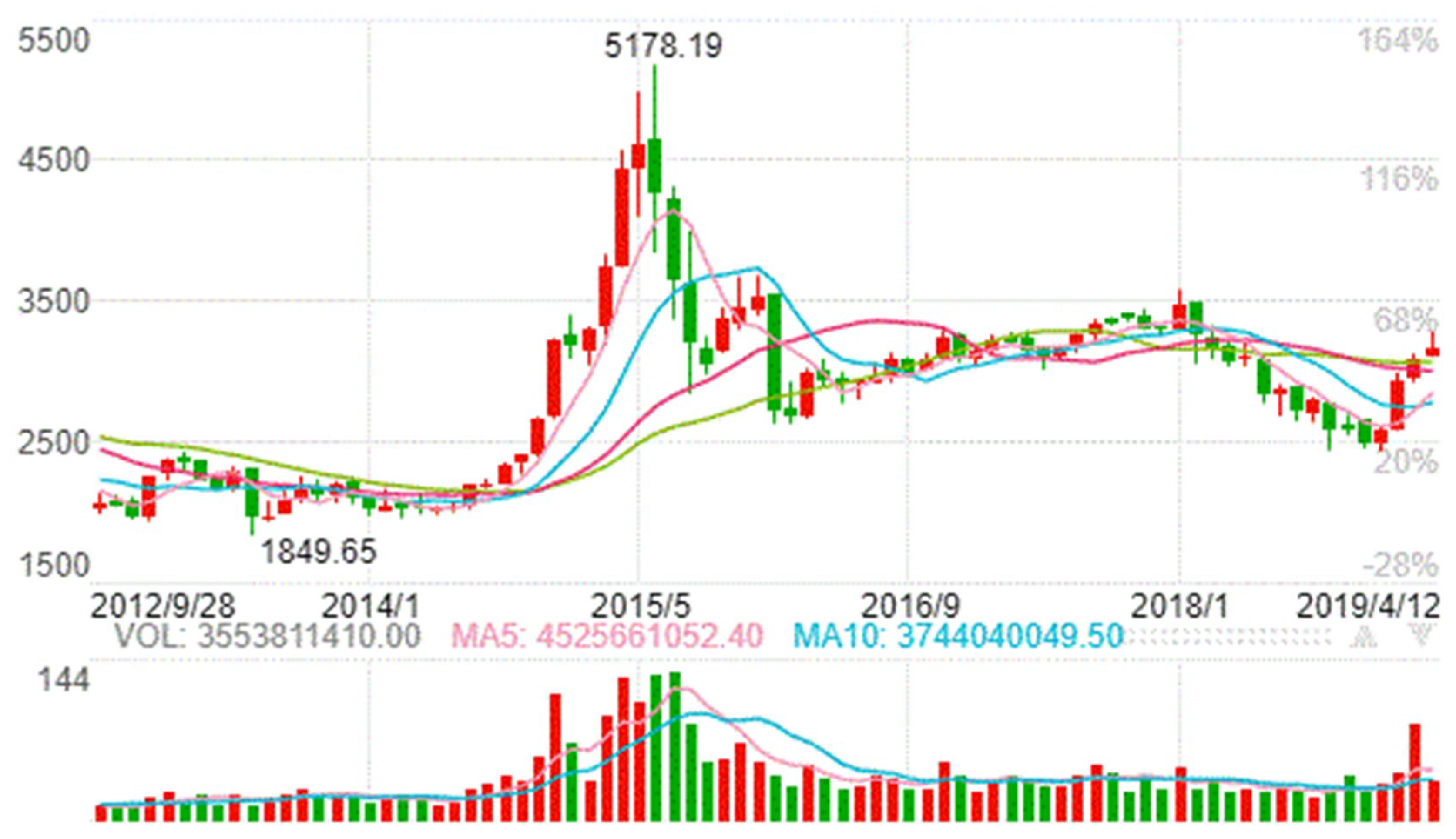
2016	0.282968	0.004437	1	1	0.728412	1	0.689547	1	1

, the efficiencies on the capital market are not DEA valid except for that of 2015. In combination with Figure 1, this further reveals that loose monetary policy has led to an upturn of the bonds market, volatile leverages and a fluctuant stock market. Beginning in 2014, China’s central bank imposed an interest rate cap through SLF, guided by a declining interbank rate and a lowering of the repo rate, and officially announced an interest cut in November that year. The extension of the loose period in the first half of 2015 resulted in a continuously bullish bond market. But after the loose period was renewed in August, the stock market became more fluctuant, and the accumulated effect of the loose monetary policy and high leverage ratio gave rise to a “raging” bull market. However, the abrupt changes in the expected looseness in the middle of the year, as well as the continuous deleveraging initiative, caused a plummet of stock market. The cut in interest rate and required reserve ratio (RRR) at the end of August portended a renewal of the loose period; in the meantime, the clearance of share financing that drew to an end in September, helping the stock market gradually recover from its crash. The efficiencies of fiscal and monetary policies of the ensuing year 2016 on the capital market were reduced to the minimum. As such, solely relying on loose monetary policy to inject vitality cannot ensure long-term stable development of the capital market. The supply-side structural reform initiated in 2015 represented a positive signal to reduce financing costs of the firms, strengthen financial support to the real economy, increase corporate competitiveness and reduce their taxation burdens. As indicated by the analysis of this paper, one of the goals of the supply-side reform is to moderate the substitutability and weights of factors pertinent to fiscal and monetary policies, thereby increasing the efficiency of fiscal and monetary policies on the capital market so that better services can be delivered to microeconomy.

4.3. Projection Analysis

Project analysis enables the identification of specific causes to the DEA-invalidity of DMUs, as well as directions towards which improvements can be made. As the windows-EBMb model incorporates the strengths of both radial and non-radial estimations, the input redundancy and output deficiency values are mainly comprised of proportionate movement and slack movement. The original value plus proportionate movement plus slack movement equals to Projection, and proportionate movement plus slack movement equals to value required to be moved, where Projection is at its optimal value. According to the output results of the model, we selected the data of China and respectively obtained the mean value of the next year’s efficiency, slack and projection under each window, yielding the following

Table 13. Efficiency movement of China based on windows-EBMb.

		Projection
	Efficiency	(I1)	(I2)	(I3-1)	(O1)	(O2)	(O3)
CHN {2008}	0.900597	8.27207 × 1011	4.26184 × 1011	6.27966 × 1012	4.59821 × 1012	5.80174 × 1012	1.02555 × 1013
CHN {2009}	0.866745	9.70089 × 1011	4.56822 × 1011	7.64398 × 1012	5.10995 × 1012	6.46725 × 1012	8.75839 × 1012
CHN {2010}	0.877352	1.16698 × 1012	5.46466 × 1011	9.42487 × 1012	6.10062 × 1012	7.48602 × 1012	9.59927 × 1012
CHN {2011}	0.889701	1.50756 × 1012	6.94391 × 1011	1.17515 × 1013	7.57255 × 1012	9.7348 × 1012	1.11581 × 1013
CHN {2012}	0.905876	1.718 × 1012	7.95248 × 1011	1.40239 × 1013	8.56055 × 1012	1.09425 × 1013	1.20568 × 1013
CHN {2013}	0.952684	1.79584 × 1012	9.08589 × 1011	1.7113 × 1013	9.60722 × 1012	1.53338 × 1013	1.1609 × 1013
CHN {2014}	0.969515	1.82343 × 1012	9.88249 × 1011	1.91174 × 1013	1.04824 × 1013	2.13304 × 1013	1.19593 × 1013
CHN {2015}	1	2.82421 × 1012	1.03723 × 1012	2.23569 × 1013	1.10647 × 1013	8.18802 × 1012	3.9326 × 1013
CHN {2016}	0.682987	1.93736 × 1012	1.36884 × 1012	1.59944 × 1013	1.1191 × 1013	2.0548 × 1013	1.82413 × 1013
		Input movement			Output movement
		(I1)	(I2)	(I3-1)	(O1)	(O2)	(O3)
CHN {2008}		−7.3576 × 1010	−3.7907 × 1010	−5.58544 × 1011	0	4.02295 × 1012	6.35043 × 1012
CHN {2009}		−1.46812 × 1011	−6.913 × 1010	−1.28866 × 1012	0	2.89409 × 1012	9.27618 × 1011
CHN {2010}		−1.605 × 1011	−7.516 × 1010	−1.29625 × 1012	0	3.45818 × 1012	1.34153 × 1012
CHN {2011}		−1.83193 × 1011	−8.438 × 1010	−1.428 × 1012	0	6.32269 × 1012	4.48408 × 1012
CHN {2012}		−2.77356 × 1011	−7.988 × 1010	−1.4087 × 1012	0	7.24509 × 1012	7.02962 × 1012
CHN {2013}		−4.67178 × 1011	−3.962 × 1010	−7.46247 × 1011	0	1.13846 × 1013	3.91302 × 1012
CHN {2014}		−6.47282 × 1011	−2.565 × 1010	−8.77667 × 1011	0	1.53254 × 1013	0
CHN {2015}		0	0	0	0	0	0
CHN {2016}		−8.88362 × 1011	−6.36707 × 1011	−7.33413 × 1012	0	1.32273 × 1013	0

(U.S. dollar). The specific operations are as follows: the projection is the mean of the corresponding yearly projection values of each factor across various windows; the input redundancy is the mean of the corresponding yearly value required to be moved of each input factor across all windows; and the output deficiency is the mean of the corresponding yearly value required to be moved of each output factor across all windows.

The reductions in fiscal expenditure (I1), total tax revenue (I2) and broad money supply (I3-1) lead to increases in GDP (O1), market value of listed domestic firms (O2) and yearly total value of shares traded (O3), and as the reduction of broad money supply (I3-1) intensifies, the growth of (O2) and (O3) becomes more evident, indicating a significant substitutional effect of fiscal tax policy adjustment to the factor of broad money supply.

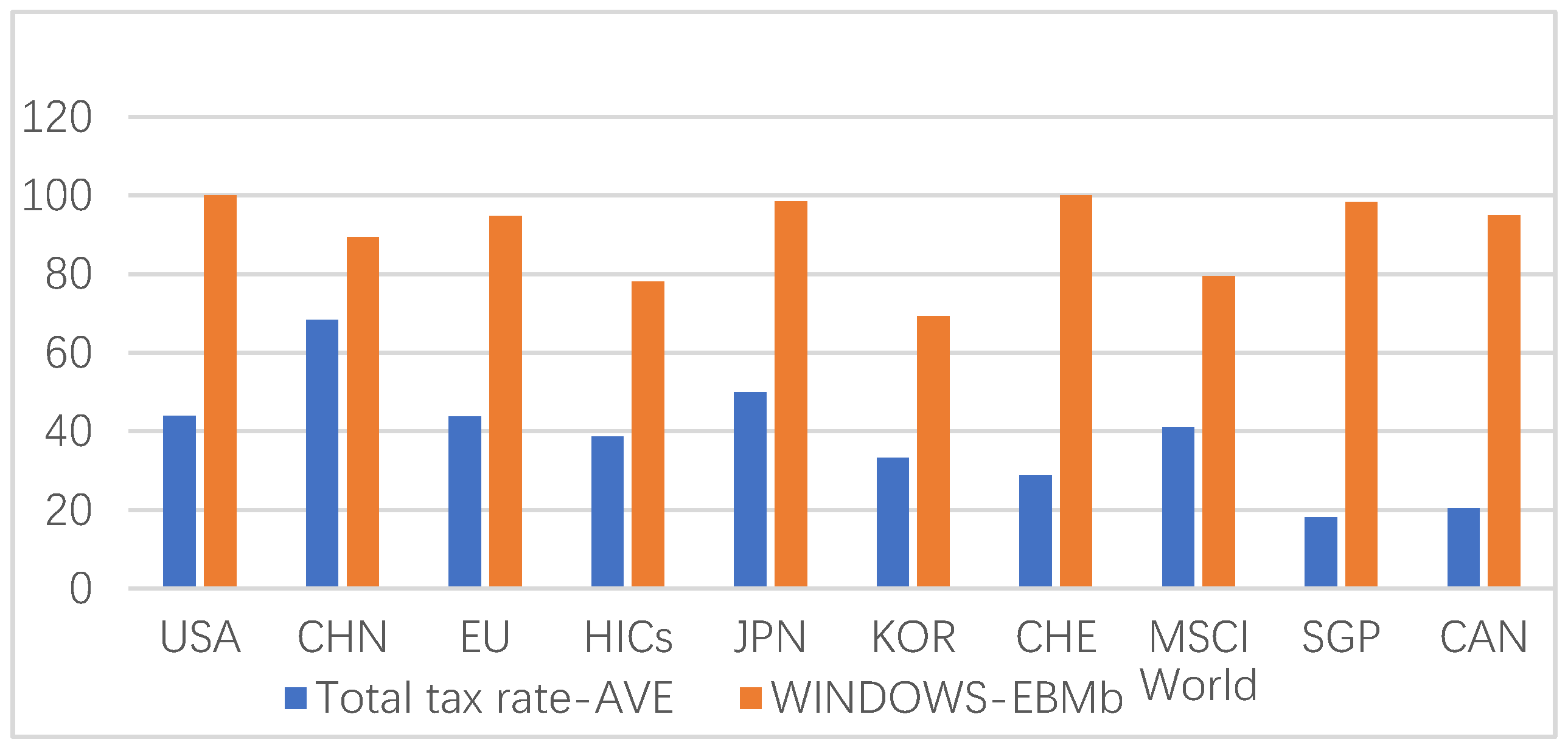
We selected the mean value of the averaged total tax rate of China, a few developed countries, high-income countries and the world between 2013 and 2016, and compared it with those efficiency obtained from the windows-EBMb model during the same period. We converted both sets of data, efficiency and tax rates into percentages as shown in Figure 2. Total tax rate measures the percentage of the payments against business profit of a firm. The withheld taxes (e.g., personal income tax) or taxes collected or remitted to tax authorities (e.g., VAT, sales tax or commodity or service taxes) are excluded. The total tax rate of China exceeds those of developed countries and the global average by more than half, indicating that Chinese firms are subject to heavier tax burdens; and a positive correlation between total tax rate and efficiency has yet to be made. Lowering the enterprise income tax would play an evident role in stimulating firms’ proactiveness and improving their competence as participants of the capital market. In addition, a cut in enterprise income tax can also be a foundation for reducing excess money supply, thereby allowing the disposable income of firms and their employees to come from the firms themselves, instead of excess money supply, further reducing the risk of inflation. As such, high taxes have not produced any positive effect on improving the activeness of China’s capital market, and there is still great room to deepen supply-side reform; thus presenting an immense space for China’s capital market to gain sustainable development.

5. Conclusions and Discussion

5.1. Empirical Conclusion

In this paper, the main fiscal and monetary policies of major countries and economies between 2008 and 2016 are selected as input factors and the GDP, market value of listed domestic firms and total value of shares traded as output factors in an analysis of the efficiency of these policies on the activeness of the capital market, represented by the stock market, by using the windows-DEA model and non-oriented EBM model. The results show that China’s fiscal and monetary policy measures have a relatively low influencing efficiency on the activeness of its capital market, and the efficiencies of DMUs differ significantly in contrast with those of developed countries, which are evidently higher than China and the global average. Measures for improvement are proposed.

(1) Although this paper uses two monetary policy indicators to test the robustness of the model, the focus of the analysis has always been on the supply side. Among the three input factors, fiscal expenditure, broad money supply or interest rate can be understood as the demand side, while tax reduction is a measure of supply-side reform. The results of our analysis suggest that tax reduction can replace fiscal expenditure and monetary or lower interest rates to stimulate the activity of capital markets.

(2) Taking China as an example, the analysis of the improvement measures under the EBMb model also shows that tax reduction, fiscal expenditure reduction and monetary overissuance, or the adjustment of the nominal interest rate can stimulate the active capital market and stabilize the economic growth. In other words, supply-side measures such as tax cuts are more positive than demand-side measures, such as loose fiscal spending and loose monetary policy. This is due to a more positive effect on the structural adjustment of Chinese economic growth. The analysis of affinity index verifies the obvious substitution relationship between tax and excess money supply as input factors, indicating that high tax does not play a positive role in capital market efficiency.

5.2. Policy Proposals

Based on the analysis results of the above models, this paper argues that supply-side reform should be carried forward by increasing efforts to reduce taxes, and to substitute the excess money supply with a stepwise tax cut; gradually lowering personal income tax to increase household disposable income and to stimulate the population’s desire to consume and invest; reducing enterprise taxes to increase their disposable incomes and boost their enthusiasm for investment, thus increasing employee incomes and reducing inflation risks arising from an excess money supply. All these efforts could create new values, effectively increase firms’ market values and thus boost their proactiveness to engage in the capital market, thus injecting vitality to the capital market.

5.3. Shortcomings

(1) In consideration of the actual situation in China, only the stock market was selected as a representative to examine the activeness of the capital market, without taking other areas of the capital market into account.

Influences arising from market speculation, economic cycles and other factors were not taken into consideration when input and output indicators were selected.

(2) Among the input factors, the possibility that the fiscal expenditure factor could be an increasable factor is not considered.

(3) The above shortcomings will hopefully be addressed in upcoming studies.

References

1. People.cn. China’s Supply-Side Structural Reform. 2016. Available online: http://theory.people.com.cn/n1/2016/0216/c402459-28127989-3.html (accessed on 29 April 2019).
2. DaGong Finance and Economics, Mr. Chen Shiqing, a Well-Known Economist, on “New Structural Economics”. 2016. Available online: http://finance.takungpao.com/mjzl/mjhz/2016-06/3327822.html (accessed on 29 April 2019).
3. The Economic Journal, Structural Reform: Change What, How to Change—Interview with Li Zuojun, Deputy Director of the Institute of Resources and Environment, Development Research Center of the State Council. 2015. Available online: http://theory.people.com.cn/n/2015/1123/c40531-27843619.html (accessed on 29 April 2019).
4. Fang, C.; Guan, X.; Lu, S.; Zhou, M.; Deng, Y. Input–output efficiency of urban agglomerations in China: An application of data envelopment analysis (DEA). Urban Stud. 2013, 50, 2766–2790. [Google Scholar] [CrossRef]
5. Wu, Y. Has productivity contributed to China’s growth? Pac. Econ. Rev. 2003, 8, 15–30. [Google Scholar] [CrossRef]
6. Lábaj, M.; Luptáčik, M.; Nežinský, E. Data envelopment analysis for measuring economic growth in terms of welfare beyond GDP. Empirica 2014, 41, 407–424. [Google Scholar] [CrossRef] [Green Version]
7. Zhu, X. Understanding China’s growth: Past, present, and future. J. Econ. Perspect. 2012, 26, 103–124. [Google Scholar] [CrossRef]
8. Nie, P. Research on China’s Sustained Economic Growth. Ph.D. Thesis, Southwestern University of Finance and Economics, Chongqin, China, 2011; p. 255. [Google Scholar]
9. Tang, A.; Zhao, D. A comparative analysis on the factors promoting China’s economic growth based on demand. Energy Procedia 2011, 5, 1388–1393. [Google Scholar]
10. Zhang, P. Research on the Correlation between China’s Stock Market and Macro Economy. Ph.D. Thesis, Party School of the CPC Central Committee, Beijing, China, 2013; p. 199. [Google Scholar]
11. Charnes, A.; Cooper, W.W.; Rhodes, E. Measuring the efficiency of decision making units. Eur. J. Oper. Res. 1978, 2, 429–444. [Google Scholar] [CrossRef]
12. Cullinane, K.; Song, D.W.; Ji, P.; Wang, T.F. An Application of DEA Windows Analysis to Container Port Production Efficiency. Rev. Netw. Econ. 2004, 3, 184–206. [Google Scholar] [CrossRef]
13. Tone, K.; Tsutsui, M. An epsilon-based measure of efficiency in DEA—A third pole of technical efficiency. Eur. J. Oper. Res. 2010, 207, 1554–1563. [Google Scholar] [CrossRef]
14. Banker, R.D.; Charnes, A.; Cooper, W.W. Some models for estimating technical and scale inefficiencies in data envelopment analysis. Manag. Sci. 1984, 30, 1078–1092. [Google Scholar] [CrossRef]
15. Färe, R.; Grosskopf, S.; Lovell, C.A. Production Frontiers; Cambridge University Press: Cambridge, UK, 1994. [Google Scholar]
16. Cheng, G.; Qian, Z. An epsilon-based measure of efficiency in DEA—An alternative method for the affinity index. In Data Envelopment Analysis Method and MaxDEA Software; Intellectual Property Press: Beijing, China, 2014; Chapter 4. [Google Scholar]
17. Sina. Sina Finance Shanghai Composite Index. 2019. Available online: http://finance.sina.com.cn/realstock/company/sh000001/nc.shtml (accessed on 14 April 2019).
Figure 1. Monthly candlestick patterns and trading volume of Shanghai Composite Index [17].
Sustainability 11 03012 g001
Figure 2. Comparison of mean value of total tax rate of each DMU and W-EBMb average efficiency between 2013 and 2016.
Sustainability 11 03012 g002