Application of Wavelet-Based Maximum Likelihood Estimator in Measuring Market Risk for Fossil Fuel


Abstract
:1. Introduction
2. Related Literature
2.1. Long-Memory and Market Efficiency
2.2. The Hurst Index
3. Methods for Estimating Long-Memory in Financial Time Series
3.1. Conventional Methods
3.2. Wavelet-Based Maximum Likelihood Estimator
4. Estimators’ Performance Comparison
- All of the proposed methods seem to estimate parameter H effectively, in that they can detect the dependence structure of the simulated time series, with relatively small standard errors.
- The values of , and do not differ significantly between the cases of N = 50 and N = 500.
- The rescaled range method yields the least desirable performance in all simulated experiments. This is in contrast to many previous studies supporting the use of this method, yet it is in line with skeptics such as [34].
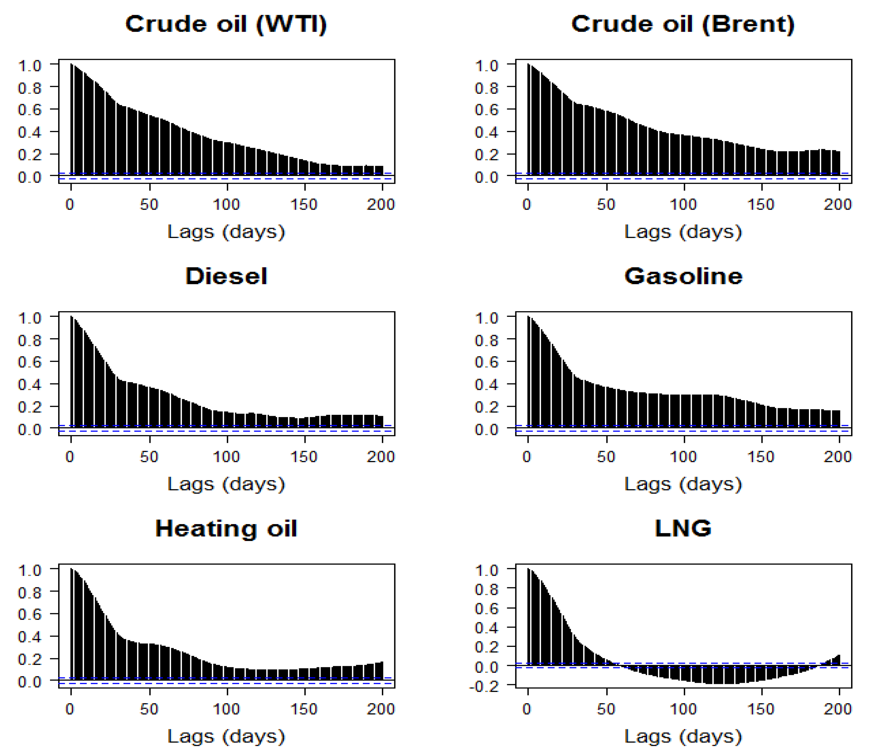
5. Application to Fossil Fuel Prices
6. Conclusions, Implications and Qualifications
Author Contributions
Funding
Acknowledgments
Conflicts of Interest
References
- Hurst, H. Long term storage capacity of reservoirs. Trans. Am. Soc. Civ. Eng. 1951, 116, 770–799. [Google Scholar]
- Gencay, R.; Selcuk, F.; Whitcher, B. An Introduction to Wavelets and Other Filtering Methods in Finance and Economics; Academic Press: San Diego, CA, USA, 2002. [Google Scholar]
- Samuelson, P.A. Proof that Properly Anticipated Prices Fluctuate Randomly. Ind. Manag. Rev. 1965, 6, 41–49. [Google Scholar]
- Fama, E.F. The Behavior of stock market prices. J. Bus. 1965, 38, 34–105. [Google Scholar] [CrossRef]
- Lo, A.W. Long-term memory in stock market prices. Econometrica 1991, 59, 1279–1313. [Google Scholar] [CrossRef]
- Jennergren, L.P.; Korsvold, P.E. Price formation in the Norwegian and Swedish stock markets: Some random walk tests. Swedish J. Econ. 1974, 76, 171–185. [Google Scholar] [CrossRef]
- Cootner, P.H. Common Elements in Futures Markets for Commodities and Bonds. Am. Econ. Rev. 1961, 51, 173–183. [Google Scholar]
- Fama, E.F.; French, K.R. Permanent and temporary components of stock prices. J. Polit. Econ. 1988, 96, 246–273. [Google Scholar] [CrossRef]
- Ding, Z.; Granger, C.W.J.; Engle, R.F. A long memory property of stock market returns and a new model. J. Empir. Finance 1993, 1, 83–106. [Google Scholar] [CrossRef]
- Andersen, T.G.; Bollerslev, T. Heterogeneous information arrivals and return volatility dynamics: Uncovering the long run in high frequency returns. J. Finance 1997, 52, 975–1005. [Google Scholar] [CrossRef]
- Mandelbrot, B.; Wallis, J.R. Noah, Joseph, and operational hydrology. Water Resources Res. 1968, 4, 909–918. [Google Scholar] [CrossRef]
- Peters, E. Chaos and Order in the Capital Markets: A New View of Cycles, Prices, and Market Volatility; John Wiley & Sons: New York, NY, USA, 1996. [Google Scholar]
- Lo, A.W.; MacKinlay, C.A. A Non-Random Walk Down Wall Street; Princeton University Press: Princeton, NJ, USA, 1999. [Google Scholar]
- Hull, M.; McGroarty, F. Do emerging markets become more efficient as they develop? Long memory persistence in equity indices. Emerging Markets Rev. 2013, 18, 45–61. [Google Scholar] [CrossRef]
- Grossman, S.J.; Stiglitz, J.E. On the impossibility of informationally efficient markets. Am. Econ. Rev. 1980, 70, 393–408. [Google Scholar]
- Lo, A.W. The adaptive markets hypothesis: Market efficiency from an evolutionary perspective. J. Portfolio Manag. 2004, 30, 15–29. [Google Scholar] [CrossRef]
- Choi, K.; Hammoudeh, S. Long memory in oil and refined products markets. Energy J. 2009, 30, 97–116. [Google Scholar] [CrossRef]
- Baillie, R.; Han, Y.-W.; Myers, R.; Song, J. Long memory models for daily and high frequency commodity futures returns. J. Futures Markets 2007, 27, 643–668. [Google Scholar] [CrossRef]
- Arouri, M.E.H.; Lahiani, A.; Lévy, A.; Nguyen, D.K. Forecasting the conditional volatility of oil spot and futures prices with structural breaks and long memory models. Energy Econ. 2012, 34, 283–293. [Google Scholar] [CrossRef]
- Charfeddine, L. True or spurious long memory in volatility: Further evidence on the energy futures markets. Energy Policy 2014, 71, 76–93. [Google Scholar] [CrossRef]
- Wang, Y.; Wu, C. Long memory in energy futures markets: Further evidence. Resources Policy 2012, 37, 261–272. [Google Scholar] [CrossRef]
- Di Sanzo, S. A Markov switching long memory model of crude oil price return volatility. Energy Econ. 2018, 74, 351–359. [Google Scholar] [CrossRef]
- Nademi, A.; Nademi, Y. Forecasting crude oil prices by a semiparametric Markov switching model: OPEC, WTI, and Brent cases. Energy Econ. 2018, 74, 757–766. [Google Scholar] [CrossRef]
- Dieker, A.B.; Mandjes, M. On spectral simulation of fractional Brownian motion. Probab. Eng. Informat. Sci. 2003, 17, 417–434. [Google Scholar] [CrossRef]
- Cox, D.R. Long-range Dependence: A Review. In Statistics: An Appraisal, Proceedings of a Conference Marking the 50th Anniversary of the Statistical Laboratory, Iowa State University, Ames, Iowa, 13–15 June 1983; David, H.A., David, H.T., Eds.; Iowa State University Press: Ames, IA, USA, 1984; pp. 55–74. [Google Scholar]
- Beran, J. Statistics for Long-Memory Processes; Chapman and Hall: New York, NY, USA, 1994. [Google Scholar]
- Mandelbrot, B.; Van Ness, J.W. Fractional Brownian motions, fractional noises and applications. SIAM Rev. 1968, 10, 422–437. [Google Scholar] [CrossRef]
- Mitra, S.K. Is Hurst exponent value useful in forecasting financial time series? Asian Soc. Sci. 2012, 8, 111–120. [Google Scholar] [CrossRef]
- Mandelbrot, B. Statistical methodology for nonperiodic cycles: From the covariance to R/S analysis. In Proceedings of the Annals of Economic and Social Measurement; National 579 Bureau of Economic Research: Stanford, CA, USA, 1972; Volume 1, pp. 259–290. [Google Scholar]
- Willinger, W.; Taqqu, M.S.; Teverovsky, V. Stock market prices and long-range dependence. Finance Stochastics 1999, 3, 1–13. [Google Scholar] [CrossRef]
- Teverovsky, V.; Taqqu, M. Testing for long-range dependence in the presence of shifting means or a slowly declining trend, using a variance-type estimator. J. Time Ser. Anal. 1997, 18, 279–304. [Google Scholar] [CrossRef]
- Higuchi, T. Approach to an irregular time series on the basis of the fractal theory. Phys. D Nonlinear Phenomena 1981, 31, 277–283. [Google Scholar] [CrossRef]
- Peng, C.K.; Buldyrev, S.V.; Havlin, S.; Simons, M.; Stanley, H.E.; Goldberger, A.L. Mosaic organization of DNA nucleotides. Phys. Rev. E 1994, 49, 1685–1689. [Google Scholar] [CrossRef]
- Taqqu, M.T.V.; Willinger, W. Estimators for long-range dependence: An empirical study. Fractals 1995, 3, 785–798. [Google Scholar] [CrossRef]
- In, F.; Kim, S. An Introduction to Wavelet Theory in Finance: A Wavelet Multiscale Approach; World Scientific: Singapore, 2013. [Google Scholar]
- Jensen, M.J. An alternative maximum likelihood estimator of long-memory processes using compactly supported wavelets. J. Econ. Dyn. Control 2000, 24, 361–387. [Google Scholar] [CrossRef]
- McLeod, B.; Hipel, K. Preservation of the rescaled adjusted range. Water Resources Res. 1978, 14, 491–518. [Google Scholar] [CrossRef]
- Resnick, S. Extreme Values, Regular Variation, and Point Processes; Springer: New York, NY, USA, 2007. [Google Scholar]
- Granger, C.W.J. The typical spectral shape of an economic variable. Econometrica 1966, 34, 150–161. [Google Scholar] [CrossRef]
- United States Energy Information Administration. Petroleum and other liquids. Available online: https://www.eia.gov/petroleum/data.php (accessed on 18 May 2019).
- Dickey, D.A.; Fuller, W.A. Distributions of the estimators for autoregressive time series with a unit root. J. Am. Stat. Assoc. 1979, 74, 427–431. [Google Scholar]
- Phillips, P.C.B.; Perron, P. Testing for a unit root in time series regression. Biometrika 1988, 75, 335–346. [Google Scholar] [CrossRef]
- Kwiatkowski, D.; Phillips, P.C.B.; Schmidt, P.; Shin, Y. Testing the null hypothesis of stationarity against the alternative of a unit root. J. Econometr. 1992, 54, 159–178. [Google Scholar] [CrossRef]
- Montgomery, S.L. Cheap oil is blocking progress on climate change. The Conversation [online] 2018, 12. Available online: https://theconversation.com/cheap-oil-is-blocking-progress-on-climate-change-108450 (accessed on 28 April 2019).
- Office of Energy Efficiency and Renewable Energy. About Two-Thirds of Transportation Energy Use is Gasoline for Light Vehicles; Office of Energy Efficiency and Renewable Energy: Washington, DC, USA, 2013.


| Hurst Exponent | Fractional Difference Parameter | Behavior of the Process |
|---|---|---|
| H ≤ 0 | d ≤ −1/2 | Non stationary |
| 0 < H < 1/2 | −1/2 < d < 0 | Anti-persistent, mean-reversing |
| H = 1/2 | d = 0 | Random, Brownian motion |
| 1/2 < H < 1 | 0 < d < 1/2 | Long-range dependence |
| H ≥ 1 | d ≥ 1/2 | Non stationary |
| Fractional Gaussian Noise | FARIMA (0, d, 0) | ||||||||||||
|---|---|---|---|---|---|---|---|---|---|---|---|---|---|
| H = 0.5 | H = 0.7 | H = 0.9 | H = 0.5 | H = 0.7 | H = 0.9 | ||||||||
| Method | Measurement | N = 50 | N = 500 | N = 50 | N = 500 | N = 50 | N = 500 | N = 50 | N = 500 | N = 50 | N = 500 | N = 50 | N = 500 |
| R/S | 0.564 | 0.563 | 0.717 | 0.713 | 0.823 | 0.830 | 0.560 | 0.571 | 0.682 | 0.703 | 0.846 | 0.828 | |
| 0.068 | 0.084 | 0.094 | 0.088 | 0.089 | 0.094 | 0.083 | 0.085 | 0.079 | 0.089 | 0.110 | 0.090 | ||
| 0.093 | 0.105 | 0.095 | 0.089 | 0.117 | 0.117 | 0.101 | 0.111 | 0.081 | 0.089 | 0.121 | 0.115 | ||
| aggVar | 0.493 | 0.498 | 0.685 | 0.684 | 0.847 | 0.843 | 0.495 | 0.496 | 0.690 | 0.686 | 0.844 | 0.843 | |
| 0.025 | 0.027 | 0.030 | 0.029 | 0.034 | 0.030 | 0.030 | 0.028 | 0.028 | 0.030 | 0.032 | 0.029 | ||
| 0.025 | 0.027 | 0.033 | 0.033 | 0.063 | 0.064 | 0.031 | 0.028 | 0.030 | 0.033 | 0.064 | 0.063 | ||
| diffaggVar | 0.508 | 0.518 | 0.715 | 0.710 | 0.899 | 0.902 | 0.515 | 0.511 | 0.719 | 0.706 | 0.901 | 0.900 | |
| 0.064 | 0.061 | 0.054 | 0.055 | 0.059 | 0.057 | 0.050 | 0.055 | 0.057 | 0.055 | 0.059 | 0.056 | ||
| 0.064 | 0.064 | 0.056 | 0.056 | 0.058 | 0.057 | 0.052 | 0.056 | 0.060 | 0.055 | 0.059 | 0.056 | ||
| AbaggVar | 0.498 | 0.502 | 0.691 | 0.690 | 0.853 | 0.849 | 0.497 | 0.501 | 0.695 | 0.692 | 0.850 | 0.849 | |
| 0.026 | 0.028 | 0.030 | 0.031 | 0.034 | 0.032 | 0.031 | 0.029 | 0.031 | 0.031 | 0.033 | 0.032 | ||
| 0.026 | 0.028 | 0.031 | 0.032 | 0.057 | 0.060 | 0.031 | 0.029 | 0.031 | 0.032 | 0.060 | 0.060 | ||
| Per | 0.497 | 0.501 | 0.705 | 0.706 | 0.912 | 0.912 | 0.498 | 0.499 | 0.705 | 0.704 | 0.908 | 0.909 | |
| 0.019 | 0.022 | 0.020 | 0.020 | 0.021 | 0.021 | 0.019 | 0.022 | 0.019 | 0.022 | 0.021 | 0.021 | ||
| 0.019 | 0.022 | 0.020 | 0.021 | 0.024 | 0.024 | 0.019 | 0.022 | 0.020 | 0.022 | 0.023 | 0.023 | ||
| modPer | 0.451 | 0.456 | 0.662 | 0.664 | 0.869 | 0.870 | 0.452 | 0.454 | 0.660 | 0.658 | 0.863 | 0.860 | |
| 0.023 | 0.022 | 0.024 | 0.022 | 0.024 | 0.022 | 0.020 | 0.023 | 0.023 | 0.022 | 0.023 | 0.022 | ||
| 0.054 | 0.049 | 0.045 | 0.042 | 0.039 | 0.037 | 0.052 | 0.052 | 0.046 | 0.047 | 0.044 | 0.045 | ||
| Peng | 0.489 | 0.491 | 0.688 | 0.688 | 0.886 | 0.885 | 0.487 | 0.489 | 0.676 | 0.677 | 0.873 | 0.874 | |
| 0.015 | 0.012 | 0.015 | 0.015 | 0.018 | 0.016 | 0.013 | 0.012 | 0.015 | 0.016 | 0.017 | 0.017 | ||
| 0.018 | 0.015 | 0.019 | 0.019 | 0.022 | 0.022 | 0.019 | 0.016 | 0.028 | 0.028 | 0.032 | 0.031 | ||
| Higuchi | 0.474 | 0.478 | 0.670 | 0.670 | 0.860 | 0.857 | 0.473 | 0.476 | 0.675 | 0.670 | 0.865 | 0.859 | |
| 0.017 | 0.019 | 0.025 | 0.025 | 0.036 | 0.042 | 0.023 | 0.020 | 0.029 | 0.026 | 0.044 | 0.041 | ||
| 0.031 | 0.029 | 0.039 | 0.039 | 0.053 | 0.060 | 0.035 | 0.031 | 0.039 | 0.040 | 0.056 | 0.058 | ||
| waveMLE | 0.497 | 0.501 | 0.725 | 0.726 | 0.915 | 0.915 | 0.500 | 0.500 | 0.694 | 0.694 | 0.895 | 0.891 | |
| 0.008 | 0.008 | 0.008 | 0.008 | 0.017 | 0.017 | 0.009 | 0.008 | 0.009 | 0.008 | 0.024 | 0.021 | ||
| 0.008 | 0.008 | 0.027 | 0.027 | 0.023 | 0.022 | 0.009 | 0.008 | 0.011 | 0.010 | 0.024 | 0.023 | ||
| Fractional Gaussian Noise | |||||
| Method | H = 0.5 | Method | H = 0.7 | Method | H = 0.9 |
| waveMLE | 0.00809 | Peng | 0.01948 | Peng | 0.0217846 |
| Peng | 0.015141 | Per | 0.021326 | waveMLE | 0.0223977 |
| Per | 0.021721 | waveMLE | 0.027468 | Per | 0.0237573 |
| aggVar | 0.0267 | AbaggVar | 0.032387 | modPer | 0.0372976 |
| AbaggVar | 0.027645 | aggVar | 0.033436 | diffaggVar | 0.0567174 |
| Higuchi | 0.029087 | Higuchi | 0.039072 | Higuchi | 0.0598122 |
| modPer | 0.049141 | modPer | 0.042152 | AbaggVar | 0.0602138 |
| diffaggVar | 0.063601 | diffaggVar | 0.055628 | aggVar | 0.0641194 |
| R/S | 0.105121 | R/S | 0.089366 | R/S | 0.1170989 |
| FARIMA (0, d, 0) | |||||
| Method | H = 0.5 | Method | H = 0.7 | Method | H = 0.9 |
| waveMLE | 0.008196 | waveMLE | 0.010249 | waveMLE | 0.0227378 |
| Peng | 0.016386 | Per | 0.021878 | Per | 0.0228976 |
| Per | 0.021512 | Peng | 0.028202 | Peng | 0.0314989 |
| aggVar | 0.028119 | AbaggVar | 0.032151 | modPer | 0.0452348 |
| AbaggVar | 0.029126 | aggVar | 0.033022 | diffaggVar | 0.0557743 |
| Higuchi | 0.031394 | Higuchi | 0.039716 | Higuchi | 0.0581878 |
| modPer | 0.051638 | modPer | 0.047401 | AbaggVar | 0.0602195 |
| diffaggVar | 0.055694 | diffaggVar | 0.055482 | aggVar | 0.0634601 |
| R/S | 0.110746 | R/S | 0.08907 | R/S | 0.1150482 |
| Crude Oil (WTI) | Crude Oil (Brent) | Diesel | Gasoline | Heating Oil | LNG | |
|---|---|---|---|---|---|---|
| A. Returns | ||||||
| Mean | 0.00 | 0.00 | 0.00 | 0.00 | 0.00 | 0.00 |
| Median | 0.00 | 0.00 | 0.00 | 0.00 | 0.00 | 0.00 |
| Variance | 0.00 | 0.00 | 0.00 | 0.00 | 0.00 | 0.00 |
| Skewness | −0.11 | −0.07 | 0.09 | −0.02 | −1.30 | 0.53 |
| Kurtosis | 4.48 | 4.85 | 10.96 | 5.75 | 36.58 | 23.36 |
| JB | 4,636.39 | 5,425.09 | 27,726.50 | 7,626.17 | 31,0451.74 | 12,6236.23 |
| (0.00) | (0.00) | (0.00) | (0.00) | (0.00) | (0.00) | |
| LB(21) | 49.22 | 52.96 | 58.48 | 59.98 | 63.28 | 269.94 |
| (0.00) | (0.00) | (0.00) | (0.00) | (0.00) | (0.00) | |
| B. Volatilities | ||||||
| Mean | 0.02 | 0.02 | 0.02 | 0.03 | 0.02 | 0.04 |
| Median | 0.02 | 0.02 | 0.02 | 0.02 | 0.02 | 0.03 |
| Variance | 0.00 | 0.00 | 0.00 | 0.00 | 0.00 | 0.00 |
| Skewness | 1.78 | 1.43 | 2.21 | 2.02 | 5.69 | 2.94 |
| Kurtosis | 4.35 | 3.59 | 8.77 | 7.93 | 52.33 | 11.73 |
| JB | 7,253.17 | 4,820.13 | 22,147.27 | 18,174.67 | 65,8570.09 | 39,502.69 |
| (0.00) | (0.00) | (0.00) | (0.00) | (0.00) | (0.00) | |
| LB(21) | 87,932.64 | 87,228.02 | 75,212.60 | 77,604.79 | 76,836.39 | 72,836.22 |
| (0.00) | (0.00) | (0.00) | (0.00) | (0.00) | (0.00) | |
| Crude Oil (WTI) | Crude Oil (Brent) | Diesel | Gasoline | Heating Oil | LNG | |
|---|---|---|---|---|---|---|
| A. Returns | ||||||
| ADF | −16.90 | −16.88 | −17.43 | −16.28 | −18.76 | −19.78 |
| (0.01) | (0.01) | (0.01) | (0.01) | (0.01) | (0.01) | |
| PP | −5402.46 | −5459.67 | −6006.09 | −5192.76 | −5566.76 | −4420.88 |
| (0.01) | (0.01) | (0.01) | (0.01) | (0.01) | (0.01) | |
| KPSS | 0.08 | 0.08 | 0.05 | 0.05 | 0.07 | 0.03 |
| (0.10) | (0.10) | (0.10) | (0.10) | (0.10) | (0.10) | |
| B. Volatilities | ||||||
| ADF | −6.32 | −6.59 | −8.29 | −8.89 | −9.36 | −10.14 |
| (0.01) | (0.01) | (0.01) | (0.01) | (0.01) | (0.01) | |
| PP | −60.94 | −65.79 | −99.93 | −97.12 | −94.14 | −101.89 |
| (0.01) | (0.01) | (0.01) | (0.01) | (0.01) | (0.01) | |
| KPSS | 1.90 | 3.44 | 1.94 | 4.04 | 2.95 | 0.39 |
| (0.01) | (0.01) | (0.01) | (0.01) | (0.01) | (0.08) | |
| Crude Oil (WTI) | Crude Oil (Brent) | Diesel | Gasoline | Heating Oil | LNG | |
|---|---|---|---|---|---|---|
| Returns | 0.5 | 0.48 | 0.51 | 0.54 | 0.52 | 0.38 |
| Volatilities | 0.79 | 0.8 | 0.77 | 0.79 | 0.79 | 0.78 |
© 2019 by the authors. Licensee MDPI, Basel, Switzerland. This article is an open access article distributed under the terms and conditions of the Creative Commons Attribution (CC BY) license (http://creativecommons.org/licenses/by/4.0/).
Share and Cite
Vo, L.H.; Vo, D.H. Application of Wavelet-Based Maximum Likelihood Estimator in Measuring Market Risk for Fossil Fuel. Sustainability 2019, 11, 2843. https://doi.org/10.3390/su11102843
Vo LH, Vo DH. Application of Wavelet-Based Maximum Likelihood Estimator in Measuring Market Risk for Fossil Fuel. Sustainability. 2019; 11(10):2843. https://doi.org/10.3390/su11102843
Chicago/Turabian StyleVo, Long Hai, and Duc Hong Vo. 2019. "Application of Wavelet-Based Maximum Likelihood Estimator in Measuring Market Risk for Fossil Fuel" Sustainability 11, no. 10: 2843. https://doi.org/10.3390/su11102843
APA StyleVo, L. H., & Vo, D. H. (2019). Application of Wavelet-Based Maximum Likelihood Estimator in Measuring Market Risk for Fossil Fuel. Sustainability, 11(10), 2843. https://doi.org/10.3390/su11102843