1. Introduction
China is a large agricultural country with a population of over 560 million farmers [
1]. However, the per-capita income in the countryside is only one third of that in cities [
2]. Wages, household businesses, and farming are three main components of their incomes [
3]. Agriculture is a fundamental industry that plays an increasingly important role in the national economy and in people’s livelihoods [
4]. However, there have been thousands of wasted agricultural products in recent years [
5]. For example, more than 100,000 tons of pitaya in Foshan, China were unsold and released to fish ponds in 2015 due to the high amount of decay and low market demand [
6]. Thus, the profit of farming is only a quarter of the total profit [
3]. Moreover, the market is mostly dominated by offline retailers or giant wholesalers, who usually hold more power to be the leader in the supply chain [
7]. Moreover, few farmers choose the online channel to enlarge their market. Thus, it is essential to help the farmers expand their market and find a better way to get more profit. To improve the farmer’s profits, the government implemented the 13th Five-Year Plan, in which the agricultural products industry and the rural e-commerce developing plan are emphasized [
8]. New sales channels are encouraged in the plan, which also creates a good external condition to carry out online sales.
However, agricultural activities, including production, storage, and sales, contribute a significant share of greenhouse gas emissions and concurrently represent a carbon dioxide sink [
9]. As an important part of environmental issues, global warming, which is mainly caused by carbon emissions from human activities, is further intensifying. In order to curb carbon emissions, governments around the world have developed and applied relevant low-carbon policies and regulations, among which the cap-and-trade and the carbon tax are two main popular regulations [
10]. However, the carbon tax is extensively advocated, since it is regarded as the lowest cost emission reduction measure [
11]. As one of the ten world’s highest carbon emission countries, China also concentrates on the environmental problems [
12]. The government has imposed a carbon tax on eight industries since 2016, including petrochemical, power, aviation, and so on, and the carbon tax is expected to cover all the enterprises and the industries in 2020 [
13]. Therefore, the agricultural industry will also be involved in the near future. It is important to take environmental issues into consideration when the farmer is facing channel selection.
Based on the above background, the channel selection is quite significant under the carbon tax policy and the Internet economy background for both farmers and the government. Many scholars have conducted in-depth research on carbon management. For example, the carbon footprint analysis is carried out in different supply chains, such as the milk supply chain, the aquatic products supply chain, the fruit supply chain, and so on [
14,
15,
16,
17]. Enterprises’ decisions of carbon reduction investment were also studied by Wang et al. [
18] and Krass et al. [
19]. Additionally, there has been a great deal of research done regarding the channel selections. For example, producers’ and factories’ channel selections among traditional offline channels and other channels were investigated [
20,
21,
22,
23]. Moreover, the conflict between the new channel and the traditional one was also studied [
24]. These studies are profound and enlightening. However, there are few systematic studies on the impact of carbon emissions on the farmer’s channel selection, especially considering the deterioration rate of agricultural products and the carbon tax on supply chain members.
The goal of this paper is to fill in the gap by finding out the optimal producing and sales plan for the farmer, then comparing and analyzing the carbon emissions of different channels for the government. Therefore, this paper compares and analyzes the optimal profits that the farmer can obtain through different channels when the yield is known. At the same time, this paper considers the carbon emissions under sustainable development and evaluates the environmental factors of different channels to support the country’s sustainable development. In order to do the above analysis, we study three different channels to discuss the farmer’s selection with or without the carbon tax policy. The impact of the downstream decisions is also considered.
The rest of this paper is presented as follows. In
Section 2, the literature review is provided as our theoretical foundation. In
Section 3, the assumptions and the basic models are shown.
Section 4 analyzes the model and describes some theorems we obtained. The numerical analysis and the sensitivity analysis are presented in
Section 5. Finally, we describe the conclusion and future research.
2. Literature Review
This research is related to two streams of literature. Firstly, we make the analysis on carbon footprint and low-carbon management. Then, we review the articles about channel selection decisions made by various supply chain members. We present a concise review below.
2.1. Carbon Footprint and Low-Carbon Management
Some scholars have researched the environmental impact of supply chain members’ operational decisions. Two main branches are studying the carbon footprint and the low-carbon supply chain management.
The existing carbon footprint analysis of perishable agricultural products is mostly carried out and analyzed based on the PAS2050-based life cycle assessment (LCA) jointly issued by the British Standards Institute. The LCA is one of the most widely used methods for quantifying the environmental influence of products throughout its entire life cycle [
25]. Benjaafar et al. [
14] analyzed the carbon footprint and applied it to construct a measurement model. Meanwhile, they selected the milk supply chain as an example analysis object. Strutt et al. [
15] used the life cycle method to evaluate and study the carbon footprint of aquatic products. Al-Mansour et al. [
9] described the calculation model of agricultural carbon footprint and introduced the research results of grain and fruit carbon footprint. They also proposed a new farming method to reduce carbon emissions referring to the life cycle of agricultural products. Cappelletti et al. [
16] used the LCA method to evaluate the carbon emissions in the production and the processing of Italian edible olives. Jesper et al. [
17] evaluated the carbon emissions of the production and the processing of traditional brown bread. Chojnacka et al. [
26] considered the carbon emission of production, transportation, and use of fertilizers based on the LCA analytical method. Yan et al. [
27] researched the carbon footprint of the grain crop production process with the farm survey data from eastern China. They also compared the carbon footprint of three major grain crops (rice, wheat, and maize). Zhang et al. [
28] concentrated on the production of maize on the Loess Plateau of China to figure out the carbon footprint. They concluded that the large potential for improvement could be realized by integrating crops, nutrients, and water management.
On the literature related to low-carbon emission supply chain management, Wang et al. [
18] analyzed the supply chain involving a manufacturer and a retailer, then found that cost-sharing and wholesale price contracts could effectively encourage manufacturers to invest in carbon-reduction equipment. Carrillo et al. [
29] considered the impact of environmentally relevant factors on costs in a two-channel supply chain problem while focusing on the channel decision-making issues of retailers in the supply chain. Krass et al. [
19] also studied corporate decision-making in the low-carbon context of the supply chain and found that the increase in initial carbon costs would motivate companies to invest in and acquire low-carbon facilities. Hua et al. [
30] found that carbon trading policies had a larger impact on corporate decision-making. Tsai et al. [
31] analyzed the carbon emissions in different stages of tire production in order to lower the total carbon emissions of products. Activity-based costing (ABC) was adopted to assess green quality management and production cost. Thus far, research on low-carbon supply chain management has continued to expand. For example, Yang et al. [
32] added the low-carbon preference of consumers into consideration. Ji et al. [
20] focused on the low-carbon strategy of retailers and manufacturers while considering consumers’ low-carbon preferences and corporate carbon reduction strategies. Martin et al. [
21] found that the carbon tax had a strong negative impact on energy intensity and electricity use for manufacturers. Chen et al. [
22] used evolutionary game theory to study manufacturers’ behavioral strategies under carbon taxes and subsidies. They found that the carbon taxes levied by governments proved more effective in encouraging low-carbon manufacturing than governments subsidizing the low-carbon technology. Wang et al. [
23] constructed a decentralized supply chain using the three-stage Stackelberg game model and the two-stage Stackelberg game model under the carbon tax. They found that both the environmental performance and the financial performance of the supply chain were better off when the supply chain members had distributed pricing powers.
Most of the above literature considered the effect of supply chain strategies on carbon emissions. Few researchers used LCA to analyze the carbon emissions. In this paper, we combine the carbon footprint with the farmer’s channel selection strategies. The impact of carbon tax on supply chain members’ decisions and profit is also considered.
2.2. Channel Selection
Another study similar to our research is channel selection. In recent years, channel selection has gradually become a hot topic, especially in the background of internet economy.
Many scholars have studied channel selection from the perspective of decision makers. At present, most of these studies are based on retailers, manufacturers, or suppliers. For example, Xu et al. [
33] discovered that the use of new channels may lower the product’s price. Yang et al. [
3] analyzed and compared the channels between manufacturers in the retailer channel, the online channel, and dual channels, considering the cap-and-trade regulation. Khouja et al. [
34] analyzed the manufacturer’s channel selections and manufacturer’s pricing decisions and found important factors affecting the choice of manufacturers’ channels. Chiang et al. [
35] found that it was beneficial for suppliers to establish a direct sales channel to compete with their corresponding retailers. Wang et al. [
36] found that, for retailers with multi-channel sales, the difference in operating costs between different channels was an important issue affecting retailers’ channel selections. Fruchter et al. [
33] considered a channel choice for a manufacturer that could sell a product through retail channels and online channels simultaneously. Yang et al. [
37] developed a supplier–retailer fresh product supply chain under three modes, and they investigated the optimal pricing and freshness-keeping decisions for different participators. They found the optimal modes for supplier, retailer, and consumer surplus. In addition to the research on channel selection, there have been many studies on channel conflicts. For example, on retailer channel selection, Abdelsalam et al. [
38] found that the new sales channels would reduce the sales of the original sales channels. This would reduce the total sales profit rather than increase the total profit.
There is some research about farmer’s channel selection. For example, Hao et al. [
39] took the sales of apples by farmers in Shanxi and Shaanxi provinces of China as an example, and investigated the factors affecting the selections of sales channels by farmers. They found that the acquisition of membership in cooperatives had no significant impact on the sales of products. Digvijay et al. [
40] studied the influence of transportation and communication networks on farmers’ choices of channels when selling wheat and rice. They found that information and transportation were two main factors that affected their benefits on price, and information was more sensitive to their decisions.
Therefore, there are many studies related to channel selections. However, most of the research has focused on large manufacturers and retailers, both of which are in a dominant position in the supply chain. There are few studies focusing on the strategies of disadvantaged members in the supply chain after taking into account the decisions of other members, especially the studies concentrating on the farmer’s decisions. Additionally, the studies linked to the farmer are mostly qualitative. Moreover, the studies on comparisons among different channels are still insufficient and are far from abundant. Little research has systematically combined the channel selection problem with the perishable products and the carbon tax. In this paper, we expand the research field to the farmer’s channel selection combined with the environmental issues, trying to provide quantitative research about the farmer’s channel selection. A quantitative profit model is given as the basis for optimal decisions. Moreover, from the perspective of reducing carbon emissions, carbon tax, carbon footprint, and channel selection are combined, which enables governments to make decisions on sustainability by adjusting farmer’s channel selection.
3. The Models
3.1. System Boundaries and Assumptions
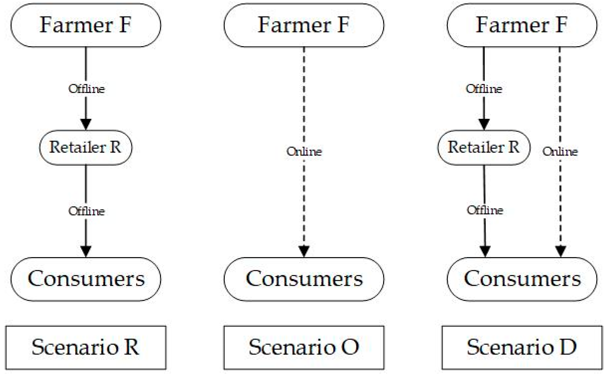
There are three types of channels in this paper. In the online channel, simplified as Scenario O, a single channel is considered where consumers purchase products from the farmer directly. In the retail channel, referred to as Scenario R, a two-stage agricultural supply chain consisting of one farmer and one retailer is discussed. The farmer as the supplier is always the vulnerable one confronted with more risk, and among all the option contracts led by different leaders, the option quantity led by the retailer is the highest [
37]. The dual channels, expressed as Scenario D, include two situations above. The general constructions of three channels are as follows in
Figure 1:
Before analyzing the model, assumptions are presented as follows:
- (1)
In the two-stage supply chain where the retailer is powerful enough, the shortage of farmer’s supply is not considered [
41].
- (2)
There are two main categories of measures on demand: stochastic demand and deterministic demand [
42]. In this paper, the demand is regarded as a constant.
- (3)
Inventory models are classified with simultaneous deteriorating rate and fixed lifetime with random lifetime [
43]. We assume the deterioration rate is a constant.
- (4)
Compared with the cost in production, the farmer’s inventory cost is ignored.
- (5)
The third-party logistics—but not the retailer—is responsible for carbon emissions when the agricultural products are transported.
- (6)
The carbon emissions are linear with product quantity [
10].
3.2. Methodological Approach
In this paper, we mainly adopt two kinds of methodological approaches, including the Stackelberg game model and the inventory model for perishable products, which are illustrated respectively below.
The supply chain in the retail channel of this paper includes two members, which are the farmer and the retailer. The farmer is much more powerless, and the retailer has the absolute initiative [
7]. The supply chain is mainly analyzed with the Stackelberg game model, in which there is a leader and others follow his decisions [
7]. In this paper, the retailer firstly makes optimal decisions, deciding the order quantity that depends on the optimal sales period and signing up the contracts with the farmer. Referring to the retailer’s choice, the farmer would accept the contract and decide its yield. When the carbon tax is imposed on the retailer, the retailer would firstly adjust their decisions to a new optimal value, and then the decisions and the profit of the farmer would accordingly change. A similar situation can be found in Yang et al. [
10].
Because the sales and the production of the agricultural products are seasonal, and the products are perishable, conventional supply chain strategies are inappropriate, since the products’ values change over time [
44]. The amount to purchase in the harvest season as well as each sales period strongly impact the profit for a wholesaler and a retailer [
5]. Thus, this paper adopts the inventory model for perishable goods to model the optimal strategies of the farmer and the retailer. The same process can be found in Biswajit et al. [
45], Qin et al. [
46], and Giri et al. [
47].
3.3. Model Description
All notations used in the models are summarized in
Table 1.
In our model, the demand is a constant. In the online channel, the farmer’s inventory can be applied to the inventory model of perishable products. The inventory level of the retailer and the farmer is modeled as Ghare and Schrader did [
48].
For the farmer, the boundary condition is that the inventory level equals with the yield of the farmer. Thus, the retailer’s order quantity is the inventory level at the beginning of the sales period. After the order is received from the retailer, the farmer starts to produce. In the dual channels, we introduce the farmer’s new decision variable—the proportion of the products sold online. Once the farmer chooses the dual channels, he needs to decide the proportion to reach the optimal profit.
To find the farmer’s optimal profit, we analyze the retailer’s optimal decisions. For the retailer, inventory cost, raw material cost, and deterioration cost are three main cost resources without carbon tax. When the carbon tax carries out, the carbon cost will also be considered. In the two cases, the total revenue is determined by the demand rate and the sales period. Therefore, the retailer’s profit function can be obtained as follows:
Then, all the functions of revenue and cost among three channels are listed. For the online channel, the demand comes from customers, and the cost mainly comes from the productive process. For the retail channel, the retailer’s orders are direct demands for the farmer; cost is also the production cost. Finally, the demand consists of both the customers’ demands and the retailer’s orders. Thus, we can get the farmer’s profit functions in different channels as follows:
Finally, to compare the emissions in different channels, we study every component. The carbon emissions consist of transporting emissions
, inventory emissions
, and deterioration emissions
. We exclude the production emissions because they are constant in three channels for the same yield. Additionally, there is a huge difference between online transporting emissions and offline transporting emissions due to the various transport mileage. The total emissions are linear with the quantity of products, thus we can conclude the total emissions of different channels as follows:
3.4. Model Formulation and Analysis
3.4.1. Without Carbon Tax
Without carbon tax, the farmer’s and the retailer’s profit functions can be described as
Table 2, and the corresponding proof is shown in
Appendix A.1.
Table 3 explains the decision variables,
Table 4 solves the farmer’s optimal profits, and the carbon emissions of the entire supply chain are presented in
Table 5.
3.4.2. With Carbon Tax
With the carbon tax, the farmer’s and the retailer’s profit functions can be written as
Table 6, and the corresponding proof is shown in
Appendix A.2.
Table 7 presents the decision variables,
Table 8 solves the optimal profits, and
Table 9 shows the carbon emissions of the entire supply chain.
4. The Results and Analyses
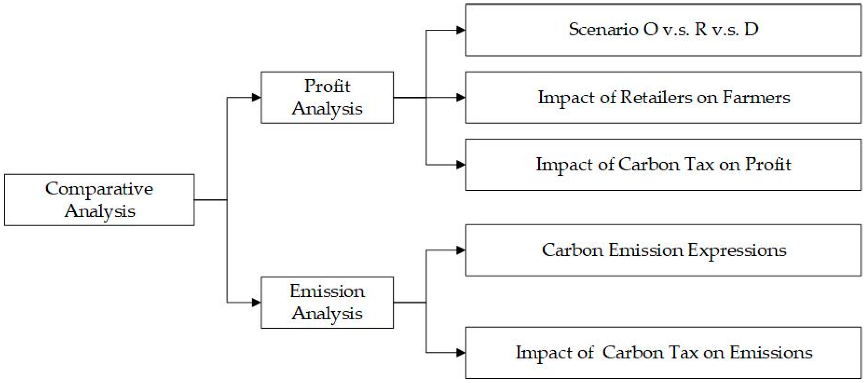
This section focuses on the comparisons of the profit and the carbon emissions among different channels. Firstly, the profit of each channel is analyzed. Then, the comparative analyses among different channels’ profits are carried out. Secondly, the profit analysis with carbon cost is realized in the same way. Finally, the carbon emissions of two cases are analyzed and compared. The concrete analysis and comparison methods are shown in
Figure 2.
4.1. Profit Analysis
We determine the relationship between channels’ profits and yield of products in two cases in which carbon tax is considered or not and find the critical values that determine the decisions on channel selection in these two cases. During the process, we also analyze the impact of the retailer’s relevant decision variables. The proof of the solution process of lemmas and theorems is shown in
Appendix B.
4.1.1. Profit functions and channel selection
We describe the relationship between profit and yield among three channels. In doing so, we find that the optimal channel varies when yield grows. A concern on how to choose the optimal channel arises and is discussed in the following paragraphs.
Lemma 1. With or without carbon tax policy, the relationship between the farmer’s profits from all channels and the output of agricultural products is as follows:
(1) If ; Otherwise, ; (2) ; (3) If , ; Otherwise .
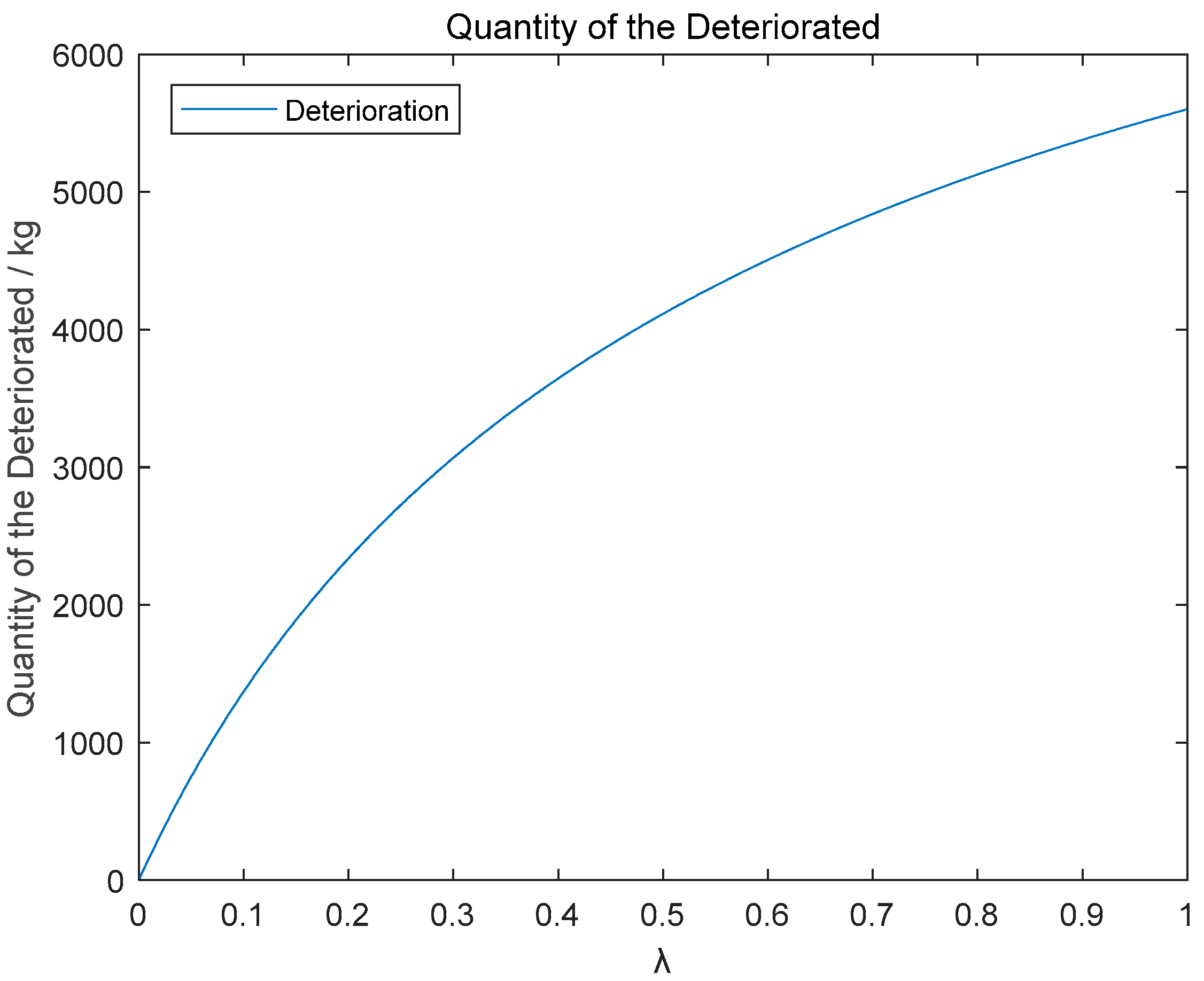
Lemma 1 provides some insights: (1) for the online channel, when the yield is less than a certain value, the farmer’s profits will increase with the increase of yield. On the contrary, the profit is negatively correlated with yield, and the maximum profit is obtained. The reason for this phenomenon is that the quantity of rotten products is relatively low when the farmer’s output is small, and the increased sales can positively compensate for the cost of rotten products. When the farmer’s output is large, the negative effect brought by the rotten products will exceed the positive effect brought by the increased sales; (2) for the retail channel, the profit of the farmer is a first-order monotone increasing function of output . This is because the farmer will negotiate with the retailer in advance, which ensures the stability of offline sales. Therefore, as long as the wholesale price is higher than the cost price, larger sales can make more profits; (3) for the dual channels, there is a positive correlation between the profit and the output when the products are less than a certain yield value, while the correlation is negative when the yield of products is high.
Theorem 1. For a certain yield of agricultural products , the farmer’s channels of optimal profit with or without carbon tax are as follows. There certainly exists two values of : and , in which . The farmer selects the online channel if , chooses the dual channels if , and adopts the retail channel if .
There are two values of yield ( and ), enabling the farmer to choose the online channel to get the maximum profit when the yield is lower than . When the yield is between and , dual channels are the best channel for the farmer. When the yield is more than , adopting the retail channel allows the farmer to receive the optimal profit. Thus, the farmer could draw up a suitable production plan and sales plan in the next period.
4.1.2. Impact of retailer’s decisions on the farmer
When the retailer is in the downstream of a supply chain, its decisions bring an impact on the farmer’s profit in the upper stream, particularly in the way of controlling the quantity of order the retailer offers to the farmer. Furthermore, the retailer’s order depends on their optimal sales period, which is the optimal solution of the inventory model for the retailer.
Theorem 2. The impact of the retailer decisions on the farmer’s sales channels profits is as follows: The farmer’s online profit is not affected by the retailer’s decisions. However, for the retail and the dual channels, the farmer’s profits will decrease when the retailer’s sales period increases. Thus, the traditional sale channel is restrained by the retailer, which always prevents the farmer from getting more profit. Therefore, the farmer can exploit the online channel to get the potential profit and be more independent instead of being restricted by the retailer.
4.1.3. Impact of carbon tax on the farmer’s profit
Although carbon tax is not imposed on the farmer directly, the retailer is still able to adjust its strategies to share the passive impact of the carbon tax on the farmer’s profit, minimizing the retailer’s loss, which also influences the farmer’s decisions.
Lemma 2. When carbon tax policy carries out, the retailer’s sales period will be shortened.
From the retailer’s profit function, we know that the retailer’s profit will firstly increase and then decrease when the sales period keeps increasing, thus there exists an optimal for the retailer. The retailer will shorten the sales period to get the maximum profit when the carbon tax is carried out. This is because the increase of the sales period will create more sales profit and more cost related to stock-holding, decay, carbon emissions, and so on. Therefore, the increase of the sales profit will exceed the cost when the sales period is short, while the increase of cost will exceed the sales profit when the sales period is long.
Theorem 3. When carbon tax policy carries out, the farmer’s online profit will not be influenced. For retail and dual channels, the profits will decrease. In dual channels, the farmer’s optimal would increase.
According to Lemma 2 and Theorem 2, we know that the retailer’s sales period will be shortened, which leads to less profit in the retail channel and the dual channels. The online sales profit remains unchanged. As a leader in this supply chain, the retailer will take some actions to reduce the loss of new changes, which may transfer the loss to the farmer. Thus, the farmer should open up a new sales channel to mitigate the damage. At the same time, governments can also implement some subsidy policies to encourage farmers to exploit new channels and help them gain more profits.
For the farmer in the dual channels, the retailer’s sales period will shorten because of the carbon cost according to Lemma 2. Thus, the proportion for selling products online will increase. The retailer is a rational decision maker, thus it will change the sales period to obtain the maximum profit for themselves when the extra cost appears, which means the retailer needs to work with the farmer to reduce the order products. However, the online carbon costs are levied on third-party logistics companies, and compared with the direct effect from the retailer, it does not have a great impact on the farmer, thus the farmer sells more online.
4.2. Sustainable Carbon Emissions Analysis
After analyzing the channel selection that aims to get optimal profit, there exists concern regarding whether or not there might be conflict for the farmer to receive the highest profit and the lowest carbon emissions at the same time. To address this concern, we first describe (approximately) the relation between emissions and yield among three functions, and then the impact of carbon tax is discussed.
Lemma 3. With or without the carbon tax policy, the relationship between yield and different channels’ carbon emissions is are as follows: In most conditions, the carbon emissions of the online channel will enhance with the increasing of the yield. Higher yield brings more rotten products and carbon emissions from transportation and inventory. For the retail channel, the carbon emissions will be higher with the increase of production. It is determined by the fact that the carbon emissions per unit of products are always positive.
Theorem 4. For a certain yield of products , the farmer’s optimal carbon emission choices of channels with or without carbon tax are as follows. For the carbon emission function of two single channels, there must exist a value of yield we name , in which if the actual yield of farmer is smaller than the (), the farmer selects the retail channel, and if , the farmer chooses the online channel. The dual channels would not be the optimal channel for the lowest carbon emissions.
Because the carbon emissions of both single channels are monotonically increasing with the yield, the unit carbon emissions between one of them must be higher or smaller than the other, which means that dual channels would not be the optimal channels at the aim of the lowest emissions. Thus, we can only discuss the emission correlation between two single channels. When the yield is less than a certain value, the retail channel will produce fewer carbon emissions. Otherwise, the online channel will be the optimal one. However, the selection strategies might not be the best option for the farmer’s profits. Therefore, governments can carry some subsidies to guide the farmer to choose the optimal emission channel and allow them to gain more profit at the same time.
Theorem 5. The impact of the implementation of the carbon tax on the total carbon emissions of three channels is as follows: For the total carbon emissions in the online channel, the carbon tax policy has little impact on the carbon emissions, since we do not consider the impact on third-party logistics enterprises. For the retail channel, the carbon cost will have a great influence on the retailer’s profit. There is an optimal correlation between the total carbon emissions in offline sales and the retailer’s sales period, because the longer the period is, the more products it needs, which in turn leads to more carbon emissions from deterioration, transportation, and inventory. This can also explain why the retailer’s optimal sales period will be shortened after carrying out the carbon tax, even though the larger period will bring more sales profit. According to Lemma 2, with the carbon tax policy, the retailer’s sales period will be cut down, thus the total emissions in offline sales will decrease. For dual channels, it is similar to the single channel—the online part will not be influenced by the policy, while the offline part will be influenced. In a word, with the implementation of the carbon tax policy, it is beneficial to reduce carbon emissions.
5. Numerical Analysis
Through the above theoretical analysis, we obtain the optimal channel from the perspectives of profit and carbon emissions. In this section, we provide numerical examples to illustrate the above analytic results and gain some managerial insights. We specify that , , , , , , , , , , , and make the following observations.
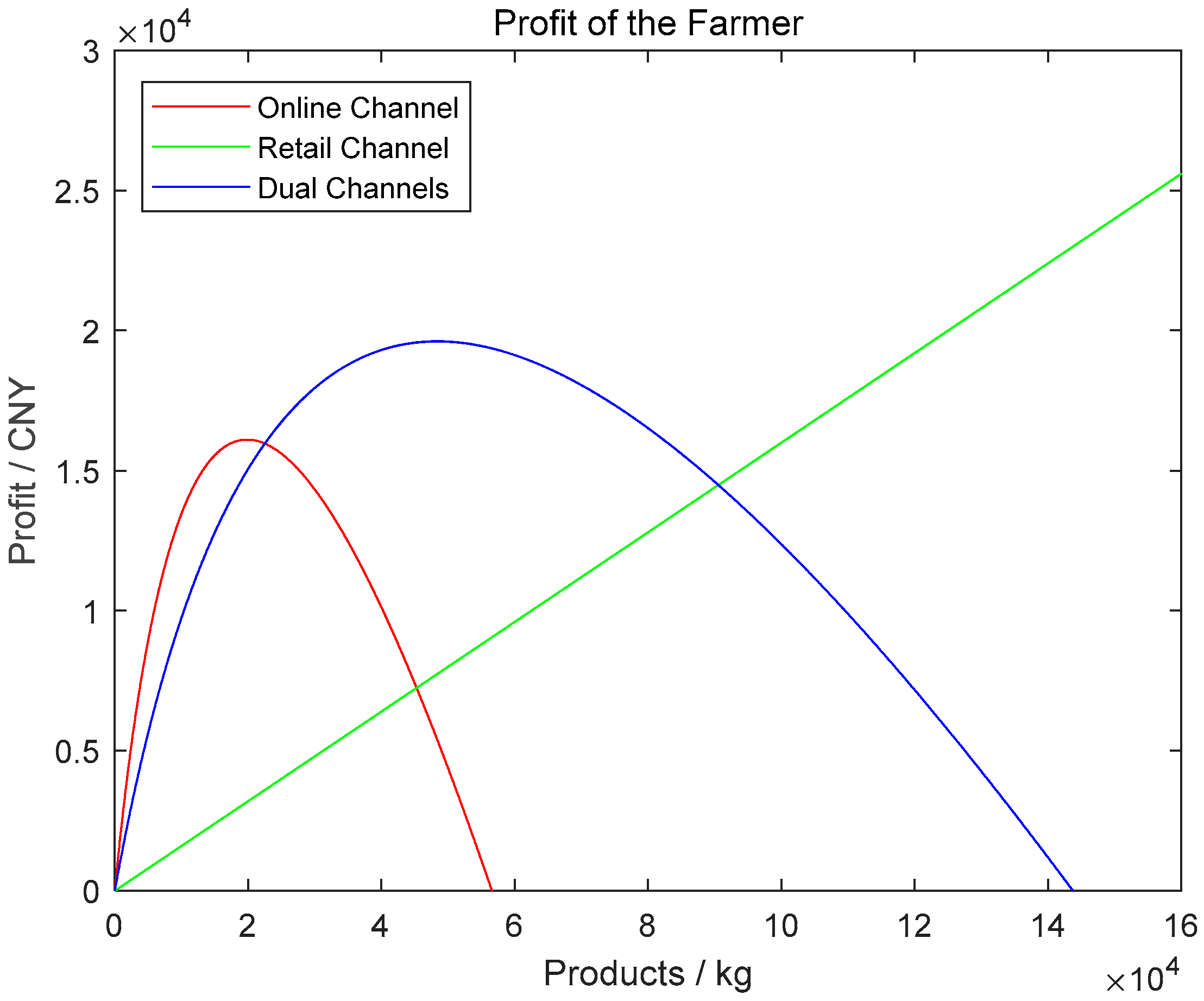
Based on this,
Figure 3 is plotted to show how profit function changes as yield grows, which proves Lemma 1 and provides an optimal profit channel selection strategy as Theorem 1. In
Figure 3, with the fixed
, we use letters X, Y, Z to represent three intersection points where we set the yield values of three intersection points satisfy the following inequation:
. When the actual yield of the farmer is less than
(
), selecting the online channel would bring optimal profit. When the yield of the farmer is between
and
(
), choosing dual channels would bring more profit, and when the yield
is more than
(
), the adoption of the retail channel would create the most profit. Because the scale effects have not formed when the yield is low, higher unit price is the reason for getting more profit through the online channel. When the yield is high, production is oversupplied in the online channel because of the finite constant demand rate. However, contracts between the farmer and the retailer are signed in the retail channel, which enables the farmer to sell more with less risk. Thus, the retail channel is the optimal channel when the yield is high, and the online channel is appropriate for low yield. Otherwise, the dual channels are optimal.
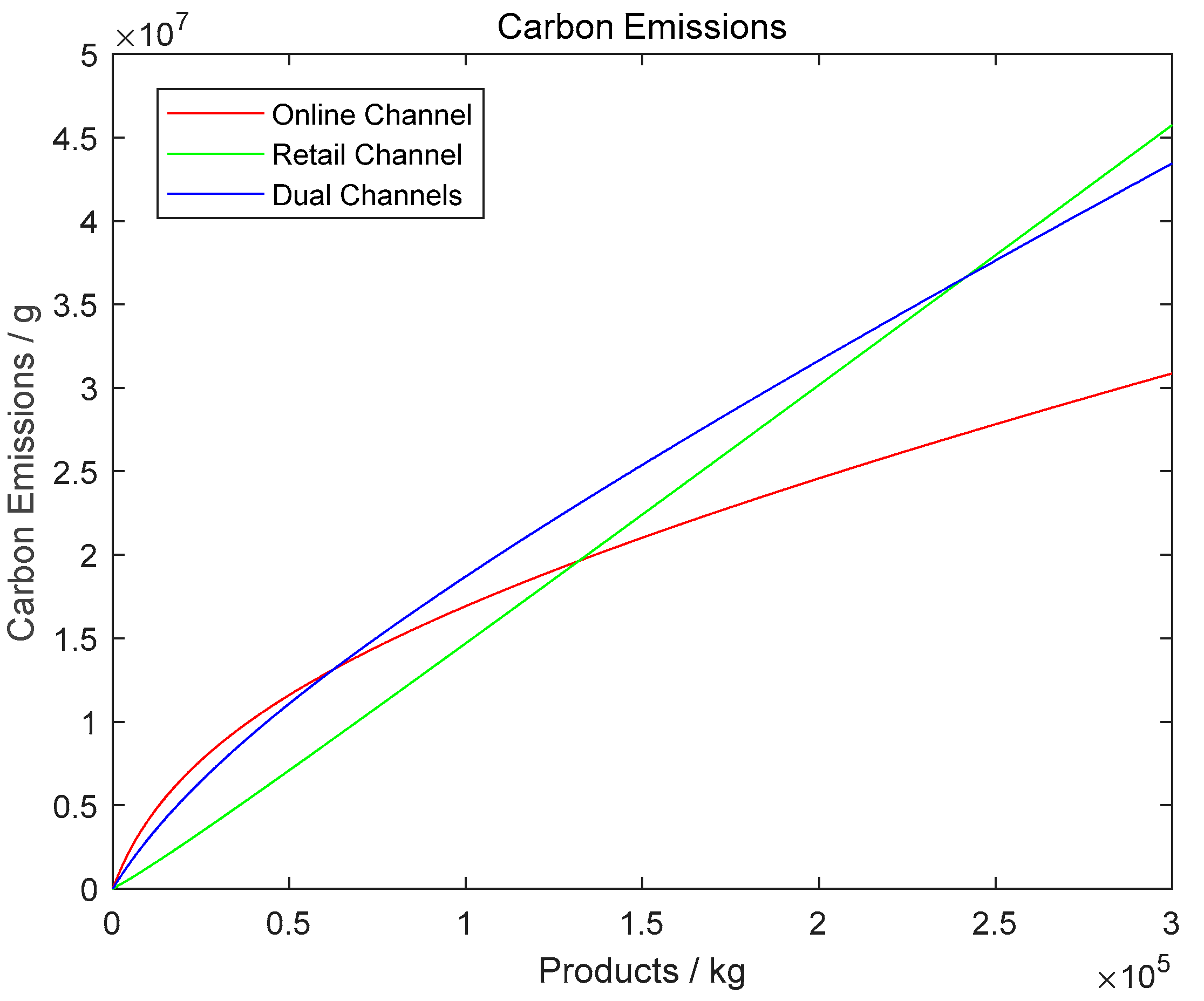
To analyze how carbon emissions of three channels change as yield grows, we observe three channels’ emissions correlations in
Figure 4. It proves the optimal emission channel selection strategies as Theorem 4. In
Figure 4, we also use letters A, B, C to represent three intersection points where we set the yield values of three intersection points satisfy the following inequation:
. When the yield value is less than
(
) the retail channel will produce the least carbon emissions. When the yield is more than
(
), choosing the online channel produces fewer carbon emissions. The quantity of transported products is different between two single channels, thus the unit carbon emissions of transporting is quite different as well. The online channel transporting tends to have more mileage compared with the retail channel. Generally speaking, unit transporting emissions of the online channel are more than those of the retail channel. Thus, when the yield is at a low level, higher transporting emissions of the online channel are the main reason that carbon emissions of the retail channel are low. When the yield is at a high level, deterioration happens in the online channel, thus the quantity of products transported in the online channel is much lower than that in the retail channel, which results in carbon emissions of the online channel being lower.
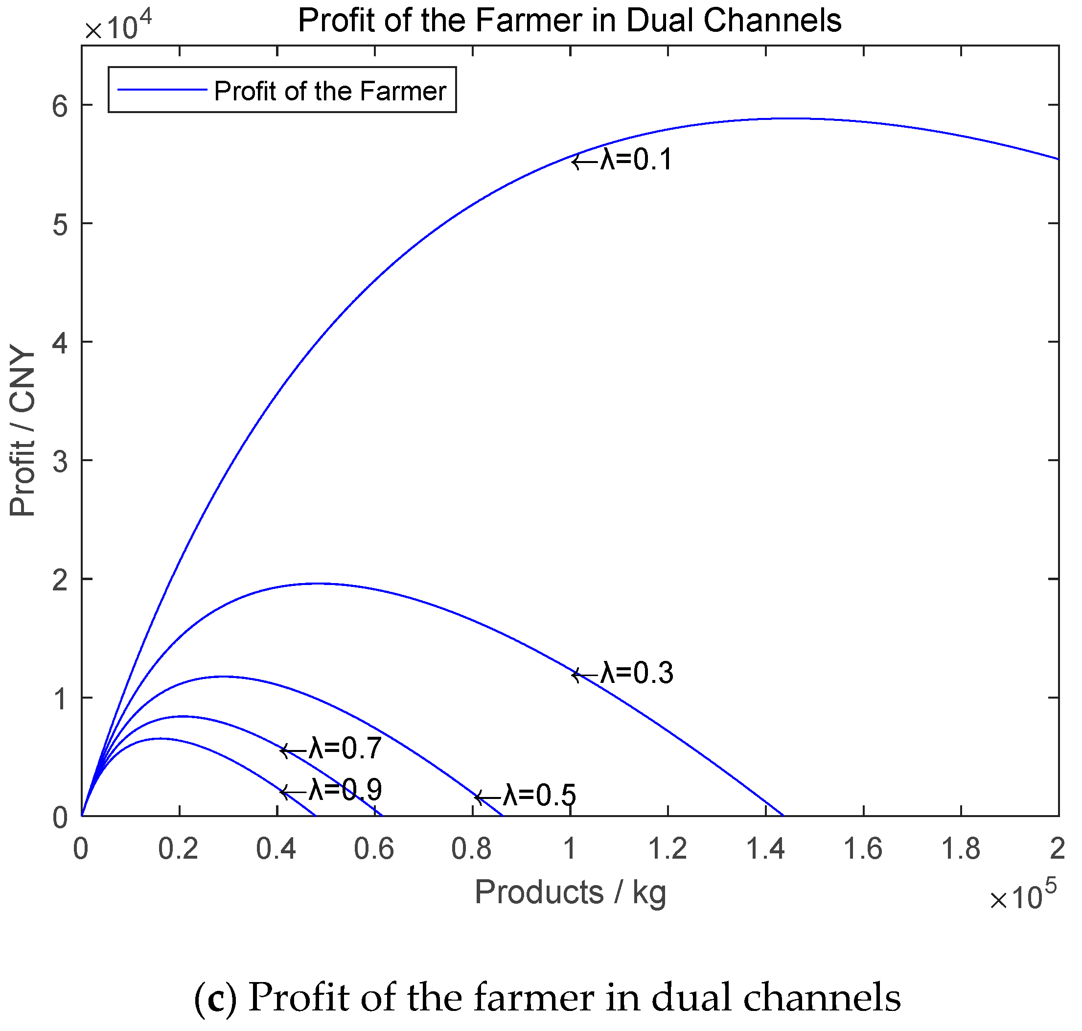
5.1. The Impact of the Deterioration Rate () on Profit
We take 200,000 as the limitation of the yield to show the effects of deterioration rate on the channel profits and the channel decisions. Based on the below analysis, we can obtain further insights about the correlation between the deterioration rate and different channels.
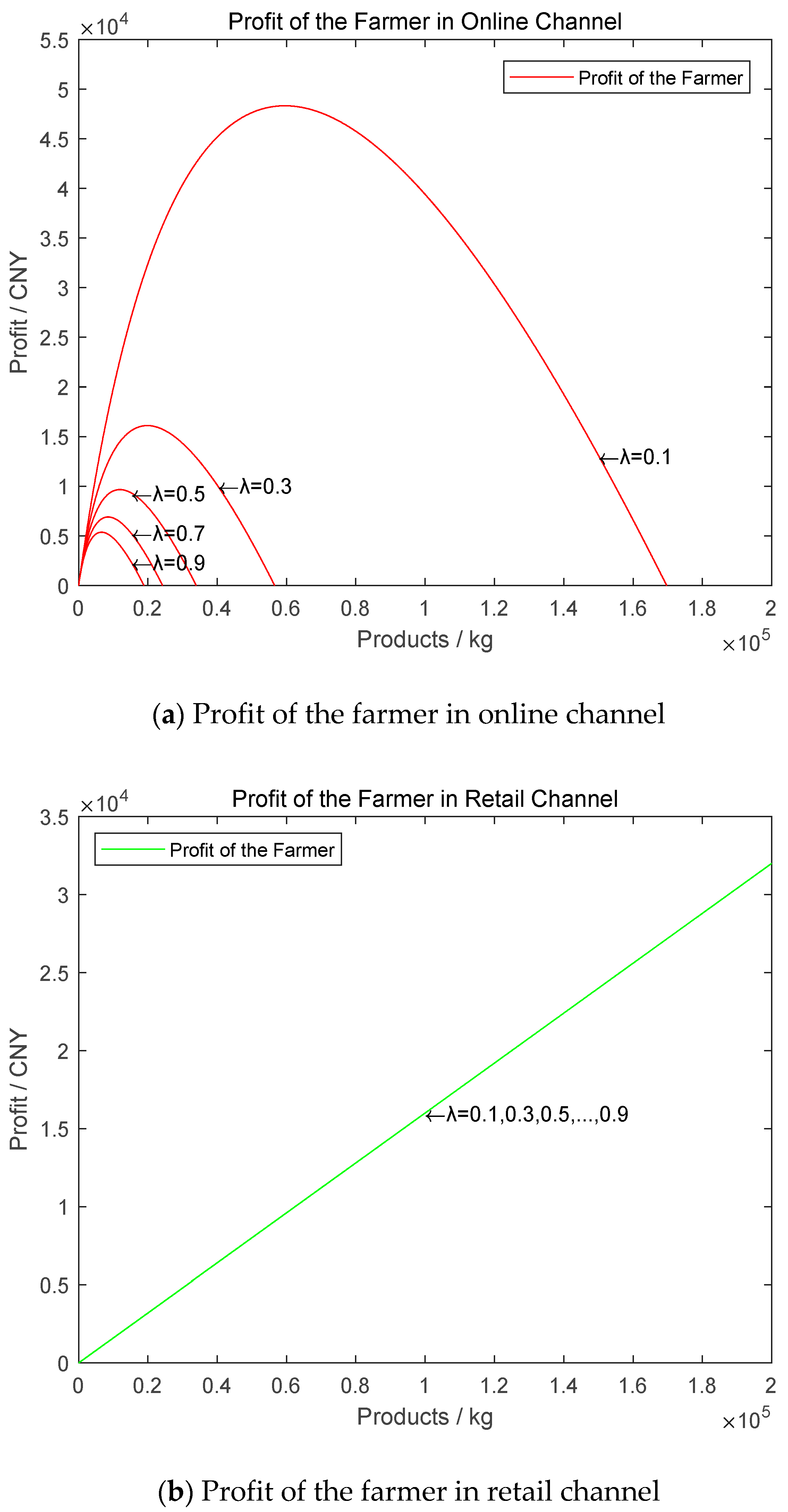
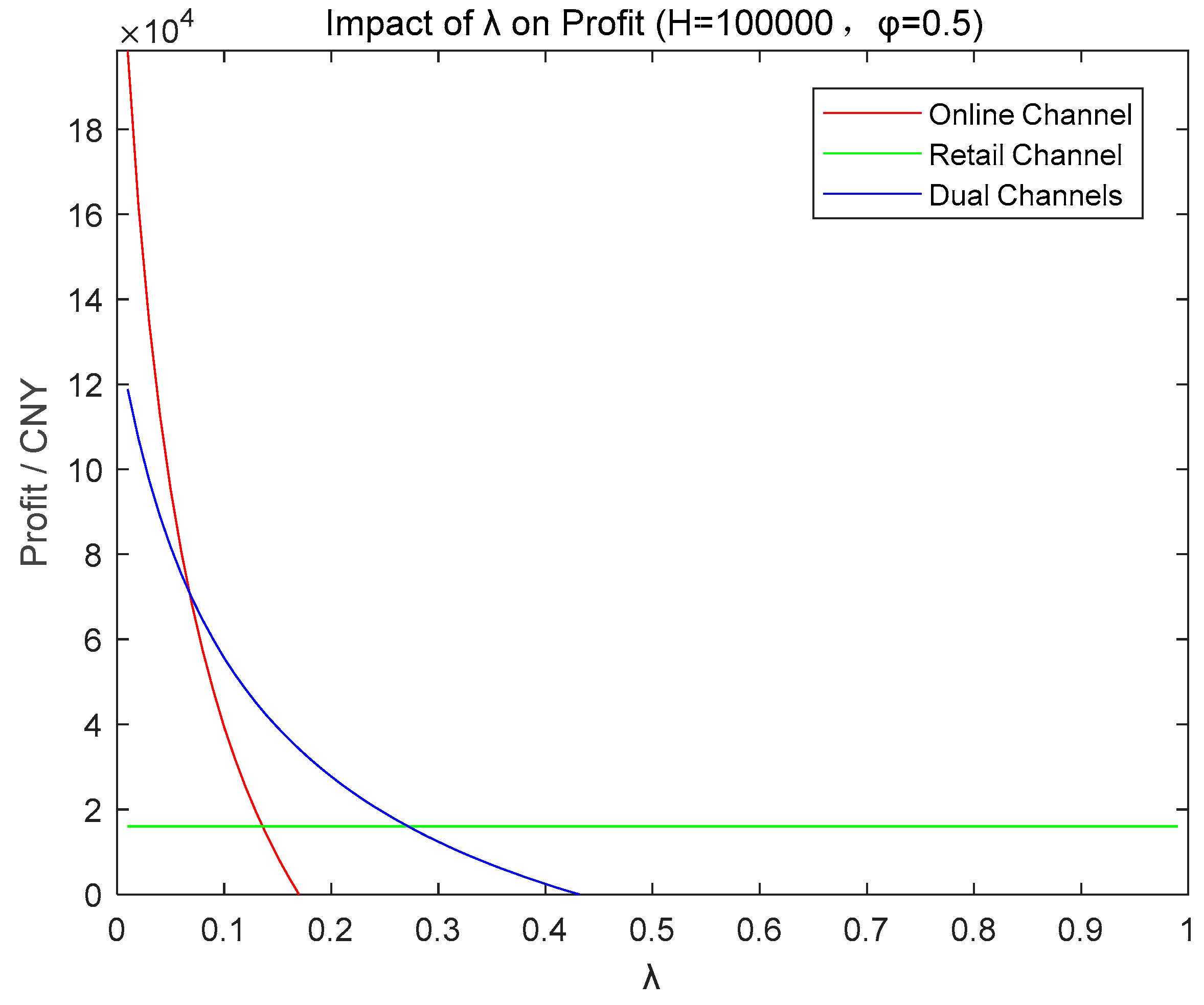
Firstly,
Figure 5 shows us the profit changes with the deterioration rate varying in three different channels. The insights we can gain include: (1) profit of the retail channel is not sensitive as the deterioration rate changes. This is due to the contract that the farmer signs with the retailer in advance, which ensures the reliability and the security of sales in the retail channel. Almost all kinds of products are suitable for the retail channel; (2) profit of the online channel is sensitive to the change of the deterioration rate. The lower the deterioration rate is, the higher the profit will be at the same yield. Meanwhile, compared to a low deterioration rate, when the deterioration rate is high, the farmer’s profit will become negative at the relatively low level of yield, which indicates products with a high deterioration rate are not suitable for the online channel; (3) similar to the online channel, the profit of the dual channels is sensitive to the deterioration rate, but it is less sensitive than the online channel, which means more products can be accepted in the dual channels.
Then, we compare the three channels’ profits and find that the retail channel’s profit is always positive in relation to the yield. However, the optimal yield exists in both the online channel and the dual channels. For the same product, the dual channels’ optimal yield is higher than the optimal one in the online channel. This result could motivate the farmer to exploit new sales channels to get the potential profit from the new channel.
To be specific, we give an example with a certain yield and illustrate how profit changes when the deterioration rate grows in
Figure 6. We can verify that profit in the retail channel has the lowest sensitivity, which is displayed as a straight line parallel with the
X-axis. Profit in the online channel has the highest sensitivity. There are three points of intersection named X, Y, Z, and the deterioration rate of three points are set as
,
,
with the inequation
satisfied. It shows that when a product’s deterioration rate
is less than
(
), selecting the online channel enables the farmer to get highest profit. When the deterioration rate is between
and
(
), choosing the dual channels would be the optimal. Otherwise (
), the retail channel is the best choice.
Overall, through the above analysis, the farmer’s channel decisions should take the yield and the deterioration rate into account. Different types of products have different optimal sales channels. Moreover, the farmer can exploit new sales channels to get more market and profit. These results provide theoretical foundation for the channel selection.
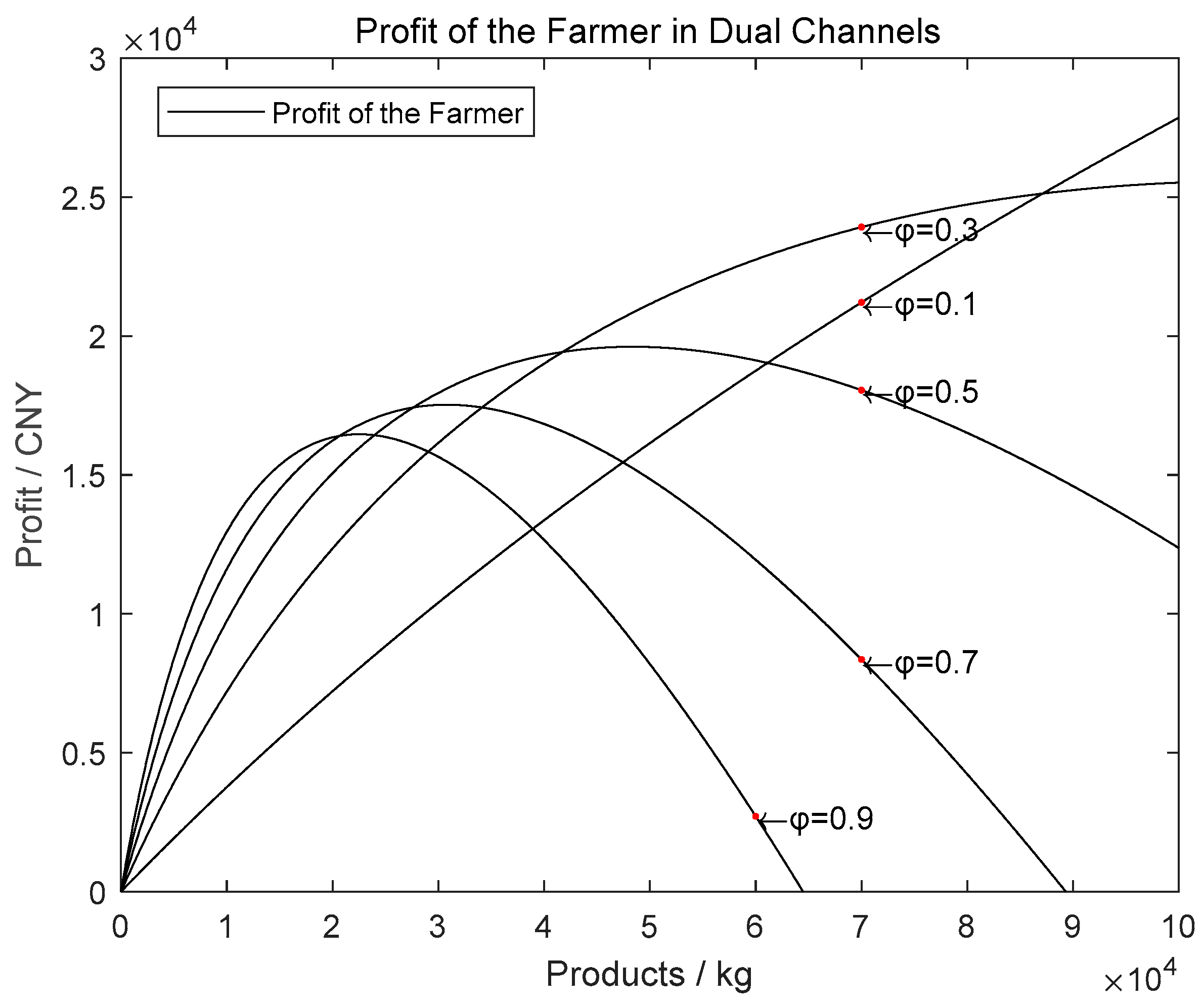
5.2. The Impact of Proportion of Products Sold Online on Profit
In this part, we discuss further insights considering the impact of online sales proportion on profit. To discuss the impact on profit when the proportion varies, we change it from
to
in the step of
and then show this in
Figure 7.
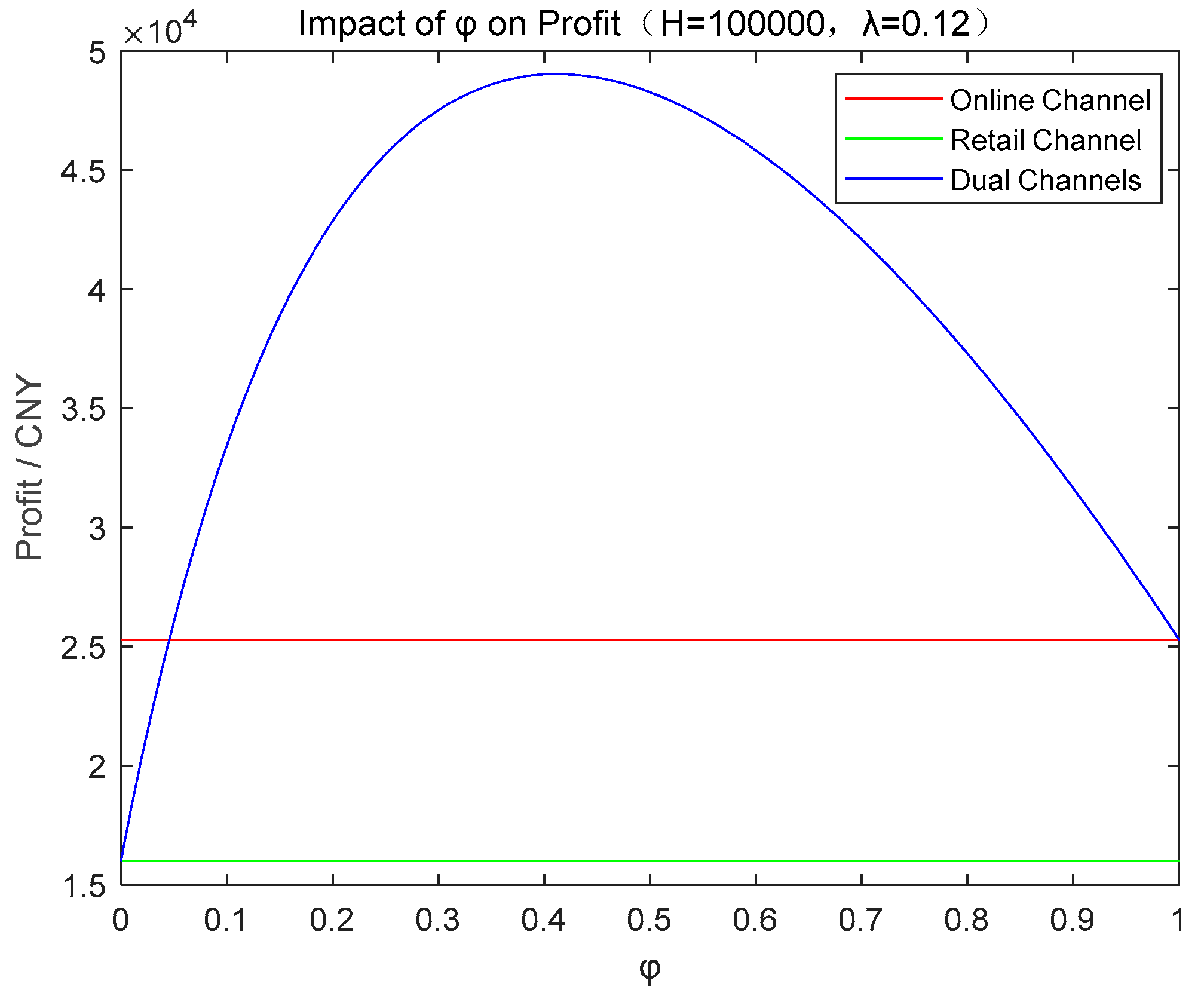
Firstly, we find that the optimal online sales proportion always exists for certain yield in dual channels, which proves the analysis above.
Figure 8 shows how profit in three channels will change as proportion grows when the yield is
and the deterioration rate is 0.12. Dual channels are sensitive to the proportion, but single channels are not. There also exists an optimal proportion. Thus, if the farmers can ensure their producing plans in next year, this is the guideline for them to allocate the products selling in different channels. With the same reason, each proportion has a respective optimal yield, which also offers suggestions to the farmer. The farmers’ producing decisions are related to each other. Additionally, as the yield grows, the optimal profit happens at a lower proportion. On the contrary, when the yield is low, more products would be sold online. Higher unit price can bring more profit for the farmer when yield is low. However, the scale effect would take much more profit in the retail channel compared to the online channel when the yield is high.
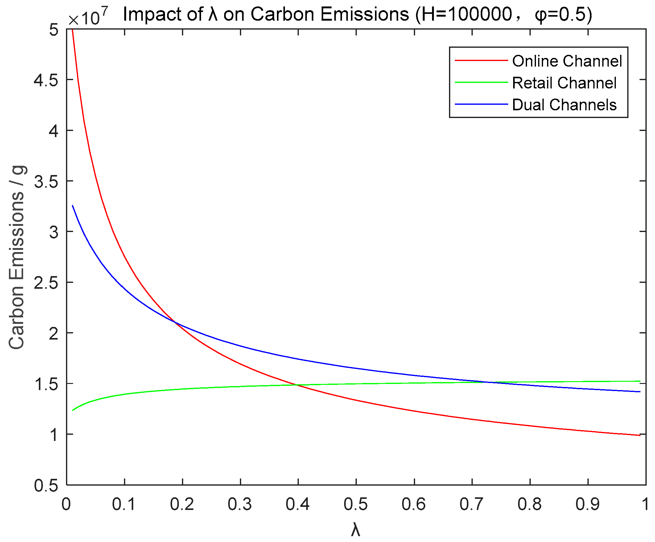
5.3. The Impact of the Deterioration Rate on Carbon Emissions
To discuss how carbon emissions change when the deterioration rate changes, we show the functions below with a certain yield.
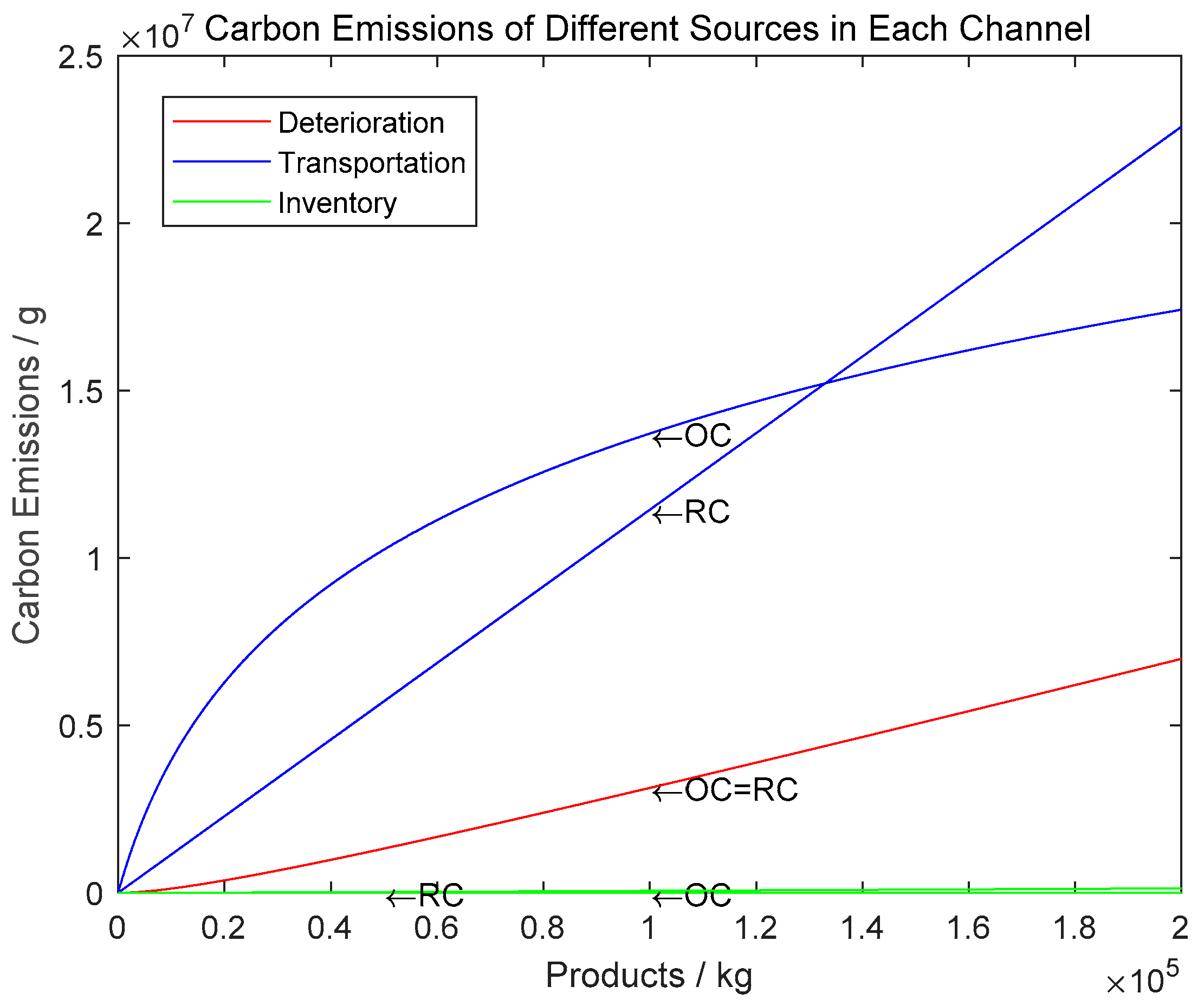
Figure 9,
Figure 10 and
Figure 11 convey several results: (1) the carbon emissions in the online channel are the most sensitive to the deterioration rate, while the retail channel is the least sensitive one. The correlation between carbon emissions and deterioration rate is positive in the retail channel, while it is negative in both the online channel and the dual channels. With the deterioration rate increasing, more deterioration will happen online, which means fewer products will be transported and fewer carbon emissions will be used in the online channel. The same tendency can be concluded in the dual channels. However, for the retail channel, although more deterioration happens in the retailer, when the deterioration rate is higher, the number of products delivered from the farmer to the retailer does not decrease; (2) the difference of carbon emissions among the three channels mainly depends on the transporting emissions online and offline. As analyzed above, when the deterioration rate is low, the difference of the transported products quantity between two single channels is not large. In this situation, the online channel will produce more carbon emissions because of the high-carbon transporting process. However, the products transported in the retail channel are much more than that in the online channel when the deterioration rate is high. The retail channel generates more carbon emissions than the online channel does, thus the difference is mainly from the delivering process in which the carbon emissions mainly depend on the transported quantity and the distance; (3) when the deterioration rate is low, the amount of deterioration increases rapidly, and with an increase of the deterioration rate, the increasing slows down when the rate is high. Thus, to control the deterioration, the farmer and the retailer can invest in warehouses to maintain a low deterioration rate.
From the above, we know that the farmers can adjust their operations to get the optimal profit. Farmers can choose the sales channel within the consideration of yield and deterioration rate. The farmer can also exploit the new channel to enlarge the market. High deterioration products are not suitable for online selling. Thus, the farmer can choose the channel according to the type of product. At the same time, it is beneficial to carry the carbon tax policy to control the emissions for governments; the farmer can also promote the use of some low-carbon transporters—such as electric vehicles—to restrain the emissions. Additionally, the investment in the cold chain is also important to control the deterioration, which could reduce the waste and also meet the market demand with less production.
6. Conclusions and Future Research
The contributions of this paper are mainly embodied in the following two points. Firstly, the channel selection based on the maximum profit and the minimum carbon emissions are obtained. Then, the impact of the deterioration rate and the proportion of online sales on channel profits and carbon emissions are analyzed through the systematical channel comparison and sensitivity analysis. They prove the theoretical basis for farmers and the government to make decisions, which is beneficial for the country’s economy development and environmental protection.
This paper is mainly about the discussion on the farmer’s channel selection. There are three types of sales channels: online, retail, and dual channels. At the same time, it also considers the influence of low-carbon policies on the retailer of the supply chain, which leads to an impact of the farmer’s decision-making. In addition, we conducted sensitivity analysis of the channel sales profit and the channel carbon emissions on the decay rate of agricultural products and the proportion of online sales. Here, we present some broad conclusions.
For the farmer, first, there exists a most profitable channel for fixed output, but it may conflict with the optimal sales channel with the aim of lower carbon emissions. Second, after adopting a carbon tax, the sales cycle of the retailer in the supply chain will be shortened, and the farmer’s offline sales will be reduced, which will have a great impact on the offline sales and dual-channel sales. At the same time, the proportion of online sales will increase. Third, the retail channel can be adopted for products with high deterioration, while the online channel is not applicable for products with high deterioration. Moreover, the online channel’s profit is more sensitive to the deterioration rate when the rate is low. Finally, if more products are sold online, then the farmer’s optimal yield is lower. Thus, for the farmer, a reasonable distribution of their online sales proportion will result in higher profits, and the farmers can maximize profits by selecting their own scientific management and sales channels for production and sales. At the same time, the farmer should take some measures to keep the deterioration rate at a low level.
For governments, first, the carbon tax has less impact on the farmer than the retailer, and the total carbon emissions will decrease after carrying out the carbon tax. Second, the difference of carbon emissions between two single channels mainly comes from the transportation and the inventory process. Thus, governments can encourage companies to increase their anti-corrosion measures and investments in cold chain logistics to help the farmer achieve higher profits. In order to protect the environment and control the total amount of carbon emissions, governments should gradually impose carbon emissions costs on related enterprises in the agricultural products industry and carry out relevant subsidies to guide the farmer to choose the environmental channel. Moreover, governments should improve the transportation process, such as the overall planning of goods or the promotion of electric logistics vehicles.
At the same time, there are some limitations in this paper. First, the calculation of the carbon footprint is simplified in this paper, which has a certain deviation from the actual situation. Second, there are more carbon sources than the sources we mentioned and calculated in the paper, such as the inventory carbon emissions from logistics transfer stations, carbon emissions from equipment in the cold chain, and so on. In addition, this paper also omits some other channels that the farmer can choose. For example, the farmer sells in the third-party platform online, and then the platform sells to consumers, and so on. These simplifications prevent this paper from analyzing more possible scenarios, but they also provide a direction for future low-carbon agricultural product research.
Author Contributions
Writing, C.Z., Q.P.; Providing case and idea, Q.P., C.Z., G.W., T.L., Y.C. and L.Y.; Formal analysis, Q.P and. C.Z.; Supervision, Y.C. and L.Y.; Revising draft Q.P., C.Z., G.W., T.L, Y.C. and L.Y.
Funding
This work is supported by the National Nature Science Foundation of China (Grant No. 71572058), National Training Program of Innovation and Entrepreneurship for Undergraduates 2018, Soft Science Program of Guangdong Province (Grant No. 2018A070712002), and the Fundamental Research Funds for the Central Universities Foundation of China (Grant No. 2018ZDXM05).
Conflicts of Interest
The authors declare no conflict of interest.
Appendix A
Appendix A.1. Objective Function and Decision Variables of the Farmer and the Retailer without the Carbon Tax
(1) In scenario R, we discuss the retailer’s decision first according to the Stackelberg model. With the inventory model given by Ghare et al, by setting the inventory level to zero at the end of a sales period as the boundary condition, we can get the inventory function of the retailer as follows: . Thus, the quantity of order is and the profit of the farmer could be described as follows: . The profit of the retailer could be described as . To get the optimal sales period of the retailer, we take the partial of with respect of and we get the optimal . The yield of the farmer is limited by the order and could be described as . To do the calculation of the carbon emissions of the entire supply chain, we determine that the emissions come from three parts, which are deterioration, transportation, and inventory. In the scenario R, for the quantity of products deteriorated, we get the equation . For the part of transportation, we get the expression . For the part of inventory, we get the expression . According to assumption (6), we can determine that the carbon emissions of the retail channel is .
(2) In scenario O, by setting inventory level at the beginning of a sales period as the boundary condition, we can get the inventory function of the farmer as . Thus, we can get the profit function of the farmer as follows: . To get the optimal yield , we take the partial of with the respect of and we get the optimal . For the quantity of products deteriorated, we get the equation . For the part of transportation, we get the expression . For the part of inventory, we get the equation . Therefore, we can get the carbon emissions in the online channel as .
(3) In scenario D, we simply substitute the into the of the farmer’s profit function in scenario O and into the of the farmer’s profit function in scenario R. Therefore, we can get the profit function of the farmer as . Because the Stackelberg still fits the situation, the retailer’s decision is discussed first, and the optimal remains unchanged. For the farmer, as the constraint is , the yield of the farmer depends on the retailer’s decisions. For the farmer, the proportion of products sold online is what he can decide. To get the optimal , we take the partial of with respect of after substituting the expression of into the function. We get the optimal proportion . For the carbon emissions in dual channels, we replace the of the carbon emission expression in the retail channel and replace the of the carbon emission expression in the online channel with . Thus, we can get the carbon emissions in the dual channels as .
Appendix A.2. Objective Function and Decision Variables of Farmer and Retailer with the Carbon Tax
As the carbon tax is only imposed on the retailer in the retail channel and the dual channels, the farmer’s profit functions remain unchanged. The retailer is supposed to be responsible for the emissions made by them. The impact of carbon tax on the supply chain works in the approach of affecting the retailer’s decisions. Thus, the retailer’s profit function changes into an expression as . With the change of retailer’s profit function, we take the partial of with the respect of , and the optimal changes into a new value .
Appendix B
Proof of Lemma 1. To get the optimal in the online channel, we take the partial of with respect to : . Setting it as , we can get the extreme point. After verification, we have if and if . □
Proof of Theorem 1. Existence of the intersection points will be proved here. We create a function , and now the problem is transformed to prove that the function has zeros. We take the partial of with respect to , which is . Setting , we get the equation . When , has one extreme point at ’s interval . has a limitation and an equation , which indicates that the extreme point is the extreme large point. In this case, there is one intersection point between and . Then, the existence of the intersection between and will be proved in the same way. We create a function . To prove that the has zeros, we take partial of it with respect to , which is , increasing when is growing. Setting , we can get . Therefore, will initially decrease but begin to increase after reaching the extremely small point . Because and , there is certainly one zero when grows from , which means that and have one intersection point. At last, we prove the existence of the intersection point between and in the same way. We create a new function first, and then take partial of it with respect to , which is . It increases as grows. Setting , and we can get , which indicates that will initially decrease but turn to increase after reaching the extremely small point . Because , there is certainly one zero when grows from which means that and have one intersection point. □
Proof of Theorem 2. The farmer’s profit function in the online channel is . We take the partial of with respect to , which is . The farmer’s profit function in the retail channel is . We take the partial of with respect to , which is . The farmer’s profit function in the dual channel is . Because of the constraint , with substituting it into , we take the partial of with respect to , which is . □
Proof of Lemma 2. , . To prove is to prove . By transposition, we can get the inequation to prove , . □
Proof of Lemma 3. The function describing carbon emissions in the retail channel is . We take the partial of it with respect to , which is , indicating that the partial decreases as grows. Setting , we get the extreme point , thus when , is satisfied always. With the same approach, we can verify that . If , and then the inequation is demanded, which is contrasted with the constraint . Thus, is satisfied always. □
Proof of Theorem 4. Existence of the intersection points will be proved. Firstly, for two single channels, we create a function . Now the task is transformed to prove the function has zeros. We take the partial of with respect to , which is . Setting , we get the equation . When , we can solve the inequation to get the limitation of H, . We also have , , thus there exists an extreme small point and a null point of function , respectively, which indicates the intersection point of two single channels’ carbon emission function curves exists. □
Proof of Theorem 5. The carbon emissions’ equation in the online channel is . We take the partial of it with respect to . The carbon emissions’ equation in the retail channel is . Because of the constraint , with the constraint substituted into the equation, we get . After taking the partial of it with respect to , we can get . Thus, when , we have . Obviously, with the restriction that all parameters are positive, is satisfied when . It could be also proved that is satisfied when . In the online channel, as the retailer is not a supply chain member, has no influence on the carbon emissions. □
References
- National Bureau of Statistics of China. Rural Population in 2018; National Bureau of Statistics of China: Beijing, China, 2018. Available online: http://data.stats.gov.cn/easyquery.htm?cn=C01 (accessed on 10 January 2018).
- National Bureau of Statistics of China. Per-Capita Disposable Income of Urban Households and Per-Capita Net Income of Rural Households; National Bureau of Statistics of China: Beijing, China, 2018. Available online: http://data.stats.gov.cn/easyquery.htm?cn=C01 (accessed on 10 January 2018).
- National Bureau of Statistics of China. Average Net Income Per Capital of Rural Household; National Bureau of Statistics of China: Beijing, China, 2017. Available online: http://www.stats.gov.cn/ (accessed on 10 January 2018).
- Zhang, Q.Q.; Yan, B.B.; Huo, X.X. What are the Effects of Participation in Production Outsourcing? Evidence from Chinese Apple Farmers. Sustainability 2018, 10, 4525. [Google Scholar] [CrossRef]
- Liu, H.Y.; Zhang, J.L.; Zhou, C.; Ru, Y.H. Optimal Purchase and Inventory Retrieval Policies for Perishable Seasonal Agricultural Products. Omega 2017, 79, 133–145. [Google Scholar] [CrossRef]
- The Xinhua News Agency. Ten Thousand Pounds of Pitaya Unmarketable Fish into the Pond to Feed the Fish in Guangdong Foshan; The Xinhua News Agency: Beijing, China, 2015; Available online: https://new.qq.com/cmsn/20150703/20150703028097 (accessed on 7 March 2015).
- Malekitabar, M.; Yaghoubi, S.; Reza, M. A Novel Mathematical Inventory Model for Growing-mortal Items (Case Study: Rainbow Trout). Appl. Math. Model. 2019, 71, 96–117. [Google Scholar] [CrossRef]
- China State Council. The State Council Issued a Notice on the 13th Five-Year Plan for Poverty Alleviation; China State Council: Beijing, China, 2016. Available online: http://www.gov.cn/zhengce/content/2016-12/02/content_5142197.htm (accessed on 23 November 2016).
- Al-Mansour, F.; Jejcic, V. A Model Calculation of the Carbon Footprint of Agricultural Products: The Case of Slovenia. Energy 2017, 136, 7–15. [Google Scholar] [CrossRef]
- Yang, L.; Ji, J.N.; Wang, M.Z.; Wang, Z.Z. The Manufacturer’s Joint Decisions of Channel Selections and Carbon Emission Reductions Under the Cap-and-trade Regulation. J. Clean. Prod. 2018, 193, 506–523. [Google Scholar] [CrossRef]
- Baranzini, A.; Goldemberg, J.; Speck, S. A Future for Carbon Taxes. Ecol. Econ. 2000, 32, 395–412. [Google Scholar] [CrossRef]
- China Leads the World in Terms of Carbon Emissions. Chinese Carbon Trading Website. 2017. Available online: http://www.tanjiaoyi.com/article-23347-1.html (accessed on 10 December 2017).
- People’s Daily. China May Introduce a Carbon Tax After 2020; People’s Daily: Beijing, China, 2016; Available online: http://www.tanpaifang.com/tanshui/2016/0810/55358.html (accessed on 10 August 2016).
- Benjaafar, S.; Li, Y.; Daskin, M. Carbon Footprint and the Management of Supply Chains: Insights from Simple Models. IEEE Trans. Autom. Sci. Eng. 2013, 10, 99–116. [Google Scholar] [CrossRef]
- Strutt, J.; Wilson, S.; Shorney, D.H. Assessing the Carbon Footprint of Water Production. J. Am. Water Works Assoc. 2008, 100, 80–89. [Google Scholar] [CrossRef]
- Cappelletti, G.M.; Nicoletti, G.M.; Russo, C. Life Cycle Assessment (LCA) of Spanish-style Green Table Olives. Ital. J. Food Sci. 2010, 22, 3–14. [Google Scholar]
- Jensen, J.K.; Arlbjorn, J.S. Product Carbon Footprint of Rye Bread. J. Clean. Prod. 2014, 82, 45–47. [Google Scholar] [CrossRef]
- Wang, Q.; Zhao, D.; He, L. Contracting Emission Reduction for Supply Chains Considering Market Low-carbon Preference. J. Clean. Prod. 2016, 120, 72–84. [Google Scholar] [CrossRef]
- Krass, D.; Nedorezov, T.; Ovchinnikov, A. Environmental Taxes and The Choice of Green Technology. Hist. J. Film Radio 2011, 22, 1035–1055. [Google Scholar] [CrossRef]
- Ji, J.N.; Zhang, Z.Y.; Yang, L. Carbon Emission Reduction Decisions in the Retail Dual-channel Supply Chain with Consumers’ preference. J. Clean. Prod. 2017, 141, 852–867. [Google Scholar] [CrossRef]
- Martin, R.; De Preux, L.B.; Wagner, U.J. The Impact of a Carbon Tax on Manufacturing: Evidence from Microdata. J. Public Econ. 2014, 117, 1–14. [Google Scholar] [CrossRef]
- Chen, W.T.; Hu, Z.H. Using Evolutionary Game Theory to Study Governments and Manufacturers’ Behavioral Strategies Under Various Carbon Taxes and Subsidies. J. Clean. Prod. 2018, 201, 123–141. [Google Scholar] [CrossRef]
- Wang, C.X.; Wang, W.; Huang, R.B. Supply Chain Enterprise Operations and Government Carbon Tax Decisions Considering Carbon Emissions. J. Clean. Prod. 2017, 152, 271–280. [Google Scholar] [CrossRef]
- Xu, C.Y.; Gou, Q.L. Pricing Issues in a Two-echelon Dual-channel Supply Chain. Syst. Eng. Theory Pract. 2010, 30, 1741–1752. [Google Scholar]
- Suh, S.; Huppes, G. Methods for Life Cycle Inventory of a Product. J. Clean Prod. 2005, 13, 687–697. [Google Scholar] [CrossRef]
- Chojnacka, K.; Kowalski, Z.; Kulczycka, J. Carbon Footprint of Fertilizer Technologies. J. Environ. Manag. 2019, 231, 962–967. [Google Scholar] [CrossRef]
- Yan, M.; Cheng, K.; Luo, T.; Yan, Y.; Pan, G.X. Carbon Footprint of Grain Crop Production in China—Based on Farm Survey Data. J. Clean. Prod. 2015, 104, 130–138. [Google Scholar] [CrossRef]
- Zhang, W.S.; He, X.M.; Zhang, Z.D.; Gong, S. Carbon Footprint Assessment for Irrigated and Rainfed Maize (Zea Mays L.) Production on the Loess Plateau of China. Biosyst. Eng. 2018, 167, 75–86. [Google Scholar] [CrossRef]
- Carrillo, J.E.; Vakharia, A.J.; Wang, R. Environmental Implications for Online Retailing. Eur. J. Oper. Res. 2014, 239, 744–755. [Google Scholar] [CrossRef]
- Hua, G.W.; Cheng, T.C.E.; Wang, S.Y. Managing Carbon Footprints in Inventory Management. Int. J. Prod. Econ. 2011, 132, 178–185. [Google Scholar] [CrossRef]
- Tsai, W.-H. A Green Quality Management Decision Model with Carbon Tax and Capacity Expansion Under Activity-Based Costing (ABC)—A Case Study in the Tire Manufacturing Industry. Energies 2018, 11, 1858. [Google Scholar] [CrossRef]
- Yang, L.; Chen, M.; Cai, Y.J.; Tsai, S.B. Manufacturer’s Decision as Consumers’ Low-Carbon Preference Grows. Sustainability 2018, 10, 1284. [Google Scholar] [CrossRef]
- Fruchter, G.E.; Tapiero, C.S. Dynamic Online and Offline Channel Pricing for Heterogeneous Customers in Virtual Acceptance. Int. Game Theory Rev. 2005, 7, 137–150. [Google Scholar] [CrossRef]
- Khouja, M.; Park, S. Channel Selection and Pricing in the Presence of Retail-captive Consumers. Int. J. Prod. Econ. 2010, 125, 84–95. [Google Scholar] [CrossRef]
- Chiang, W.K.; Chhajed, D.; James, D.H. Direct Marketing, Indirect Profits: A Strategic Analysis of Dual-channel Supply Chain Design. Manag. Sci. 2003, 49, 1–20. [Google Scholar] [CrossRef]
- Wang, W.; Li, G. Channel Selection in a Supply Chain with a Multi-channel Retailer: The Role of Channel Operation Costs. Int. J. Prod. Econ. 2016, 173, 54–65. [Google Scholar] [CrossRef]
- Yang, L.; Tang, R.H. Comparisons of Sales Modes for a Fresh Product Supply Chain with Freshness-keeping Effort. Transp. Res. Part E Logist. Transp. Rev. 2019, 125, 425–448. [Google Scholar] [CrossRef]
- Abdelsalam. A Simulation Model for Managing Marketing Multi-Channel Conflict. Int. J. Syst. Dyn. Appl. 2015, 1, 59–76. [Google Scholar]
- Hao, J.H.; Bijman, J.; Gardebroek, C. Cooperative Membership and Farmers’ choice of Marketing Channels—Evidence from Apple Farmers in Shaanxi and Shandong Provinces, China. Food Policy 2018, 74, 53–64. [Google Scholar] [CrossRef]
- Negi, D.S.; Birthal, P.S.; Roy, D.; Khan, M.T. Farmers’ choice of Market Channels and Producer Prices in India: Role of Transportation and Communication Networks. Food Policy 2018, 81, 106–121. [Google Scholar]
- Blackburn, J.; Scudder, G. Supply Chain Strategies for Perishable Products: The Case of Fresh Produce. Prod. Oper. Manag. 2009, 18, 129–137. [Google Scholar] [CrossRef]
- Bakker, M.; Riezebos, J.; Teunter, R.H. Review of Inventory Systems with Deterioration Since 2001. Eur. J. Oper. Manag. 2012, 221, 275–284. [Google Scholar] [CrossRef]
- Janssen, L.; Claus, T.; Sauer, J. Literature Review of Deteriorating Inventory Models by Key Topics From 2012 to 2015. Int. J. Prod. Econ. 2016, 182, 86–112. [Google Scholar] [CrossRef]
- Tiwari, S.; Chandra, K.J.; Gupta, M.; Eduardo, L. Optimal Pricing and Lot-sizing Policy for Supply Chain System with Deteriorating Items under Limited Storage Capacity. Int. J. Prod. Econ. 2018, 200, 278–290. [Google Scholar] [CrossRef]
- Sarkar, B.; Sarkar, S. Variable Deterioration and Demand—An Inventory Model. Ecol. Model. 2013, 31, 548–556. [Google Scholar] [CrossRef]
- Qin, Y.Y.; Wang, J.J.; Wei, C.M. Joint Pricing and Inventory Control for Fresh Produce and Foods with Quality and Physical Quantity Deteriorating Simultaneously. Int. J. Prod. Econ. 2014, 152, 42–48. [Google Scholar] [CrossRef]
- Giri, B.C.; Chaudhuri, K.S. Deterministic Models of Perishable Inventory with Stock-dependent Demand Rate and Nonlinear Holding Cost. Eur. J. Oper. Res. 1998, 105, 467–474. [Google Scholar] [CrossRef]
- Ghare, P.M.; Schrader, G.P. A Model for Exponentially Decaying Inventory. J. Ind. Eng. 1963, 14, 238–243. [Google Scholar]
Figure 1.
Scenario R, O, D.
Figure 1.
Scenario R, O, D.
Figure 2.
Model comparison and analysis method diagram.
Figure 2.
Model comparison and analysis method diagram.
Figure 3.
Profit functions of farmers in three channels.
Figure 3.
Profit functions of farmers in three channels.
Figure 4.
Carbon emission functions of three channels.
Figure 4.
Carbon emission functions of three channels.
Figure 5.
The impact of the deterioration rate on profit.
Figure 5.
The impact of the deterioration rate on profit.
Figure 6.
Impact of the deterioration rate on profit. (Yield and the proportion of products sold online ).
Figure 6.
Impact of the deterioration rate on profit. (Yield and the proportion of products sold online ).
Figure 7.
Impact of proportion of products sold online on profit.
Figure 7.
Impact of proportion of products sold online on profit.
Figure 8.
Impact of proportion of products sold online on profit. (Yield , and the deterioration ).
Figure 8.
Impact of proportion of products sold online on profit. (Yield , and the deterioration ).
Figure 9.
Impact of the deterioration rate on carbon emissions. (Yield and the proportion of products sold online ).
Figure 9.
Impact of the deterioration rate on carbon emissions. (Yield and the proportion of products sold online ).
Figure 10.
Carbon emissions of different sources in single channel. (Proportion of products sold online ).
Figure 10.
Carbon emissions of different sources in single channel. (Proportion of products sold online ).
Figure 11.
Impact of the deterioration rate on deterioration quantity. (Yield , proportion of products sold online ).
Figure 11.
Impact of the deterioration rate on deterioration quantity. (Yield , proportion of products sold online ).
Table 1.
Notations of parameters and variables.
Table 1.
Notations of parameters and variables.
| Parameters | |
| Wholesale price of the farmer in retail channel |
| The online channel price |
| Selling price of the retailer in retail channel |
| Unit cost of production |
| Unit cost of carbon emissions |
| Unit cost of storage in unit time |
| Deterioration rate of products |
| Demand rate of products |
| Farmer’s duration of selling products online |
| Carbon emissions of unit rotten products |
| Carbon emissions of unit products transported in online channel |
| Carbon emissions of unit products transported in retail channel |
| Carbon emissions of unit products stored in unit time |
| Decision variables | |
| Farmer’s total amount of products |
| Channel selected by farmer |
| Retailer’s duration of selling |
| Retailer’s order quantity |
| Percentage of products sold online |
Table 2.
Profit functions of the farmer and the retailer
Table 2.
Profit functions of the farmer and the retailer
| Scenario | Farmer | Retailer |
|---|
| R | | |
| O | | — |
| D | | |
Table 3.
Decisions without carbon tax.
Table 3.
Decisions without carbon tax.
| Scenario | T2 | φ | H |
|---|
| R | | 0 | |
| O | — | 1 | |
| D | | | |
Table 4.
The farmer’s optimal profit without carbon tax.
Table 4.
The farmer’s optimal profit without carbon tax.
| Scenario | Farmer’s Profit |
|---|
| R | |
| O | |
| D | |
Table 5.
Equations of carbon emissions in channels without carbon tax.
Table 5.
Equations of carbon emissions in channels without carbon tax.
| Scenario | Carbon Emissions |
|---|
| R | |
| O | |
| D | |
Table 6.
Profit functions of the farmer and the retailer
Table 6.
Profit functions of the farmer and the retailer
| Scenario | Farmer | Retailer |
|---|
| R | | |
| O | | — |
| D | |
|
Table 7.
Decisions with carbon tax.
Table 7.
Decisions with carbon tax.
| Scenario | T2 | φ | H |
|---|
| R | | 0 | |
| O | — | 1 | |
| D | | | |
Table 8.
The farmer’s optimal profit without carbon tax.
Table 8.
The farmer’s optimal profit without carbon tax.
| Scenario | Farmer’s Profit |
|---|
| R | |
| O | |
| D |
|
Table 9.
Equations of carbon emissions in channels with carbon tax.
Table 9.
Equations of carbon emissions in channels with carbon tax.
| Scenario | Carbon Emissions |
|---|
| R | |
| O | |
| D | |
© 2019 by the authors. Licensee MDPI, Basel, Switzerland. This article is an open access article distributed under the terms and conditions of the Creative Commons Attribution (CC BY) license (http://creativecommons.org/licenses/by/4.0/).


