Macroprudential Regulation for the Chinese Banking Network System with Complete and Random Structures ^†

Abstract

There has been little quantitative research on macro-prudential regulation for the Chinese banking system while the existing relevant research in other countries has not considered the network structure. Therefore, the present paper constructs a dynamic Chinese banking network system with complete and random structures and a quantitative model of macro-prudential regulation using four risk allocation mechanisms (Component VaR, Incremental VaR, Shapley value EL, and ΔCoVaR). Then we analyze empirically the macro-prudential regulation effect on the dynamic Chinese banking network system. The results show that the macro-prudential regulation focus on capital requirements for the Chinese banking network system is very effective in that most banks’ default probabilities have been reduced. Moreover, the regulation effect of the ΔCoVaR mechanism is the most significant and it has strong applicability because it is not affected by the two network structures. The next effective methods are Component VaR and Shapley value EL mechanisms. The last is the Incremental VaR mechanism. The Chinese banking system with random network is more stable in most years than that of the complete network. Lastly, our analysis suggests that setting up capital requirements based on each bank’s systemic risk contribution is able to promote the stability of the Chinese banking system.

1. Introduction

In recent years, the financial crisis had a profound impact on the stability of the banking system. The financial crisis shows that there are certain regulatory defects in micro-prudential regulation for banking systems, which only focuses on individual bank’s robustness. However, the default bank may trigger contagious risk through the interbank linkages, which may endanger the entire banking system. Therefore, the macro-prudential regulation based on the perspective of an entire banking system has become a consensus.

There are few research studies about the macro-prudential regulation for the banking system. Balogh [1] and Cihak et al. [2] are both qualitative analyses. Balogh [1] summarized several macro-prudential regulation tools, which are identified by the Financial Stability Committee, the International Monetary Fund, and the Bank for International Settlements. Cihak et al. [2] analyzed the characteristics of changes in regulatory measures under the background of the global financial crisis and found that the changes were slow and gradual.

Some scholars only analyzed quantitatively the systemic risk of banking systems and how the risk spreads through the interbank market (i.e., contagious risk), but did not involve the quantitative research on macro-prudential regulation for the banking system. For example, Lehar [3] used the Merton framework model to measure the systemic risk in different countries on the basis of assets correlation. Elsinger et al. [4] constructed an interbank network model and defined a clearing payment vector to deal with banks’ debt payments. Lenzu and Tedeschi [5] showed that the heterogeneous banking system with a random network was more stable than that of the scale-free network when it faced the same amount of decentralized liquidity shocks. Allen and Gale [6] constructed a model of liquidity preference with an interbank market based on Diamond and Dybvig [7] and Allen and Gale [8], and found that the possibility of contagion depends strongly on the structure of interregional claims. Baselga-Pascual et al. [9] studied the systemic risk in the Eurozone by the system-GMM estimator and found that it was not clear about the relationship between the revenue diversification and the systemic risk. Gomez-Fernandez-Aguado et al. [10] mainly explored the influence of the risk indicators on the probability of default (PD) of Spanish banks, and pointed out the PD based on the SYMBOL model could be used to analyze the systemic risk.

Some scholars focused on implementing capital requirements for banking systems to explore its regulatory effect, such as Berger and Bouwman [11], Gauthier et al. [12], Liao et al. [13], Karmakar [14], García-Palacios et al. [15], and Zhou [16]. Among them, Berger and Bouwman [11] investigated how capital affects banks’ performance in the US banking system, and found that capital would help improve small banks’ survival rate and market share at any time. Gauthier et al. [12] and Liao et al. [13] constructed the banking network model of Canada and the Netherlands, respectively, to measure systemic risk. Their study showed that implementing macro-prudential capital in the banking system greatly contributes to financial stability. Karmakar [14] constructed a dynamic stochastic general equilibrium model that included banks, firms, and depositors to study the impact of macro-prudential regulation on financial decisions under the constraints of contingent binding capital requirements. The study found that higher capital requirements could curb the volatility of the business cycle and increase welfare. On the contrary, García-Palacios et al. [15] introduced the inherent moral hazard problem in the banking system. They found that increasing capital requirements was not always the optimal policy. Similarly, Zhou [16] tried to maximize efficiency in unsupervised systems (i.e., without capital requirements) and regulatory systems (i.e., with capital requirements) by constructing a static model of financial institution’s risk-taking behavior. It was found that the increase of capital requirements can reduce individual institutions’ risk, but it also enhanced systemic linkages that could lead to a higher systemic risk in the regulatory system than in the unregulated system. In addition, Zhang et al. [17] and Altunbas et al. [18] both used a large amount of bank panel data to study the impact of macro-prudential policies on the systemic risk. The former found that macro-prudential supervision help enhance financial stability. The latter found that banks react differently to macro-prudential tools depending on their specific balance sheet characteristics.

In addition, among the existing related research about the stability or systemic risk of the banking system with different network structures, such as Allen and Gale [6], Freixas et al. [19], Glasserman and Young [20], and Acemoglu et al. [21], they all theoretically studied the banking system with a complete network. However, Lenzu and Tedeschi [5] studied the banking system with a random network. In addition, the empirical research by Iori et al. [22] showed that the Italian interbank market was the random network. Degryse and Nguyen [23] and Veld and Lelyveld [24] used the actual data to study the Belgian banking system with a complete network and the Dutch banking system with a random network separately.

We find that most of the current research about the macro-prudential regulation for the Chinese banking system are qualitative. On the other hand, although a small amount of quantitative research has been studied in other countries, they have not considered the influence of the network structure. For example, Lehar [3] constructed the model of measuring banks’ systemic risk, which mainly considered the correlation between banks’ assets while the interbank network structure was not considered. Elsinger et al. [25] considered the interbank network, but the evolution of the model was only two time steps, and banks’ assets and liabilities on the network were only randomly generated, which did not change dynamically with the time step. These two scholars mainly studied systemic risk without the macro-prudential regulation for banking systems. Gauthier et al. [12] and Liao et al. [13] calculated each bank’s macro-prudential capital, according to its contribution to systemic risk, but they did not take into account the impact of the network structure. Therefore, the present paper considers the macro-prudential regulation focus on capital requirements for a Chinese banking system with complete and random network structures quantitatively. First, we construct a dynamic model of the Chinese banking system with complete and random networks based on Lehar [3] and Elsinger et al. [25]. We use the dynamic model to estimate the specific bilateral exposures in the Chinese interbank market with complete and random networks and the dynamic evolution of banks’ balance sheet based on the actual data of 16 listed banks during 2010-2015. Then, we construct a quantitative model of macro-prudential regulation for the Chinese banking network system based on Gauthier et al. [12] and Liao et al. [13], where we try to explore the method of macro-prudential regulation for the Chinese banking network system using four risk allocation mechanisms (Component VaR, Incremental VaR, Shapley value EL, ΔCoVaR), and then make a comparative analysis on the regulation effect under different risk allocation mechanisms in the two network structures, and put forward some regulation suggestions for Chinese-relevant regulatory agencies.

2. A Dynamic Model of the Chinese Banking Network System

Because of the dynamic evolution of banks’ assets, liabilities, the interbank assets, and interbank liabilities, the banking network system presents a complex and changeable feature, which makes the modeling relatively difficult. In the present paper, we use the complex network theory to construct the network model of the Chinese banking system in which each bank is regarded as a node and all banks are connected with each other through the interbank linkages.

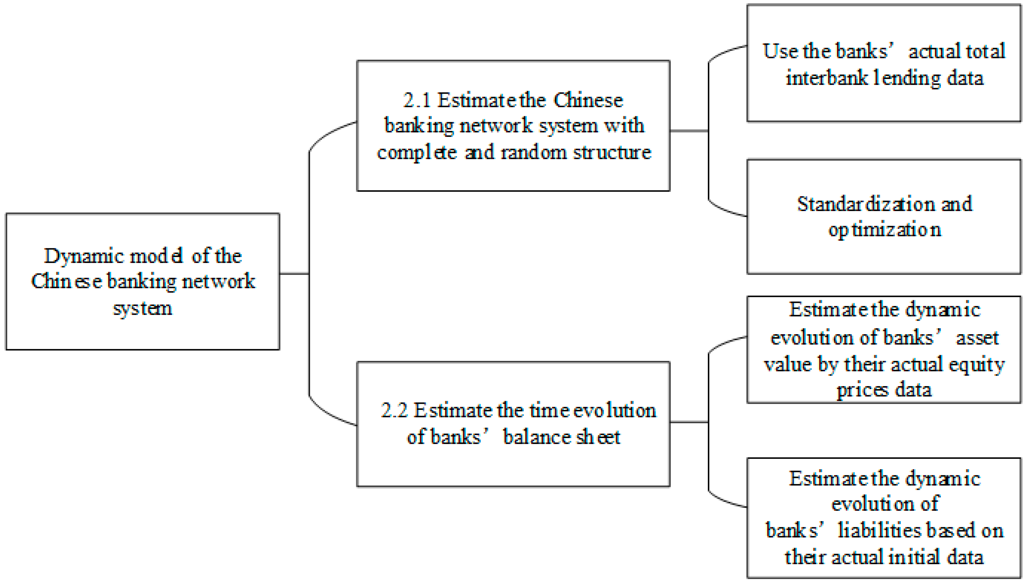
The framework of a dynamic Chinese banking network system is shown in Figure 1. It mainly contains two processes: the estimation of the interbank bilateral exposures matrix in the Chinese banking system with complete and random networks (the mathematical model is presented in Section 2.1) and the dynamic evolution of banks’ assets and liabilities (the mathematical model is presented in Section 2.2). In the first process, we need to generate a connectivity matrix ($16\times 16$) of complete and random networks, according to the network algorithm. The elements of connectivity matrix are 0 or 1, where 0 indicates that there is no connection between two banks, while 1 means there are interbank lending linkages between two banks. Then, we can estimate the bilateral exposures matrix of the Chinese banking network system with complete and random structures through the standardization and optimization based on the above connectivity matrix and the actual total interbank lending data of 16 listed banks from 2010 to 2015. In the second process, we use 16 Chinese listed banks’ historical stock price data to estimate the dynamic evolution of banks’ assets and use banks’ actual initial debt data to estimate the dynamic evolution of banks’ liabilities. With the evolution of the network structure and banks’ assets and liabilities at each time step, the dynamic evolution of the Chinese banking network system was formed.

2.1. Estimation of the Complete and Random Network

In the complete network, there is an edge between any two nodes, that is, any two banks have the interbank linkage in the banking system. In a random network, any two nodes attempt to connect with each other with a certain probability $p$ ($0<p<1$), that is, the probability that any two banks have the interbank linkage in the banking network system with a random structure, which is $p$ ($0<p<1$). Moreover, it’s the complete network if $p=1$.

In order to estimate the Chinese banking network system with complete and random structures, we need to obtain the interbank bilateral exposures matrix of the Chinese banking system. Due to the non-transparency of banks’ information, we cannot obtain the banks’ specific interbank exposures data. Only what we can get is the actual total interbank assets $a_i$ and the total interbank liabilities $b_i$ from the banks’ balance sheet. Therefore, the present paper uses the method commonly used in the study, i.e., Maximum Entropy (such as Elsinger et al. [25], Kanno [26], Gauthier et al. [12], and Fan et al. [27]) to minimize the uncertainty of banks’ interbank information in order to estimate the interbank bilateral exposures matrix of the banking network system. The interbank lending linkages could be represented by a ($N\times N$) nominal interbank matrix $X$, as shown in Equation (1).

$$X\begin{array}{ccccccccc}& & & & & & & & {\displaystyle \sum _j}\\ =& [& \begin{array}{c}{x}_{11}\\ ⋮\\ x_{i1}\\ ⋮\\ x_{N1}\end{array}& \begin{array}{c}\cdots \\ \ddots \\ \cdots \\ \ddots \\ \cdots \end{array}& \begin{array}{c}{x}_{1j}\\ ⋮\\ x_{ij}\\ ⋮\\ x_{Nj}\end{array}& \begin{array}{c}\cdots \\ \ddots \\ \cdots \\ \ddots \\ \cdots \end{array}& \begin{array}{c}{x}_{1N}\\ ⋮\\ x_{iN}\\ ⋮\\ x_{NN}\end{array}& ]& \begin{array}{c}{b}_1\\ ⋮\\ b_i\\ ⋮\\ b_N\end{array}\\ {\displaystyle \sum _i}& & a_1& \cdots & a_j& \cdots & a_N& & \end{array}$$

(1)

The element $x_{ij}$ in the matrix represents the lending loans of bank $j$ to bank $i$, the sum of elements in each row $b_i$ represents the total interbank liability of bank $i$, and the sum of elements in each column $a_j$ represents the total interbank assets of bank $j$, which is specifically described in Equation (2).

$$b_i={\displaystyle \sum _j{x}_{ij},a_j=}{\displaystyle \sum _i{x}_{ij}}.$$

(2)

We minimize the uncertainty of bank’s interbank bilateral exposure information by standardizing ${\displaystyle {\sum }_j{a}_j}={\displaystyle {\sum }_i{b}_i}=1$. Thus, we get $x_{ij}=a_j\ast b_i$, which represents the standardized lending loans of bank $j$ to bank $i$. We know that the diagonal elements of $X$ have to be zero, so we make new definitions for the elements $x_{ij}$ in the interbank matrix $X$ as the following.

$$x_{ij}^0=\{\begin{array}{ll}0,& \mathrm{i}=j,\\ a_j{b}_i,& \mathrm{otherwise}.\end{array}$$

(3)

When estimating the interbank bilateral exposures matrix of the banking system with complete and random structures, we introduce the connection matrix of complete and random networks that is generated at the beginning. Then the element “1” in the connection matrix is set by the non-zero value in Equation (3) while the element “0” in the connection matrix is set by zero in Equation (3). However, $X^0=(x_{ij}^0)$ in Equation (3) violates the summing constraints expressed in Equation (2). Therefore, we use the optimization algorithm (shown as Appendix A, and the details refer to Elsinger et al. [4]) to optimize the elements in the bilateral exposures matrix $X^0$, according to Equation (4). Then we can get the final bilateral exposures matrix of the Chinese banking system with complete and random structures.

$$\{\begin{array}{l}\min {\displaystyle \sum _{i=1}^N{\displaystyle \sum _{j=1}^N{x}_{ij}\ln }}\left(\frac{x_{ij}}{x_{ij}^0}\right)\\ {\displaystyle \sum _{j=1}^N{x}_{ij}=b_i,{\displaystyle \sum _{i=1}^N{x}_{ij}=a_j,x_{ij}\ge 0.}}\end{array}$$

(4)

2.2. Estimation of the Time Evolution of Banks’ Balance Sheet

Since the banks’ asset value cannot be observed every day, we could only obtain the data at the end of the year from banks’ balance sheets. However, the daily data of banks’ equity prices can be obtained from the stock market. In this case, we use a method to estimate the banks’ assets value of every day (i.e., the time evolution of assets value) by its daily equity data. In addition, the method has been used by Kanno [26], Liao et al. [13], and Fan et al. [27] to study the systemic risk of the banking system in Japan, Netherlands, and Kenya, respectively. By using the banks’ equity price data, the Black-Scholes model (Equation (7)), and maximization likelihood function (Equation (10)), we could estimate the drift rate and volatility rate of banks’ assets value, and then obtain the time evolution of banks’ assets value, according to the stochastic model (Equation (6)).

Assuming that the asset value $V_i$ of bank $i$ follows a geometric Brownian motion (this model has been widely used to simulate the movement of the stock market) with a drift rate ${\mu }_i$ and a volatility rate ${\sigma }_i$ described as follows.

$$d{V}_i=u_i{V}_{i}dt+{\sigma }_i{V}_i{d}_{{\rm Z}}.$$

(5)

Based on the time series data from the stock market, the Geometric Brownian Motion aims to estimate the drift rate and variance of banks’ asset value. In addition, the actual time series data used to estimate it is about one year. Therefore, the estimated asset value will not deviate too much if the stock market is in a crisis moment, which will have an impact on the estimated results. Yet, the impact will not be too great. The solution to Equation (5) is obtained as the formula below.

$$V_i(t)=V_i(0){\mathrm{e}}^{u_i-({\sigma }_i^2/2)th+{\sigma }_i\sqrt{th\ast {{\rm Z}}_i}(t)},$$

(6)

where $z_i(t)$ obeys normal distribution ($N(0,1)$) and if we know ${\mu }_i$ and ${\sigma }_i$, then we will get the time evolution of $V_i$ according to Equation (6).

As mentioned in Lehar [3], a bank’s equity can be interpreted as a call option on a bank’s assets. Therefore, we can use a time series of observed equity prices of banks and balance sheet information to obtain the dynamic evolution of banks’ asset value. Here, we use the Black-Scholes model [28] to estimate ${\mu }_i$ and ${\sigma }_i$ as follows.

$$S_t(t)=V_i(t)\varphi (d_t)-L{D}_i(t)\varphi (d_t-{\sigma }_i\sqrt{T}),$$

(7)

$S_t(t)$ is the equity value of bank $i$, which can be obtained from the stock market. $\varphi (•)$ is the standard normal distribution function. $T$ is the business day of the stock market, which is equal to 220 days. $L{D}_i(t)$ is bank i’s debt with a maturity of $t$, which is assumed to be insured and, therefore, grow at the risk-free interest rate $r$.

$$L{D}_i(t)=L{D}_i(0)e^{rt},$$

(8)

$t$ represents the evolution of days and

$$d_t=\frac{\ln (V_i(t)/D_i(t))+(\frac{1}{2}{\sigma }_i^2)T}{{\sigma }_i\sqrt{T}}.$$

(9)

Given $V_i(0)$ and the time series data of bank equity prices $\left\{S_i(0),S_i(1),\dots ,S_i(T)\right\}$ observed from the stock market, the time series data of bank debt $\left\{L{D}_i(0),L{D}_i(1),\dots ,L{D}_i(T)\right\}$ calculated by Equation (8) (the face value of bank debt $L{D}_i(0)$ is observed from the balance sheet), we can estimate the time series value of the bank assets $\left\{{\widehat{V}}_i(1),{\widehat{V}}_i(2),\dots ,{\widehat{V}}_i(T)\right\}$, according to Equation (7). By setting the arbitrary initial value of ${\mu }_i(0)$ and ${\sigma }_i(0)$, we can use the following maximization likelihood function proposed by Duan et al. [29] to estimate ${\mu }_i$ and ${\sigma }_i$ of bank i.

$$L(u_i,{\sigma }_i;{\widehat{V}}_i(1),{\widehat{V}}_i(2),\dots ,{\widehat{V}}_i(T))=-\frac{T}{2}\ln (2\pi {\sigma }_i^{2}h)-\frac{T}{2}{\displaystyle \sum _{k=1}^T\frac{{(R_i(k)-(u_i-\frac{{\sigma }_i^2}{2})h)}^2}{{\sigma }_i^{2}h}-{\displaystyle \sum _{k=1}^T\ln {\widehat{V}}_t}},$$

(10)

where $R_i(k)=\ln ({\widehat{V}}_i(t)/{\widehat{V}}_i(t-1)),h=1/220$. Lastly, we can get the time evolution of $V_i$ by taking ${\mu }_i$ and ${\sigma }_i$ into Equation (6).

The total liabilities of bank $i$ in the banking network system can be described by the equation below.

$$D_i(t)=(V_i^{}(0)-C_i(0))e^{rt},$$

(11)

where $r$ is the risk-free interest rate for each day and $C_i(0)=7\%\ast V_i(0)$, $C_i(0)$ is the initial capital of bank $i$.

2.3. The Default of Banks

In the present paper, we consider bank $i$ default when it is insolvent, which satisfied Equation (12) as follows:

$$V_i(t)+a_i(t)-D_i(t)-b_i(t)<0,$$

(12)

where bank i’s total interbank assets $a_i(t)$ and total interbank liabilities $b_i(t)$ are affected by contagious risk in the interbank market, and the difference between the interbank assets $a_i(t)$ and interbank liabilities $b_i(t)$ is the liquidity of bank $i$ in the model of this paper. Therefore, there are two kinds of banks’ default in the present paper. One is the basic default from bank $i$ own insolvency ($V_i(t)-D_i(t)$). The other is contagious default caused by the lack of liquidity affected by interbank lending. This paper measures the sum of the two kinds of defaults, namely, banks’ total default. In this scenario, we extend the clearing payment mechanism proposed by Eisenberg and Noe [4] to determine the payment of banks’ debt in the dynamically evolving banking network system. We define a new matrix $\prod \in {[0,1]}^{N\times N}$ to standardize the total interbank liabilities as follows.

$${\prod }_{ij}(t)=\{\begin{array}{ll}{x}_{ij}(t)/b_i(t)& b_i(t)>0,\\ 0& otherwise,\end{array}$$

(13)

where $b_i(t)={\displaystyle \sum _j{x}_{ij}}(t)$ means the total interbank liabilities of bank $i$ at time step t. We define a clearing payment vector $p_i^{\ast }(t)$ that respects bank i’s limited liability and proportional sharing in case of default. It denotes bank i’s total payments under the clearing mechanism, which is defined as follows.

$$p_i^{\ast }(t)=\{\begin{array}{l}{b}_i(t){\displaystyle \sum _{j=1}^N{\mathsf{\Pi }}_{ij}^{\prime }(t)p_j^{\ast }(t)+e_i(t)\ge b_i(t)},\\ {\displaystyle \sum _{j=1}^N{\mathsf{\Pi }}_{ij}^{\prime }(t)p_j^{\ast }(t)+e_i(t)0\le {\displaystyle \sum _{j=1}^N{\mathsf{\Pi }}_{ij}^{\prime }(t)p_j^{\ast }(t)+e_i(t)<b_i(t)},}\\ 0{\displaystyle \sum _{j=1}^N{\mathsf{\Pi }}_{ij}^{\prime }(t)p_j^{\ast }(t)+e_i(t)<0},\end{array}$$

(14)

and,

$$e_i(t)=V_i(t)-D_i(t).$$

(15)

In this case, we adopt the default algorithm in Eisenberg and Noe [4] to find a clearing payment vector $p_i^{\ast }$. In addition, we should note that when bank $i$ defaults, bank $i$ can pay only a part of its interbank liabilities to other banks. The ratio is defined as follows.

$${\chi }_i=\frac{{\displaystyle \sum _{j=1}^N{\mathsf{\Pi }}_{ij}^{\prime }(t)p_j^{\ast }(t)+e_i(t)}}{b_i(t)}.$$

(16)

Thus, the default of bank i has an impact on the total assets and total liabilities of its debt bank j because of the interbank lending, and they are updated in accordance with Equation (17) as follows.

$$\begin{array}{l}{V}_j(t+1:T)=V_j(t)-{\chi }_i\ast x_{\begin{array}{l}ij\\ \end{array}},\\ D_j(t+1:T)=D_j(t)-{\chi }_i\ast x_{\begin{array}{l}ij\\ \end{array}}.\end{array}$$

(17)

Meanwhile, setting up its interbank linkages $x_{i,j}(t)=0$ after bank $i$ default, and then re-estimate the bilateral exposures matrix. Moreover, the total interbank assets and total interbank liabilities of the debt bank $j$ are updated, according to Equation (18).

$$\begin{array}{l}{a}_j(t+1)={\displaystyle \sum _{i=1}^N{x}_{i,j}(t+1),}\\ b_j(t+1)={\displaystyle \sum _{j=1}^N{x}_{i,j}(t+1)}.\end{array}$$

(18)

According to Equations (17) and (18), we note that, in the banking network system model of this paper, a bank’s assets and liabilities are dynamically changing at each time step and are also affected by the interbank linkages. Once a bank defaults, its debt banks’ total assets, total liabilities, interbank lending assets, and interbank liabilities will be updated and the other banks’ interbank lending linkages with the default bank are updated to 0, accordingly. The default bank is cleared out of the banking system. The rest banks re-generate new interbank lending linkages at the next time step, so the bank’s network is updated dynamically in this way.

After the banks’ total assets, total liabilities, total interbank assets, and the total interbank liabilities are updated, we judge again that whether the bank is default, according to Equation (12). The evolution of the banking network system is stopped when all banks default in each simulation scenario.

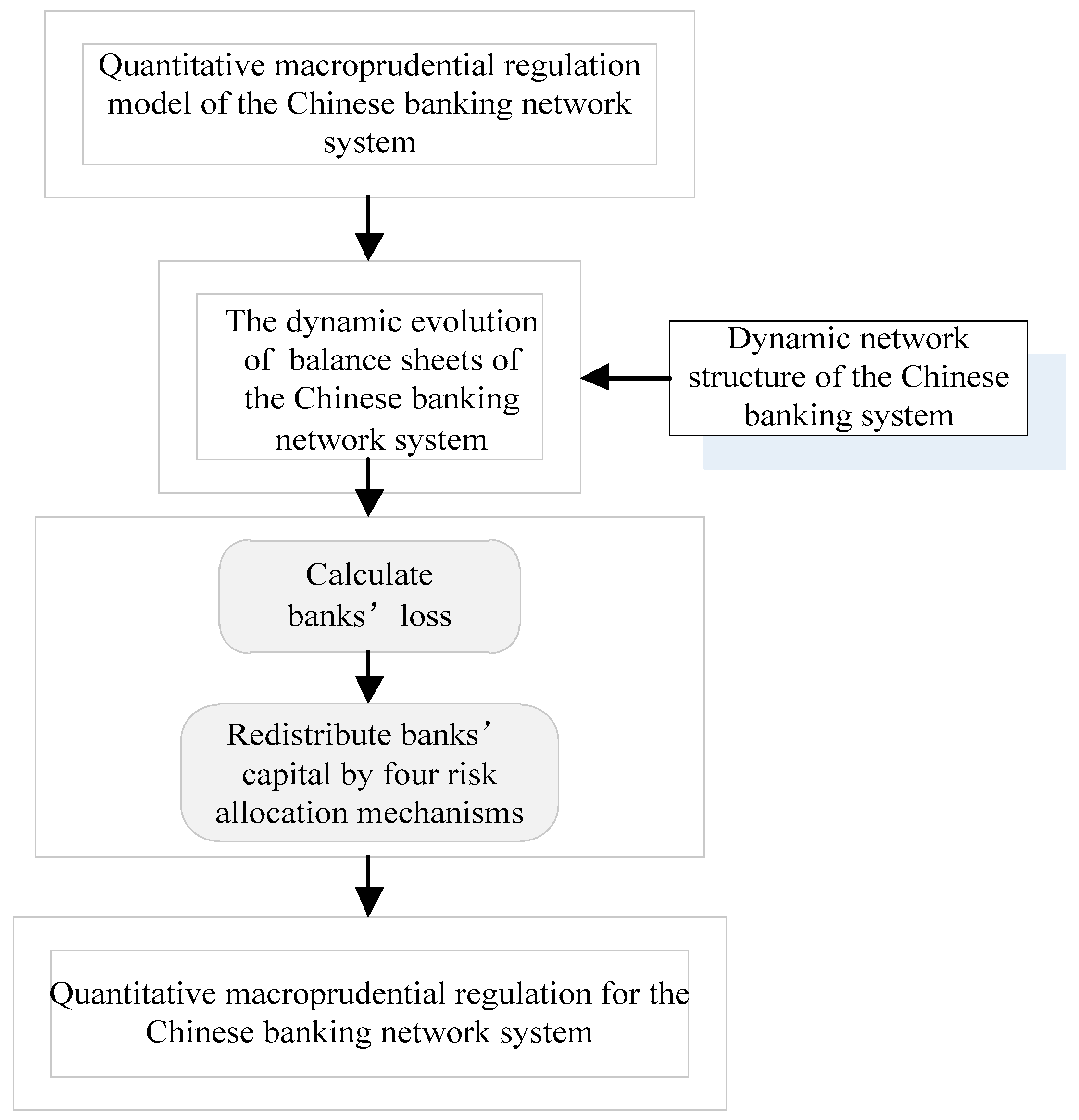
3. The Model of Macroprudential Regulation

Figure 2 is the quantitative model of macroprudential regulation for the Chinese banking network system. The model is constructed based on the dynamic evolution of the Chinese banking network system, that is, we calculate the banks’ losses based on the dynamic evolution of the network structure and the balance sheet at first, and then introduce four risk allocation mechanisms to calculate the banks’ macro-prudential capital. Thus, we can implement macro-prudential capital requirements for the Chinese banking network system (the mathematical model is presented in Section 3).

The core of calculating banks’ macro-prudential capital $C$ lies in measuring banks’ losses $l$. The banks’ total assets, total liabilities, the total interbank assets, and the total interbank liabilities evolve with time step t in each simulation, where banks’ losses at each time step are set by Equation (19), and $e_i(t)$ in Equation (19) is calculated according to Equation (15) in Section 2.3.

$$l_i(t)=\min ({\displaystyle \sum _{j=1}^N{\mathsf{\Pi }}_{ij}^{\prime }(t)p_j^{\ast }(t)+e_i(t)-b_i(t)},0).$$

(19)

The dynamic evolution ($t$ time steps) of the banking network system is iterated for $test$ of times ($test=1,2,3\dots m$) and $l_{i,test}(t)$ represents the loss of bank $i$ at each time step of one time simulation. Therefore, we can get a N × m loss matrix that $N$ banks in m times of simulation. The loss matrix under the given capital C_i = (C₁,C₂,…C_N) can be expressed as $l(C)$. Then, we use the risk allocation mechanism $f(•)$ to allocate systemic risk to every bank, which is described as f_i(l(C)). Therefore, the macroprudential capital of bank $i$ is calculated as follows.

$$\{\begin{array}{l}{C}_i^{*}=f_i(l(C_i^{*}))\times ({\displaystyle \sum _{i=1}^N{C}_i^0})\\ {\displaystyle \sum _{i=1}^N{f}_i(l(C))=1,f_i(l(C))\ge 0,}\end{array}$$

(20)

where $C_i^0$ is the initial capital of bank $i$ and $C_i^{\ast }$ is the redistributed capital of bank $i$. The banks’ default probability are set as the ratio of the number of bank default and the total number of simulations $m$.

3.1. Four Risk Allocation Mechanisms

Following Gauthier et al. [12] and Liao [13], we use the following four risk allocation mechanisms (Component VaR, Incremental VaR, Shapley value EL, and ΔCoVaR) to calculate each bank’s macroprudential capital.

3.1.1. Component VaR

The core of the mechanism is to reallocate banks’ capital based on the contribution $\beta$ of each bank’s loss $l_i$ to the total loss of the banking network system ${\displaystyle {\sum }_{i=1}^n{l}_i}(l_p)$ and ${\beta }_i=\frac{\mathrm{cov}(l_i,l_p)}{{\sigma }^2(l_p)}$.

The macroprudential capital of bank $i$ under the Component VaR mechanism is given by the equation below.

$$C_i^{CVaR}={\beta }_i{\displaystyle \sum _{i=1}^n{C}_i^0}.$$

(21)

The changes in the capital of bank $i$ under the Component VaR mechanism is calculated by $(C_i^{CVaR}-C_i^0)/C_i^0$.

3.1.2. Increment VaR

The core of the mechanism is to reallocate banks’ capital, according to the change in the overall risk due to the exclusion of a bank in the system.

The banking network system simulated over 10,000 scenarios and, for each scenario, we compute the 5% VaR of the total losses $l_p$ in the system, denoted by $Va{R}_p$. Then, we calculate the 5% VaR of the total losses excluding bank $i$ denoted by $Va{R}^{-i}$. Therefore, the increment VaR of bank $i$ is calculated by the equation below.

$$IVa{R}_i=Va{R}_p-Va{R}^{-i}.$$

(22)

The macroprudential capital of bank $i$ under the increment VaR mechanism is given by the equation below.

$$C_i^{IVaR}=\frac{IVa{R}_i}{{\displaystyle \sum _{i=1}^{n}IVa{R}_i}}{\displaystyle \sum _{i=1}^n{C}_i^0}.$$

(23)

The changes in the capital of bank $i$ under the increment VaR mechanism is $(C_i^{IVaR}-C_i^0)/C_i^0$.

3.1.3. Shapley Value EL

The Shapley value EL mechanism is the arithmetic average of $n$ times of simulation based on the increment VaR mechanism. So, new $IVa{R}_i$ is represented as ${\varphi }_i$ by the calculation of arithmetic average based on $Va{R}_p$ and $Va{R}^{-i}$.

The macroprudential capital of bank $i$ under the Shapley value EL mechanism is given by the equation below.

$$C_i^{ShapleyEL}=\frac{{\varphi }_i}{{\displaystyle \sum _{i=1}^n{\varphi }_i}}{\displaystyle \sum _{i=1}^n{C}_i^0}.$$

(24)

The changes in the capital of bank $i$ under the Shapley value EL mechanism is $(C_i^{ShapleyEL}-C_i^0)/C_i^0$.

3.1.4. ΔCoVaR

Following Adrian and Brunnermeier [30], CoVaR of bank $i$ is defined as the total loss of the banking network system conditional on bank $i$, which realizes a loss corresponding to its VaR. CoVaR_i can be described by the equation below.

$${\mathrm{Pr}(\mathrm{l}}_{\mathrm{p}}<{\mathrm{CoVaR}}_{\mathrm{i}}|{\mathrm{l}}_{\mathrm{i}}\in [(1-\mathsf{𝓁}){\mathrm{VaR}}_{\mathrm{i}},(1+\mathsf{𝓁}){\mathrm{VaR}}_{\mathrm{i}}])=0.5\%,\mathsf{𝓁}=0.1,$$

(25)

where $\Delta {\mathrm{CoVaR}}_{\mathrm{i}}$ is defined as the difference of ${\mathrm{CoVaR}}_{\mathrm{i}}$ and the VaR of the total losses in the banking network system conditional on bank $i$, which makes a loss at its median. Therefore, it is expressed by the formula below.

$$\Delta {\mathrm{CoVaR}}_{\mathrm{i}}={\mathrm{CoVaR}}_{\mathrm{i}}-({\mathrm{VaR}}_{\mathrm{p}}|{\mathrm{l}}_{\mathrm{i}}=\mathrm{median}({\mathrm{l}}_{\mathrm{i}})).$$

(26)

The macroprudential capital of bank $i$ under the ΔCoVaR mechanism is given by the equation below.

$$C_i^{\Delta CoVaR}=\frac{\Delta CoVa{R}_i}{{\displaystyle \sum _{i=1}^n\Delta CoVa{R}_i}}{\displaystyle \sum _{i=1}^n{C}_i^0}.$$

(27)

The changes in the capital of bank i under the ΔCoVaR mechanism is $(C_i^{\Delta CoVaR}-C_i^0)/C_i^0$.

4. Data

In the present paper, we collect 16 listed banks’ balance sheet data and the stock prices data in China from 2010 to 2015. It should be noted that the Agricultural Bank of China (Beijing, China) and China Everbright Bank (Beijing, China) were both listed in 2010. Thus, the bank number ($BN$) in 2010 is set as $BN=14$ and $BN=16$ from 2011 to 2015 in our simulated banking network system. In addition, the size of 16 listed banks is different, and they present different characteristics. Moreover, we mainly calculate bank’s macroprudential capital according to the contribution of each bank to the systemic risk of the whole banking system. The existing related studies such as Gauthier et al. [12] and Liao et al. [13] also used several risk allocation mechanisms to calculate the bank’s macroprudential capital requirements. Their samples are six banks in Canada and four banks in the Netherlands, respectively. However, their research did not consider the interbank network structure that we have considered in the present paper. The 16 listed banks we choose in this paper are large listed banks. The sum of their total assets accounts for more than 60% of the total assets of the Chinese banking industry. (Chinese banking industry includes state-owned commercial banks, joint-stock commercial banks, city commercial banks, and postal savings banks, etc., among which state-owned commercial banks and joint-stock commercial banks are major commercial banks. The 16 listed banks used in this paper include all the five state-owned commercial banks, eight joint-stock commercial banks, and three city commercial banks. The assets of these banks are large among all listed banks.). We aim at using these banks’ actual data to verify that the macroprudential regulation method used in this paper is effective and feasible. The number of banks in this study affects the results of the paper, but do not affect the verification of the macro-prudential regulation method. The banks’ initial capital $C0$ is set to 7% of its initial total assets referred to the Basel agreement. Set the total simulation times m = 10,000 in the banking network system. 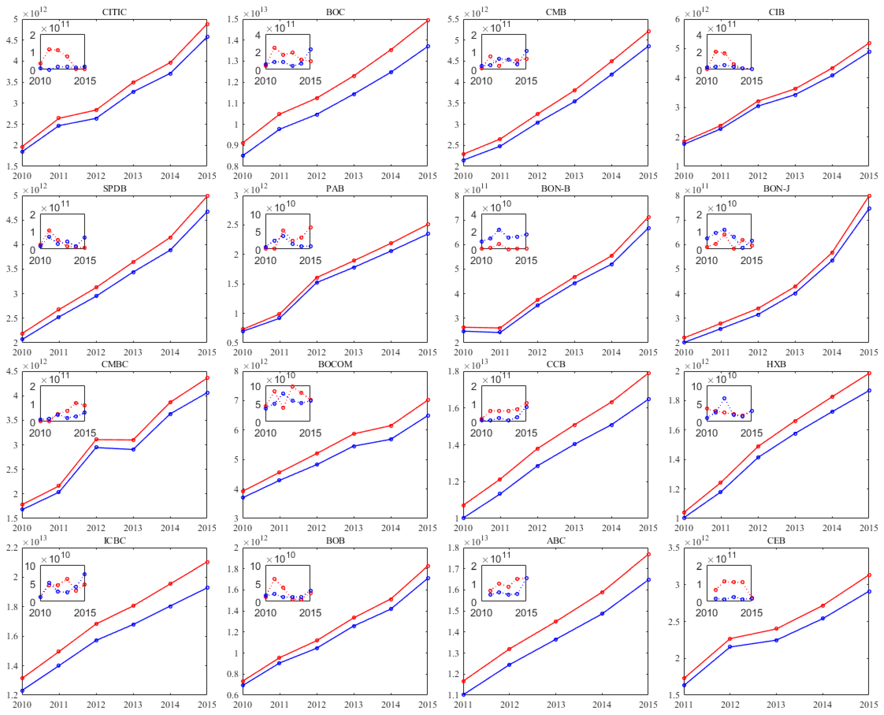We mainly use the data of banks’ total assets ($V$), total liabilities (LD), the interbank assets (a), and interbank liabilities (b) for initialization in the banking network model and estimation of the bilateral exposures matrix. The data is shown in Figure 3. It can be found that every bank’s total assets and liabilities are generally increasing from 2010 to 2015, and the total assets are slightly higher than the total liabilities. Moreover, the size of the Bank of China (BOC) (Beijing, China), the China Construction Bank (CCB) (Beijing, China), the Industrial and Commercial Bank of China (ICBC) (Beijing, China), the Agricultural Bank of China (ABC), and the Bank of Communications (BOCOM) (Shanghai, China) are relatively large among all banks. These banks’ total assets are more than or close to 10¹³. While, the size of the Bank of Ningbo (BON-B) (Ningbo, China) and the Bank of Nanjing (BON-J) (Nanjing, China) are relatively small. Their total assets are both less than 10¹². The following are PingAn Bank (PAB) (Shenzhen, China), Huaxia Bank (HXB) (Beijing, China), and China Everbright Bank (CEB). Their total assets are all lower than 5*10¹². In addition, the inline subgraph in Figure 3 shows that the interbank lending of banks varies year to year and it is clear that the interbank lending assets of the Bank of China (BOC) and the Industrial Bank Co., Ltd (CIB) (Fuzhou, China) are the largest from 2011 to 2012, and that of Bank of Ningbo (BON-B) and Bank of Nanjing (BON-J) are the smallest every year. We find that the interbank lending assets of the Bank of Ningbo (BON-B) and the Bank of Nanjing (BON-J) are lower than their interbank lending liabilities from 2010 to 2015.

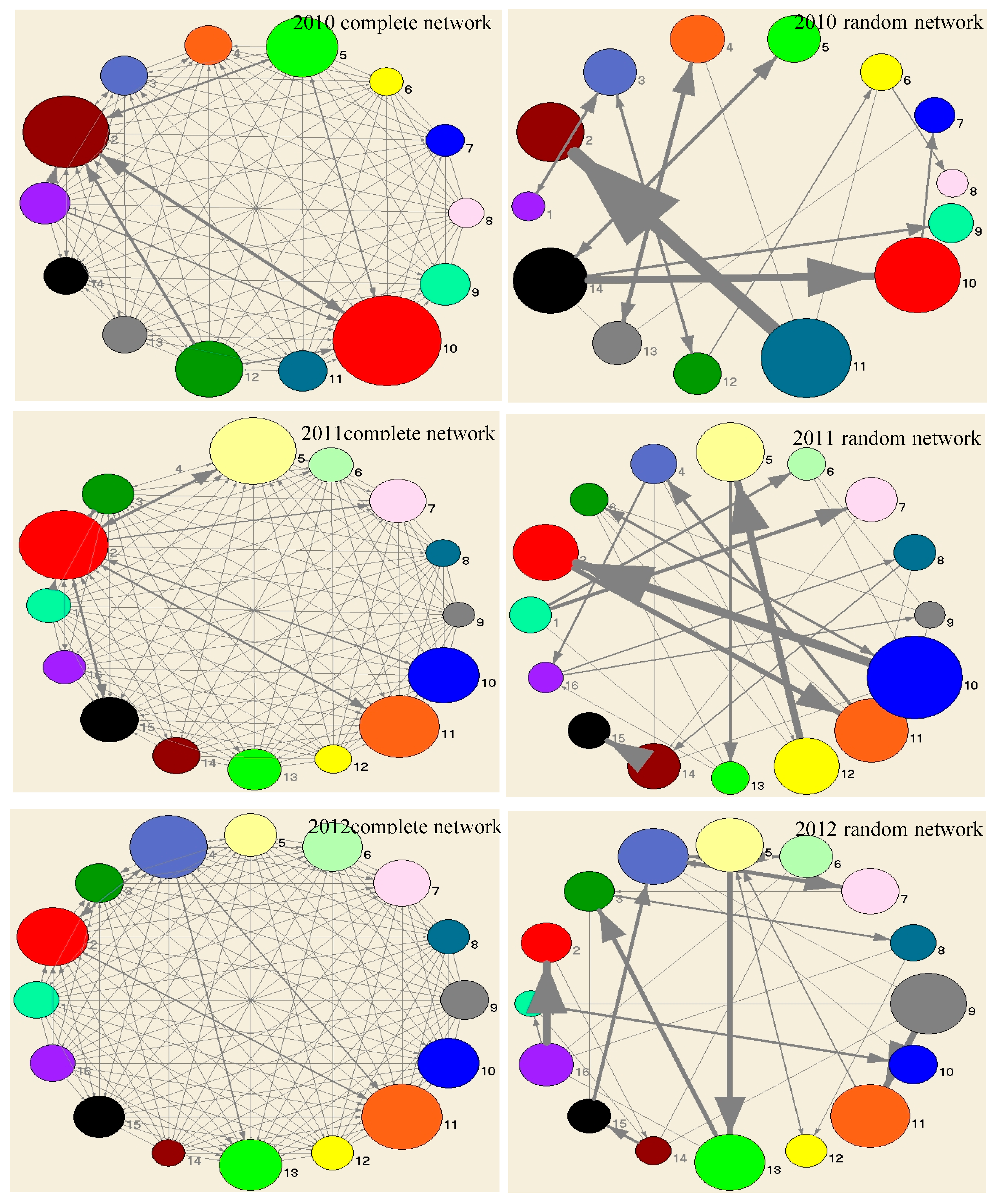
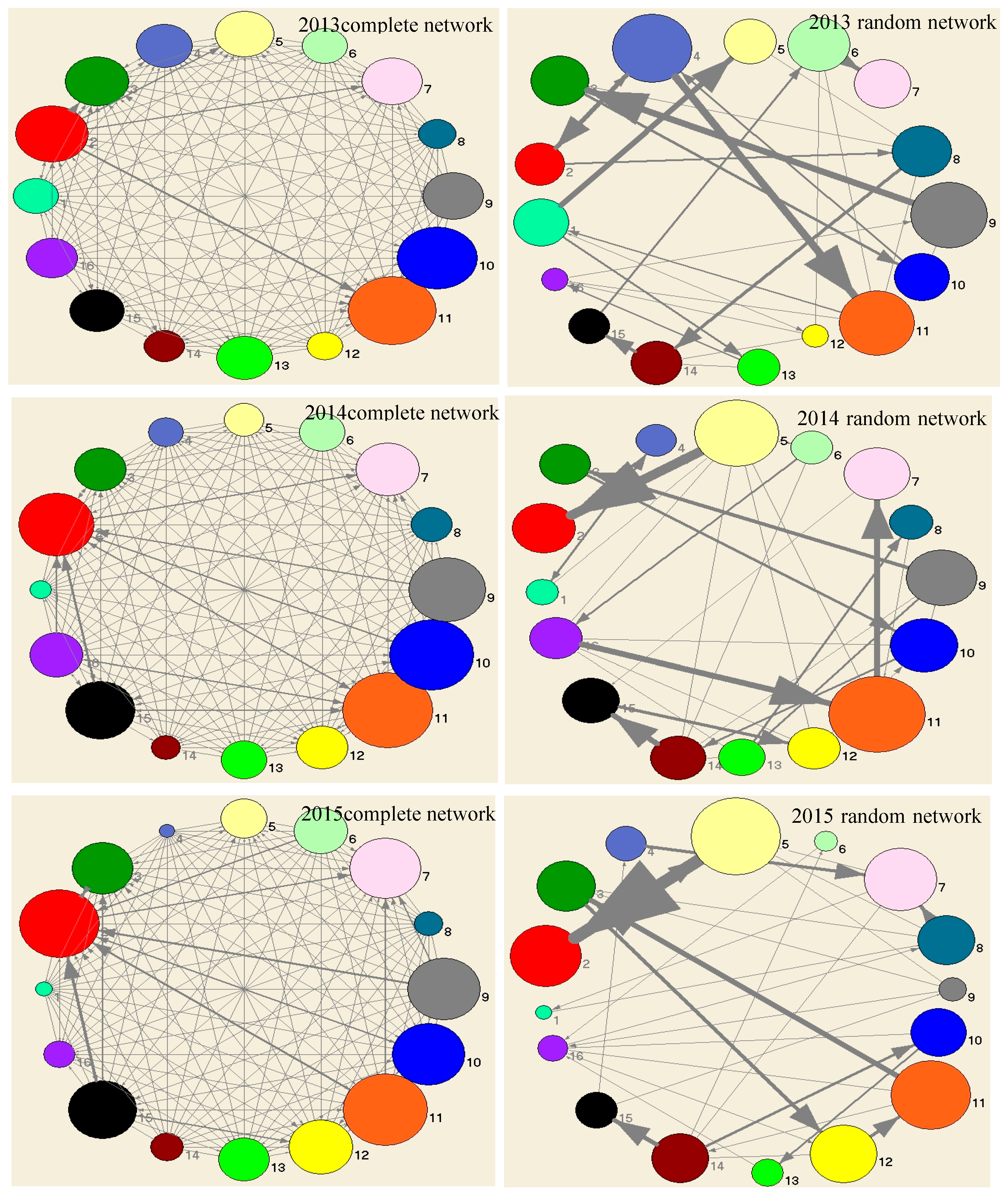
After the dynamic evolution of the banking network system under the initial capital based on banks’ initial actual data of the total interbank assets and interbank liabilities, we get its specific complete and random network structures from 2010 to 2015, which is shown in Figure 4. As can be seen from Figure 4, first, the interbank lending of Bank of China, China Construction Bank, and Agricultural Bank of China are all relatively large in the banking system with complete and random networks in most years from 2010 to 2015. In addition, there are also Bank of Communications, Bank Of Ningbo, China Minsheng Banking (Beijing, China), and Shanghai Pudong Development Bank (Shanghai, China) (2010–2011) in complete network, and also Shanghai Pudong Development Bank and Industrial Bank Co., Ltd in random network. Moreover, the China Construction Bank has many interbank linkages in a random network while the interbank linkage of the Bank of China is lower and the Agricultural Bank of China is not clear. Second, the interbank lending of the Bank Of Nanjing and China CITIC Bank (Beijing, China) are relatively small in the banking system with the two networks in most years. Additionally, there are PingAn Bank and Bank Of Ningbo (2010–2011) as well as Industrial Bank Co., Ltd (2014–2015) in a complete network. There is also the PingAn Bank in a random network. Moreover, the interbank linkages of China CITIC Bank and Bank Of Ningbo are less in a random network in most years and the PingAn Bank is not clear. Lastly, the Bank of Beijing (Beijing, China) is more prominent in the two networks since its interbank lending is relatively small in the banking system with a complete network in most years, while it is relatively large in a random network and has many interbank linkages.

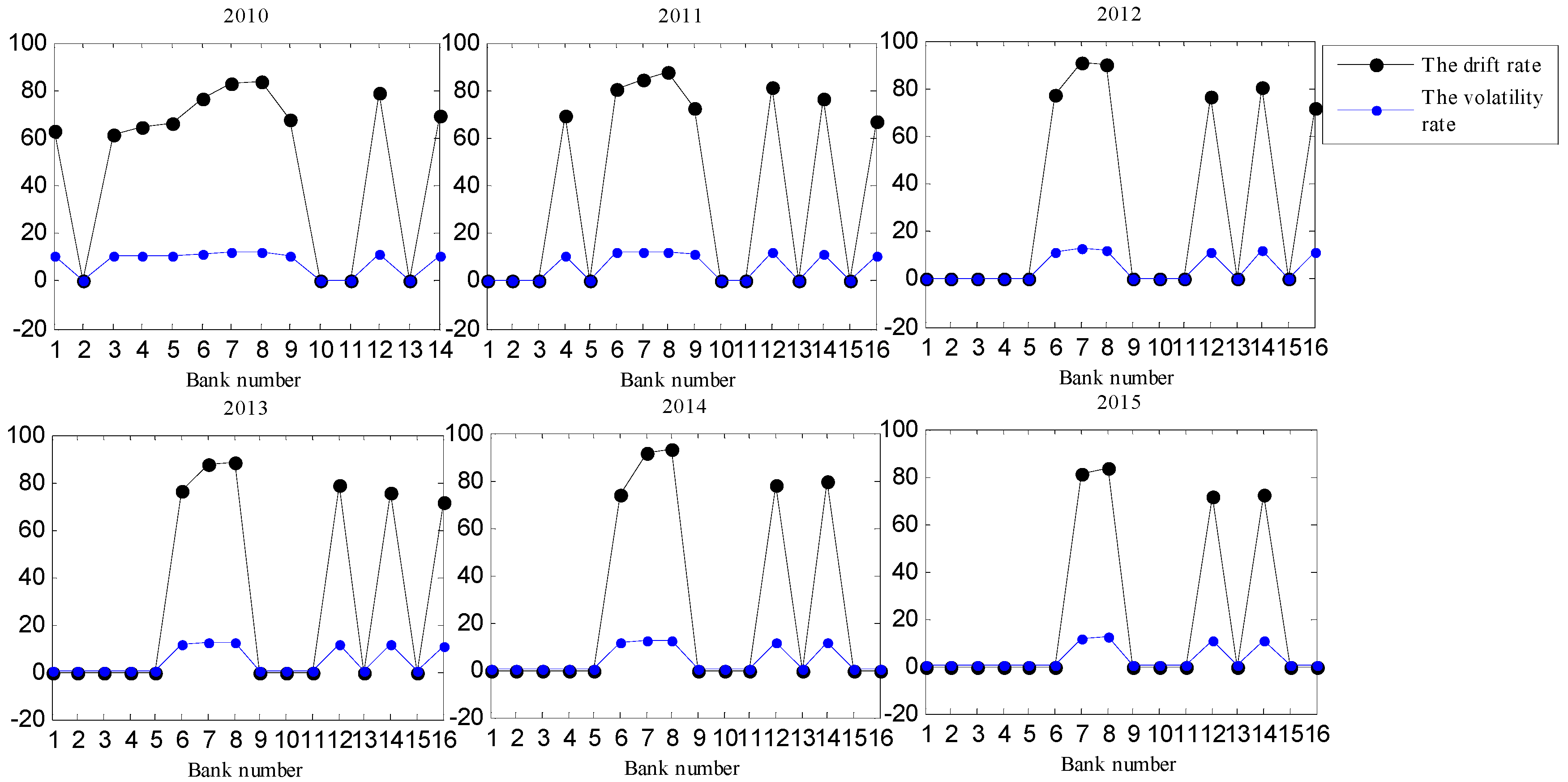
Meanwhile, according to the parameter estimation process by using banks’ stock data and the maximization likelihood function in chapter 3, we obtain the drift rate ${\mu }_i$ and volatility rate ${\sigma }_i$ of banks’ asset value every year, as shown in Figure 5. It is clear that the drift rate ${\mu }_i$ and volatility rate ${\sigma }_i$ of PingAn Bank, Bank of Ningbo, Bank of Nanjing, Huaxia Bank, and Bank of Beijing are relatively high among the 16 banks from 2010 to 2015. Therefore, the asset value of these banks fluctuates largely every year while the rest of the banks are stable.

5. Results

5.1. Changes in Capital

According to the formula in Section 3.1 $(C_i^{\ast }-C_i^0)/C_i^0$, we obtain the changes in banks’ capital under the four risk allocation mechanisms and the initial capital (see Figure 6).

First of all, it can be seen from Figure 6 that the majority of banks’ capital has increased and a small number of banks’ capital decreased in the banking system with complete and random structures under the four risk allocation mechanisms from 2010 to 2015. The number of banks whose capital decreased under the Incremental VaR and Shapley value EL mechanisms is more than that of the Component VaR and ΔCoVaR mechanisms, but the changes in banks’ capital (increase or decrease) are much lower than that of the Component VaR and ΔCoVaR mechanisms. Moreover, the changes in part of banks’ capital are clearly different in the two networks under the Component VaR and Incremental VaR mechanisms from 2010 to 2013, while they are close in the other cases. Generally the influence of the two network structures on the change in banks’ capital under the Component VaR mechanism is relatively greater.

Then, we analyzed the changes in banks’ capital in detail. (1) The bank’s capital decreased. According to Figure 6, there are the Bank of China, the Bank of Communications, the China Construction Bank, the Industrial and Commercial Bank of China, and the Agricultural Bank of China whose capital decreased in the banking system with complete and random networks under the four mechanisms from 2010 to 2015, especially the China Construction Bank and the Industrial and Commercial Bank of China, which have reduced the most under the Component VaR and ΔCoVaR mechanisms, which reduced by about 60% to 75% and it is about 5% to 30% under the other two mechanisms. In addition, the capital of PingAn Bank Bank Of Ningbo, and Bank Of Nanjing decreased under the Incremental VaR mechanism in a complete network in 2010 and 2012, and the capital of China CITIC Bank, the China Merchants Bank Ltd (Shenzhen, China), the Industrial Bank Co., Ltd, the Shanghai Pudong Development Bank, China Minsheng Banking, and the China Everbright Bank decreased in the two networks under the Shapley value EL mechanism from 2014 to 2015. (2) While the other banks’ capital are all basically increased in the other cases, it is found that some banks’ capital has a significant increase under the Component VaR and ΔCoVaR mechanisms, especially the Bank Of Ningbo and the Bank Of Nanjing, which have increased both by more than or close to 100% from 2010 to 2015. The capital of the PingAn Bank, the Huaxia Bank, and the Bank of Beijing, China Everbright Bank has increased by about 100%-500%, while it is within 100% under the Incremental VaR and Shapley value EL mechanisms. Furthermore, it is found that the capital of PingAn Bank, Bank Of Ningbo, and Bank Of Nanjing changes by comparing it with a complete network and a random network under the Component VaR and Incremental VaR mechanisms in 2010, 2012, and 2013, while it is not clear with the two networks in other cases.

5.2. The Default Probability of Banks under the Initial Capital and Four Risk Allocation Mechanisms

First, we discuss each bank’s default probability in the banking system with complete and random networks under the initial capital from 2010 to 2015 (see Figure 7). It is found that the default banks are the most from 2010 to 2011 in the two networks and each bank’s default probability is the highest in 2010, especially the default probability of the Bank Of Ningbo in a random network, which is close to 2.5%. In this case, we know that its interbank lending is not clear and it has little interbank linkages, according to Figure 4. There are mainly the PingAn Bank, the Bank Of Ningbo, the Bank Of Nanjing, the Huaxia Bank, the Bank of Beijing, and the China Everbright Bank that often default among the 16 banks during the six-year period. Moreover, some banks’ default probability is significantly different between the two networks, such as the Bank Of Ningbo in 2010 and 2014, the Huaxia Bank in 2011, Bthe ank of Beijing in 2012, and the Bank Of Nanjing in 2015. These banks’ default probability in a complete network is significantly lower than that of the random network while the default probability of the PingAn Bank in 2011 and 2013, the Industrial Bank Co., Ltd in 2010, the Huaxia Bank in 2012 and 2013, and the Bank Of Ningbo in 2015 in a complete network is significantly higher than that of the random network. Furthermore, we study the stability of the entire banking system with complete and random networks by calculating the average default probability of all banks (see Figure 8). It is found that the banking system is the most unstable in 2010. Its average default probability is basically reduced year by year from 2010 to 2014. In addition, the average default probability of the banking system with a complete network is clearly higher than that of the random network in 2013, while it is the opposite in 2014, and it is not clear in the other years.

Then, it is found that most banks’ default probability is reduced every year under the four risk allocation mechanisms by comparing the colorful marks with a black mark in Figure 9. However, there are individual banks whose default probability under the redistributed capital is unexpectedly higher than that of the initial capital in some cases, which are the Shanghai Pudong Development Bank under the Component VaR mechanism, the Bank Of Nanjing under the Shapley value EL mechanism in a random network in 2010, the PingAn Bank in 2010, the Bank Of Ningbo in 2010 and 2012, and the Bank Of Nanjing in 2010, 2012, and 2013 under the Incremental VaR mechanism in a complete network. We find that these banks have defaulted under the initial capital, especially the Bank Of Ningbo and the Bank Of Nanjing whose default probability is relatively high. However, their capital has reduced under the four risk allocation mechanisms. The Bank Of Ningbo has reduced the most in 2010 (by about 80%). To sum up, these banks have been already relatively fragile under the initial capital. In addition, their capital have been further reduced after the readjustment. At the same time, they have relatively weak interbank linkages in the interbank market. Therefore, their situation cannot be improved. However, the capital of the Bank of China, the China Construction Bank, the Industrial and Commercial Bank of China, and the Agricultural Bank of China have also been reduced under each mechanism every year in addition to individual cases, but their default probabilities have not increased. This is because these banks do not default under the initial capital, which indicates that these banks themselves are relatively robust and they have relatively large interbank linkages with many banks, which help them to resist risks.

5.3. Regulatory Analysis and Enlightenment

This paper mainly calculates banks’ macro-prudential capital quantitatively (the simulation results in Section 5.1) and then analyzes the banks’ macro-prudential regulation effect by comparing the banks’ default probability under the macro-prudential capital and that under the initial capital (the simulation results in Section 5.2). In Section 5.3, we try to explore the inherent laws of the banks’ macro-prudential regulation using the results in Section 5.1 and Section 5.2, and give some policy implications.

In order to measure the macro-prudential regulation effect on the whole banking system with complete and random networks under the four mechanisms, we calculate the average default probability for all banks and the results are shown in Figure 10. It can be seen from Figure 10 that the macro-prudential regulation on the banking system with a complete network under the Incremental VaR mechanism in 2010 is not effective (the average default probability of the banking system under the redistributed capital is higher than that of the initial capital), while the four mechanisms all effectively reduce the average default probability of the banking system in the other cases, which shows a good regulation effect. In addition, it is found that the average default probability of the banking system with a complete network is significantly higher under the Incremental VaR mechanism in 2010, 2012, and 2013 than that of the random network, while it is slightly higher in a random network under the Shapley value EL and Component VaR mechanisms in 2010. It is not clear in the other cases. Generally, the ΔCoVaR mechanism has the best regulation effect. The average default probability of the banking system each year under this mechanism in the two networks is basically 0, which shows that the banking system under this mechanism is not affected by the two network structures. This is followed by the Component VaR and the Shapley value EL mechanisms, respectively. Lastly, the average default probability of the banking system with a complete network in 2010 under the Incremental VaR mechanism is higher than that of the initial capital and they are close in 2012.

There is a relatively significant difference between the two networks in the default probability of the banking system under the Incremental VaR, Shapley value EL, and Component VaR mechanisms from 2010 to 2013, while it has little difference under the ΔCoVaR mechanism. This indicates that the macro-prudential regulation for the banking system under the ΔCoVaR mechanism is not affected by the two network structure, so this mechanism has strong applicability. The banking system is easily affected by the two network structures under the other mechanisms when it is unstable (it is clear in 2010). Moreover, combining the changes in banks’ capital (Section 5.1) with its default probability (Section 5.2), we consider that it is essential to reallocate the excess capital from the stable banks to those small and relatively fragile banks that lack capital when reallocating banks’ capital by the four risk allocation mechanisms, which enhances the stability of the whole banking system and ensures that banks’ capital can be fully utilized.

We have obtained the following important policy implications: (1) In the current international financial crisis environment, the macroprudential regulation for the Chinese banking system is extremely urgent, and the empirical study in this paper shows that the macro-prudential regulation of the Chinese banking system is effective. Therefore, we suggest that relevant financial regulatory agencies should conduct macro-prudential regulation for the Chinese banking network system. (2) Considering each bank’s size is different, and the changes in each bank’s capital are different, we recommend setting different capital requirements for each bank based on its contribution to the systemic risk in order as to improve the stability of the entire banking system. (3) We recommend that the ΔCoVaR mechanism is preferred, which works best both in complete and random networks.

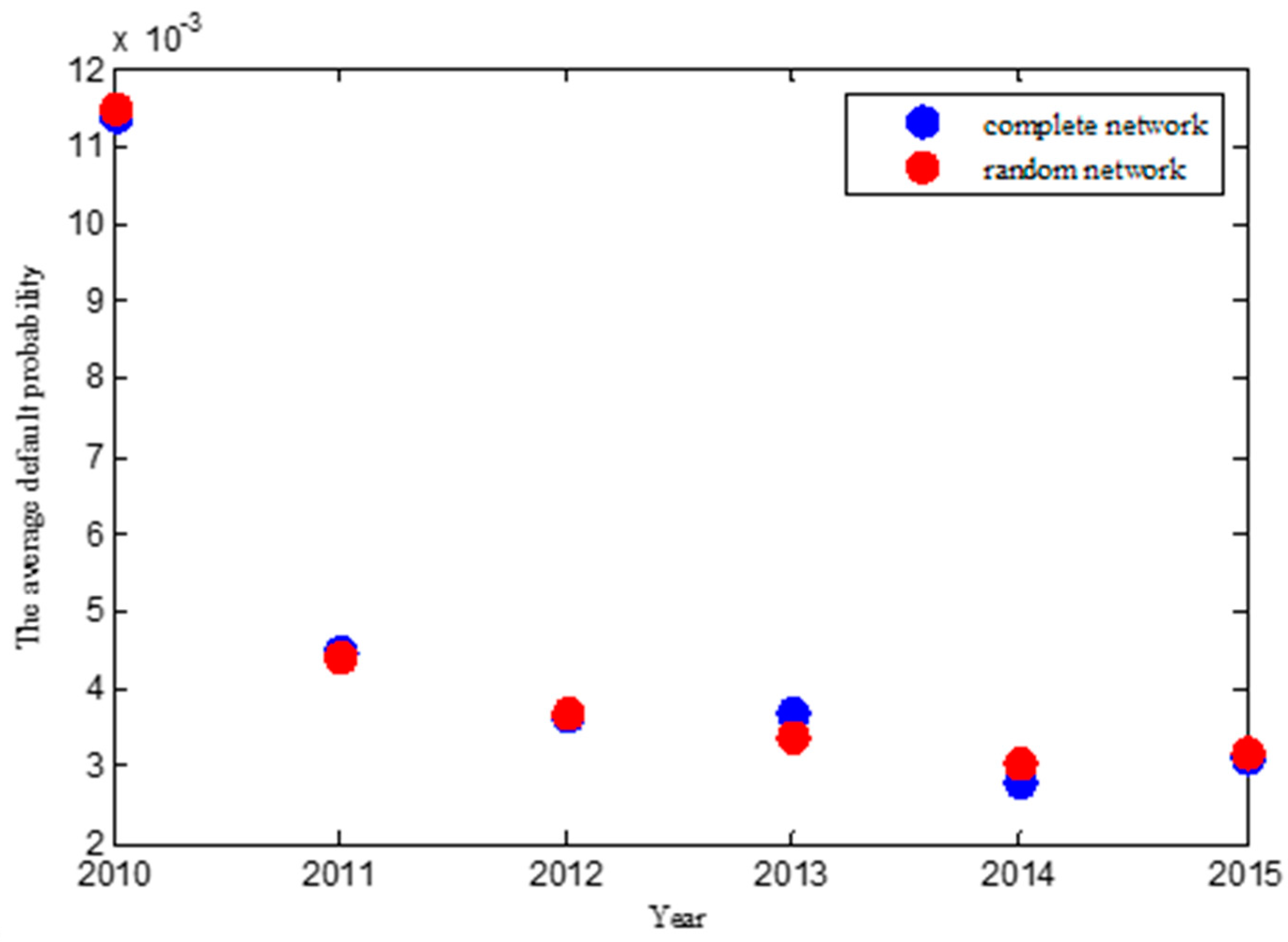
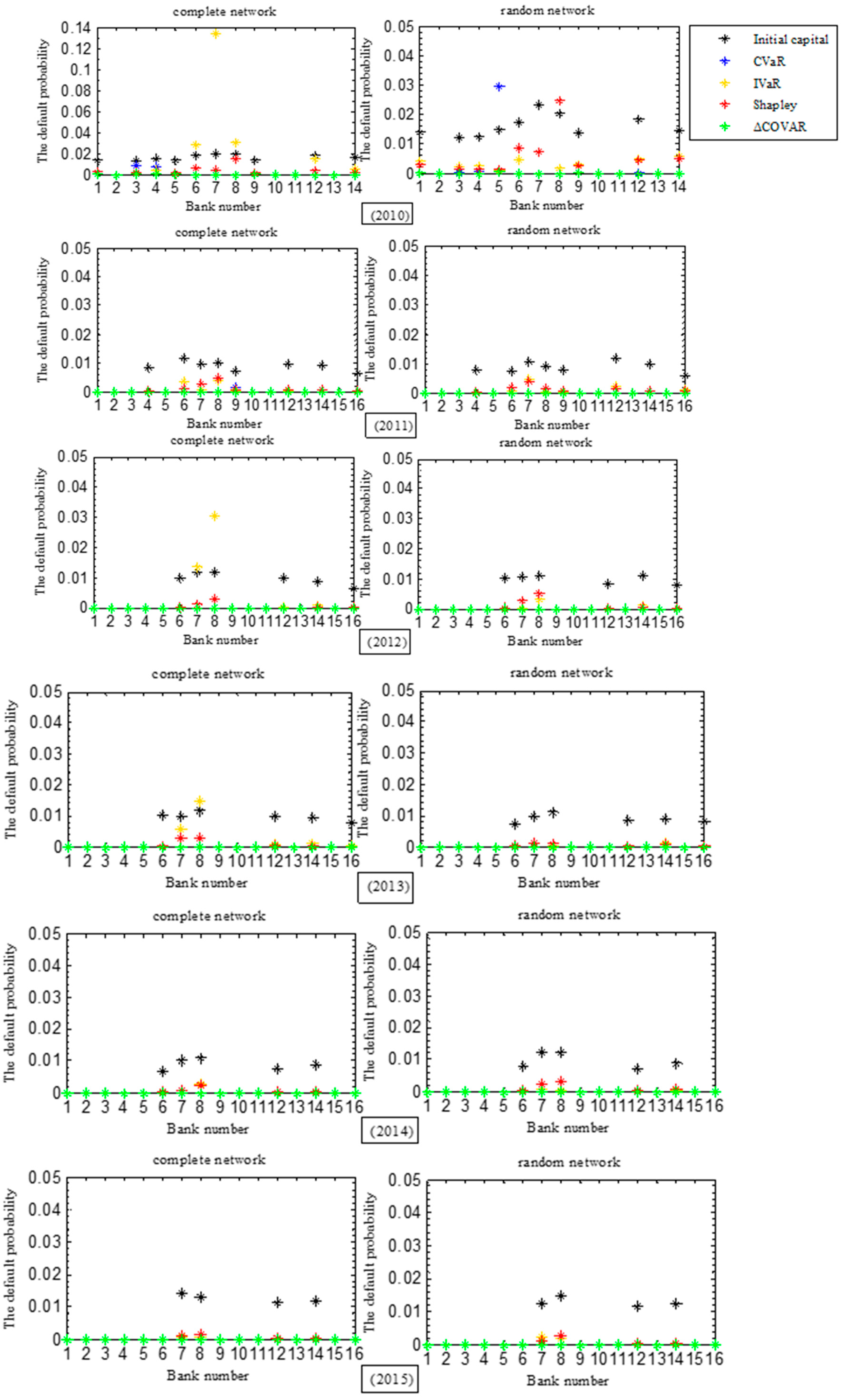
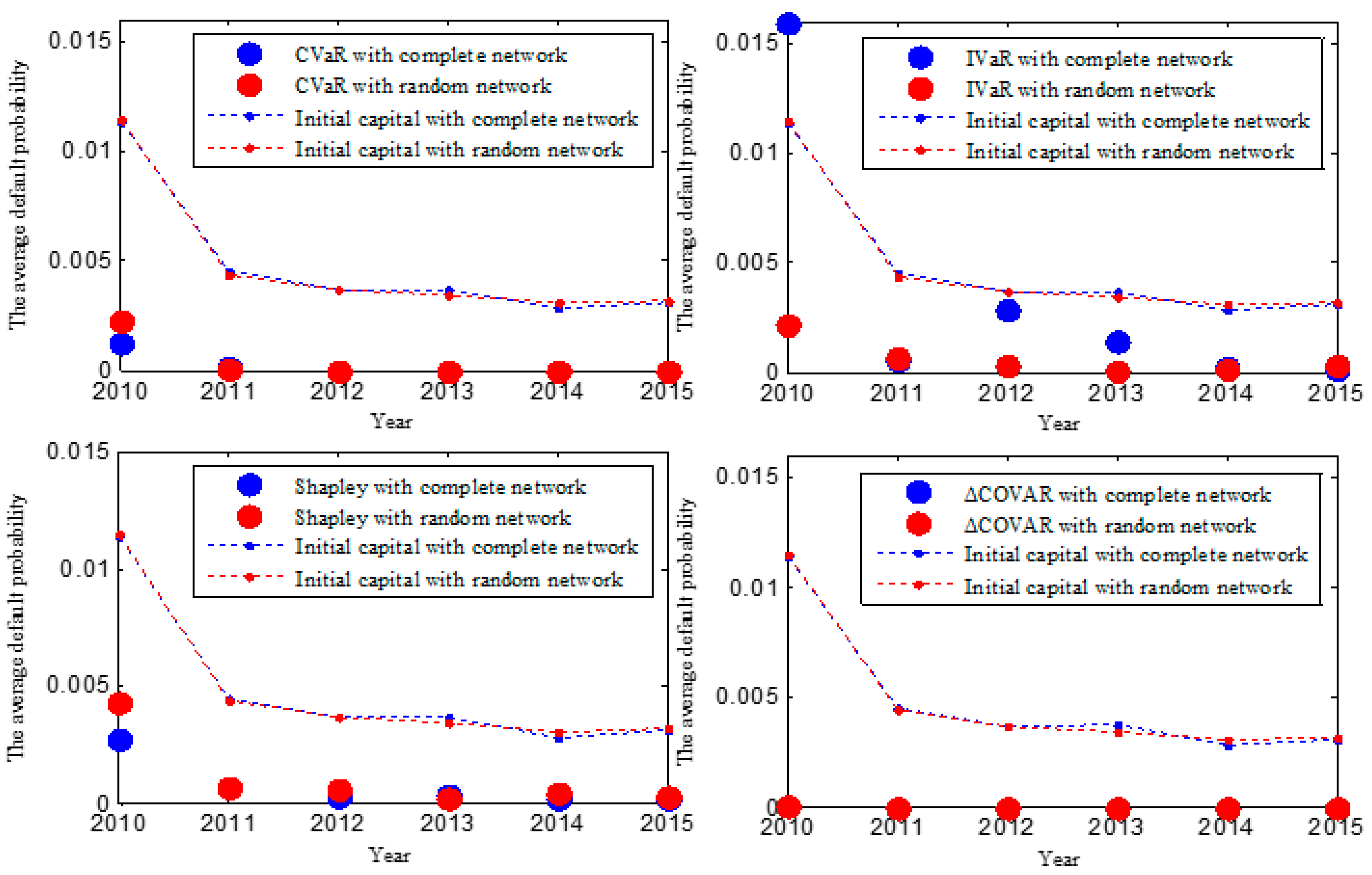
6. Conclusion

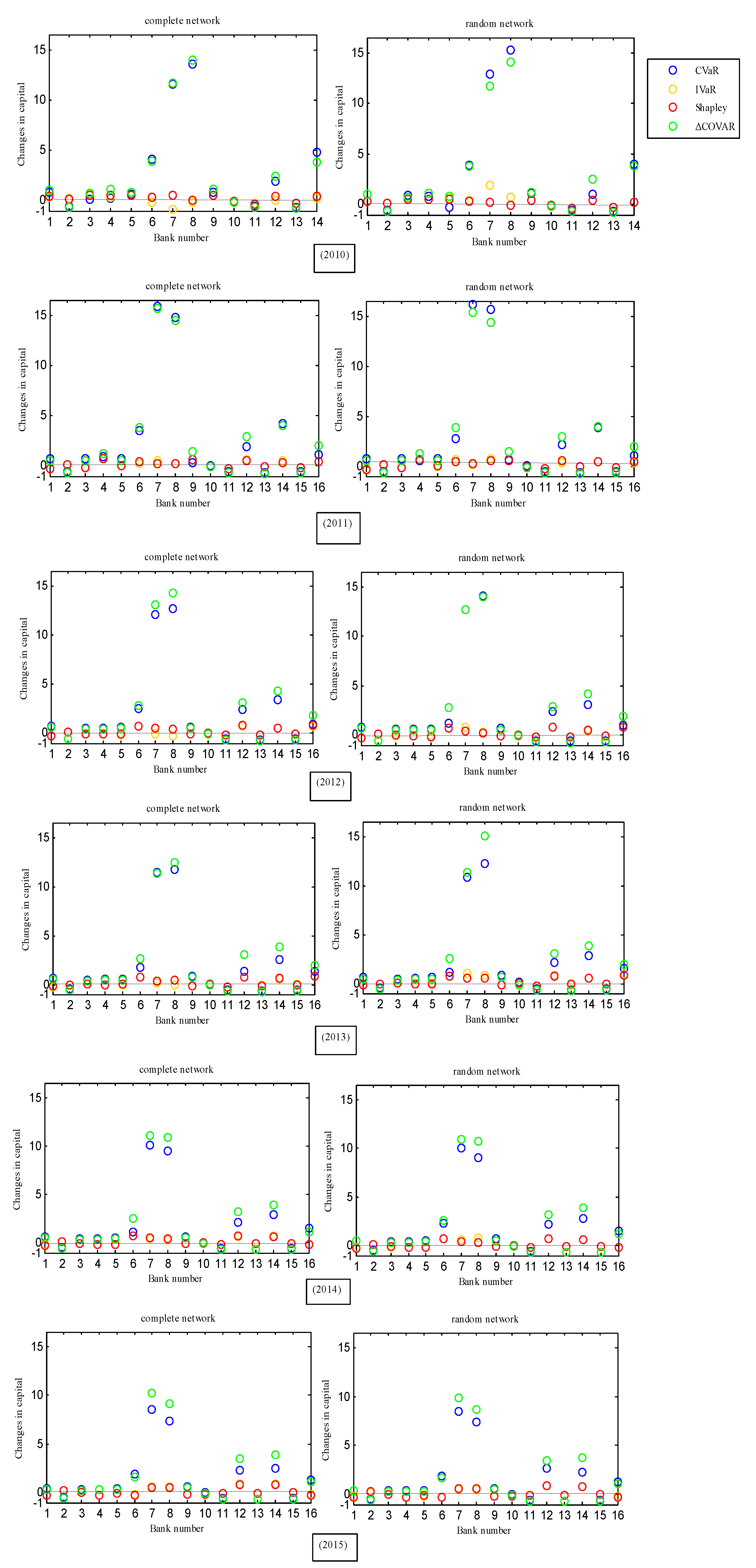
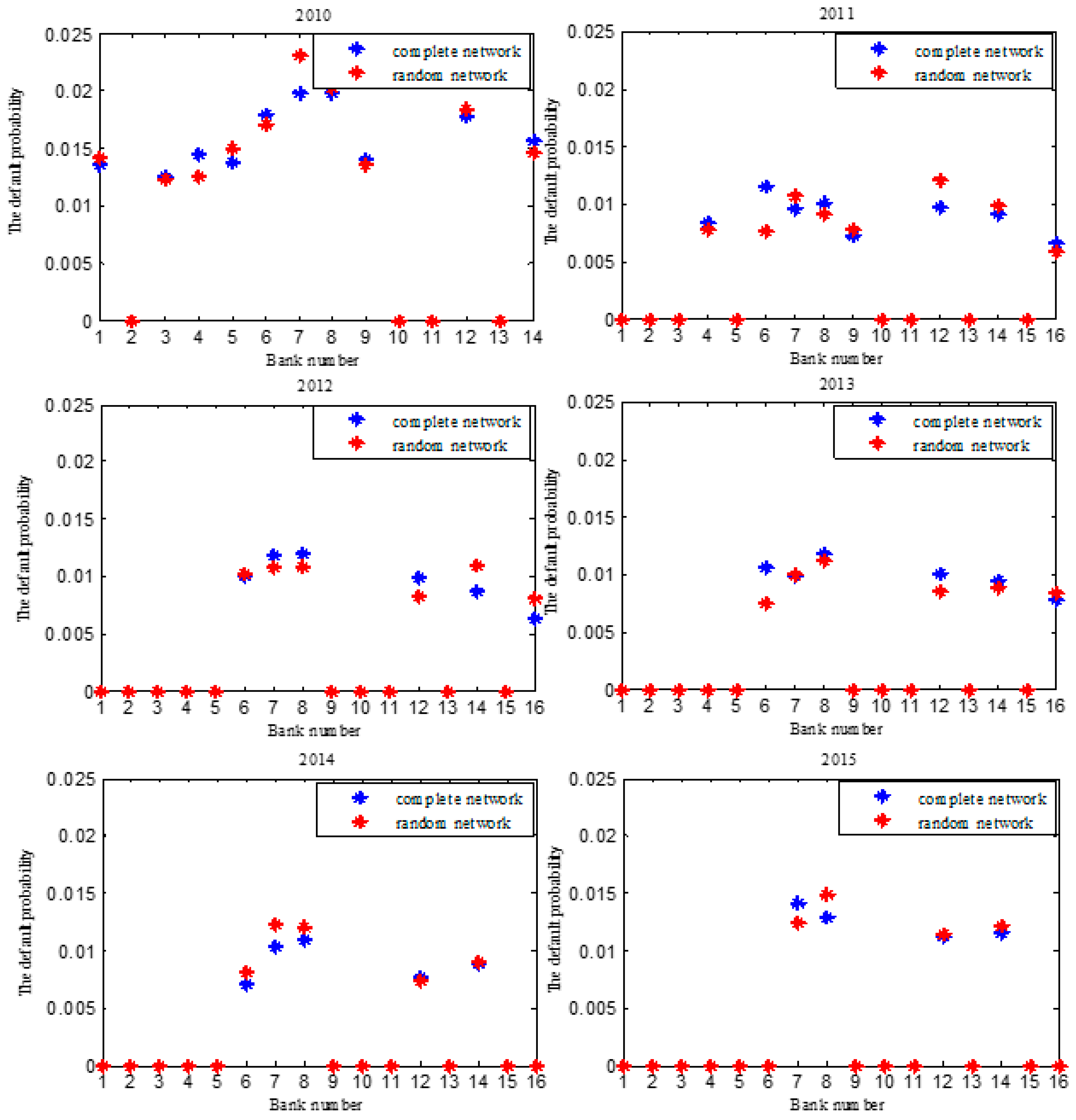
This paper constructed a dynamic model of the Chinese banking network system with complete and random structures and a quantitative macroprudential regulation model using the four risk allocation mechanisms (Component VaR, Incremental VaR, Shapley value EL, and ΔCoVaR). Then we studied empirically the regulation effect by comparing the banks’ default probability. The results show that the default probability of most banks under the four risk allocation mechanisms is significantly lower than that under the initial capital, which indicates that the macro-prudential regulation focus on capital requirements is effective in improving the stability of the banking system. Moreover, it is found that the Chinese banking system with a random network was more stable under the Incremental VaR mechanism in the most years, and the stability of the banking system with the two networks is basically the same under the ΔCoVaR mechanism. Furthermore, the changes in banks’ capital under the Component VaR and ΔCoVaR mechanisms were large in the two networks, while it was relatively small under the other two mechanisms. The regulation effect of the ΔCoVaR mechanism is the most significant. It has strong applicability because it is not affected by the two network structures. The next are Component VaR and Shapley value EL mechanisms. The last is the Incremental VaR mechanism, and the network structure can easily influence it. Lastly, it was found that the four risk allocation mechanisms are essentially allocating the large banks’ surplus capital to those relatively weak banks that are lacking capital. Therefore, the regulators need to set up different capital for each bank based on its contribution to systemic risk in order to ensure the stability of the banking system as a whole.

The present paper enriches the quantitative research on the macroprudential regulation for the Chinese banking system from the perspective of the network structure and provides a certain reference for the relevant financial regulatory agencies. In the future study, we will collect more banks’ actual data to enrich our present study and consider the other network structures.