Optimal Management of a Hybrid Renewable Energy System Coupled with a Membrane Bioreactor Using Enviro-Economic and Power Pinch Analyses for Sustainable Climate Change Adaption

Abstract

This study proposed an optimal hybrid renewable energy system (HRES) to sustainably meet the dynamic electricity demand of a membrane bioreactor. The model-based HRES consists of solar photovoltaic panels, wind turbines, and battery banks with grid connectivity. Three scenarios, 101 sub-scenarios, and three management cases were defined to optimally design the system using a novel dual-scale optimization approach. At the system scale, the power-pinch analysis was applied to minimize both the size of components and the outsourced needed electricity (NE) from Vietnam’s electrical grid. At a local-scale, economic and environmental models were integrated, and the system was graphically optimized using a novel objective function, combined enviro-economic costs (CEECs). The results showed that the optimal CEECs were $850,710/year, $1,030,628/year, and $1,693,476/year for the management cases under good, moderate, and unhealthy air qualities, respectively. The smallest CEEC was obtained when 47% of the demand load of the membrane bioreactor was met using the HRES and the rest was supplied by the grid, resulting in 6,800,769 kg/year of CO₂ emissions.

1. Introduction

Much research has been devoted to tackling contemporary problems including global warming, climate change, environmental pollution, and sustainable development. Sustainable development establishes a basis on which the future world can be built. Hence, a sustainable system may be regarded as a cost-efficient, reliable, and environment-friendly system, which effectively utilizes local resources [1]. Many countries, including developing nations such as Vietnam, should set sustainable development strategies such as an optimal energy management to mitigate climate change impacts, and minimize environmental pollution by application of green energy sources [2,3].

Vietnam enjoys a variety of renewable energy sources such as hydro, solar, wind, biomass, geothermal, and wave energies, along with other Southeast Asian countries. However, few RES projects have been implemented to date, and less than 5.8% of the country’s annual electrical demand was met using small hydropower, and renewables in 2017 [4,5]. Due to rapid economic development, urbanization, industrialization, and population growth, Vietnam’s energy demand is anticipated to increase by 11–16% in the near future. It is also predicted that the rate of increase in energy demand will triple by 2020 [6]. Sustainable energy production is therefore unlikely without the efficient use of renewable energies [7].

Solar and wind energies are two robust RES in developing countries [8,9]. The intermittency problems associated with weather-driven energies could be solved using appropriate storage facilities to minimize the need for grid-sourced electricity [10]. Vietnam enjoys considerable solar radiation and permeant wind flow [4,11]. Several studies have shown that there is a great wind potential in Vietnam, especially in Ninh Thuan and Binh Thuan provinces [5,12,13,14]. The wind speed data used in this study were obtained from the Da Loan station in Lam Dong province at 80 m above sea level, as shown in Figure 1a. Solar energy is the other promising RES in Vietnam. According to the National Center for Hydro-Meteorological Forecasting (NHC), Vietnam has been clustered into three solar regions. The northwestern, and southern regions are mainly and dominantly solar because of a high number of sunshine hours, 1897–2102 h/year, and 1900–2900 h/year, respectively. The central region is moderately solar with fewer sunshine hours, 1400–1700 h/year. Regions with at least 1800 h/year of sunny skies are determined to be appropriate for solar power harnessing [4]. In this study, data from the Song Binh station in Binh Thuan province were used, as shown in Figure 1b.

Vietnam has undergone rapid economic development, abrupt urbanization, extensive industrialization, and fast population growth compared to other developing countries. Thus, environmental pollution including water and air sectors have become a serious problem in this country [15,16]. According to the Environmental Performance Index and the report of the World Bank, the environmental situation in Vietnam was highlighted by several points in 2018. Vietnam ranked 132 among 180 countries in the overall environmental assessment where air pollution index ranked 161. It should be noted that Vietnam was in the top ten countries in the world with the most polluted air [17]. The main reason comes from industrial emissions, coal combustion and increasing numbers of vehicles using non-environmentally friendly fuels [18,19]. Aquatic ecosystems are dangerously threatened by the high amounts of untreated municipal and industrial wastewater discharge from industrial zones [18,19,20]. Thus, effective strategies for environmental protection especially wastewater treatment prior to discharge is vital.

Membrane bioreactor (MBR) technology has many advantages over conventional wastewater treatment plants. MBR technology has less sludge, lower environmental footprint, superior effluent quality, and better intensification, with higher retention time [21]. Properties of the membrane are mainly represented by the membrane module manufacturer. The material, internal and external diameter, surface area, nominal pore size, and tensile strength are described in membrane module properties, and the configuration of modules and available filtration area are detailed in membrane frame properties [22]. In addition, a MBR can be applied in a tropical climate and under the technical and socioeconomic conditions of Vietnam [20]. However, the application of MBRs has been extremely limited in Vietnam because of the high economic costs associated with fouling on the membrane surface. The physicochemical interactions between the membrane and components lead to a decrease in flux and an increase in trans-membrane pressure. This phenomenon increases energy consumption during the pumping process [22,23,24]. Extensive application of MBRs in Vietnam would be both cost-prohibitive and suffer from operational problems. A combination of RES and MBR systems may be a promising sustainable answer to the dilemma [25]. In an RES, selection of an inappropriate size and energy mismanagement in the storage components leads to energy loss and much unmet electrical demand [26]. Hence, an energy management strategy has strongly been recommended for effective utilization and energy loss reduction while meeting the electrical demand [27,28]. However, an optimal management methodology for efficient process integration, one that can meet the dynamic demand load of a MBR using intermittent RES, has yet to be identified.

The aim of the current study was to propose a novel HRES to meet a dynamic demand load of a MBR system under optimum conditions using a dual-scale model. In the first model optimization layer, a power-pinch analysis (PoPA) was used to minimize reliance on the fossil-fuel-dependent power grid of Vietnam. In the second layer, economic and environmental models of the technically optimal energy system were developed to evaluate the performance of the optimal integrated system under three scenarios and 101 sub-scenarios for an optimal management. Subsequently, an optimal management scenario was determined using an enviro-economic model, and the technical and enviro-economic models were employed at two optimization scales.

2. Materials and Methods

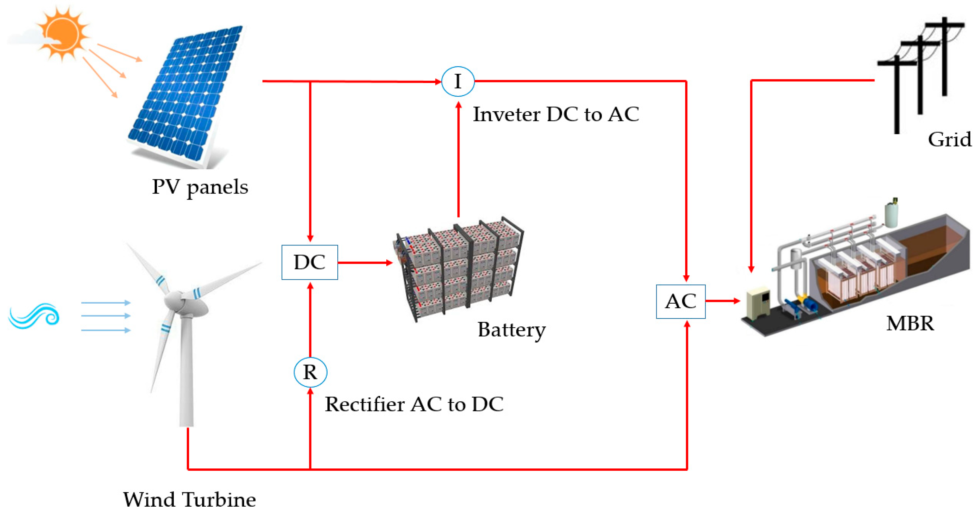
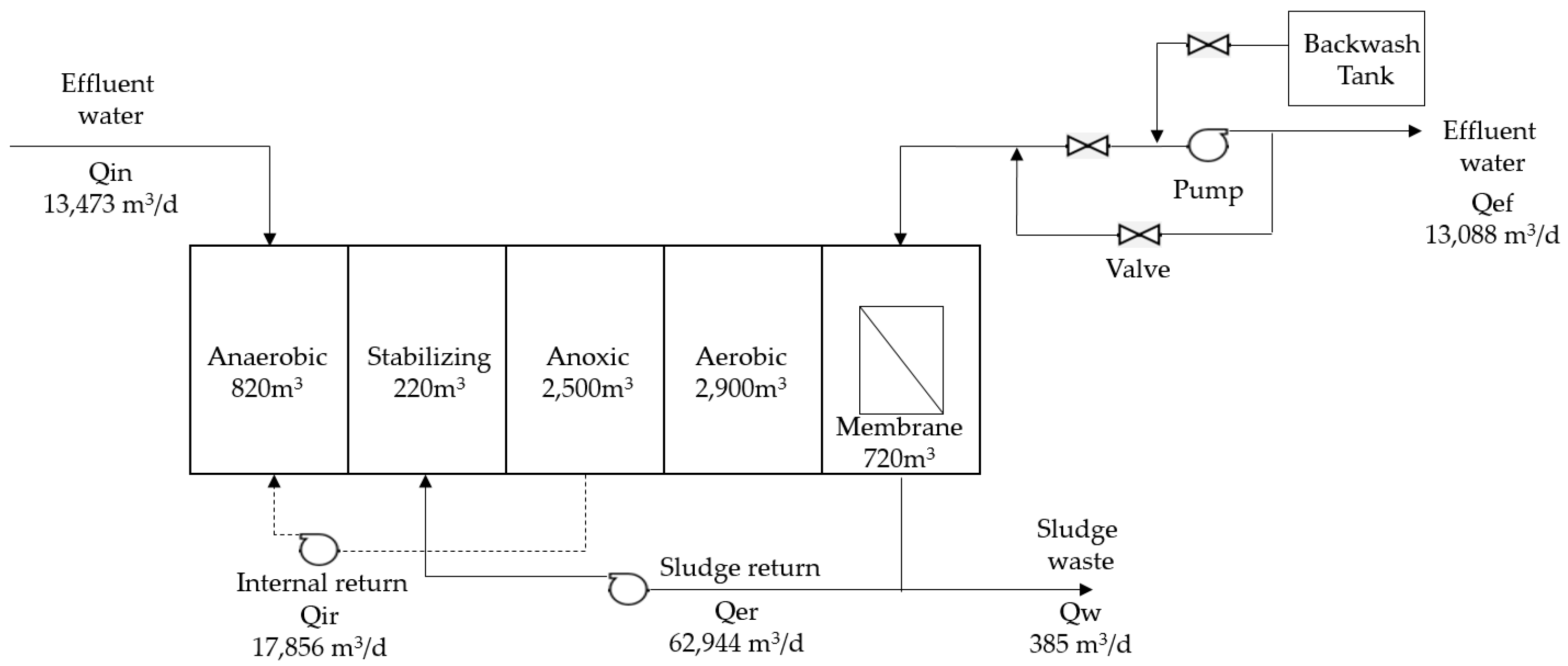
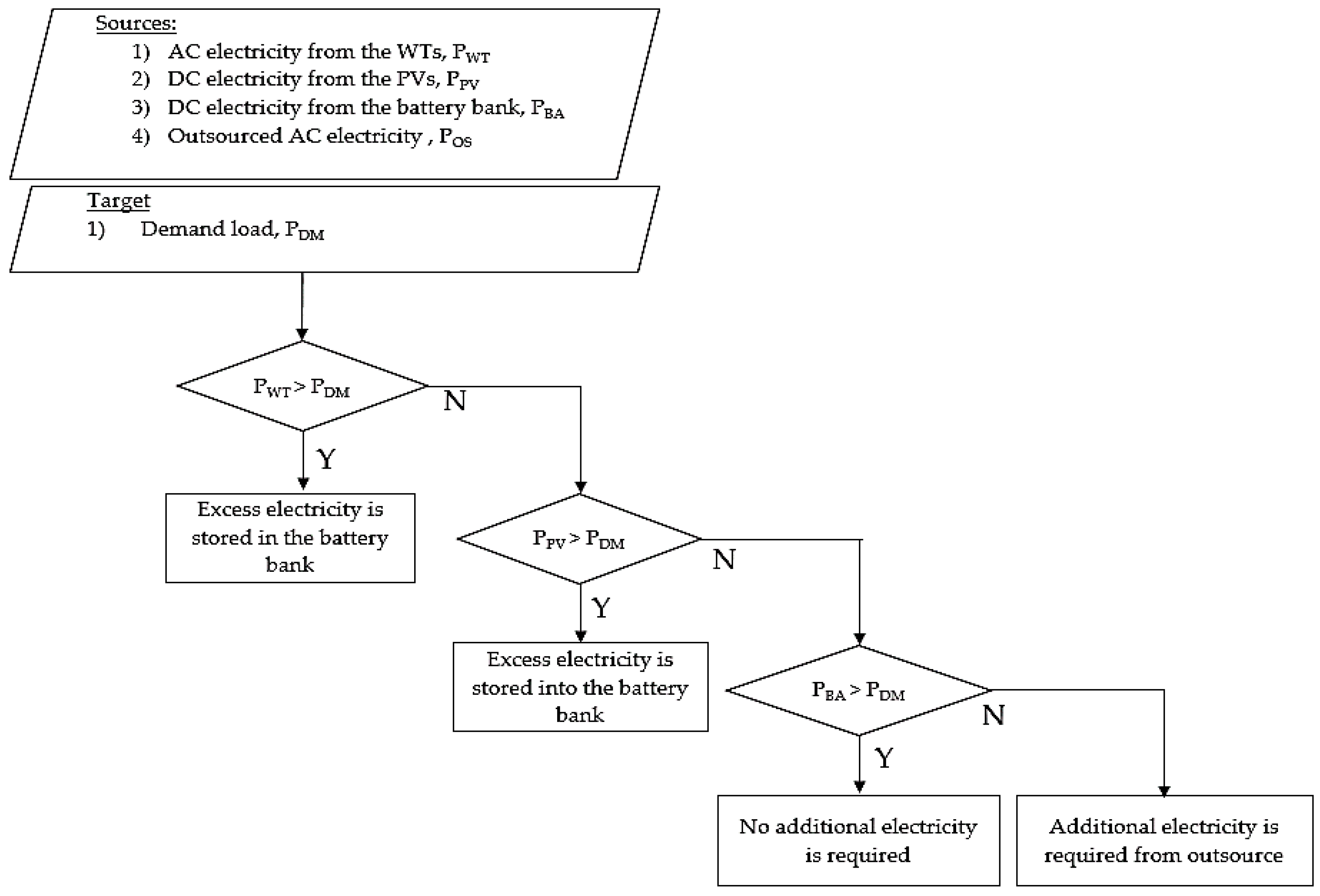
2.1. System Configuration and Energy Management Strategy

A schematic representation of the system under study is shown in Figure 2. Wind turbines generate an alternating current (AC), while photovoltaic panels (PV) generate direct current (DC). Because a MBR with an external supply source operates on AC, an inverter is used to convert electricity from DC (generated by PV panels or stored in a battery bank) to AC before delivering it to the MBR. A rectifier can convert AC electricity generated by wind turbines (WTs) to DC for storage in a battery bank (BB). Three electrical losses were considered: during energy conversion in the PV panels and WTs; during charging and discharging of the battery; and during net AC-to-DC conversion [29].

Figure 3 is a schematic representation of a MBR system. The demand load was obtained from an operating full-scale MBR plant in southern Vietnam. The plant consists of five main basins, including anaerobic, stabilizing, anoxic, aerobic, and a submerged reactor. In the submerged reactor, the membrane module is immerged in the bioreactor. There is no recirculation loop [30]. Thus, a MBR using a submerged reactor has lower energy consumption because of no high pressurizing pump for recirculation [31]. Here, polyvinylidene (PVDF) membrane material was used with the hollow fiber of 0.01 µm diameter because of its acceptable physical and chemical resistance. Volumes of the bioreactors are shown in the figure. The plant’s operating temperature was maintained at 20 °C for cycles of 15 min (14.5 min for filtration, with the remaining time for back-washing).

An optimal energy management approach was proposed to minimize the components’ size in the integrated system as well as the power losses, as illustrated in Figure 4 [28]. According to the figure, AC electricity is generated by the WTs, and consumed to meet the demand load of the MBR. If the generated AC is greater than the MBR demand load in any time interval, excess AC is converted to DC voltage via converters, and then stored in batteries. On the other hand, the DC generated by the PV panels is converted into AC, and delivered to the demand if the demand load is greater than the power generated by AC source. The battery is charged when the generated DC is greater than the demand load and vice versa. Outsourced electricity is imported from the grid if the total electricity in the HRES is not adequate to satisfy the demand load. Power losses were considered in the model to obtain realistic results. The conversion efficiency, charge and discharge efficiency in the lead-acid batteries, and self-discharge ratio were assumed to be 95%, 90%, and 0.004%/h, respectively [28]. However, these values could vary according to operating devices in an in-situ application.

The research framework used to evaluate the optimal configuration is shown in Figure 5. The raw meteorological data were collected, and the optimal configuration was obtained using the analyzed data in various sub-scenarios. An economic assessment was performed on an optimal integrated system to determine the total annual cost (TAC) and the environmental performance of the integrated system considered total annual carbon dioxide emissions (TACO₂) by the grid for all sub-scenarios. Finally, an optimal scenario was determined graphically using the enviro-economic penalty cost. A step-by-step procedure to determine the optimal configuration is detailed as follows:

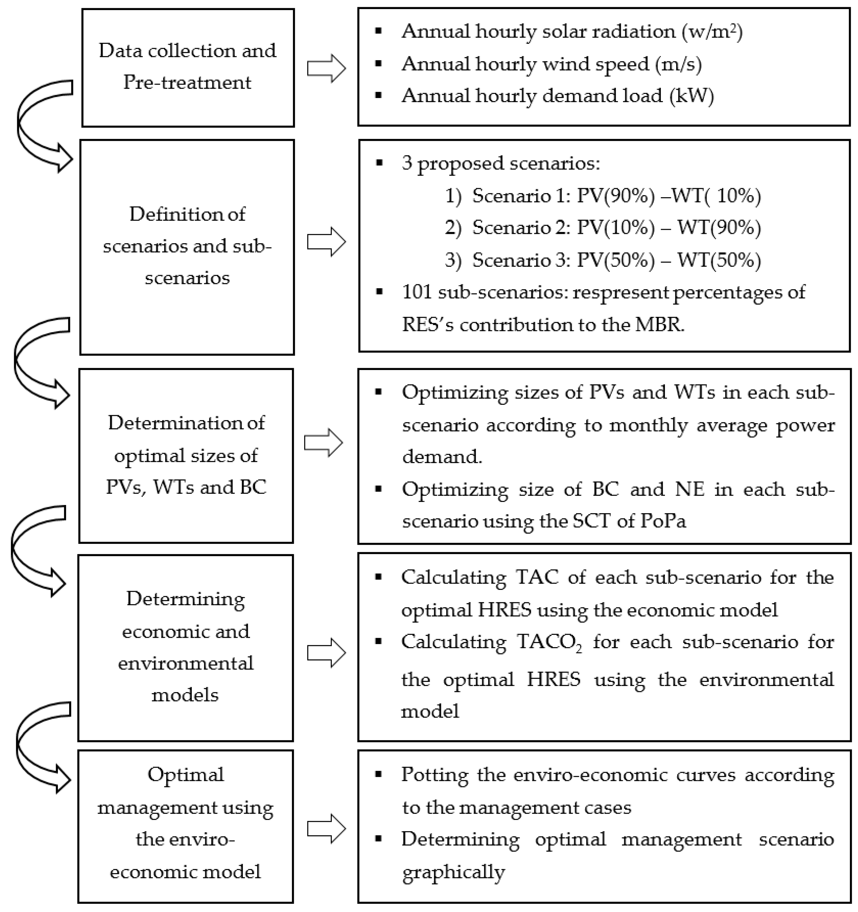
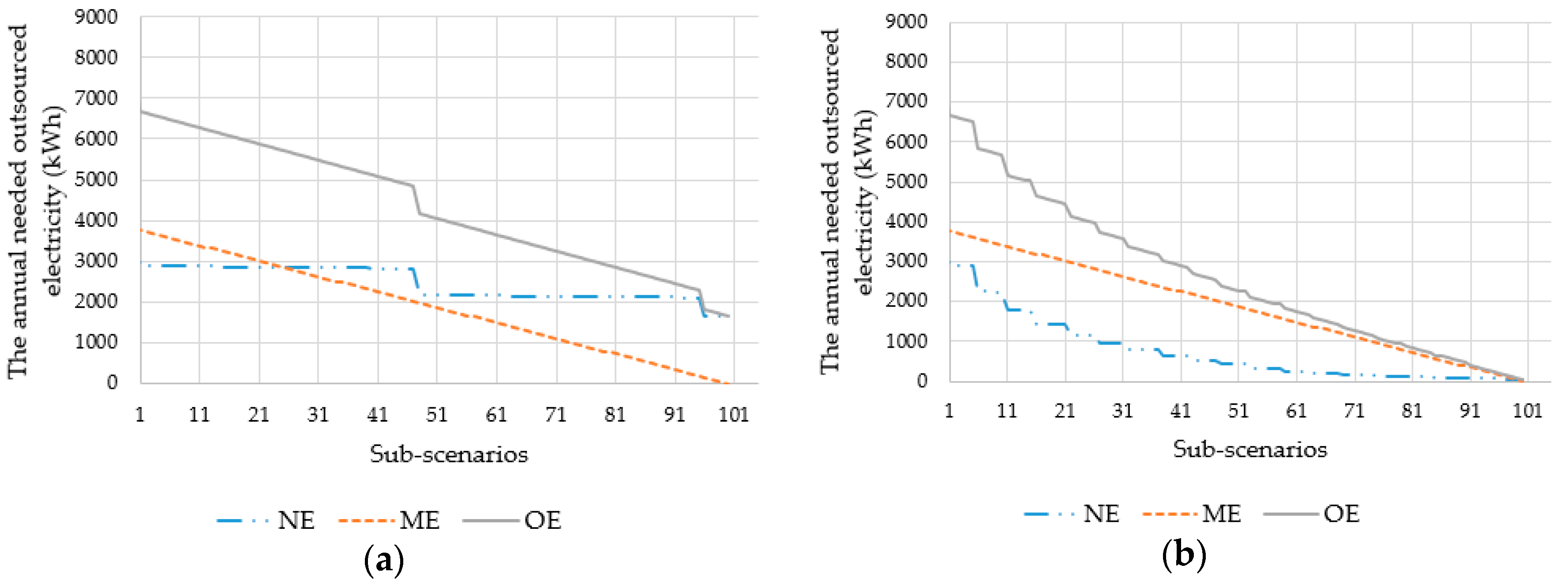
• The optimal numbers of PVs and WTs were determined according to sub-scenarios. This study considered three scenarios and 101 sub-scenarios. The sub-scenarios accounted for the percentage of RES contribution in satisfying the electricity in the MBR so that k% RES contribution was used in the (k + 1)th sub-scenario. The MBR operated without any contribution from the HRES in the first sub-scenario. To consider the individual contributions of each power source in one HRES configuration, three scenarios were assumed:
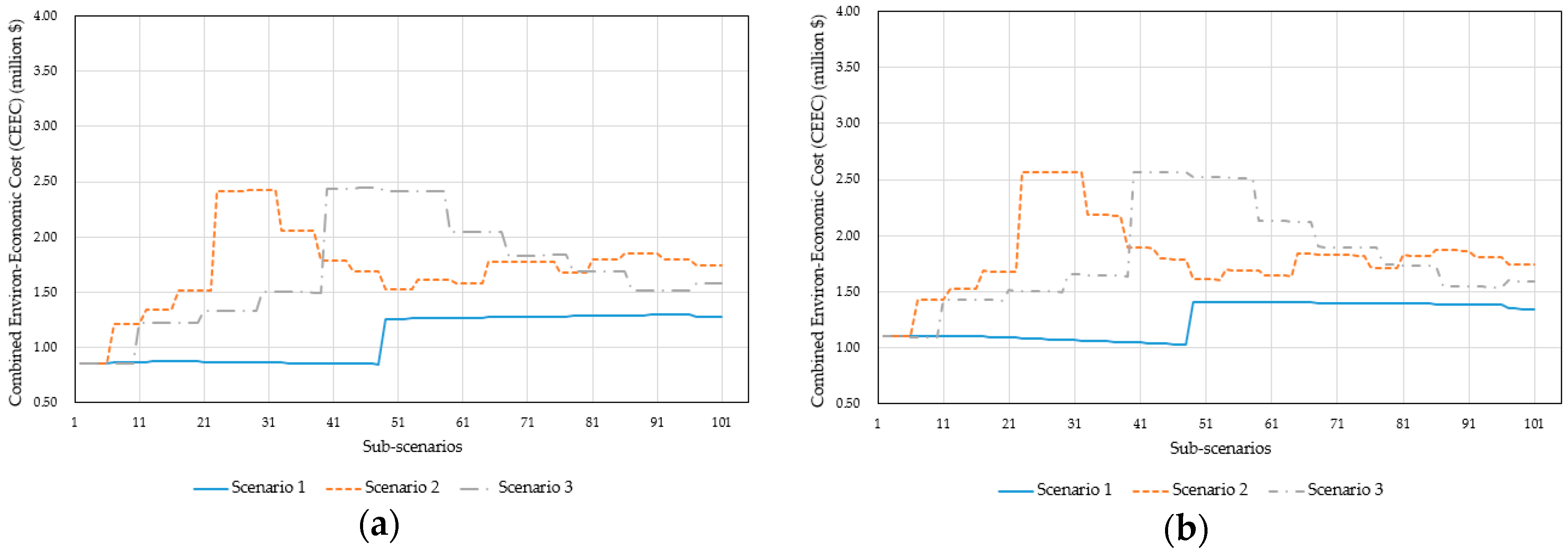
  • Scenario 1: The solar (DC) source accounts for 90% of the total amount provided by the RES, while the wind energy (AC) source makes up the remaining 10%. This scenario is suitable for locations where the potential of solar energy source is dominant compared to that of wind energy source.
  • Scenario 2: The wind (AC) source accounts for 90% of the total amount provided by RES, whereas the solar (DC) source makes up the remaining 10%. This scenario should be considered in regions where the wind energy source has higher priority compared to solar energy sources.
  • Scenario 3: The wind (AC) and solar (DC) sources contribute equally. In other words, each supplies 50% of the total amount provided by the RES. Here, the potential of both wind and solar energies is highly recommended.
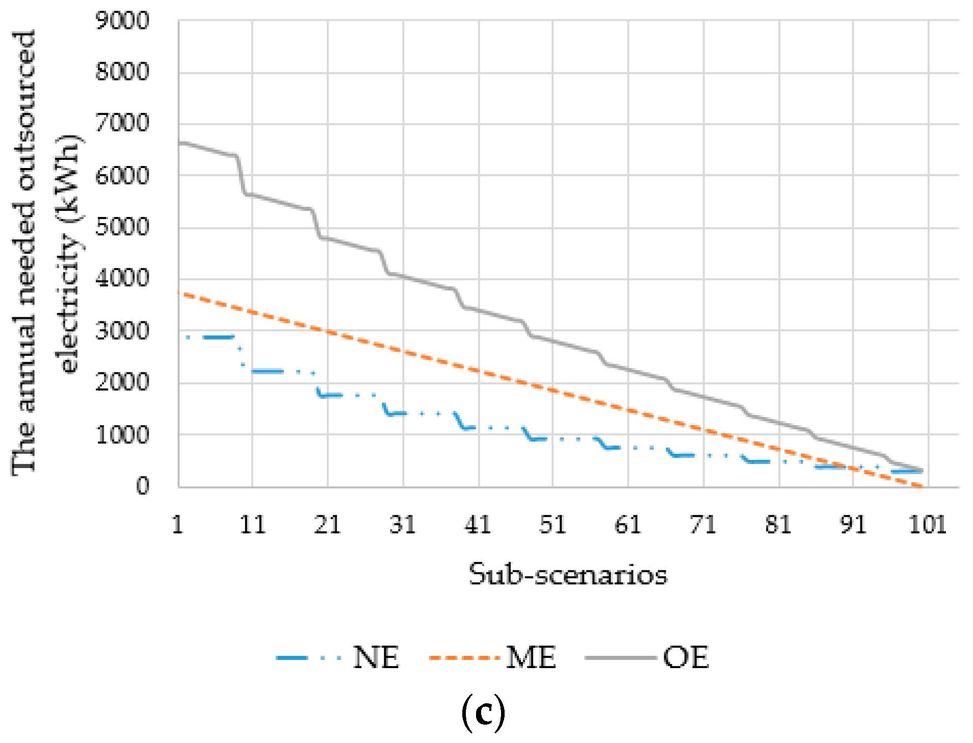
  The representative of these three scenarios has the individual contribution in each RES source. This could give us an idea to select an appropriate source based on a specific location.
• An appropriate battery capacity (BC) and the outsourced needed electricity (NE) for one operational year were determined for each sub-scenario using the storage cascade table (SCT) of PoPA [29].
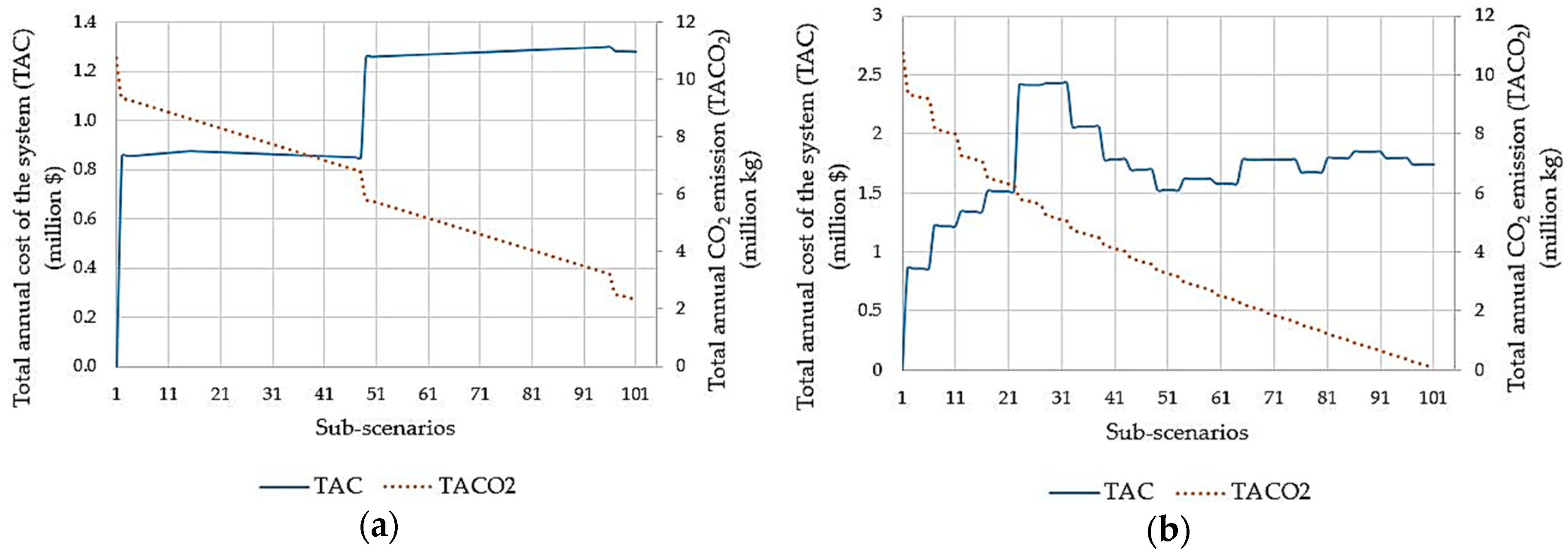
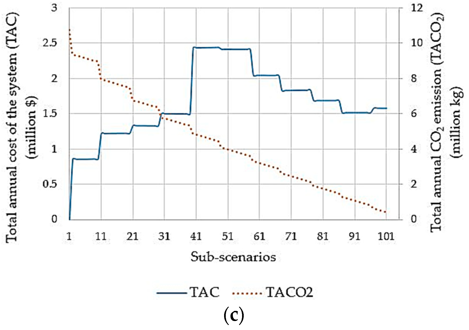
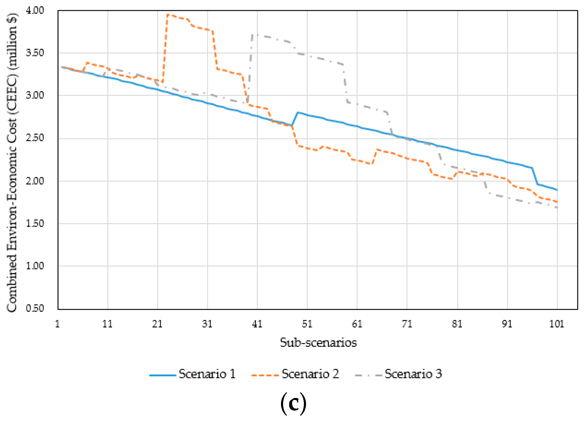
• Curves of the combined economic and environmental penalty costs (CEEPC) were plotted using economic and environmental models for all sub-scenarios in three management cases, and the optimal sub-scenario was determined graphically.

2.2. Data Collection

Solar and wind are known as weather-driven energy sources because of their dependency on the structure of raw meteorological data [9]. Furthermore, the demand load has a dynamic pattern determined by the performance of the MBR.

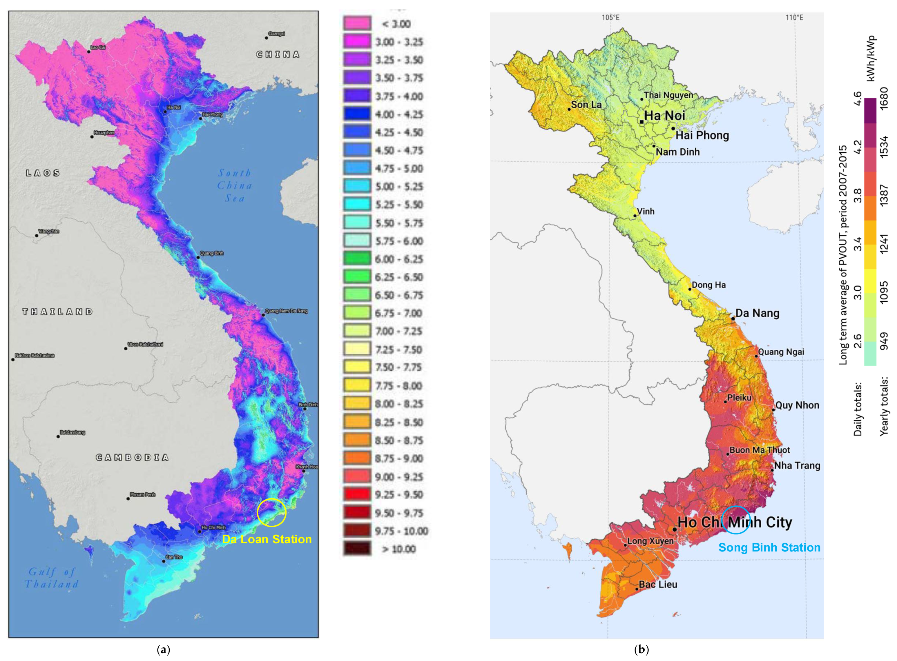
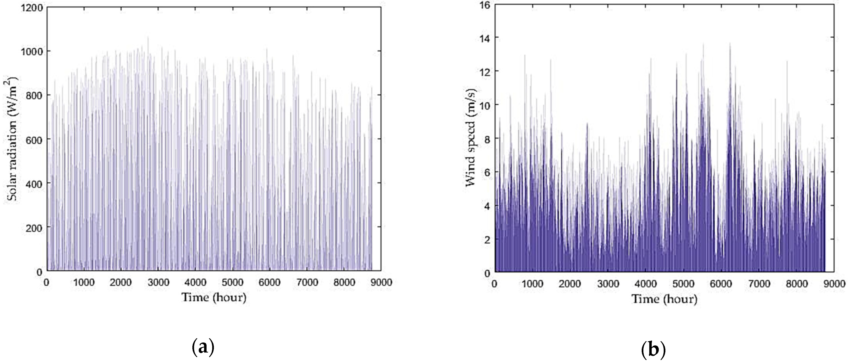
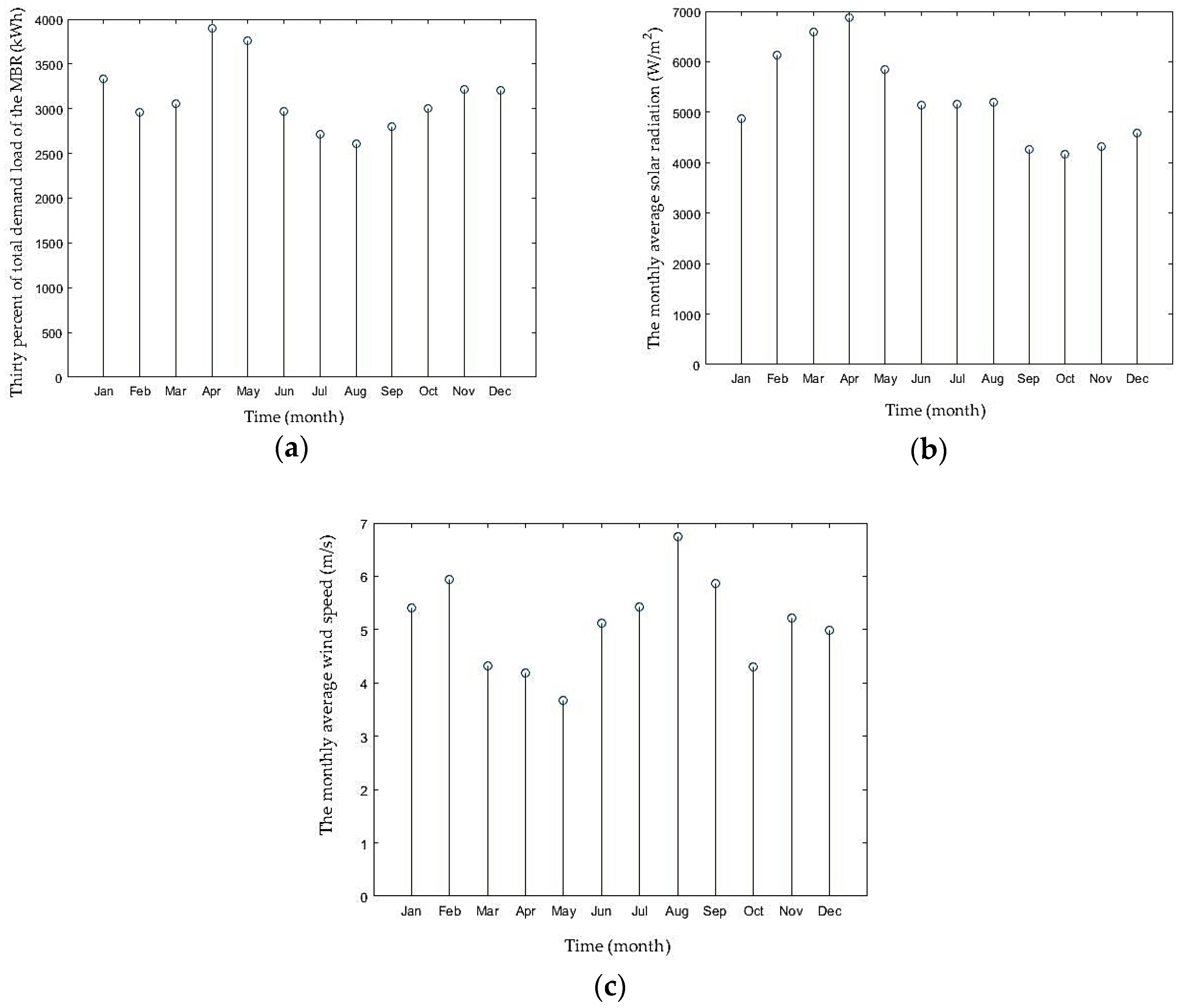
2.2.1. Solar Radiation and Wind Speed Data

Solar radiation and wind speed data were extracted from Energy Data website, an open platform providing access to energy datasets and data analytics [32]. Wind speed measurements were performed at the Da Loan station in Lam Dong Province in Vietnam using the “Wind measurement for developing wind power plan and wind power project”, which is financed by the German Federal Ministry of Environment, Nature Conservation and Nuclear Safety, and the Vietnam Ministry of Industry and Trade. Wind speed data were collected at an anemometer height of 80 m above sea level for one full year. The data were processed by high-quality sensor technology, based on the current international standard IEC 61400-121 [33]. Solar radiation data were obtained from the Song Binh station in Binh Thuan Province, Vietnam, from a project funded by the Energy Sector Management Assistance Program. Solar radiation and wind speed hourly data are presented in the Supplementary Materials and shown graphically in Figure 6. Solar irradiance meets 1 kWh/m² at peak time intervals and varies mainly between 400 and 500 W/m² in sunny hours. Wind speed data fluctuate because of the site’s topography. Wind speeds rarely exceed 12 m/s and usually fluctuate between 2 and 8 m/s.

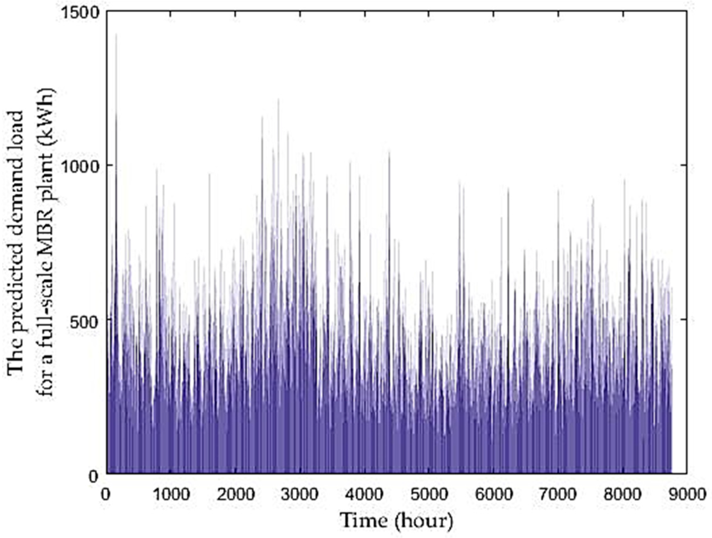
2.2.2. Demand Load of MBR

The energy consumption of the MBR was calculated according to influent and effluent qualities, while flow rates were obtained from a real MBR plant in Vietnam. The demand load of the MBR plant was the sum of the energy consumption in all processes. Only aerating ($AeE$), pumping sludge ($Pu{E}_{slu}$), pumping permeate ($Pu{E}_{per}$), and mixing was assumed in required bioreactors ($MiE$). According to the Benchmark Model No. 1, the electricity demand of aeration, pumping, and mixing processes can be calculated using Equations (1)–(4) [34].

$$AeE=\frac{S_O^{Sat}}{\left(t_1-t_0\right)\times 1.8\times 1000}{\displaystyle \underset{t_0}{\overset{t_1}{\int }}{\displaystyle \sum _{i=1}^5{V}_i}}\times K_L{a}_i(t)\times dt,$$

(1)

$$Pu{E}_{slu}=\frac{1}{t_1-t_0}{\displaystyle \underset{t_0}{\overset{t_1}{\int }}\left(0.004\times Q_{ir}(t)+0.008\times Q_{er}(t)+0.05\times Q_w(t)\right)}\times dt,$$

(2)

$$Pu{E}_{per}=\frac{1}{t_1-t_0}{\displaystyle \underset{t_0}{\overset{t_1}{\int }}\frac{\Delta P{Q}_{ef}(t)}{3600\eta }}dt,$$

(3)

$$\begin{array}{c}MiE=\frac{24}{t_o}{\displaystyle \underset{t_0}{\overset{t_1}{\int }}{\displaystyle \sum _{i=1}^5\left(0.005\times V_i\right)}\times }dt \mathrm{if} K_L{a}_i(t)<20{\mathrm{d}}^{-1},\\ MiE=0 \mathrm{if} \mathrm{otherwise},\end{array}$$

(4)

where $t_0$ and $t_1$ are the first and last hours of observation (h), respectively; $S_O^{Sat}$ is the saturated concentration of the dissolved oxygen in water (g/m³); $V_i$ is the volume of the ith bioreactor (m³); $K_L{a}_i(t)$ is the oxygen transfer coefficient of the ith bioreactor at time t (h⁻¹); $Q_{ir}(t)$, $Q_{er}(t)$, $Q_w(t)$, and $Q_{ef}(t)$ are the flow rates of the returned sludge from the anoxic to anaerobic bioreactor, the returned sludge from the membrane to stabilizing bioreactor, waste sludge from the membrane bioreactor to a target waste treatment system, and effluent discharging from MBR to sinks in m³/h, respectively; $\Delta P$ is the trans-membrane pressure; and $\eta$ is the permeate pump efficiency.

The hourly demand load of the MBR plant is given in the Supplementary Materials and displayed graphically in Figure 7. The plant’s electrical demand load varies between 300 and 500 kW and reaches 1.4 MW at peak demand.

2.3. Optimal Configuration

A numerical tool of PoPA, known as a storage cascade table (SCT), was employed to determine two energy targets, the minimum outsourced electricity supply (MOES) and the available excess electricity for the next day (AEEND) in each operating day during one year [29]. The minimum NE and the optimal BC were then determined. The following simplifying assumptions were considered for the in-silico model development [35,36].

• The intensity of diffuse sky radiation is uniform over the sky dome, and dust and dirt accumulation is neglected on photovoltaic panels.
• The effects of the wind velocity on the PV cell performance have not been considered.
• The power losses in the system were considered as reduction factors in the models.
• The uncertainties in the power market has been neglected.

The SCT was constructed and applied to determine the energy targets. The sub-scenario in which the RES supplied 30% of the total demand load on the second day of operation was used to detail SCT construction. This detailed sub-scenario (the 31st) is categorized under Scenario 2. Wind accounted for 90% of the RES, and solar supplied the rest in the detailed sub-scenario [29]. The SCT table (

Table 1. Storage cascade table.

1	2	3	4	5	6	7	8	9	10	11	12	13	14	15
Time (h)	Time Interval (h)	DC Source, ${\mathit{P}}_{\mathit{P}\mathit{V}}$ (kWh)	AC Source, ${\mathit{P}}_{\mathit{W}\mathit{T}}$ (kWh)	AC Demand, ${\mathit{P}}_{\mathit{D}\mathit{M}}$ (kWh)	Additional Amount from DC Source (kWh)	Second Additional Amount Required from the Battery (kWh)	AC Surplus (kWh)	DC Surplus (kWh)	Charging into Battery, $\mathit{I}\mathit{N}$ (kWh)	Discharging from the Battery, $\mathit{O}\mathit{U}\mathit{T}$ (kWh)	Infeasible Storage Capacity, $\mathit{I}\mathit{S}\mathit{C}$ (kWh)	Infeasible Outsource Electricity, $\mathit{I}\mathit{O}\mathit{E}$ (kWh)	Feasible Storage Capacity, $\mathit{F}\mathit{S}\mathit{C}$ (kWh)	Feasible Outsource Electricity, $\mathit{F}\mathit{O}\mathit{E}$ (kWh)
													1184.19	2267.37
1	1	0	226.17	631.06	404.88	404.88	0	0	0	426.19	0.00	404.88	710.59	0
2	1	0	388.52	350.10	0	0	388.52	0	369.09	0	332.18	0	1042.75	0
3	1	0	424.17	463.54	39.36	39.36	0	0	0	41.44	286.13	0	996.66	0
4	1	0	424.17	461.18	37.01	37.01	0	0	0	38.96	242.83	0	953.34	0
5	1	0	380.87	395.44	14.57	14.57	0	0	0	15.34	225.78	0	936.26	0
6	1	0.08	309.88	291.87	0	0	309.88	0.08	294.47	0	490.79	0	1201.25	0
7	1	0.32	293.63	270.41	0	0	293.63	0.32	279.27	0	742.12	0	1452.54	0
8	1	0.66	337.11	391.88	54.77	54.14	0	0	0	56.99	678.77	0	1389.17	0
9	1	1.19	54.05	343.57	289.52	288.39	0	0	0	303.56	341.45	0	1051.82	0
10	1	0.87	19.62	323.64	304.02	303.19	0	0	0	319.15	0	11.26	697.17	0
11	1	1.22	63.89	376.11	312.22	311.06	0	0	0	327.43	0	311.06	333.32	0
12	1	1.67	49.05	638.23	589.18	587.60	0	0	0	618.53	0	587.60	0	587.60
13	1	1.68	242.65	447.09	204.44	202.85	0	0	0	213.52	0	202.85	0	202.85
14	1	1.57	123.88	590.05	466.17	464.68	0	0	0	489.13	0	464.68	0	464.68
15	1	1.02	256.98	542.01	285.03	284.06	0	0	0	299.01	0	284.06	0	284.06
16	1	0.54	534.53	437.50	0	0	534.53	0.54	508.34	0	457.50	0	457.50	0
17	1	0.05	424.17	524.36	100.18	100.14	0	0	0.0	105.41	340.36	0	340.36	0
18	1	0	828.47	498.33	0	0	828.47	0	787.04	0	1048.69	0	1048.69	0
19	1	0	646.20	397.84	0	0	646.20	0	613.89	0	1601.14	0	1601.14	0
20	1	0	640.81	583.59	0	0	640.81	0	608.77	0	2148.97	0	2148.97	0
21	1	0	300.06	662.95	362.89	362.89	0	0	0	381.98	1724.46	0	1724.46	0
22	1	0	603.95	616.93	12.98	12.98	0	0	0	13.66	1709.21	0	1709.21	0
23	1	0	354.91	419.38	64.46	64.46	0	0	0	67.86	1633.74	0	1633.74	0
24	1	0	148.71	532.99	384.27	384.27	0	0	0	404.50	1184.24	0	1184.24	0

) was constructed as detailed as follows.

• Operation hours are given in Column 1 that are listed from “1 h” to “24 h” in a daily pattern. Time intervals are the durations between two adjacent operation hours given in Column 2.
• Hourly DC and AC electricity are measured in kWh, and given in Columns 3 and 4, respectively, calculated using Equations (5) and (6) [37,38].

  $$P_{PV}=A_1\times {\eta }_1\times P_f\times {\eta }_{pc}\times I\times n_1,$$

  (5)

  $$P_{WT}=0.5\times C_p\times \rho \times A_2\times v^3\times n_2,$$

  (6)

  where $P_{PV}$ is the direct current produced by PV panels, $A_1$ is the area of the PV panel with a unit area of 1.63 m²/kWh, ${\eta }_1$ is the efficiency of the module (0.11), $P_f$ is the packing factor assumed to be 0.9, ${\eta }_{pc}$ is the power conditioning efficiency assumed to be 0.86, $I$ is the solar radiation (W/m²), $n_1$ is the number of PV panels in a solar module, $P_{WT}$ is the produced power by the WTs ( kWh), $C_p$ is the wind turbine’s power coefficient assumed to be 0.5, $\rho$ is the ambient air density considered as 1.225 kg/m³, $v$ is the wind speed in m/s, $n_2$ is the number of WTs in a wind farm, and $A_2$ is the swept area by the turbine blades that have rotor radius $r$, which is obtained via Equation (7) [38].

  $$A_2=\pi \times r^2,$$

  (7)
• The hourly AC electricity demand of the MBR system ($P_{DM}$) is given in Column 5 in kWh.
• If the AC electricity is not adequate to meet the demand load at any time intervals, the DC electricity is delivered. The required power is obtained using Equation (8) that is given in Column 6 [29].

  $$Additional amount from the DC source=P_{DM}-P_{WT},$$

  (8)
• The battery is discharged when the total AC and DC electricity is not enough to meet the demand load, the required amount of battery power is obtained using Equation (9). The calculated quantities are given in Column 7 [29].

  $$Second additional amount required from the battery=P_{DM}-P_{WT}-P_{PV}\times c,$$

  (9)

  where $c$ is the conversion efficiency (0.95).
• The battery is charged when the generated DC and AC electricity is greater than the MBR demand load. The amounts of surplus AC and DC power are, respectively, summarized in Columns 8 and 9. The charged ($IN$) and discharged ($OUT$) power quantities are, respectively, calculated according to Columns 8 and 9, and Column 7. The $IN$ and $OUT$ are obtained using Equations (10) and (11) and listed in Columns 10 and 11, respectively [29].

  $$IN=ACsurplus\times ch+DCsurplus,$$

  (10)

  $$OUT=Second additional amount from the battery/ch,$$

  (11)

  where $ch$ is charge/discharge efficiency (0.95).
• The maximum electricity storage capacity for the battery ($BC$) and the outsourced electricity requirement at various time intervals were obtained by cascading the quantities of storage capacity and outsourced electricity columns, respectively. Infeasible storage capacity ($ISC$) and infeasible outsourced electricity ($IOE$) that represented the first day of operation are obtained using Equations (12) and (13) and given in Columns 12 and 13, respectively [29]. Feasible storage capacity (FSC) and feasible outsourced electricity (FOE) that represented a normal day of operation are obtained using Equations (14) and (15) and given in Columns 14 and 15, respectively [29]. Here, only the second day of operation was described as a normal day of operation for simplicity.

  $$IS{C}_j^1=IS{C}_{j-1}^1\times \left(1-s\right)+I{N}_j^1\times c-OU{T}_j^1/c,$$

  (12)

  $$IO{E}_j^1=-IS{C}_j^1\times \left(ch\times c\right) ,$$

  (13)

  $$\begin{array}{c}FS{C}_j^i=IS{C}_{24}^1+FS{C}_{j-1}^i\times \left(1-s\right)+I{N}_j^i\times c-OU{T}_j^i/c \mathrm{if} i=2\\ FS{C}_j^i=FS{C}_{24}^{i-1}+FS{C}_{j-1}^i\times \left(1-s\right)+I{N}_j^i\times c-OU{T}_j^i/c \mathrm{if} i>2\end{array}$$

  (14)

  $$FO{E}_i^j=-FS{C}_i^j\times \left(ch\times c\right) ,$$

  (15)

  where $i$ represents normal days ($i=2,3,\dots ,365$), $j$ represents hours ($j=1,2,\dots ,24$), $s$ is the self-discharged energy in the battery (0.004%/h), and $ch$ is the charge/discharge efficiency (0.95) [39]. The available excess electricity for the next day ($AEEND$) is obtained via Equation (16) [29], and used to determine minimum outsourced electricity supply ($MOES$) as formulated in Equation (17) [29].

  $$\begin{array}{c}AEEND=IS{C}_{24} \mathrm{for} \mathrm{the} \mathrm{first} \mathrm{day} \mathrm{of} \mathrm{operation}\\ AEEND=FS{C}_{24}^i \mathrm{for} \mathrm{the} \mathrm{normal} \mathrm{days} \mathrm{of} \mathrm{operation},\end{array}$$

  (16)

  $$MOES={\displaystyle \sum }_{i=1}^{24}FO{E}_j^i/{\left(1-s\right)}^j \mathrm{for} \mathrm{the} \mathrm{normal} \mathrm{days} \mathrm{of} \mathrm{operation},$$

  (17)

  where $IS{C}_{24}$, and $FS{C}_{24}^i$ represent excess electricity cascaded at 24 h in the first and normal days of operation, respectively.
• It is necessary to calculate $BoC$ and $NoE$ in each single day to determine $BC$ and $NE$ in one operational year. The $BoCs$ are the maximum quantities of $ISC$ given in Column 12 from 0 to 24 h for the first day of operation. The $BC$ and $NE$ are the maximum quantity of $BoCs$ and the sum of all $NoEs$ in an operational year, respectively. The $BC$ and $NE$ are given in Equations (18)–(21) [26,29].

  $$Bo{C}_{present}=Ma{x}_{j=1}^{24}\left(FS{C}_j\right),$$

  (18)

  $$BC=Ma{x}_{i=1}^{365}\left(Bo{C}_i\right),$$

  (19)

  $$No{E}_{present}=\{\begin{array}{l}0\hspace{1em}\hspace{1em}\hspace{1em}\hspace{1em}\hspace{1em}\hspace{1em}\hspace{1em}\hspace{1em}\hspace{1em}\hspace{1em}\hspace{1em}\hspace{1em}if\hspace{1em}AEEN{D}_{previous}\ge MOE{S}_{present}\\ MOE{S}_{present}-AEEN{D}_{previous}\hspace{1em}if\hspace{1em}AEEN{D}_{previous}<MOE{S}_{present}\end{array},$$

  (20)

  $$NE={\displaystyle \sum _{i=1}^{364}No{E}_{\mathrm{i}}},$$

  (21)

  where $present$ and $previous$ represent the present day and the previous day, respectively. $NoE$ is the needed electricity from the grid in a single day (kWh), $BoC$ is the maximum battery capacity in a single day (kWh), $NE$ is the sum of needed electricity from the grid for one operational year, and $BC$ is the maximum battery capacity for one operational year (kWh).

2.4. Optimal Management

Optimal management of the integrated system was performed according to the scenarios and sub-scenarios. A novel graphical approach was employed to determine the minimum enviro-economic penalty costs that are detailed in the following sections.

2.4.1. Economic Model

An economic model was developed to evaluate the economic performance of the optimal retrofitted system. The model was developed using a multi-integer linear program to obtain the total annual cost ($TAC$) of the system [40]. The overall $TAC$ is a summation of the subsystems’ TAC including PVs, WTs, and battery banks (BB) considering a constant TAC for the MBR as given in Equation (22).

$$TA{C}_{overal}= TA{C}_{PV}+TA{C}_{WT}+TA{C}_{BC},$$

(22)

The $TAC$ of each subsystem is calculated by summing the annual capital cost ($ACC$), the annual operating and maintenance cost ($AOMC$), and the annual replacement cost ($ARC$) using Equation (23) [41].

$$TA{C}_{Sub}=AC{C}_{Sub}+AOM{C}_{Sub}+AR{C}_{Sub},$$

(23)

where the subscript $Sub$ accounts for PV, WT or BB. $ACC$ is calculated using Equation (24) [41].

$$AC{C}_{Sub}=C{C}_{Sub}\times AF,$$

(24)

where $C{C}_{Sub}$ is the capital investment cost of each subsystem and $AF$ is the amortization factor, which is calculated via Equation (25) [41].

$$AF=\frac{ir·{(1+ir)}^{L{T}_{OS}}}{{(1+ir)}^{L{T}_{SS}}-1},$$

(25)

where $ir$ is the interest rate, and $L{T}_{OS}$ and $L{T}_{SS}$ are the lifetime of the overall system and the subsystems, respectively.

Because it may be necessary to replace several subsystems during the lifetime of the system, the annual replacement cost is calculated using Equation (26) [41].

$$ARC=R{C}_{Sub}\times \left(\frac{L{T}_{\mathrm{OS}}}{L{T}_{SS}}-1\right)\times AF,$$

(26)

where $R{C}_{Sub}$ is the replacement cost of each subsystem.

The economic constants including the capital investment cost, replacement cost, lifetime, and operating and maintenance cost of each subsystem are summarized in

Table 2. Economic constants.

Subsystem	Parameters	Symbol	Value	Unit	Reference
Overall	A lifetime of the overall system	$L{T}_{OS}$	20	year	[29]
PV	Capital cost	$C{C}_{PV}$	350	$/module	[29]
	Replacement cost	$R{C}_{PV}$	350	$/module
	Lifetime	$L{T}_{PV}$	20	year
	Operating and maintenance cost (% of capital cost)	$OM{C}_{PV}$	0	%
Wind turbine	Capital cost	$C{C}_{WT}$	150,000	$/unit	[29]
	Replacement cost	$R{C}_{WT}$	130,000	$/unit
	Lifetime	$L{T}_{WT}$	15	year
	Operating and maintenance cost	$OM{C}_{WT}$	2500	$/year
BC	Capital cost	$C{C}_B$	120	$/kWh	[29,39]
	Replacement cost	$R{C}_B$	120	$/kWh
	Lifetime	$L{T}_B$	4	year
	Operating and maintenance cost (% of capital cost)	$OM{C}_B$	1	%

. The quantities were obtained using reliable literature and the uncertainties of the market were ignored [39,41].

2.4.2. Environmental Model

Global warming and climate change by CO₂ emission have become an urgent environmental concern over the world. One of the main sources is the combustion of fossil fuels to produce electrical power, including coal, natural gas, and liquid gas [42]. According to the U.S. Energy Information Administration, coal combustion-related CO₂ emissions globally increased by 7% between 1990 and 2018. It is also anticipated that the combustion of coal will make a slight increase in the average rate of CO₂ emissions from 2018 to 2040 (0.1%) [43].

A linear mathematical program was developed to evaluate the environmental performance of the integrated system. The total annual amount of carbon dioxide emissions (TACO₂) was determined for environmental assessment of the integrated system in each sub-scenario. The present energy mix in Vietnam is shown in Figure 8. According to the figure, coal-fired plants emit the greatest proportion of CO₂, representing 34.3% of the current energy mix in Vietnam [5]. Coal was therefore assumed to be the fossil fuel burned to produce the required outsourced electricity. The following procedure was employed to obtain the TACO₂:

• The required coal was obtained to generate one-kilowatt-hour electricity. The amount of coal burned in the production of electricity (kg/kWh) depends on the heat rate ($HR$) of the generator and the heat content ($HC$) of the coal as given in Equation (27) [44].

  $$Amount of Coal used per kWh=\frac{HR}{HC},$$

  (27)

  where $HR$ is the heat rate of the generator, and $HC$ is the heat content of coal. $HR$ and $HC$ were assumed to be 10,493 BTU/kWh and 4362.2 BTU/kg, respectively [44].
• Assuming that 2578 kg of CO₂ are emitted while burning one short ton (2000 pound or 907.2 kg) of anthracite coal, the CO₂ emitted to generate a kilowatt-hour of electricity is calculated using Equation (28) [44].

  $$Amount of C{O}_2 emitted per kWh=\frac{2578}{907.2}\times \frac{HR}{HC},$$

  (28)
• The total annual amount of CO₂ emitted (kg) to generate the outsourced electricity is calculated via Equation (29) [44].

  $$m_{C{O}_2}=\frac{2578}{907.2}\times \frac{HR}{HC}\times OE,$$

  (29)

  where $OE$ is the amount of outsourced electricity, which is the sum of the needed electricity ($NE$) and make-up electricity ($ME$).

2.4.3. Graphical Optimization

The economic and environmental performances of the integrated system were not included in the optimal system using PoPa. Thus, optimal management was investigated at the local scale considering all the sub-scenarios. A combined enviro-economic penalty cost was defined as the objective function given in Equation (30) [45].

$$CEEC=TAC+\alpha \times EnPC\times TAC{O}_2,$$

(30)

where $CEEC$ is the combined enviro-economic penalty cost ($/year), $EnPC$ is the environmental penalty cost of the CO₂ emission (2.65 cent/kg), and $\alpha$ is a constant determined by the management cases [45]. The significance of environmental penalty costs versus economic costs varies by location. Industrial air pollution is restricted in more unhealthy regions, whereas economic concerns are given priority in cleaner developing countries. Three management cases were defined according to the local environmental situation under the following assumptions [46]:

• Case 1: CO₂ emissions are not fined so that $\alpha =0$, and only economic costs are considered for optimization. A slightly polluted environment would be considered as the best condition to apply for case 1.
• Case 2: Economic penalty costs of CO₂ emissions conform to the international agreements, and $\alpha =1$. This case should be applied to a moderately polluted environment.
• Case 3: Air quality is sufficiently unhealthy to require that no additional pollution be emitted, and $\alpha =10$. This case is suitable for countries and regions, especially developing countries, having hazardous high levels in environmental pollution.

The curves of $CEEC$ were drawn including all sub-scenarios in the three management cases, and minimum points were selected graphically to determine the optimal management in local settings.

3. Results and Discussion

An optimal configuration of the integrated system was obtained for all sub-scenarios in each operational month. Accordingly, the optimal sizes of PV panels, WTs, batteries, and NE were calculated for each sub-scenario, applying the SCT of PoPA. An optimal management was then performed using the combined enviro-economic costs of the optimal system considering the management cases. Results are presented in the Supplementary Materials.

3.1. Component Sizing in an Optimal Configuration

The optimal size of PVs and WTs were determined in each sub-scenario in every month to ensure that the PVs and WTs were sized for 12 months to meet the monthly average power demand in the sub-scenarios. For example, the data for the 31st sub-scenario described in Section 2.3 is illustrated graphically in Figure 9a–c. The unit power generated by each PV or WT was calculated using Equations (5) and (6), respectively. PV and WT sizes were calculated considering 12 months as detailed in

Table 3. Monthly optimal size of PV panels and WTs for the described 31st sub-scenario.

Month	January	February	March	April	May	June	July	August	September	October	November	December
No. WT	2	2	3	4	6	2	2	1	2	3	2	2
No. PV	21	15	14	18	20	18	16	16	20	22	23	21

. The peak demand load, which occurred in April, was approximately 4000 kWh. The optimal sizes of PVs and WTs were calculated to be 4 panels and 18 modules, respectively, to meet peak loads. Considering an annual case, the sizes of PVs and WTs should be 23 panels and 6 modules, respectively, to meet peak demand in all 12 months. The RES met 30% of total demand load in this case.

All optimal sizes in each sub-scenario were calculated following the same procedure and are presented in the Supplementary Materials. Results considering 11 sub-scenarios under each scenario are also summarized in

Table 4. The optimal size of PV panels, WTs, BC and NE in the scenarios.

Sub-Scenario	RES Contribution, %	No. PVs, Panel	No. WTs, Module	BC, kWh	NE, kWh
		Scenario 1
1	0	0	0	-	3,832,303
2	1	7	1	3887	2,893,434
11	10	68	1	3928	2,878,527
21	20	135	1	3922	2,862,233
31	30	202	1	3867	2,845,988
41	40	269	1	3811	2,829,747
51	50	336	2	5551	2,171,979
61	60	403	2	5575	2,157,772
71	70	471	2	5599	2,143,399
81	80	538	2	5623	2,129,251
91	90	605	2	5646	2,115,134
101	100	672	3	5400	1,662,696
		Scenario 2
1	0	0	0	-	3,832,303
2	1	1	1	3892	2,894,900
11	10	8	2	5435	2,242,853
21	20	15	4	6515	1,437,793
31	30	23	6	11,379	953,380
41	40	30	8	7163	640,381
51	50	38	10	5622	418,646
61	60	45	12	5568	259,490
71	70	53	14	6205	172,006
81	80	60	16	5953	106,127
91	90	68	17	6053	85,188
101	100	75	19	5227	53,571
		Scenario 3
1	0	0	0	-	3,832,303
2	1	4	1	3890	2,894,168
11	10	38	2	5446	2,236,286
21	20	75	3	5807	1,775,114
31	30	112	4	6443	1,421,974
41	40	150	5	10,704	1,148,995
51	50	187	6	10,435	931,827
61	60	224	7	8517	761,944
71	70	262	8	7343	614,820
81	80	299	9	6496	495,026
91	90	336	10	5519	392,191
101	100	374	11	5644	304,963

. The smallest NE was obtained in Scenario 2, in which wind sources contributed 90% of the RES. The smallest NE obtained in Scenario 2 was approximately 6 and 31 times less than those in Scenarios 3 and 1, respectively. This means that the wind energy offered superior consistency in terms of meeting MBR demand loads in Vietnam. As wind potential increased, pollution caused by fossil-fuel combustion decreases, and NE decreased as renewable penetration increases in the sub-scenarios. However, BC did not exhibit meaningful regression with the sub-scenario numbers and the scenarios. This is because of the dynamicity of the demand load and the intermittent nature of the generated power by PVs and WTs. However, a regular increase in BC was seen in Scenario 1, in which solar contribution is 90% as a result of higher DC power storage. Therefore, higher solar share led to greater storage capacity in the HRES. Furthermore, the smallest size of the solar and wind components in sub-Scenario 100 (100% RES) occurred in Scenario 2. This may be due to two reasons: either wind power has stronger potential compared with solar power in Vietnam or the losses for several AC/DC conversions mean weaker solar PV power compared with wind.

The SCT table was constructed using 8760 annual hourly data objects to obtain the BC and the quantity of outsourced NE. Two days of operation are described to show how the SCT was used to determine the BC and NE. The BC and NE were calculated in the above-mentioned 31st sub-scenario as described in Section 2.3 using Table 1. $BoC$ and $NoE$ were calculated in every single day to obtain $BC$ and $NE$ for one operational year. On the first day of operation represented in Columns 12 and 13, $ISC$ and $IOE$ were calculated using Equations (12) and (13) using a cascade technique of PoPA. In Column 12, 0 s indicates that RES was not enough to meet the demand load, so BB was discharged completely. Thus, additional electricity was needed from the grid listed in Column 13 at those time intervals. $AEEND$ and $MOES$ were calculated using Equations (16) and (17), respectively, for every single day. There was no $MOES$ in the first day of operation. However, $AEEND$ on the first day was cascaded at 24 h and used to reduce MOES on the second day. Similarly, $AEEND$ was cascaded at 24 h on the second day and used to reduce MOES on the third day. The same procedure was followed for all operational days. If $AEEND$ was greater than $MOES$, no additional electricity was needed from the grid, and if $AEEND$ was less than $MOES$, the difference between them represented $NoE$ from the grid. According to the SCT, $AEEND$ on the first day and $MOES$ on the second day were 1184.24 and 2267.37 kWh, given in the last row of Column 12 and the first row of Column 15, respectively. Thus, 1083.24 kWh of $NoE$ was required on the second day considering the difference between $AEEND$ and $MOES$. $AEEND$ at 24 h was 1148 kWh on the second day of operation as given in the last row of Column 13. Thus, $AEEND$ could vary on every single day because of various solar radiation, wind speed and demand load quantities. $FSC$ and $FOE$ were calculated using the same cascade procedure for the remaining 364 days, but taking the $AEEND$ of a previous day into account using Equations (14) and (15), respectively. $BoCs$ were determined as the maximum value of $FSCs$ from 0 to 24 h (2148.97 kWh) on each single day. The same cascade procedure was iterated for all 365 days. $BC$ was the maximum value of $BoCs$ and $NE$ was the sum of all $NoEs$. $BC$ and $NE$ were calculated considering all sub-scenarios in scenarios and the results are given in the Supplementary Materials.

The annual OE was calculated by summing the determined needed electricity (NE) and make-up electricity (ME). The ME was the demand load not met by the RES according to the sub-scenarios. As an instance, the ME was equal to 70% of the required MBR demand load in the 31st sub-scenario described in Section 2.3. However, the NE was the demand load not met by the optimal HRES, in which the battery was totally discharged. The NE was determined using the SCT. The OE was used to calculate and graphically compare the scenarios in Figure 10. According to the figure, both NE and OE decreased as the HRES share increased. The NE has the smallest quantity in Scenario 2, which consisted of the numerical values in Table 4.

3.2. Graphical Optimal Management

The TAC and TACO₂ of the optimal system are compared in Figure 11 for three scenarios and considering all 101 sub-scenarios. The TACO₂ decreased for all three scenarios as the contribution of the RES increased. On the other hand, the TAC depended on the sub-scenarios; the RES contribution increased as demand load increased. Accordingly, the size of PVs and WTs increased, but the size of battery fluctuated depending on the demand load patterns. A robust configuration should, therefore, be determined by analyzing combined CEECs. For this purpose, a graphical approach was followed.

A CEEC was obtained for all management scenarios and sub-scenarios, and the results are presented in the Supplementary Materials. The results are also shown graphically in Figure 12, excluding those for sub-Scenario 1, in which no contribution was made to the HRES. Scenarios 1–3 are depicted in continuous blue, dashed orange, and gray lines in Figure 12, respectively. As $\alpha =0$ in Management Case 1, the CEEC was equal to TAC in Figure 12a. The smallest TAC was obtained in Scenario 1. The TAC slightly decreased in Scenario 1 until an abrupt jump occurred after sub-scenario 47, in which the CEEC was equal to $850,710/year. The optimal configuration was determined when the HRES met 47% of the MBR demand load, considering only the economic model. Solar and wind power shares were 90%, and 10%, respectively, in the optimal HRES. This configuration is recommended for regions where the air quality is good and economic growth has a priority. The BC, NE, and number of PVs and WTs were 3773 kWh, 2818 MWh, 316, and 1, respectively, in the optimal configuration of Management Case 1.

The CEEC for Management Case 2 is shown graphically in Figure 12b. The similarity between Figure 12a,b proves the governance of economic costs in the CEEC. In other words, the economic costs were much greater than the environmental penalty costs, considering an EnPC of CO₂ of $24/ton. The optimal configuration and the overall patterns of the graphs showed little variation when considering a global EnPC for CO₂ emissions. This shows that RES cannot compete with fossil fuels unless less-expensive green technologies are developed, higher penalty costs are assigned to greenhouse-gas emissions, or government subsidies are offered to green technologies.

Air quality varies regionally, limiting the ability to establish a common global environmental policy. Several regions, including the industrial regions in Vietnam, suffer from unhealthy air quality, even though economic conditions are mild. This condition was mentioned in the Management Case 3, and the results are shown in Figure 12c. Increased emphasis on environmental costs ($\alpha =10$) influenced the CEEC patterns considerably in all scenarios. The CEEC diagrams had a negative slope, which means that as the contribution of the RES (sub-scenario No.) increases, the CEEC decreases. Although the obtained CEEC was much higher in Management Case 3 compared with that of Case 1, the system can be operated if the MBR demand load is fully met by the HRES. Scenario 3 produced the optimal configuration, in which solar and wind technologies had equal shares in the HRES. The TAC and TACO₂ were $1,693,476/year and 429,016 kg/year in the optimal configuration, respectively. The BC, NE, and number of solar PVs and WTs were 5644 kWh, 304.9 MWh, 374, and 11 modules, respectively. Although the sizes of all components were much larger in Management Case 3 compared with the other cases, the NE and subsequently the air pollution were much less.

4. Conclusions

The dynamic demand load of a MBR was met by a model-based HRES comprising solar PVs, WTs, and BBs. The model was validated using real data in Vietnam. Accordingly, a dual-scale mathematical model was assigned in which the HRES was technically optimized in the first scale and an optimal configuration was obtained in the second scale considering its enviro-economic performance. A PoPa was used for the system-scale optimization and a graphical approach was followed for the local-scale optimization. Probable design configurations were assigned to three scenarios, 101 sub-scenarios, and three management cases. According to PoPa results, wind turbines met MBR demand load more consistently and had greater potential and fewer losses compared with solar farms in Vietnam. WTs should, therefore, represent a greater share of the energy mix of a dynamic load-driven HRES in Vietnam. The performance of an optimal system varied under local conditions, and the system was optimized at the local scale. The weights assigned to the EnPCs played a significant role in the optimization, with the CEEC reaching $850,710/year, $1,030,628/year, and $1,693,476/year in three management cases with different weights. The proposed multi-scale optimization approach was validated in a coupled MBR-HRES system, but it could be efficiently used for any dynamic systems. Noting that this study was conducted using computing models, the accuracy of the results obtained by this model-based study was slightly different from those obtained by an actual situation. The followings could be the main reasons to explain: (1) the demand load of the MBR did not include electrical equipment within the MBR plant other than those given in the schematic diagram; (2) conversation efficiency, and charge and discharge efficiencies of the battery could vary from actually-installed devices; and (3) the costs of investment, replacement and operating and maintenance in systems could change according to the uncertainty of the power market.

References

1. Soares, N.; Martins, A.; Carvalho, A.; Caldeira, C.; Du, C.; Castanheira, É.; Rodrigues, E.; Oliveira, G.; Pereira, G.; Bastos, J. The challenging paradigm of interrelated energy systems towards a more sustainable future. Renew. Sustain. Energy Rev. 2018, 95, 171–193. [Google Scholar] [CrossRef]
2. Luong, N.D. A critical review on potential and current status of wind energy in Vietnam. Renew. Sustain. Energy Rev. 2015, 43, 440–448. [Google Scholar] [CrossRef]
3. Ifaei, P.; Karbassi, A.; Lee, S.; Yoo, C. A renewable energies-assisted sustainable development plan for Iran using techno-econo-socio-environmental multivariate analysis and big data. Energy Convers. Manag. 2017, 153, 257–277. [Google Scholar] [CrossRef]
4. Le, V.V.; Nguyen, D.C.; Dong, V.H. The Renewable Energy in Vietnam: Potential, Development Orientation. Int. J. Sci. Technol. Res. 2017, 6, 204–207. [Google Scholar]
5. EVN. Vietnam Electricity Annual Report; EVN: Hanoi, Vietnam, 2017; p. 12. Available online: https://en.evn.com.vn/userfile/User/huongbtt/files/2018/2/AnnualReport2017.pdf (accessed on 18 November 2018).
6. Luong, N.D. A critical review on energy efficiency and conservation policies and programs in Vietnam. Renew. Sustain. Energy Rev. 2015, 52, 623–634. [Google Scholar] [CrossRef]
7. Nguyen, K.Q. Wind energy in Vietnam: Resource assessment, development status and future implications. Energy Policy 2007, 35, 1405–1413. [Google Scholar] [CrossRef]
8. Awan, A.B.; Zubair, M.; Abokhalil, A.G. Solar energy resource analysis and evaluation of photovoltaic system performance in various regions of Saudi Arabia. Sustainability 2018, 10, 1129. [Google Scholar] [CrossRef]
9. Jianzhong, X.; Assenova, A.; Erokhin, V. Renewable Energy and Sustainable Development in a Resource-Abundant Country: Challenges of Wind Power Generation in Kazakhstan. Sustainability 2018, 10, 3315. [Google Scholar] [CrossRef]
10. Ifaei, P.; Karbassi, A.; Jacome, G.; Yoo, C. A systematic approach of bottom-up assessment methodology for an optimal design of hybrid solar/wind energy resources–Case study at middle east region. Energy Convers. Manag. 2017, 145, 138–157. [Google Scholar] [CrossRef]
11. Nguyen, D. A brief overview on assessments of wind energy resource potential in Vietnam. J. Fundam. Renew. Energy Appl. 2014, 4, 2. [Google Scholar]
12. TrueWind Solutions, LLC. Wind Energy Resource Atlas of Southeast Asia; World Bank: Washington, DC, USA, 2001; Available online: http://documents.worldbank.org/curated/en/252541468770659342/Wind-energy-resource-atlas-of-Southeast-Asia (accessed on 18 November 2018).
13. AWS Truepower, LLC. Wind Resource Atlas of Vietnam; AWS Truepower: Hanoi, Vietnam, 2011; Available online: https://www.esmap.org/sites/default/files/esmap-files/MOIT_Vietnam_Wind_Atlas_Report_18Mar2011.pdf (accessed on 18 November 2018).
14. GIZ/MoIT. Wind Measurement for Developing Wind Power Plan and Wind Power Project; GIZ: Hanoi, Vietnam, 2013; Available online: www.giz.de/vietnam (accessed on 18 November 2018).
15. Sakamoto, Y.; Shoji, K.; Bui, M.T.; Phạm, T.H.; Vu, T.A.; Ly, B.T.; Kajii, Y. Air quality study in Hanoi, Vietnam in 2015–2016 based on a one-year observation of NOx, O3, CO and a one-week observation of VOCs. Atmos. Pollut. Res. 2018, 9, 544–551. [Google Scholar] [CrossRef]
16. ICEM. Analysis of Pollution from Manufacturing Sectors in Vietnam; International Center for Environmental Management: Indooroopilly, Australia, 2007; Available online: http://icem.com.au/portfolio_category/report/ (accessed on 18 November 2018).
17. Environmental Performance Index. Available online: https://epi.envirocenter.yale.edu/epi-country-report/VNM (accessed on 18 November 2018).
18. Nakagami, K. Environmental Management and Sustainable Development in Vietnam. Policy Sci. 1999, 7, 1. [Google Scholar]
19. WB. Vietnam–Environmental Program and Policy Priorities for a Socialist Economy in Transition; 13200-VN; WB: Washington, DC, USA, 1995; Available online: http://documents.worldbank.org/curated/en/953301468761685706/The-supporting-annexes (accessed on 18 November 2018).
20. Sartor, M.; Kaschek, M.; Mavrov, V. Feasibility study for evaluating the client application of membrane bioreactor (MBR) technology for decentralised municipal wastewater treatment in Vietnam. Desalination 2008, 224, 172–177. [Google Scholar] [CrossRef]
21. Pabby, A.K.; Rizvi, S.S.; Sastre, A.M. Handbook of Membrane Separations: Chemical, Pharmaceutical, Food, and Biotechnological Applications; CRC: Boca Raton, FL, USA, 2008. [Google Scholar]
22. Joss, A.; Böhler, M.; Wedi, D.; Siegrist, H. Proposing a method for online permeability monitoring in membrane bioreactors. Water Sci. Technol. 2009, 60, 497–506. [Google Scholar] [CrossRef] [PubMed]
23. Kim, J.-S.; Lee, C.-H.; Chang, I.-S. Effect of pump shear on the performance of a crossflow membrane bioreactor. Water Res. 2001, 35, 2137–2144. [Google Scholar] [CrossRef]
24. Thunuguntla, R.; Mahboubi, A.; Ferreira, J.; Taherzadeh, M. Integration of membrane bioreactors with edible filamentous fungi for valorization of expired milk. Sustainability 2018, 10, 1940. [Google Scholar] [CrossRef]
25. Esfahani, I.J.; Rashidi, J.; Ifaei, P.; Yoo, C. Efficient thermal desalination technologies with renewable energy systems: A state-of-the-art review. Korean J. Chem. Eng. 2016, 33, 351–387. [Google Scholar] [CrossRef]
26. Esfahani, I.J.; Lee, S.; Yoo, C. Extended-power pinch analysis (EPoPA) for integration of renewable energy systems with battery/hydrogen storages. Renew. Energy 2015, 80, 1–14. [Google Scholar] [CrossRef]
27. Kantola, M.; Saari, A. Renewable vs. traditional energy management solutions—A Finnish hospital facility case. Renew. Energy 2013, 57, 539–545. [Google Scholar] [CrossRef]
28. Rozali, N.E.M.; Alwi, S.R.W.; Manan, Z.A.; Klemeš, J.J.; Hassan, M.Y. Process integration of hybrid power systems with energy losses considerations. Energy 2013, 55, 38–45. [Google Scholar] [CrossRef]
29. Li, Q.; Moya, W.; Esfahani, I.J.; Rashidi, J.; Yoo, C. Integration of reverse osmosis desalination with hybrid renewable energy sources and battery storage using electricity supply and demand-driven power pinch analysis. Process Saf. Environ. Prot. 2017, 111, 795–809. [Google Scholar] [CrossRef]
30. Jiang, T. Characterization and Modelling of Soluble Microbial Products in Membrane Bioreactors. Ph.D. Thesis, Ghent University, Ghent, Belgium, 2007. [Google Scholar]
31. Kim, M. An Integrated Prediction and Diagnosis Approach for an Understanding of Membrane Fouling Phenomena in Membrane Bioreactor (MBR): Multi-Variable Statistical and Mechanistic Models. Master’s Thesis, Kyung Hee University, Global Campus, Yongin, Korea, 2012. [Google Scholar]
32. Energy Data. Available online: https://energydata.info/ (accessed on 6 July 2018).
33. International Electrotechnical Commission (IEC). WIND TURBINES—Part 121: Power Performance Measurements of Grid Connected Wind Turbines; IEC: Geneva, Switzerland, 2005. [Google Scholar]
34. Alex, J.; Benedetti, L.; Copp, J.; Gernaey, K.; Jeppsson, U.; Nopens, I.; Pons, M.; Rieger, L.; Rosen, C.; Steyer, J. Benchmark Simulation Model No. 1 (BSM1); Lund University: Lund, Sweden, 2008; Available online: https://www.iea.lth.se/publications/Reports/LTH-IEA-7229.pdf (accessed on 18 November 2018).
35. Safder, U.; Ifaei, P.; Yoo, C. Multi-objective optimization and flexibility analysis of a cogeneration system using thermorisk and thermoeconomic analyses. Energy Convers. Manag. 2018, 166, 602–636. [Google Scholar] [CrossRef]
36. Esfahani, I.J.; Ifaei, P.; Kim, J.; Yoo, C. Design of hybrid renewable energy systems with battery/hydrogen storage considering practical power losses: A MEPoPA (modified extended-power pinch analysis). Energy 2016, 100, 40–50. [Google Scholar] [CrossRef]
37. Hocaoğlu, F.O.; Gerek, Ö.N.; Kurban, M. A novel hybrid (wind–photovoltaic) system sizing procedure. Sol. Energy 2009, 83, 2019–2028. [Google Scholar] [CrossRef]
38. Tyagi, R.K. Wind energy and role of effecting parameters. Eur. J. Appl. Eng. Sci. Res. 2012, 1, 73–83. [Google Scholar]
39. Mahmoudi, H.; Abdul-Wahab, S.; Goosen, M.; Sablani, S.; Perret, J.; Ouagued, A.; Spahis, N. Weather data and analysis of hybrid photovoltaic–wind power generation systems adapted to a seawater greenhouse desalination unit designed for arid coastal countries. Desalination 2008, 222, 119–127. [Google Scholar] [CrossRef]
40. Esfahani, I.J.; Ataei, A.; Shetty, V.; Oh, T.; Park, J.H.; Yoo, C. Modeling and genetic algorithm-based multi-objective optimization of the MED-TVC desalination system. Desalination 2012, 292, 87–104. [Google Scholar] [CrossRef]
41. Esfahani, I.J. Optimal Design of High Efficient Combined Desalination and Refrigeration System Coupled with CHP and Hybrid Renewable Energy Sources. Ph.D. Thesis, Kyung Hee University, Seoul, Korea, 2015. [Google Scholar]
42. Zhang, Z.; Li, Y.; Zhang, W.; Wang, J.; Soltanian, M.R.; Olabi, A.G. Effectiveness of amino acid salt solutions in capturing CO2: A review. Renew. Sustain. Energy Rev. 2018, 98, 179–188. [Google Scholar] [CrossRef]
43. EIA. International Energy Outlook. 2017. Available online: https://www.eia.gov/outlooks/ieo/pdf/0484(2017).pdf (accessed on 18 November 2018).
44. EIA. How Much Coal, Natural Gas, or Petroleum Is Used to Generate a Kilowatthour of Electricity? Available online: https://www.eia.gov/tools/faqs/faq.php?id=667&t=2 (accessed on 6 July 2018).
45. Ifaei, P.; Yoo, C. The compatibility of controlled power plants with self-sustainable models using a hybrid input/output and water-energy-carbon nexus analysis. J. Clean. Prod. 2018. [Google Scholar] [CrossRef]
46. Loy-Benitez, J.; Li, Q.; Ifaei, P.; Nam, K.; Heo, S.; Yoo, C. A dynamic gain-scheduled ventilation control system for a subway station based on outdoor air quality conditions. Build. Environ. 2018, 144, 159–170. [Google Scholar] [CrossRef]
Figure 1. RES map of Vietnam with varying: (a) wind speed at 80 m above sea level; and (b) solar power [13,14].
Sustainability 11 00066 g001
Figure 2. A membrane bioreactor system with the hybrid solar and wind energy sources with a battery.
Sustainability 11 00066 g002
Figure 3. Schematic representation of a full-scale MBR plant in Vietnam.
Sustainability 11 00066 g003
Figure 4. Proposed energy management approach to minimize the system size and power loss.
Sustainability 11 00066 g004
Figure 5. Research framework.
Sustainability 11 00066 g005
Figure 6. Hourly data of: (a) solar radiation at Song Binh station site; and (b) wind speed at Da Loan station site.
Sustainability 11 00066 g006
Figure 7. Predicted power demand load for a full-scale MBR plant.
Sustainability 11 00066 g007
Figure 8. Vietnam energy mix (2017) [5].
Sustainability 11 00066 g008
Figure 9. Column charts of the described 31st sub-scenario: (a) 30% of total demand load of the MBRs; (b) monthly average solar radiation; and (c) wind speed.
Sustainability 11 00066 g009
Figure 10. The annual amount of outsourced electricity for: (a) Scenario 1; (b) Scenario 2; and (c) Scenario 3.
Sustainability 11 00066 g010aSustainability 11 00066 g010b
Figure 11. Total annual cost of the system and total annual carbon dioxide emissions for: (a) Scenario 1; (b) Scenario 2; and (c) Scenario 3.
Sustainability 11 00066 g011aSustainability 11 00066 g011b
Figure 12. Combined enviro-economic costs for management of: (a) Case 1; (b) Case 2; and (c) Case 3.
Sustainability 11 00066 g012aSustainability 11 00066 g012b