Determining Local Economic Development in the Rural Areas of Romania. Exploring the Role of Exogenous Factors

Abstract

Based on data collected for 398 communes from the North-West development region of Romania between 2007 and 2014, this article presents a local economic development (LED) index for rural communities and identifies the main factors which influence LED in these communities. Our results show that exogenous factors, such as location in the influence area of urban communities and the existence of a direct connection to the European Road Network, influence the level of LED. At the same time nor the aforementioned exogenous factors nor other exogenous factors, such as non-refundable investments programs in local core infrastructure (financed by the European Union and the Romanian Government) which were designed to accelerate/spur economic development, as well as direct connections to the National Roads Network, do not have any statistically significant influence on spurring/accelerating LED (at least in this short period of time).

1. Introduction

Romania is one of the most ruralized countries of European Union, with 43.6% of its population still living in the rural area in 2017; from an administrative perspective, the rural area is rather dispersed, consisting of 2.861 communes composed from 12.957 villages. The Romanian rural area can be characterized as having: (a) A high potential for development which is not efficiently used; (b) a decreasing, aging and not uniformly distributed population; (c) low levels of economic activity and low entrepreneurial initiative; (d) a high employment rate in agriculture, forestry and fishery; (e) poverty and a low quality of life; (f) deficient basic social services provision; (g) a poorly trained and under-educated population with poor access to education and training facilities, and (h) deficient basic and social infrastructure [1]. Regarding basic infrastructure, at the end of 2011, from 31,639 km of existing rural/communal roads, only 7% have been modernized, while in 2013, only 28.2% of the communes had sewerage networks and purification stations [1] (p. 67).

Considering this unfavorable situation, numerous programs have been implemented (financed by the European Union or the Romanian Government) in order to support local economic development (which will be abbreviated as LED from here on) in rural communities from Romania. Some of these programs have financed the introduction and modernizing of basic infrastructure, assumed to be the first and best way to boost LED. Unfortunately, there are no evaluation reports or studies showing if and in what measure these programs fulfilled the goal of ensuring LED [2] and the ex-post reports of these programs reveal only the immediate outputs (results) and some outcomes of the program, while very few outcomes are actually related to LED; furthermore, the outcomes included in these reports are in very few instances truly relevant for LED.

Based on a sample of 398 communes from the North-West (N-W) development region of Romania (see Appendix A), which included data from 2007 to 2014, the article will present a LED index for rural communities with the aim of identifying the main factors which can influence LED, with a special focus on exogenous factors which are assumed to influence and/or stimulate LED. Following a theoretical analysis of LED and its determining/influencing factors in Section 2, our article will continue with a brief methodological discussion (in Section 3), while the main results and discussions will be included in Section 4; finally, Section 5 presents our conclusions, research limitations and potential future lines of research.

2. Local Economic Development

Before discussing methodological aspects and the main results of the research, the paper will offer a brief but consistent theoretical review on local economic development focusing on its definition, determining factors (in Section 2.1.) and its measurement and components (in Section 2.2). Furthermore, the potential factors which can influence LED will also be discussed during the methodological part of the paper (in Section 3.2) in order to identify the mechanisms and measures which can help local communities improve their economic development.

2.1. LED and Its Determining Factors

Since the beginning of the 1980s when local economic development was initially defined, numerous development programs, strategic planning processes, investments programs and policies have been implemented worldwide in accordance with the aims of LED. There are numerous definitions of LED (for example [3], [4] (p. 55), [5] (p. 81), but no single definition is unanimously accepted. As Palavicini-Corona [6] (p. 24) argues, from [7] to [3] the definition of LED evolves, but the importance attributed to the endogenous nature of the approach is notorious in all definitions. Thus, in order to better understand the LED process, we need to understand its endogenous and multidimensional nature.

According to Swinburn, Goga and Murphy [3], the determining factors for LED are demography (including human resources and human capital), the local economy, the local business environment, infrastructure, and the regional and national policies, opportunities and competitors. Other researchers [8] classify the determining factors of LED in six dimensions: Demography, economic structure, revenues, basic services, spatial location and governance. The multidimensional nature of LED is also mentioned by Wong [9] (pp. 1835–1837) who classifies multiple LED determining factors in 11 generic ones: (a) Locational factors, (b) physical factors, (c) infrastructural factors, (d) human resources, (e) capital and finance, (f) knowledge and technology, (g) industrial structure, (h) quality of life, (i) business culture, (j) community identity and image, and (k) institutional capacity; the first seven factors are considered traditional factors for LED, while the last four are considered intangible factors.

2.2. Measuring and Understanding LED

The holistic nature of LED makes it difficult to fully understand and explain the logic of the relationships between various socio-economic factors that play a role in the local development process [9]. In the last four decades, a large number of LED experiences have been documented by experts, but there are only a few impact evaluations of the programs and policies whose goal was to ensure local economic development [6] (p. 100). Albeit most authors [3,4,5,10] define the LED process, there are only a few attempts to measure its outcomes. One explanation can be that economic development is an amorphous and vaguely defined concept, thus the effectiveness of development efforts cannot be accurately and reliably measured [11] (p. 59); another reason is that we cannot identify a single indicator that can provide an adequate measure of LED [9]. Using a single indicator (as for example GDP or GDP/capita) for measuring economic development for an area is considered inappropriate because it does not take into consideration the various dimensions of development, such as economic, social and environmental [12].

The most adequate way to measure LED is to use multiple indicators as proxy measures for each dimension and then to aggregate these indicators in a composite index. However, constructing a composite index for policy analysis involves numerous methodological issues, such as the ‘selection of appropriate variables/coefficients and balancing between objective vs. subjective indicators; weighting the variables/indicators according to their relative importance; application of unbiased aggregation techniques; and making the index useful for policy purposes (i.e., in programme evaluation)’ [12] (p. 4). Bartik [13] suggested that the easiest way to evaluate the impact of LED policies/programs is to measure the outcomes which approximate impacts on various dimensions of business activities, including the number of business start-ups or expansions, job growth and productivity growth. However, this approach can be refuted easily; for example, Bryden [14] draws attention to the importance of distinguishing between indicators that measure performance along a number of dimensions and indicators that help explain good or poor economic performance. The latter are more difficult to measure and interpret since both tangible and intangible factors are involved, as well as multiple interactions among them. In an attempt to help Member States, the European Commission proposed a guide for a unitary approach of the impact evaluation of socio-economic development programmes [15], while the World Bank also offers a useful tool for using impact evaluation in practice, providing a comprehensive handbook for those who want to measure/approximate the impact (or causal effect) of a program on an outcome of interest [16].

Despite the aforementioned difficulties in measuring LED, there are several empirical studies that succeeded and managed to analyze the relationships between LED and its determining factors. Wong [9] examined the relationship between 29 indicators representative for LED in the districts/local communities of the North West and Eastern Regions of England, in an attempt to explore the spatial development model. Using multiple regressions and factorial analyses, a district score was obtained according to the importance of the size envisaged: The big city syndrome (emphasis on traditional infrastructure, economic structure, and location), dynamic suburbs (emphasis on qualified human resources), desirable living conditions, local service center, small entrepreneurs (emphasis on entrepreneurial/business culture). According to Wong [9] (p. 1858) the most important determining factors of LED are location (accessibility, connectivity, and proximity) and the quality of the human resource (the skills and qualifications of the workforce).

The LHDI (Local Human Development Index) proposed by Sandu, Voineagu and Panduru [17] aggregates indicators corresponding to dimensions or capital types existing in any community: Human capital, health capital, vital capital and financial capital. The values of the indicators were aggregated into an indicator used to estimate ‘community capital’ by using multiple factorial analyses. The comparison of LHDI 2002 and LHDI 2011 with GDP/capita ratios (2001 and 2010) showed that LHDI correlates quite well with economic growth, but we have to underline that LHDI is not an indicator limited only to the measurement of economic growth as it includes a plethora of other factors. Additionally, studies show that increases in LHDI scores between 2002 and 2011 are much more pronounced in urban communities than in rural areas [18] (pp. 111–113). Matei and Anghelescu [19] proposed a model, based on simultaneous equations describing the evolution of local development of a municipality, using 36 variables/indicators (from which 20 are exogenous and 16 are endogenous), including economic, financial, socio-demographic and indicators of the use of public services.

Simms, Freshwater and Ward [8] developed the Rural Economic Development Index (RECI) based on a set of six dimensions of LED (demography, economic structure, income, services, workforce, localization and governance); each dimension aggregates multiple indicators. Starting from the demographic decline of rural communities and consequently the lack of specialized workforce, the developers of RECI conclude that small communities do not have the capability to remain viable as autonomous communities and that competition among them is no longer a viable strategy; thus, the only chance for survival is collaboration. Potential strategies such as cannibalization (one community absorbs the main economic activities in the region) or amalgamation (provincial or state governments organize local governments with the objective of aggregating demand for public services) are the most likely options for these small communities [8] (p. 361).

Assuming that connectivity is an important element in measuring economic development, the International Development Association (IDA) developed the Rural Access Index (RAI), part of a wider effort to identify key diagnostic measures to contribute to the process of community development [20]. Since the isolation of communities is considered a major factor leading to poverty and marginalization, RAI measures the rural population living within two kilometers (typically equivalent to a walk of 20–25 min) of an all-season road. RAI is based on analysis of household surveys that include questions about access to transport and it also includes information from Living Standard Measurement Surveys (LSMS) and similar household surveys carried out between 1994 and 2003; since its inception, RAI has been established in 32 IDA countries [20] (p. 3).

Li, Long and Liu [21] developed an index to evaluate the degree of rurality in China at county level using national census data for 2000 and 2010 and examined the correlation between the rurality index and major socio-economic and geographical indicators. The index [21] is based on 15 indicators/variables at county level which have been aggregated using principal components analysis. The rurality index has significant negative correlation with indicators reflecting the ability to attract investments, output and value-added capabilities, local government financial strength and residents’ income and savings levels; counties with a higher rurality degree are prone to have higher relief degree of land surface and are located at longer distances from the nearest provincial capitals, highways and railways. Therefore, counties with high levels of rurality have been marginalized both geographically and economically [21] (p. 23); while counties with a lower rurality index have better economic performance, counties with a higher rurality index are more likely to be characterized by a lower education level of their residents, lack of professional skills and to have high employment rates in the agricultural sector (with less income), lower levels of urban development and urbanization [21] (p. 23).

Michalek and Zarnekow [12] developed a multidimensional rural/rural development index (NUTS 4) in Poland and Slovakia which can also be used at the regional level (NUTS 2); the index was preponderantly focused on quality of life. The authors initially took into account 991 indicators considered relevant for rural development and quality of life in Poland and 340 in Slovakia in the 2002–2005 period. The dimensions of rural development included in the construction of the index (based on a Principal Component Analysis) were: Economic, social, environmental, demographic, local public administration and infrastructure. Among the top 10 variables/coefficients positively contributing to quality of life in rural regions in Poland the most important were personal income, availability and quality of new residential buildings, access to selected technical infrastructure, the share of the private sector in the service sector and the spatial accessibility of rural enterprises [12] (p. 19). In Slovakia, the most important variables/coefficients positively contributing to local rural development were those associated with: (a) Population structure (high share of population at a productive age within the total population), (b) the share of private enterprises and natural persons in total units, (c) the level of consumption, (d) spatial access of rural population to social infrastructure (such as swimming pools, sports facilities, telephone lines, local communication, etc.), (e) the structure of the local business, (f) the share of enterprises in the area, and (g) variables/coefficients associated with favorable climate and natural conditions [12] (p. 19). In Romania a study from the Academy of Economic Studies [1] focused on the socio-economic development potential of rural areas: A total of 25 indicators were grouped (classified) in five dimensions, related to endogenous potential, environmental factors, human capital, economic activities and technical-urban equipment. The study provided a diagnosis of the Romanian rural space, respectively a hierarchy of communes on the basis of their index of socio-economic potential; based on this index, seven of the top 10 communes in Romania are located at the border of regional growth poles and the other three are adjacent to some of the largest and most developed cities in Romania, outside the growth poles [1].

Although multiple authors [22,23,24,25,26,27,28,29] studied the link between economic development (at the national, state or regional level) and infrastructure, only a limited number of studies focused on the impact that investments in local infrastructure have on LED or local rural development. Rives and Heaney [11] tried to see if there is any link between infrastructure and the LED level of 178 communities in Iowa (USA) by building an index consisting of indicators structured in four main dimensions: Economic development, infrastructure, location and education. The aforementioned study confirms the existence of a link between infrastructure and local economic development; furthermore, public policies aimed at ensuring infrastructure maintenance works (especially highways that ensure the connectivity of small communities) can then further increase LED. Other important findings of Rives and Heaney [11] refer to the following: (a) The location of the community is another factor that significantly influences economic development; (b) higher levels of taxation discourage development; (c) human capital/resources and the share of the population employed in industry have a significant impact on development, and (d) the only independent variable that does not seem to influence economic development is the size of the population.

Janeski and Whitacre [30] evaluated the impact of the federal program for funding water and sewer infrastructure projects in the rural area of Oklahoma between 1990 and 2000. They measured the economic growth over both short (1 to 10 years) and long (10 to 20 years) term in 564 communities that have been divided into two categories, beneficiaries (N = 143) and non-beneficiaries (N = 421). t-tests of the mean growth rates showed that most of the economic growth measurements do not differ between communities, but that the growth rate in the percentage of households with earnings is significantly higher for treated communities on both short and long term [30] (p. 30). Both Ordinary Least Squaresand Average Treatment Effect methods revealed similar results: in the short term, the increase in indicators (eight dependent variables) is not associated with participation in the water and sewerage financing program, while in the long run they confirm that only median house values increased in the communities that received funds for water/sewer infrastructure. ATE results allowed the authors to claim that increased growth in median house values in Oklahoma communities that received financial support for water and sewer infrastructure is mainly caused by these investments [30] (p. 33).

Thadaboina [31] showed that investments in Information Technology and Communication networks, databases and personal computer operating courses have reduced commercial costs for the rural population, the time and costs of accessing public services, while also increasing productivity in the agricultural sector and improving the overall quality of life. Thus, the development program analyzed by Thadaboina [31] succeeded not only in increasing the employment rate of the rural population, but also provided spill-over benefits, such as increasing the level of participation and involvement of the population, facilitating access to health, education and financial facilities.

3. Materials and Methods

This article will present a LED index for rural communities from the North-West development region of Romania during 2007 to 2014, similar to the index developed by Pavel, Moldovan, Neamțu and Hințea [32], in order to explore possible connections between LED and exogenous determining factors such as: Location, direct connection to the national and E-Road transport infrastructure and infrastructure investments financed from two non-refundable programmes. The initial regression model also included two other possible influencing variables for LED, namely the size and the educational level of the population, but they were eliminated afterwards due to their potential for endogeneity.

The sample consisted of 398 communes from the N-W development region of Romania (see Appendix A for a descriptive analysis of the sample). The total number of the communes in the region was 403, but we eliminated the communes created after 2008 (through detaching from other communes) and the communes from which they detached and one outlier (the commune Florești); the analyzed period was 2007–2014. Data was processed using Microsoft Excel and SPSS (20). The rest of the methodological section will be dedicated to presenting the variables used to create the LED index (in Section 3.1) based on the previously discussed literature and to review the main factors which can influence LED and how these factors were measured in our study (in Section 3.2).

3.1. How Can We Measure LED? Dependent Variable(s)

In order to measure LED (the dependent variable of our study), we used the index constructed by Pavel, Moldovan, Neamțu and Hințea [32] based on 10 indicators (see

Table 1. Variables (indicators) used in the construction of the local economic development (LED) index.

No.	Indicators (Variables)	Explanation
1	Turnover (per capita)	Turnover at the level of the commune divided by the size of the population
2	Turnover (per employee)	Turnover at the level of the commune divided by the average number of employees
3	Average number of employees (per 1000 inhabitants)	Total number of employees at the level of the commune divided by the size of the population and multiplied by 1000
4	Number of employees/elderly (retired) population	The number of employees divided by the number of the elderly (retired) population (over 64 years)
5	Budgetary revenue from personal/company income taxes (per capita)	The total value of the budgetary revenue from personal/company income tax breakdowns at the level of the commune, divided by the size of the population
6	Budgetary revenue from local taxes (per capita)	Total budgetary revenue from local taxes at the level of the commune divided by the population size
7	Active business density	The number of enterprises divided by the size of the population and multiplied by 1000
8	Entrepreneurial capacity	The number of new created enterprises for every 1000 people; calculated based on total number of new created enterprises divided by size of the population and multiplied by 1000
9	Social assistance expenses (per capita)	The total social assistance expenditures at the level of the commune divided by the size of the population. It also doubles as a proxy for the poverty level.
10	Number of dwellings completed during the year (per 1000 inhabitants)	The total number of dwellings completed during the year divided by the size of the population and multiplied by 1000

Source: The authors.

for a brief description of each indicator), most of which could be considered outcome/market indicators—however, compared to the initial source we replaced the indicator “the percentage of employees in the total working-age population” with the indicator “number of employees/elderly (retired) population” in order to better gauge the demographic sustainability of these communities. The 10 indicators were calculated based on data obtained from the Romanian National Institute for Statistic, National Trade Register Office and 2011 Population Census Data and the Agency for Fiscal Policy and Local Budgeting of the Ministry for Regional Development and Public Affairs; the data refers to the 2007–2014 period.

Each indicator has been computed on an annual basis for each commune. In order to be comparable, the data for each commune were adjusted with the size of the population or the number of employee (where necessary), while the indicators based on monetary units (turnover per capita, turnover per employee, budgetary revenue from income tax breakdowns per capita, budgetary revenue from local taxes per capita, social assistance expenses per capita) were updated with the inflation rate [32] (p. 9). The indicators were aggregated using Principal Components Analysis (PCA), one of the most common methods used by data analysts to provide a condensed description and describe patterns of variation in multivariate datasets [21] (p. 16).

The conditions required to conduct the factor analysis were checked using the Kaiser–Meyer–Olkin (KMO) and Bartlett’s Test of sampling adequacy; the KMO provides a measure of adequacy of the correlation matrix to perform the factor analysis, while Bartlett’s Test ensures that the correlation matrix is not an identity matrix [33] (p. 271). Furthermore, before calculating the LED index the values of each variable/indicator for each year were normalized on a 0 to 1 scale. For each commune, the LED index was calculated as a sum of values of those 10 normalized indicators weighted with the values from the matrix of principal components, based on the first component extracted.

3.2. What Influences LED? Independent Variables

The second stage of our research, after composing the LED index, was to test the influence of several explanatory/independent variables on the level of LED (see

Table 2. Independent variables and measurement.

Independent Variables	Non-Refundable Programs for Infrastructure		Rank of the Commune	Direct Connection to E-Roads Network	Direct Connection to National Roads	Population Size	Percentage of University Graduates
	M2.1 SAPARD Beneficiary	GO no. 7/2006 Beneficiary
Measurement	Dichotomous	Dichotomous	Ordinal	Dichotomous	Dichotomous	Ordinal	Scale

Source: The authors.

).

While the rank of the commune (location in the influencing area of urban community), direct connection to E-Roads-Network and direct connection to National Roads could be considered exogenous factors for LED, population size and percentage of university graduate could be considered endogenous factors and they are susceptible for endogeneity.

In order to assess the extent to which non-refundable programs for infrastructure have contributed to the acceleration of LED, we chose two financing programs which were used in the N-W region, namely: (a) SAPARD (Special Accession Programme for Agriculture and Rural Development), Measure 2.1—Developing and improving rural infrastructure was a pre-accession non-refundable program from the European Union—and (b) the Program for Developing Infrastructure and Sport Establishments in the Rural Space (Government Ordinance no. 7/2006), which was a state (national) non-refundable program. The two programs are described below:

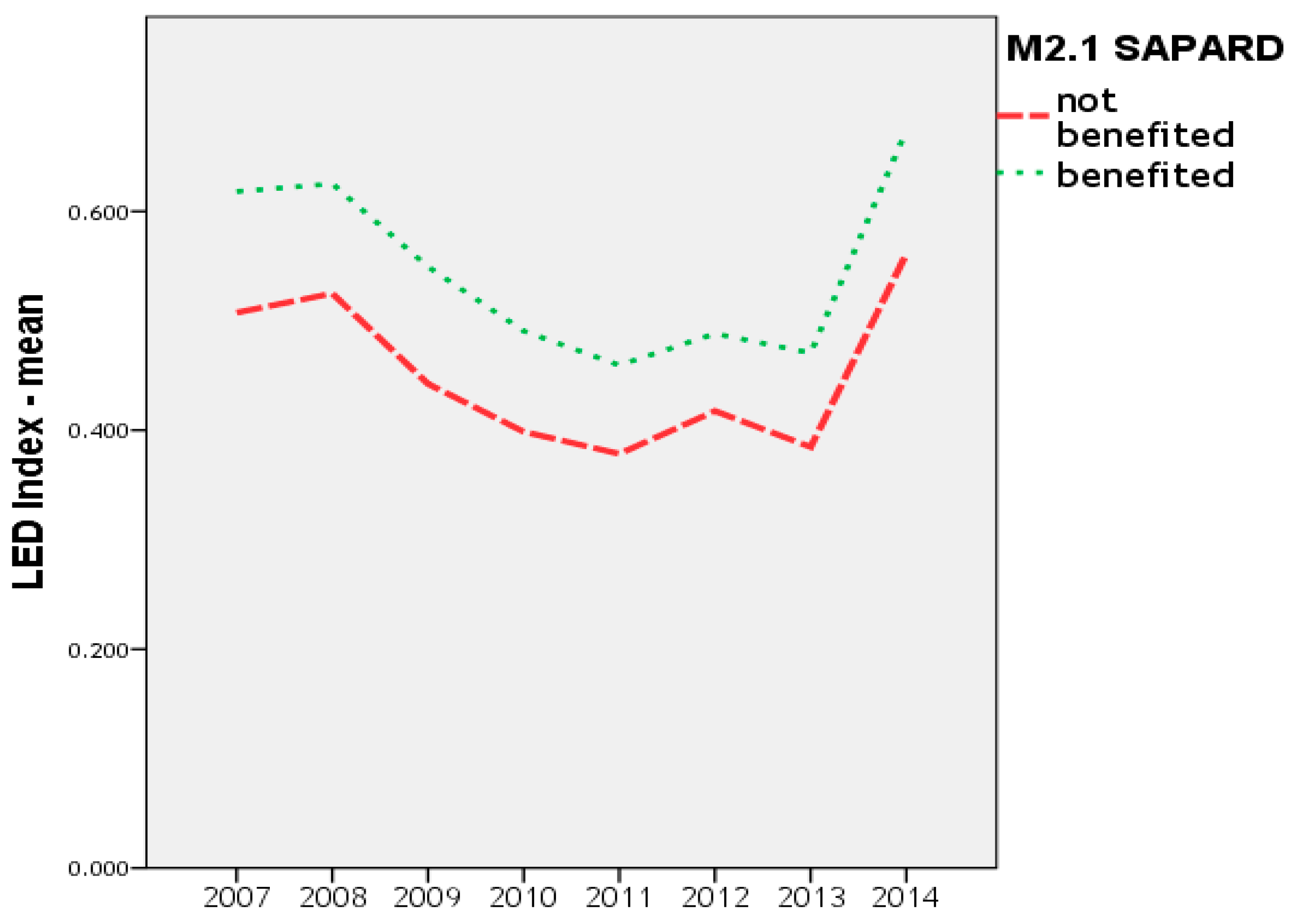
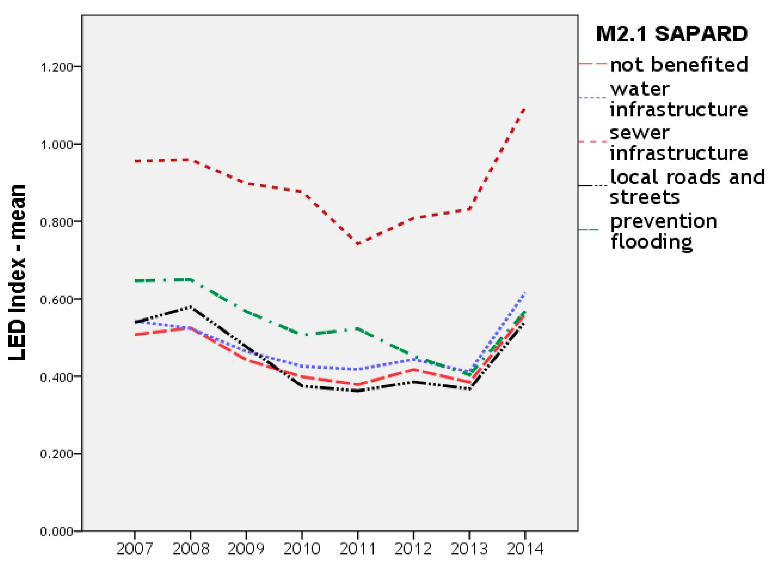
• SAPARD (Special Accession Programme for Agriculture and Rural Development), Measure 2.1—Developing and improving rural infrastructure was a pre-accession non-refundable program from the European Union. Through this program, based on project competitions/calls for applications, communes could introduce or modernize water infrastructure or sewer infrastructure or modernize local roads and streets or prevent flooding—however, only one category of intervention was eligible per commune. A total of 67 communes benefited from these non-refundable programs for infrastructure in the N-W region: 27 projects for water systems, 14 projects for sewer systems, 24 projects for local roads and streets, and two projects for preventing flooding. Although the program started to be implemented in 2002, actual projects started in 2004 and were finalized until 2009: One (1.49%) project was finalized in 2005, 20 (29.85%) projects were finalized in 2006, 17 (25.37%) in 2007, 17 (25.37%) in 2008 and 12 (17.91%) in 2009. The average value of the payments made (average cost) for the projects financed by M 2.1 SAPARD in N-W region was 758,989.37 € per project; by type of investment, the average cost was 670.459.00 € for a water network project, 810,636.44 € for a sewerage project, 857.233,98 € for a project targeting local roads and 413,864.63 € for a project targeting flooding prevention.
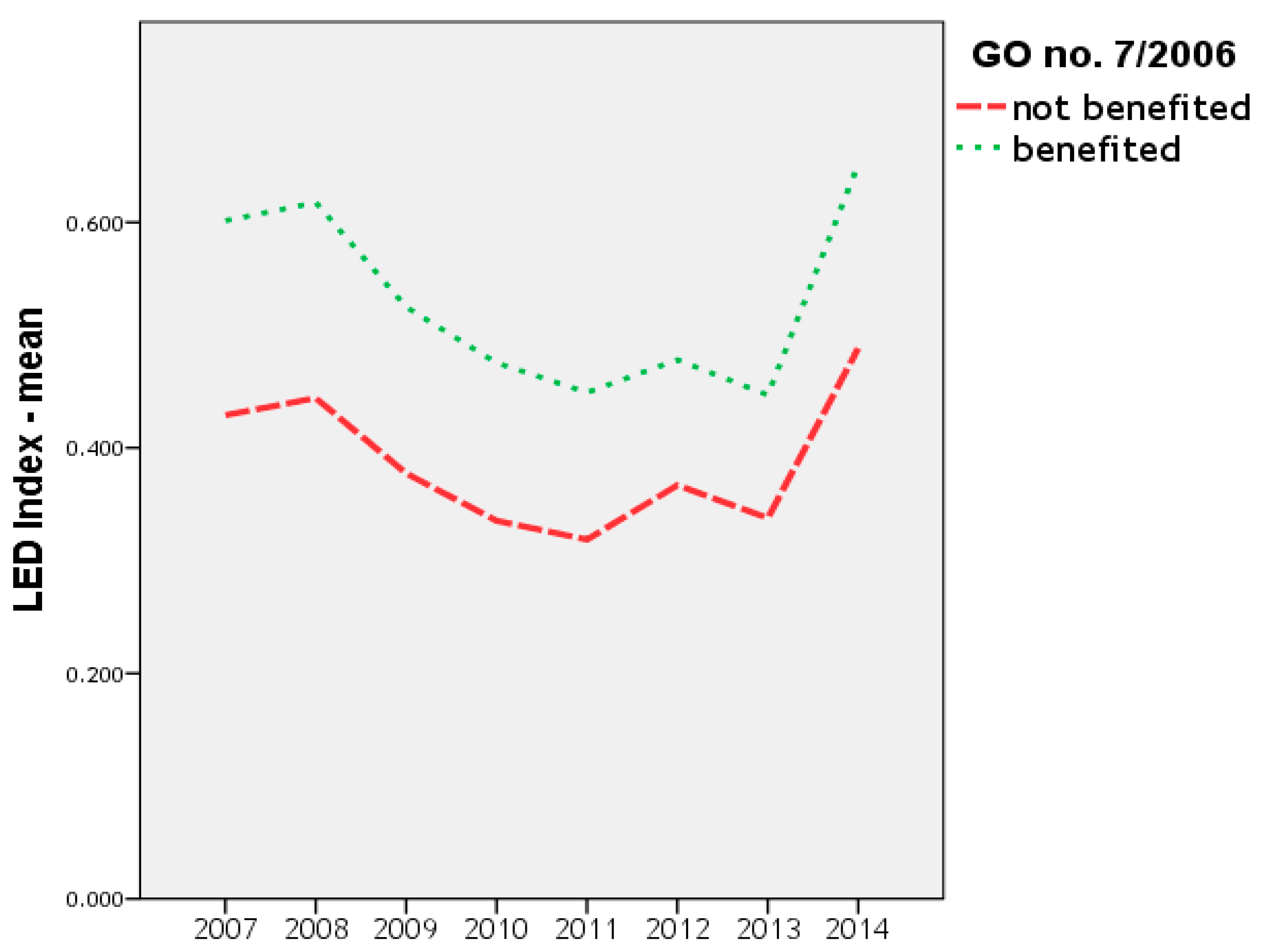
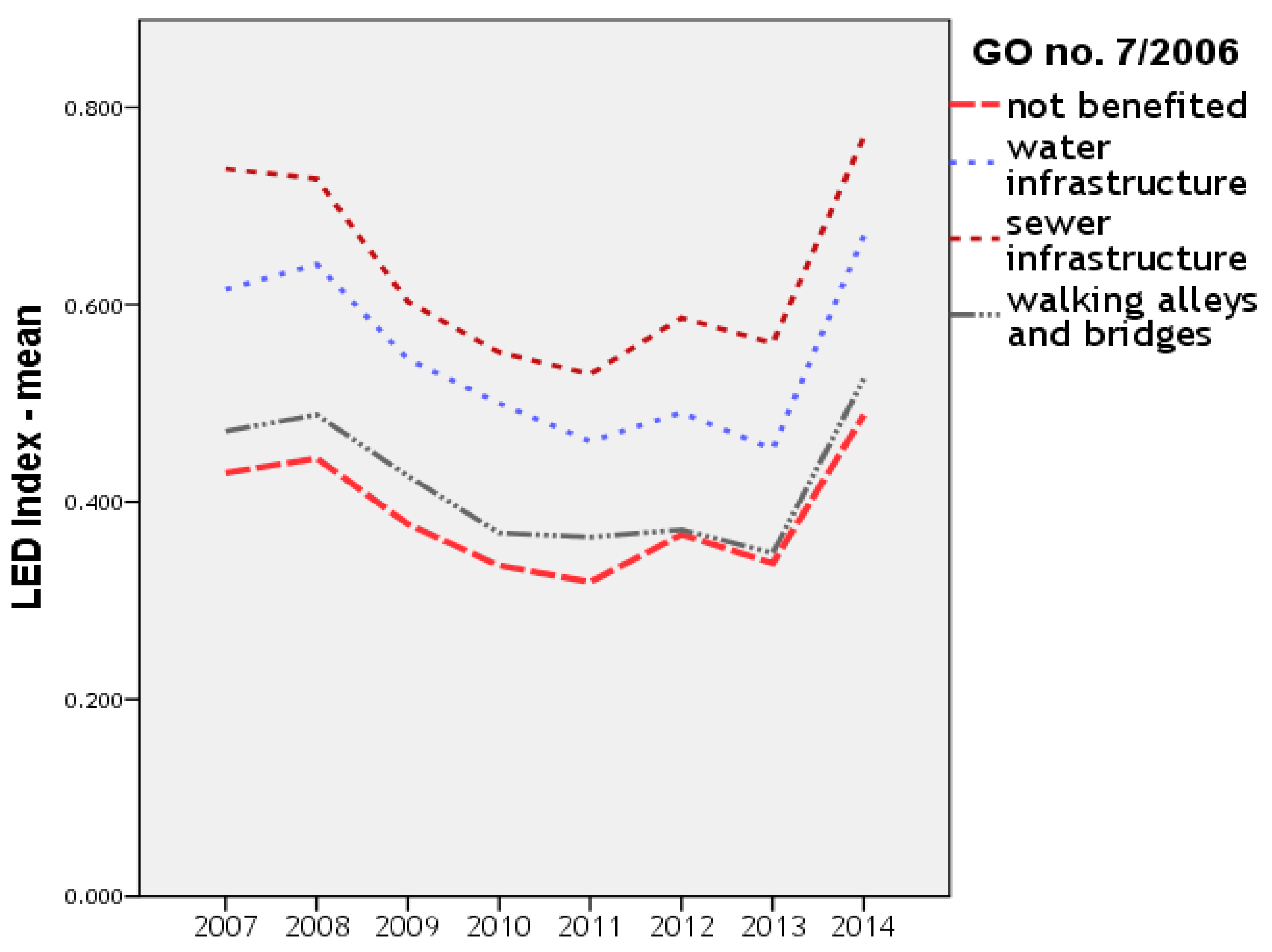
• The Program for Developing Infrastructure and Sport Establishment in the Rural Space (Government Ordinance no. 7/2006) was a state (national) non-refundable program. The perception over the Government Ordinance no. 7/2006 (GO no. 7/2006) was a negative one in the national press, reports of some Non Governmental Organizations and in the Court of Accounts’ reports, often signaling the existence of political clienteles, lack of transparency, lack of monitoring, uncompetitive and unlawful (corrupt) allocation of funds [34]. A total of 225 communes from the N-W region benefited from this program for projects aimed to introduce or modernize water infrastructure (121 communes), sewer infrastructure (45 communes), build/modernize walking alleys and bridges (59 communes). The payments made (average cost) for one project funded by GO no. 7/2006 in the N-W region was approximately 428.934,9 € per project, and by type of investment, the average value of the allocations until 2011 was: 454,098.6 € for a water network project, 569,023.3 € for a sewerage network project and 276,533.3 € for a walking alleys and bridges project. The projects included in this research were implemented between 2007 and 2011. The main research limitation in the case of this program is that in 2011, the stage of those 225 projects is still unclear: We do not know if they have been finalized or not or what their implementation stages are (10% or 50% or 90%).

Our second independent variable (the rank of the commune) refers to the area of influence where a commune is located; communes can be located in the immediate vicinity of a big city or they can be isolated (deep-rural communities). As multiple studies [35,36,37,38,39] have concluded, proximity to a large urban area can exert a positive influence on the surrounding rural communities, while spatial (geographical) isolation from large urban centers can often condemn rural communities. We used the Study for the substantiation of an update of the plan for landscaping the national territory [40] for the rank of the commune as the study establishes the basic principles for organizing the network of localities in Romania, the strategic objectives that will underpin the development and structuring of the network of localities and the criteria on which localities can be hierarchized. Starting from this ranking and mapping, we grouped the N-W communes in six types or categories of functional areas as follows:

• “Territorial groups of Rank I (TG-R I 6),” formed around a large city with a minimum of 100,000 inhabitants (includes a large city and the communes around); the communes located in these territorial clusters will have the Rank 6. The commune situated around the cities of Cluj-Napoca, Oradea and Satu Mare are included in this category;
• “Urban agglomerations of Rank II (UA-R II 5),” with over 200,000 inhabitants and at least one large city of over 100,000 inhabitants (includes large cities, small and medium-sized cities and the surrounding communes); the communes located in these areas will have the Rank 5;
• “Territorial groupings of Rank II (TG-R II 4),” formed around a large/medium city with a minimum of 50,000 inhabitants (includes a medium/large city and the surrounding communes); the communes located in these areas will have the Rank 4;
• “Urban agglomerations of Rank III (UA-R III 3),” with more than 100,000 inhabitants and at least one large city having over 50,000 inhabitants (includes medium and small cities and communes); the communes located in these areas will have the Rank 3;
• “Territorial groupings of Rank III (TG-R III 2),” formed around a medium/small city with a minimum of 20,000 inhabitants (includes medium/small towns and communes); the communes located in these areas will have the Rank 2;
• “Rural Territorial Groups (RTG-R I 1),” consist of one or more villages clustered around an administrative village (commune residence village); they are outside the influencing area of any cities and can be considered “isolated” communities or the most representative communities for the Romanian rural space; the communes located in these territorial clusters will have the Rank 1.

Direct connection to E-Road Network refers to the situation in which a road part of the E-Road (network system for roads in Europe developed by the United Nations Economic Commission for Europe) crosses the territory of a commune, thus linking it with the broader area. Direct connection to the (Romanian) National Roads Network refers to the situation in which a road part of the National Network Roads (excepting the roads included in the E-road network) crosses the territory of a commune. Direct connection to E-Road and National Network Roads are used as explanatory variables because the transport infrastructure can stimulate economic activity and economic growth [11,27,41,42,43,44].

Population size was included as an independent variable as, although multiple studies [45,46,47,48,49,50] assumed that population size influences LED, no consensus has been reached if the influence is positive or negative. Considering the size of the population, the communes were grouped into six categories, as follows: Category 1—up to 1500 inhabitants; Category 2—from 1501 to 3000 inhabitants; Category 3—from 3001 to 4500 inhabitants; Category 4—from 4501 to 6000 inhabitants; Category 5—from 6001 to 7500 inhabitants, and Category 6—more than 7500 inhabitants.

The percentage of university graduates was included as an independent variable based on the findings of [51,52,53,54,55]. This indicator was calculated based on the 2011 Population Census Data, for each commune, as a share of the total population.

Considering the all the aforementioned independent variables, the description of the 398 communes included in our sample is provided in Appendix A. Although our main research interest refers to the impact that non-refundable financing programs for infrastructure (as exogenous factors) have on LED, the other variables were included in the model as control variables.

4. Results and Discussions

In order to reach our research objective, we will initially discuss how the LED index was created using the Principal Component Analysis (PCA) (in Section 4.1.) and then present the evolution of local economic development according to each independent variable (in Section 4.2, as an exploratory analysis) and the results of multiple regression models which try to explain LED based on the aforementioned independent variables (in Section 4.3, as an confirmatory analysis).

4.1. The LED Index. An Exploratory Analysis of Its Influencing Factors

Before exploring the factors which can influence LED, we will briefly present the index we constructed based on the factorial analysis of the 10 variables included in Table 1. Although the construction of the LED index is based on a similar methodology and partially on the same data as Pavel, Moldovan, Neamțu and Hințea [32], we chose to include it in order to offer a more accurate depiction of the dependent variable and the methodology behind its construction. The values from the matrix of the PCA (the first component extracted), the KMO and Bartlett’s Test values, the total variance explained by the first component extracted and the total number of extracted components are included in

Table 3. The main results of the Principal Components Analysis (PCA) (2007–2014).

Indicators/Year	2007	2008	2009	2010	2011	2012	2013	2014
Factor Loadings for the First Component Extracted
Turnover per capita	0.896	0.901	0.836	0.876	0.836	0.886	0.906	0.896
Turnover per employee	0.400	0.320	0.461	0.451	0.424	0.477	0.431	0.376
Average number of employees per 1000 inhabitants	0.888	0.915	0.925	0.921	0.922	0.936	0.953	0.936
Number of employees/elderly (retired) population	0.880	0.903	0.915	0.909	0.911	0.913	0.940	0.927
Income from income tax breakdowns per capita	0.688	0.600	0.689	0.742	0.757	0.839	0.823	0.813
Income from local taxes per capita	0.418	0.524	0.681	0.702	0.545	0.549	0.514	0.604
Active business density	0.857	0.876	0.819	0.756	0.760	0.741	0.714	0.755
Entrepreneurial capacity	0.630	0.712	0.441	0.122	0.192	0.207	0.097	0.595
Social assistance expenses per capita	−0.324	−0.308	−0.191	−0.330	−0.153	−0.105	−0.086	−0.041
Number of dwellings completed during the year per 1000 inhabitants	0.476	0.504	0.515	0.408	0.509	0.484	0.480	0.459
Indicators
KMO	0.787	0.844	0.835	0.832	0.799	0.809	0.794	0.819
Bartlett’s Test for Sphericity	2776.435	2798.656	2537.383	2566.776	2405.117	2665.028	2768.782	3136.446
Total variance explained by the first component extracted (%)	46.366	48.264	47.079	45.510	43.267	45.633	44.973	48.402
Number of components	2	2	2	2	2	2	3	3
N	398	398	398	398	398	398	398	398

The significance of Bartlett’s Test for Sphericity was 0.000 for each year of the analysis. Source: The authors.

.

The KMO (which measures sample adequacy) is well over 0.5 for each year, indicating a very high level of adequacy of the correlation matrix and the fact that the indicators used are appropriate for aggregation using PCA; the significance of Bartlett’s test of Sphericity (which stands at 0.000) recommends continuing the analysis (Table 3). The first factor extracted in each year explains more than 44% of the total variance and the low number of extracted factors (two for six years and three for two years) further confirms that the indicators are appropriate for aggregation.

The values for the first component extracted show that the most relevant indicators used for aggregation are the average number of employees (per 1000 inhabitants), the number of employees/elderly (retired) population (which can be regarded as a social sustainability indicator), turnover (per capita), budgetary revenues from personal/company income tax breakdowns (per capita) and active business density; their weight is closer to 1 than to 0 and they are almost constant for the analyzed period. Entrepreneurial capacity and social assistance expenses (per capita) are the indicators with the lowest weights (loadings) and the most inconstant values during the period; as we expected, social assistance expenses (per capita) are negatively weighted in the first component extracted.

During the following stage of our research, we explored potential connections between the seven independent variables (included in Table 2) and the LED index constructed.

4.2. Exploratory Analysis of the Factors Which Can Influence LED

The mean of the LED index for the communes which benefited (or did not) from M2.1 SAPARD (European Union non-refundable program for basic infrastructure in rural communities) is presented in Figure 1. Figure 1 shows that beneficiaries of M2.1 SAPARD have had (on average) a higher level of LED from the initial moment of the analysis (in 2007, only 31.34% of the projects have been finalized, 1.49% in 2005 and 29.85% in 2006). However, as Janeski and Whitacre [30] revealed, the impact of this kind of project (water and sewer infrastructure) on the local economy is rather on the medium and long term. As such, we posit that the difference in the level of LED between beneficiary and non-beneficiary communes in 2007 is not due to the impact of the investments made in base/core infrastructure, but rather that LED differences already existed in the initial moment (2002), when communes applied/competed for this non-refundable program (M2.1 SAPARD). More developed communes had a higher capacity (including administrative capacity) to complete the documentation (the application form, feasibility study) or to pay consultancy companies to ensure their success in attracting non-refundable funding.

Looking at the evolution of the LED Index between 2007 and 2014, and considering that all the projects have been implemented until 2009, we do not see any significant (positive) change in the evolution of the beneficiaries after the projects were finalized. We can also observe in Figure 1 that the difference of the LED Index (between the two categories) is almost the same in 2007 and in 2014. In 2007 the mean of LED Index for M2.1 SAPARD beneficiaries was 0.618 and for no beneficiaries was 0.507 (21.8% lower), while in 2014 the mean of LED Index for M2.1 SAPARD beneficiaries was 0.674 and for no beneficiaries was 0.561 (20.1% lower). As such, we can argue that non-refundable EU investments (M2.1 SAPARD) in basic/core infrastructure in rural communities (communes) from the N-W region of Romania did not boost their LED (at least on short and medium term). However, when considering the kind of infrastructure developed through M2.1 SAPARD (see Figure 2) we observe that communes who implemented sewer infrastructure projects were the most developed in 2007 and they are in the same position in 2014.

The communes that invested in water infrastructure and local roads and streets have had the same level of LED in 2007 (higher than non-beneficiaries), but while communes that invested in water infrastructure kept the position higher than non-beneficiaries, the communes that invested in local roads and streets have a lower LED than non-beneficiaries after 2010 (see Figure 2). From this perspective, the EU non-refundable investments in local roads and streets do not seem to have any positive impact on LED (projects aiming to prevent flooding are not representative/significant as only two communes implemented these projects).

Similar to the situation of M2.1 SAPARD non-refundable program, the beneficiaries of GO 7/2006 (the national non-refundable program included in the analysis) had (on average/mean) a higher level of LED (see Figure 3) from the beginning of the program implementation (2007). We can assume that the same rationale, as in the case of European funding, applies to national funding: Communes which were more developed initially had a higher capacity to complete the application form (or to seek external help), thus ensuring their success in attracting non-refundable funding.

Although we did not find any information regarding the implementation stage for the 225 projects financed by GO 7/2006, we can observe in Figure 3 that the difference between beneficiaries and non-beneficiaries has decreased from 2007 to 2014. If in 2007 the mean value of the LED Index for beneficiaries was 0.601 and for non-beneficiaries was 0.429 (40.5% lower), in 2014 the mean value of the LED Index for beneficiaries was 0.652 and for non-beneficiaries was 0.488 (33.5% lower). As such, the investments funded by GO 7/2006 do not seem to have any impact on the LED of rural communities from the N-W region; however, a better informed assessment/opinion can only be reached by analyzing the types of projects which were financed, as shown in Figure 4.

When taking into account the type of infrastructure developed through GO 7/2006, the situation is similar with the M2.1 SAPARD program, as communes that implemented sewer infrastructure projects were the most developed in 2007 and they are in the same situation in 2014 (see Figure 4); the situation is similar in the case of water infrastructure investments. In the case of walking alleys and bridges, even if the beneficiaries were more developed in 2007 than non-beneficiaries, the difference decreases considerably by 2014, as shown in Figure 4.

Summarizing, these first findings (from Figure 2 and Figure 4) show that the communes which applied and implemented sewerage system projects (funded from those two non-refundable programs) were more developed in the initial stage compared to those which applied and implemented water systems or local roads or walking alleys and bridges projects. These results could suggest that the communes which applied and implemented sewerage systems were more developed than the communes that applied and implemented other types of local infrastructure projects because they already had a water system and also because the local roads, walking alley and bridges were not considered to be their biggest issue/needs at that stage. Going further with this assumption, we might argue that the higher level of LED is also due to the fact that they had previously introduced water systems, and this helped them develop earlier.

Figure 5 presents the evolution of the LED index according to the rank of the commune. If we exclude communes with the Rank 5, 3 and 2 (due to the low number of cases, thus not being statistically representative) we can observe that communes situated near the largest city in the region are much more developed, while communes situated outside the area of influence of any city are the least developed. Comparing Rank 6 communes (those located near the biggest cities in the region) with Rank 1 communes (those located outside the influencing area of any cities) we can observe that in 2007 the mean value of the LED Index for Rank 1 is 0.417, while for Rank 6 is 1.014 (2.430 bigger). In 2014, the mean value of the LED index for Rank 1 communes is 0.485, while for Rank 6 communes is 1.014 (2.260 bigger). Although the difference between 2007 and 2014 is decreasing in the case of the two ranks, we can also observe that undeveloped communes (rank 1) were less influenced by the 2007/2008 economic-financial crisis as these communes had very little to lose (from an economic point of view) due to their underdevelopment.

The LED index difference between communes with a direct connection to the E-Road Network and those without (Figure 6) is higher during the entire period and decreases only marginally until 2014: In 2007, communes with a direct connection have a mean value for the LED index of 0.774, while for communes without a direct connection the mean LED value is 0.446 (1.734 lower). A similar connection between transport infrastructure and economic development was also made by Gherghina, Onofrei, Vintilă and Armeanu [56] at the EU-28 level, observing that ‘road, inland waterways, maritime, and air transport infrastructure positively influence gross domestic product’ (p. 1) and that investments in public infrastructure ‘exhibit a positive impact on economic growth for every type of transport, except inland waterways’ (p. 1). Similar connections between transport infrastructure and sustainable development were made by Wang, Xue, Zhao and Wang, [57], via a meta-analysis of 2543 articles published from 2000 to 2017.

In 2014, the mean value of the LED Index for communes directly connected to the E-Road Network is 0.835 and for communes without a direct connection the mean value is 0.498 (1.675 lower); as such, the existence of a direct connection to the E-Road Network seems to be an important factor for LED, but the situation differs in the case of the National Roads Network, as shown in Figure 7.

As Figure 7 shows, some differences existed in 2007 between communes with a direct connection to the National Roads Network and those without, but this LED gap is smaller than in the case of the E-Road Network; furthermore, the difference has decreased by 2014. If in 2007, the ratio between the mean value of the LED index in the case of communes with a direct connection and those without a direct connection is 1.262, in 2014 the ratio decreases slightly to 1.142.

Figure 8 indicates the existence of a directly proportional relationship between the population size of the communes and LED; in brief, the bigger the communes are the bigger the mean value of the LED Index is. Furthermore, in the case of the biggest communes (those with over 7500 inhabitants) the difference seems to be exponential and these are located near/at the border of the biggest cities in the region (Rank 6). The difference between the largest and smallest communes is decreasing from 2007 to 2014 as the smallest/lowest developed communes in the region (with under 1500 inhabitants) do not appear to be affected by the economic crises started in 2007/2008, while the biggest (more developed) communes seem to be the most affected. If in 2007 the ratio between the mean value of the LED Index for the biggest communes and the mean value of the LED Index for the smallest communes is 4.573, the ratio decreases to 2.422 (almost half) in 2014.

One of the interesting findings of the exploratory analysis consists in the fact that investments in the water network and especially those in the sewerage network seem to influence the economic development of rural communities more than investments in local roads, bridges and walking alleys. Although at first glance these results may seem surprising, they can be justified from an economic point of view as water and sewage networks are essential for the establishment, operation and development of economic units, especially production units which are subject to environmental protection rules and regulations. The production process is impossible without access to a water network and the possibility of dealing with the resulting waste water. A production unit (such as a dairy/cheese factory, fishery, fruit/vegetable packing and so on) can be opened in a community where water and sewerage networks exist, even if local roads that facilitate access to the production unit are not asphalted, but are just cobbled and maintained; however, the production unit will not be able to operate in a commune where there is no running water and a sewerage network, even if the local roads are paved, the commune is located near a big city, the population is young and qualified, and so on.

4.3. Confirmatory Analysis: Assessing the Main Determinants of LED

In order to confirm the influence of the independent variables (included in Table 2) on LED (as previously observed in Figure 1, Figure 2, Figure 3, Figure 4, Figure 5, Figure 6, Figure 7 and Figure 8) we continued with four linear regression models. In the first two models (

Table 4. Regression models summary and determinants for the level of LED.

Independent Variables		Model A					Model B
		B	Std. Error	Beta	t	Sig	B	Std. Error	Beta	t	Sig
Rank		0.070	0.010	0.278	7.323	0.000	0.097	0.011	0.385	8.539	0.000
Direct connection to the E-Road Network		0.098	0.040	0.094	2.453	0.015	0.229	0.047	0.221	4.910	0.000
Direct connection to the National Roads Network		0.033	0.039	0.031	0.841	0.401	0.099	0.047	0.092	2.096	0.037
Population size		0.040	0.015	0.102	2.654	0.008
Percentage of university graduates		9.359	0.741	0.495	12.624	0.000
Model summary	R Square	0.486					0.240
	R	0.697					0.490
	F	74.254					41.496
	Sig.	0.000					0.000

Source: Compiled by the authors.

), the dependent variable (the level of LED) was computed as the arithmetic mean of the LED index values for the period included in the analysis (from 2007 to 2014). Table 4 explains the relationship between the level of LED and its main determining factors, excluding the two non-refundable investments programs (SAPARD and GO 7/2006) which can only influence the level of LED in the long run (as more time would be necessary for these investments to manifest their effects). Since investments projects were still being implemented in the analyzed period, we cannot assume or expect that these two programs had, up to this point, any influence/impact on the LED level (i.e., the level of LED precedes, from a temporal point of view, the two programs)—the same argument regarding the long run effect of investments was also presented by Pavel, Moldovan, Neamțu and Hințea [32].

Model A measures the causal relationship between the five proposed factors which can influence the level of LED and the index we constructed, while in Model B, due to potential endogeneity regarding the percentage of university graduates, the population size and the level of LED (and also considering the lack of some instrumental variables) we excluded these two independent variables and measured the causal relationship between the other three remaining independent factors and the level of LED (see Table 4).

The regression shows which independent variables influence the level of economic development as approximated by the LED index we previously constructed. In the case of Model A, R² indicates that the explanatory power of the model is medium to strong, as the independent variables explain 49% of the variation of the arithmetic mean of the LED index. The main statistically significant predictors of LED are the percentage of university graduates (0.495***) and the rank of the commune (0.278***). Population size and direct connection to the E-Road Network are weak predictors for the level of LED in Model A, while direct connection to the National Roads Network is not a predictor for LED in rural communities from the North-West Region of Romania (see Table 4).

In the case of Model B from Table 4, the explanatory power is smaller (0.240), but the model is statistically significant (0.000). Model B (which is less susceptible to endogeneity concerns) reconfirms that the rank of the commune is the main statistically significant predictor for the level of LED, followed by direct connection to the E-Road Network. Reducing the potential threat of endogeneity by eliminating the percentage of university graduates and the population size, Model B also proves the robustness of the variable rank of the commune, confirming the theory stating that location or proximity to an urban area (big urban area) has a significant influence on LED [11,35,36,37,38,39]. Furthermore, we ran regression Model B only for Rank 1 communes (referring to 294 communes—the “isolated” communities or the most representative communities for the Romanian deep-rural space); when excluding the rank from the regression model the explanatory power decreases considerably (R² = 0.060, Sig. = 0.000). These results confirm that for the most isolated rural communities, an important predictor for LED is the direct connection to the E-Road Network (Beta = 0.203***) and, in this case (isolated rural communities), direct connection to the National Roads Network. In conclusion, the regression model confirms that direct connections to the E-Road Network and the National Roads Network are significant predictors for the level of LED in the case of isolated communities.

The next two models (included in

Table 5. Regression model summary and determinants for spurring LED.

Independent Variables		Model C					Model D
		B	Std. Error	Beta	t	Sig	B	Std. Error	Beta	t	Sig
Rank		0.001	0.004	0.010	0.197	0.844	0.000	0.003	−0.007	−0.141	0.888
Direct connection to the E-Road Network		0.034	0.015	0.125	2.332	0.020	0.025	0.014	0.092	1.754	0.080
Direct connection to the National Roads Network		0.009	0.015	0.030	0.594	0.553	0.003	0.015	0.011	.213	.831
Population size		−0.015	0.006	−0.138	−2.537	0.012
Percentage of university graduates		−0.172	0.280	−0.034	−0.614	0.540
M2.1, SAPARD	water infrastructure	0.025	0.023	0.055	1.075	0.283	0.017	0.023	0.038	0.744	0.457
	sewer infrastructure	0.006	0.018	0.016	0.318	0.751	−0.005	0.018	−0.014	−0.284	0.776
	local roads and streets	0.007	0.008	0.044	0.858	0.391	0.006	0.008	0.034	0.677	0.499
GO 7/2006	water infrastructure	0.000	0.014	0.002	0.034	0.973	−0.003	0.014	−0.013	−0.236	0.814
	sewer infrastructure	0.000	0.020	−0.001	−0.022	0.982	−0.008	0.020	−0.020	−0.379	0.705
	walking alleys and bridges	−0.025	0.018	−0.076	−1.410	0.159	−0.025	0.018	−0.076	−1.403	0.161
Model summary	R Square	0.034					0.016
	R	0.185					0.125
	F	1.250					0.682
	Sig.	0.252					0.726

Source: The authors.

) measure the degree in which the aforementioned factors (independents variables) spur/accelerate LED. In this case the dependent variable was the average growth rate (computed according to Equation (1)). The average growth rate based on the LED Index was calculated according to the following autoregressive formula:

$${\mathrm{LED}}_{AGR}=\frac{{{\displaystyle \sum }}_{t=2}^T{y}_t\ast y_{t-1}}{{{\displaystyle \sum }}_{t=2}^T{(y_{t-1})}^2},$$

(1)

where LED_AGR is the average growth rate of LED from 2007 to 2014 and y_t represents the level/value at a given moment in time of LED. We choose this autoregressive model to measure the average growth/decrease rate instead of others because it captures more accurately and reliably each change of value from one year to another for all-time series.

In the case of Table 5, Model C measures the causal relationship between the proposed factors which can spur local economic development and average growth of the index we constructed. In the case of Model D, we excluded the percentage of university graduates and the size of the population due to potential endogeneity issues in order to obtain more reliable results.

In the case of Table 5, the regression models (in which the dependent variable is the average growth rate) should offer more insights into the factors which can actually stimulate/spur LED. The explanatory power of Model C is rather reduced, not statistically significant (with R² = 0.034 and Sig. = 0.252), and none of the non-refundable investments made in basic infrastructure were conducive to an increase in LED in the analyzed period. Model C identified only two weak predictors for spurring/accelerating LED in the communes, namely direct connection to the E-Road Network (0.125*) and population size (−0.138*). The relationship between the population size and the average growth rate of the LED Index is negative, meaning that population growth was actually harmful to local economic development. In Model D we excluded from the list of independent variables the percentage of university graduates and the population size (due to potential endogeneity issues) and, as expected, the explanatory power is lower than in Model C and not statistically significant. However, we consider that in the case of Model C, endogeneity is not an issue/threat for our results because the dependent variable—average growth rate—measures the evolution of LED in a short period of time (8 years); thus, it cannot be argued that due to a good development of the local economy the percentage of university graduates increased significantly in such a short time span.

We conducted another regression in which we used as independent variables in the model only the different types of nonrefundable investments made in local core infrastructure and as the dependent variable the average growth of LED (measured as we showed earlier in Equation (1)). As expected, the explanatory power of the model is almost 0 but the results corroborate that, at least in the short run, exogenous factors such as non-refundable funds for local basic infrastructure do not spur LED in rural communities.

5. Conclusions

The current research allowed us to identify the main factors which influence the level of LED in 398 communes from the North-West development region of Romania during the 2007–2014 period. Using a linear regression model, we also observed the main statistically significant predictors for the level of LED, in order of their importance: The percentage of university graduates, location in the influence area of urban communities and the existence of a direct connection to the E-Road Network. If we eliminate the percentage of university graduates and the population size from the regression model (in order to reduce potential endogeneity concerns) the results confirm that location (or proximity to a big urban area) and direct connection to the E-Road Network remain two of the most important determinant factors for the level of LED. On the other hand, our study shows that the rank of the commune (used as a proxy for location), the percentage of university graduates and direct connection to the National Roads Network are not determinant factors for spurring LED in a short period (8 years). Only direct connection to the E-Road Network is a weak predictor for spurring LED while population size of rural communities seems to be a negative predictor for accelerating LED.

Our study shows that, in the short run, exogenous factors such as non-refundable investments in local (core) infrastructure (including water infrastructure, sewer infrastructure, roads and walking alleys and bridges) do not have any statistically significant influence on accelerating LED. Our results are similar to those obtained by Pavel, Moldovan, Neamțu and Hințea [32] in their analysis of the influence of non-refundable investments (for the construction and modernization of basic infrastructure, development of basic community infrastructure for recreation, education, health care, etc., and preservation of cultural built heritage from rural areas) on LED, as the impact of these projects seems to be only marginal. As the aforementioned authors [32] explained, the conclusion that impact is marginal refers only to the short run and only regarding local economic development. However, we do not want to induce or promote the idea that investments in core local infrastructure are useless; even in the short run there can be certain direct and indirect benefits for the people living in rural communities, but these benefits are more likely linked with the quality of life. Once public utilities (water and sewage) are functional they lead to a better life, increasing the level of sanitation, reducing the level of water and soil pollution, reducing the level of illness, etc. It is also obvious that local roads, walking alleys and bridges facilitate access to public services (kindergarten, school, medical office, local authorities) and workplaces.

Looking at both types of non-refundable programs (M2.1 SAPARD and GO no. 7/2006) we can posit that communes which were more developed initially (in 2007) had a higher capacity (including administrative capacity) to complete the application form (or to seek consultancy) and this ensured their success in attracting non-refundable funding. However, policy makers seem to have also observed this “limitation,” as the successor of M2.1 SAPARD in Romania (namely Measure 322 of the National Plan for Rural Development) facilitated, through the evaluation criteria, access to non-refundable financing for the less-developed (disadvantaged) rural communities [32].

Another important finding is that no matter the source (EU or national) of non-refundable investments in local core infrastructure, the most developed communes are those that invested in the sewerage infrastructure, followed by those who invested in the water infrastructure and then by those who have invested in local roads bridges and walking alleys. The study also reveals that these communes, exactly in the aforementioned order, were already more developed in the initial phase, respectively before the infrastructure investments were made and the development difference was maintained throughout the analyzed period. It seems that only the most developed communes had the administrative capacity to carry out projects and access non-refundable programs, but these investments did not spur LED. Moreover, the study shows that the most wanted/desirable investments by local authorities from the Romanian rural area (namely those in local roads) have no impact on LED and the difference of LED between the commune that invested (through non-refundable program) in local roads and those communes that did not invest decreased over time. Thus, we would recommend extra-diligence when deciding how to invest limited public financial resources [58], following a strategic approach [59], especially in the context of financial crises [60] or underperforming local revenue mobilization [61]; we also need to take into account the relationship between good/quality governance and growth [62,63].

We also need to mention the main limitations of our research. The first regards the impossibility of composing the LED index from the initial stage of the SAPARD program (2002) due to the fact that many of the indicators used for aggregation were not available before 2006. Methodologically, it would be ideal to create the LED index starting with 2002 and to use the difference-in-differences method in order to evaluate the impact that non-refundable investments in core infrastructure have on the LED of rural communities. Another research limitation consists of the fact that the projects funded from the two non-refundable programs were not implemented in the same time and have not been finalized in the same year. Further limitations of the research refer to the lack of data regarding the stage of the projects funded from GO no. 7/2006 (if they were finished or not in 2011) and the weak explanatory power (lack of statistical significance) of Models C and D (however, we strongly believe that these models can be improved in future research and thus has the potential to lead to more robust results). Another limitation refers to potential endogeneity issues: Unfortunately, we did not find any relevant instrumental variables in order to eliminate it, but we reduced it by excluding the main variables supposed to contribute to the endogeneity of the regression models. Since the research is focused on both a European financial instrument (the M2.1 SAPARD) and a national Romanian program (Government Ordinance no. 7/2006) the methodological approach and the analyses are not extensible worldwide, but they are relevant for the EU space (including pre-accession countries) where EU and national programs coexist and, in more general terms, for other contexts where national and international (or foreign aid) programs are implemented simultaneously.

The research can be extended to the entire rural area of Romania in order to evaluate the LED impact of these and other non-refundable programs in local core infrastructure or that of other endogenous or exogenous factors. It would be also very interesting, as potential future research, to evaluate the impact of non-refundable programs in local core infrastructure in the long run (at least 10 years after implementation). Usage of the difference-in-differences method and the propensity scores method can significantly enhance the quality and reliability of future studies regarding the impact of non-refundable programs in local core infrastructure on LED. Furthermore, although the current data did not allow, future research on sustainable local development can and should also take into account inter-community cooperation [64,65], coordination [66] and even community resilience [67,68] or sustainable competitiveness [69] between rural communities (although these concepts might prove to be more problematic to quantify and measure adequately). Other future research potential lies in changing the focus from exogenous factors (such as those analyzed in this article) to endogenous ones, thus shifting the approach from top-down local economic development to the more complex and nuanced bottom-up Community Lead Local Development (CLLD) model [70,71,72].

References

- Academy of Economic Studies. Studiu Privind Potențialul-Socio-Economic de Dezvoltare al Zonelor Rurale [Study Regarding the Socio-Economic Potential of Rural Areas]; Study Conducted for the Ministry of Agriculture and Rural Development from Romania; Academy of Economic Studies: Bucharest, Romania, 2014; Available online: http://www.madr.ro/docs/dezvoltare-rurala/programare-2014-2020/studiu-potential-socio-economic-de-dezvoltare-zone-rurale-ver-10.04.2015.pdf (accessed on 2 June 2018).
- Ecosfera V.I.C. S.r.l/Agriculture Capital & Engineering. Raportul Final de Evaluare Ex-Post SAPARD România—Evaluarea Ex-Post Privind Implementarea Programului SAPARD în România în Perioada 2000–2008 [SAPARD Final Ex-Post Evaluation Report Romania—Ex-Post Evaluation of SAPARD Program Implementation in Romania in 2000–2008]; Agriculture Capital & Engineering: Bucharest, Romania, 2011; Available online: http://old.madr.ro/pages/dezvoltare_rurala/sapard/Raport-Final-Evaluare-ex-post-SAPARD.pdf (accessed on 2 June 2018).
- Swinburn, G.; Goga, S.; Murphy, F. Local Economic Development: A Primer Developing and Implementing Local Economic Development Strategies and Action Plans; World Bank: Washington, DC, USA, 2006; Available online: http://documents.worldbank.org/curated/en/763491468313739403/pdf/337690REVISED0ENGLISH0led1primer.pdf (accessed on 2 June 2018).
- Blakely, E.J.; Bradshaw, T.K. Planning Local Economic Development: Theory and Practice; SAGE Publications: Thousand Oaks, CA, USA, 2002. [Google Scholar]
- Blakely, E.J.; Green, L.N. Planning Local Economic Development: Theory and Practice; SAGE Publications: Thousand Oaks, CA, USA, 2009. [Google Scholar]
- Palavicini-Corona, E.I. Local Economic Development in Mexico: The Contribution of the Bottom-Up Approach. Ph.D. Thesis, London School of Economics and Political Science, London, UK, 2012. Available online: http://etheses.lse.ac.uk/507/ (accessed on 2 June 2018).
- Stöhr, W.; Taylor, F. (Eds.) Development from Above or Below? The Dialectics of Regional Planning in Developing Countries; John Wiley and Sons: Chichester, UK, 1981; ISBN 9780471278238. [Google Scholar]
- Simms, A.; Freshwater, D.; Ward, J. The rural economic capacity index (RECI): A benchmarking tool to support community-based economic development. Econ. Dev. Q. 2014, 28, 351–363. [Google Scholar] [CrossRef]
- Wong, C. Developing indicators to inform local economic development in England. Urban Stud. 2002, 39, 1833–1863. [Google Scholar] [CrossRef]
- Helmsing, B.A.J.H. Partnerships, Meso-Institutions and Learning. New Local and Regional Economic Development Initiatives in Latin America; Institute of Social Studies: The Hague, The Netherlands, 2011. [Google Scholar]
- Rives, J.M.; Heaney, M.T. Infrastructure and local economic development. J. Reg. Anal. Policy 1995, 25, 58–73. [Google Scholar]
- Michalek, J.; Zarnekow, N. Application of the rural development index to analysis of rural regions in Poland and Slovakia. Soc. Indic. Res. 2011, 105, 1–37. [Google Scholar] [CrossRef]
- Bartik, T.J. Evaluating the Impacts of Local Economic Development Policies on Local Economic Outcomes: What Has Been Done and What Is Doable? Upjohn Institute Working Paper No. 03-89; W.E. Upjohn Institute for Employment Research: Kalamazoo, MI, USA, 2002; Available online: https://doi.org/10.17848/wp03-89 (accessed on 2 June 2018).
- Bryden, J. Rural Development Indicators and Diversity in the European Union; University of Aberdeen and Rural Policy Research Institute: Aberdeen, UK, 2003; Available online: https://www.researchgate.net/profile/John_Bryden3/publication/228865950_Rural_Development_Indicators_and_Diversity_in_the_European_Union/links/0046352f9d1cef2cb8000000/Rural-Development-Indicators-and-Diversity-in-the-European-Union.pdf (accessed on 2 June 2018).
- European Commission. Politica Agricolă Comună (PAC) și Agricultura în Europa—Întrebări și Răspunsuri [Agriculture Common Policy and the Agriculture in Europe—Questions and Answers]; European Commission: Brussels, Belgium, 2013. Available online: http://europa.eu/rapid/press-release_MEMO-13-631_ro.doc (accessed on 2 June 2018).
- Gertler, P.J.; Martinez, S.; Premand, P.; Rawlings, L.B.; Vermeersch, C.M.J. Impact Evaluation in Practice; World Bank: Washington, DC, USA, 2016. [Google Scholar]
- Sandu, D.; Voineagu, V.; Panduru, F. Dezvoltarea Comunelor din România [Development of the Communes in Romania]; National Institute for Statistics and University of Bucharest, Faculty of Sociology and Social Work: Bucharest, Romania, 2009. [Google Scholar]
- Ionescu-Heroiu, M.; Burduja, S.I.; Sandu, D.; Cojocaru, S.; Blankespoor, B.; Iorga, E.; Moretti, E.; Moldovan, C.; Man, T.; Rus, R.; et al. Orașe Competitive, Remodelarea Geografiei Economice a ROMÂNIEI [Competitive Cities: Reshaping the Economic Geography of ROMANIA]; Romania Regional Development Program; World Bank Group: Washington DC, USA, 2013; Available online: http://www.fonduri-ue.ro/images/files/studii-analize/43814/Orase_competitive_-_raport_final.pdf (accessed on 2 June 2018).
- Matei, L.; Anghelescu, S. Fundamentarea keynesiană a politicilor de marketing în dezvoltarea locală [A keynesian substantiation of marketing policies in local development]. Economie Teoretică și Aplicată 2010, XVII, 29–46. [Google Scholar]
- Roberts, P.; Shyam, K.C.; Rastogi, C. Rural Access Index: A Key Development Indicator; World Bank: Washington, DC, USA, 2006. [Google Scholar]
- Li, Y.; Long, H.; Liu, Y. Spatio-temporal pattern of China’s rural development: A rurality index perspective. J. Rural Stud. 2015, 38, 12–26. [Google Scholar] [CrossRef]
- Aschauer, D.A. Is Public Expenditure Productive? J. Monet. Econ. 1989, 23, 177–200. [Google Scholar] [CrossRef]
- Duffy-Deno, K.T.; Eberts, R.W. Public infrastructure and regional economic development: A simultaneous equations approach. J. Urban Econ. 1991, 30, 329–343. [Google Scholar] [CrossRef]
- Easterly, W.; Rebelo, S. Fiscal Policy and Economic Growth: An Empirical Investigation; Working Paper No. 4499; National Bureau of Economic Research: Cambridge, MA, USA, 1993. [Google Scholar]
- World Bank. Infrastructure for Development; World Development Report 1994; Oxford University Press: New York, NY, USA, 1994. [Google Scholar]
- Calderón, C.; Easterly, W.; Servén, L. Infrastructure Compression and Public Sector Solvency in Latin America; Working Papers No. 270; Central Bank of Chile: Santiago, Chile, 2002. [Google Scholar]
- Scandizzo, S.; Sanguinetti, P. Infrastructure in Latin America: Achieving High Impact Management; Latin America Emerging Markets Forum: Bogotá, Colombia, 2009. [Google Scholar]
- Mizutani, F.; Tanaka, T. Productivity effects and determinants of public infrastructure investment. Ann. Reg. Sci. 2010, 44, 493–521. [Google Scholar] [CrossRef]
- Hashimzade, N.; Myles, G.D. Growth and public infrastructure. Macroecon. Dyn. 2010, 14, 258–274. [Google Scholar] [CrossRef]
- Janeski, I.; Whitacre, B.E. Long-term economic impacts of USDA water and sewer infrastructure investments in Oklahoma. J. Agric. Appl. Econ. 2014, 46, 21–39. [Google Scholar] [CrossRef]
- Thadaboina, V. ICT and rural development: A study of Warana wired village project in India. Trans. Stud. Rev. 2009, 16, 560–570. [Google Scholar] [CrossRef]
- Pavel, A.; Moldovan, B.; Neamțu, B.; Hințea, C. Are Investments in basic infrastructure the magic wand to boost the local economy of rural communities from Romania? Sustainability 2018, 10, 3384. [Google Scholar] [CrossRef]
- Prieto-Lara, E.; Ocaña-Riola, R. Updating rurality index for small areas in Spain. Soc. Indic. Res. 2010, 95, 267–280. [Google Scholar] [CrossRef]
- Expert Forum. Clientelismul Politic în Alocarea de Fonduri Către Primării (cu Hartă Interactivă), în Sifonarea de Resurse din Companii Publice [Political Clienteles in Allocating Funds to Mayoralties (with Interactive Map), in the Siphoning of Resources from Public Companies]; Expert Forum: București, Romania, 2013; Available online: https://expertforum.ro/extra/harta-bugetelor/EFOR-rap-anual-2013.pdf (accessed on 2 June 2018).
- Berdegué, J.A.; Carriazo, F.; Jara, B.; Modrego, F.; Soloaga, I. Cities, territories, and inclusive growth: Unravelling urban–rural linkages in Chile, Colombia, and Mexico. World Dev. 2015, 73, 56–71. [Google Scholar] [CrossRef]
- Ahrend, R.; Schumann, A. Does Regional Economic Growth Depend on Proximity to Urban Centres? OECD Regional Development Working Papers No. 2014/07; OECD Publishing: Paris, France, 2014; Available online: https://www.oecd-ilibrary.org/docserver/5jz0t7fxh7wc-en.pdf?expires=1524930602&id=id&accname=guest&checksum=EC28CCB0A894DB616F6777F71B0265D0 (accessed on 2 June 2018).
- Duvivier, C. Does urban proximity enhance technical efficiency? Evidence from Chinese agriculture. J. Reg. Sci. 2013, 53, 923–943. [Google Scholar] [CrossRef]
- Mayer, H.; Habersetzer, A.; Meili, R. Rural–urban linkages and sustainable regional development: The role of entrepreneurs in linking peripheries and centers. Sustainability 2016, 8, 745. [Google Scholar] [CrossRef]
- Cabus, P.; Vanhaverbeke, W. The economics of rural areas in the proximity of urban networks: Evidence from Flanders. J. Econ. Soc. Geogr. 2003, 94, 230–245. [Google Scholar] [CrossRef]
- Ion Mincu University of Architecture and Urbanism (n.d.). Studiu de Fundamentare în Vederea Actualizării PATN—Secțiunea Rețeaua de Localități [Study for the Substantiation of an Update of the Plan for Landscaping the National Territory]. Available online: http://www.mdrap.ro/userfiles/PATN_etapaIII.pdf (accessed on 2 June 2018).
- Jacoby, H.G. Access to markets and the benefits of rural roads. Econ. J. 2000, 110, 713–737. [Google Scholar] [CrossRef]
- Estache, A.; Manacorda, M.; Valletti, T.; Galetovic, A.; Mueller, B. Telecommunications reforms, access regulation, and internet adoption in Latin America. Economia 2002, 2, 153–217. [Google Scholar]
- De Ferranti, D.; Perry, G.E.; Ferreira, F.H.G.; Walton, M. Inequality in Latin America and Caribbean: Breaking with History? The World Bank: Washington, DC, USA, 2004. [Google Scholar]
- Egger, H.; Falkinger, J. The role of public Infrastructure and subsidies for firm location and international outsourcing. Eur. Econ. Rev. 2006, 50, 1996–2015. [Google Scholar] [CrossRef]
- Kim, E.; Hewings, G.; Nam, K.-M. Optimal urban population size: National vs local economic efficiency. Urban Stud. 2013, 51, 428–445. [Google Scholar] [CrossRef]
- Furuoka, F. Population growth and economic development: Empirical evidence from the Philippines. Philipp. J. Dev. 2010, XXXVII, 81–93. [Google Scholar]
- Headey, D.D.; Hodge, A. The effect of population growth on economic growth: A meta-regression analysis of the macroeconomic literature. Popul. Dev. Rev. 2009, 35, 221–248. [Google Scholar] [CrossRef]
- Yegorov, Y.A. Socio-economic influences of population density. Chin. Bus. Rev. 2009, 8, 1–47. [Google Scholar]
- Cincotta, R.P.; Engelman, R. Economics and Rapid Change: The Influence of Population Growth; Population Action International Occasional Paper; Population Action International: Washington, DC, USA, 1997; Available online: https://pai.org/wp-content/uploads/2012/01/Economics_and_Rapid_Change_PDF.pdf (accessed on 2 June 2018).
- Easterlin, R.A. Effects of population growth on the economic development of developing countries. Ann. Am. Acad. Polit. Soc. Sci. 1967, 369, 98–108. [Google Scholar] [CrossRef]
- Pinheiro, R.; Pillay, P. Higher education and economic development in the OECD: Policy lessons for other countries and regions. J. High. Educ. Policy Manag. 2016, 38, 150–166. [Google Scholar] [CrossRef]
- Barra, C.; Zotti, R. Investigating the human capital development—Growth nexus: Does the efficiency of universities matter? Int. Reg. Sci. Rev. 2016, 40, 638–678. [Google Scholar] [CrossRef]
- Lazzeretti, L.; Tavoletti, E. Higher education excellence and local economic development: The case of the entrepreneurial university of Twente. Eur. Plan. Stud. 2007, 13, 475–493. [Google Scholar] [CrossRef]
- Kruss, G.; McGrath, S.; Petersen, I.; Gastrow, M. Higher education and economic development: The importance of building technological capabilities. Int. J. Educ. Dev. 2015, 43, 22–31. [Google Scholar] [CrossRef]
- Kohoutek, J.; Pinheiro, R.; Čábelková, I.; Šmídová, M. The role of higher education in the socio-economic development of peripheral regions. High. Educ. Policy 2017, 30, 401–403. [Google Scholar] [CrossRef]
- Gherghina, Ș.C.; Onofrei, M.; Vintilă, G.; Armeanu, D.S. Empirical evidence from EU-28 countries on resilient transport infrastructure systems and sustainable economic growth. Sustainability 2018, 10, 2900. [Google Scholar] [CrossRef]
- Wang, L.; Xue, X.; Zhao, Z.; Wang, Z. The impacts of transportation infrastructure on sustainable development: Emerging trends and challenges. Int. J. Environ. Res. Public Health 2018, 15, 1172. [Google Scholar] [CrossRef] [PubMed]
- Duchin, F. Resources for sustainable economic development: A framework for evaluating infrastructure system alternatives. Sustainability 2017, 9, 2105. [Google Scholar] [CrossRef]
- Ioppolo, G.; Cucurachi, S.; Salomone, R.; Saija, G.; Shi, L. Sustainable local development and environmental governance: A strategic planning experience. Sustainability 2016, 8, 180. [Google Scholar] [CrossRef]
- Slijepčević, S. The impact of the economic crisis and obstacles to investments at local level. Transylv. Rev. Adm. Sci. 2018, 55E, 62–79. [Google Scholar] [CrossRef]
- Moldovan, O. Local revenue mobilization in Romania. Eur. Financ. Account. J. 2016, 11, 107–124. [Google Scholar] [CrossRef]
- Liu, J.; Tang, J.; Zhou, B.; Liang, Z. The effect of governance quality on economic growth: Based on China’s provincial panel data. Economies 2018, 6, 56. [Google Scholar] [CrossRef]
- Balázs, I.; Hoffman, I. Can (re)centralization be a modern governance in rural areas? Transylv. Rev. Adm. Sci. 2017, 50E, 5–20. [Google Scholar] [CrossRef]
- Wanat, L.; Potkański, T.; Chudobiecki, J.; Mikołajczak, E.; Mydlarz, K. Intersectoral and intermunicipal cooperation as a tool for supporting local economic development: Prospects for the forest and wood-based sector in Poland. Forests 2018, 9, 531. [Google Scholar] [CrossRef]
- Daddy, T.; Vaglio, S.; Battaglia, M. Local sustainability and cooperation actions in the Mediterranean region. Sustainability 2014, 6, 2929–2945. [Google Scholar] [CrossRef]
- Yang, Q.; Ding, Y.; de Vries, B.; Han, Q.; Ma, H. Assessing regional sustainability using a model of coordinated development index: A case study of mainland China. Sustainability 2014, 6, 9282–9304. [Google Scholar] [CrossRef]
- Radu, B. Influence of social capital on community resilience in the case of emergency situations in Romania. Transylv. Rev. Adm. Sci. 2018, 54E, 73–89. [Google Scholar] [CrossRef]
- Salvia, R.; Quaranta, G. Place-based rural development and resilience: A lesson from a small community. Sustainability 2017, 9, 889. [Google Scholar] [CrossRef]
- Popescu, G.H.; Sima, V.; Nica, E.; Gheorghe, I.G. Measuring sustainable competitiveness in contemporary economies—Insights from European economy. Sustainability 2017, 9, 1230. [Google Scholar] [CrossRef]
- European Commission. Guidance for Member States and Programme Authorities on Community-Led Local Development in European Structural and Investment Funds; European Commission: Brussels, Belgium, 2018. Available online: https://ec.europa.eu/regional_policy/sources/docgener/informat/2014/guidance_community_local_development.pdf (accessed on 27 December 2018).
- Bumbalová, M.; Takáč, I.; Tvrdoňová, J.; Valach, M. Are stakeholders in Slovakia ready for Community-Led Local Development? Case study findings. Eur. Countrys. 2016, 8, 160–174. [Google Scholar] [CrossRef]
- Sălășan, C.; Jankovic, D.; Bajramovic, S.; Stankovic, S.; Moisa, S. Community-Led Local Rural Development within the frame of the Rural Development Programme 2007–2013 in Romania. Lucrări Științifice. Seria 1 2017, 19, 107–117. [Google Scholar]