Spatio-temporal Evolution and Factors Influencing the Control Efficiency for Soil and Water Loss in the Wei River Catchment, China

Abstract

With regard to important scientific and policy issues in the Wei River Catchment, much emphasis has been put on the objective assessment of the effectiveness of ecological restoration measures and the analysis of effective ways to promote the efficiency of ecological management. Based on an interdisciplinary approach, the present study investigates the measurement of the control efficiency for soil and water loss induced by the Sloping Land Conversion Program and terrace fields, a part of the Water and Soil Conservation Project, in an attempt to detect and quantify indicators of different fields to do so. The applied methods included a Bootstrap Data Envelopment Analysis model which covers 39 counties over the period of 2000–2015. Then, an exploratory spatial data analysis was conducted to capture the spatial characteristics for the control efficiency of each county. Finally, the geographically weighted regression model was employed to identify the spatial heterogeneity and evolutionary characteristics in the relationship between control efficiency and natural conditions and socioeconomic development in each sample county. Results show that the control efficiency increased from 0.263 to 0.365 during the study period. In addition, the Moran’I indicates that efficiency presented a stable spatial agglomeration but still at a low level, from 0.192 to 0.151. The difference in control efficiency is the result of a combination of multiple factors, of which the most relevant factors often vary among different counties, indicating that regional governments should consider full-scale initiatives. This analytical perspective helps to provide experience and reference for countries facing the same environmental challenges in the world.

1. Introduction

Watershed services have been central to the provision of ecosystem services (ES) over the years [1]. As two essential elements to human wellbeing, statuses and interactions between soil and water resources determine the basic attributes and functions of basin ecosystems [2]. Regarded as a representative problem in a watershed, soil and water loss has posed a major threat to the environmental sustainability worldwide, especially in “third-world” countries [3]. In response, evaluating and monitoring the underlying causes of soil and water loss and its effects on ES have been highlighted by researchers and policymakers [4,5,6,7].

The experience of Wei River Catchment can serve as a useful example in illuminating the effectiveness on controlling soil and water loss in the Shaanxi Province, China. The Wei River runs through the Loess Plateau (LP) and is known for a high sediment load. The average annual sediment transport amounts to 609 million tons, accounting for 1/3 of the sediment volume of the Yellow River (YR) [8]. In this sense, it is the primary sediment transporting tributary for the YR. To combat the degradation of ecology in such watershed [9], the central government has gradually implemented a number of conservation programs since 1990s, which include the Comprehensive Treatment of Water and Soil Conservation Projects (WSCP) and the Sloping Land Conversion Program (SLCP) [10,11]. On the basis of a “top-down” approach, the SLCP, a large-scale state-led program, aimed to alleviate soil and water erosion by restoring steep farmlands to forests/grasslands. Moreover, another goal of the SLCP focuses on the subsidy in the form of grain and cash for lifting local land-users out of poverty [12]. As of 2015, the total area of restored farmland to forestland and terraced fields reached to 1.18 million ha, accounting for 12.78% of the administrative area; more than four thousand dams have been established and reinforced to facilitate soil reduction, measured per million hectares [13,14].

According to the hydrologic data taken from Hua County Station, a main station where the Wei River joins the YR, the annual sediment discharge reduced from 2.9 billion tons in 1980 to 22 million tons in 2015, along with a decrease in average annual runoff from 6.2 billion m³ to 4.5 billion m³ during the past 36 years [8]. A number of researches have shown that WSCP like terraced fields, check dams and ecological restoration programs like the SLCP contribute to the alleviation of soil and water erosion. Generally speaking, in these studies, three key indicators, runoff, sediment concentration and transport are used to describe the process of soil and water loss by adopting field surveys and small watershed scale tests [15,16,17,18,19,20,21]. As a form of payment for ecosystem services (PES), the original intention of the SLCP was to explore the linkage between ecosystem service restoration and human welfare [22]. However, local governments were responsible for bearing their own implementation costs [22]. In order to ensure the smooth execution of the program, the central government finally made proper adjustment on the expenses [22]. By the end of 2015, investments in controlling soil and water loss has amounted to about RMB 900 million (USD 1 equaled RMB 6.86 as of 25 September 2018), accounting for nearly 2% of Shaanxi Province’s annual GDP [13,14]. The ongoing challenges for local officials are posed in terms of heavy financial burdens, the need to satisfy socio-economic development demands, and the balancing of regional land-use planning for ecological and non-ecological use. Therefore, there is much room for further investigation in evaluating whether ecological restoration programs, which attempts to address soil and water loss, are effective [23,24,25,26].

In order to evaluate the control efficiency for soil and water erosion reduction, financial expenditure is given priority to measure the validity of a policy [27,28]. The expenditure effectiveness of ecological restoration projects in other countries with similar characteristics to the SLCP in China have also attracted wide attention from academia [29,30,31]. For example, Claassen et al. [32] found that the competitive bidding induced by the market mechanism in the United States can effectively reduce program costs and increase environmental cost-effectiveness. Dumbrovský et al. [33] evaluated the multi-variant design of broad-base terraces for its effect on reducing runoff, sediment transport, and the damage to built-up areas at a catchment in the Czech Republic. In the application of the cost-effectiveness method, they found that the degree of soil and water erosion improvement depended on particular variants. Tenge et al. [34] used the questionnaire feedback from local farmers in Tanzania to conduct a financial cost benefit analysis of the farmers with their labor in different slopes and soil types. Results showed that labor cost was the determinant consideration for local people when they evaluated which kind of soil and water conservation measures was more financially attractive.

Although existing studies have helped to understand the issue of soil and water reduction, some problems still exist concerning the evaluation of the efficiency of the soil and water erosion control measures. Based on the cost-benefit/effectiveness method, some researchers simply compares the implementation cost with the final benefit of the control measures. Strictly speaking, the result of the cost-benefit/effectiveness method cannot reflect the variations in efficiency caused by the changes in the allocation of input indicators [33,34,35]. Secondly, from the perspective of research scales, despite the fact that farmers are the main body of ecological restoration projects, the per capita land area of Chinese farmers is far lower than that of developed countries such as the United States, which indicates the obvious inapplicability in evaluating the effect and efficiency of ecological effects based on the market-oriented method with farmers as a starting point [36,37]. Next, there’s still a gap between ecologists and socioeconomic analysts on the integration of more researches to make this topic move forward. For example, socioeconomic data are usually measured in terms of administrative units, while data on water and soil are calculated through watershed units, making it challenging to match these two kinds of statistics [38,39,40]. Finally, the spatial dimension is seldom considered when dealing with this theme, although the spatial theory has been proposed and argued for in recent decades [41].

Objectively assessing the effectiveness of ecological restoration measures and analyzing the effective path to promote the efficiency of ecological management are important scientific and policy issues in the Wei River Catchment. The present paper attempts to measure the control efficiency for soil and water loss induced by the SLCP and terrace fields, a part of the WSCP, with an aim to further detect and quantify indicators based on an interdisciplinary approach. The applied methods include a Bootstrap Data Envelopment Analysis (Bootstrap-DEA) model which covers 39 counties over the period of 2000–2015. Then, an exploratory spatial data analysis (ESDA) was carried out to capture the spatial correlation in the overall control efficiency. Finally, geographically weighted regression (GWR) was employed to identify the spatial heterogeneity and evolutionary characteristics in the relationship between control efficiency and natural conditions and socioeconomic development of each sample county. Theoretically, the evaluation of the control efficiency of the SLCP and WSCP will help enrich and improve the evaluation system of ecological restoration projects. Moreover, from a practical perspective, guided by the conviction that lucid waters and lush mountains are invaluable assets, it can be found that the critical factors affecting the efficiency of ecological management in each county will help to achieve sustainable ES supply [42].

2. Methods and Materials

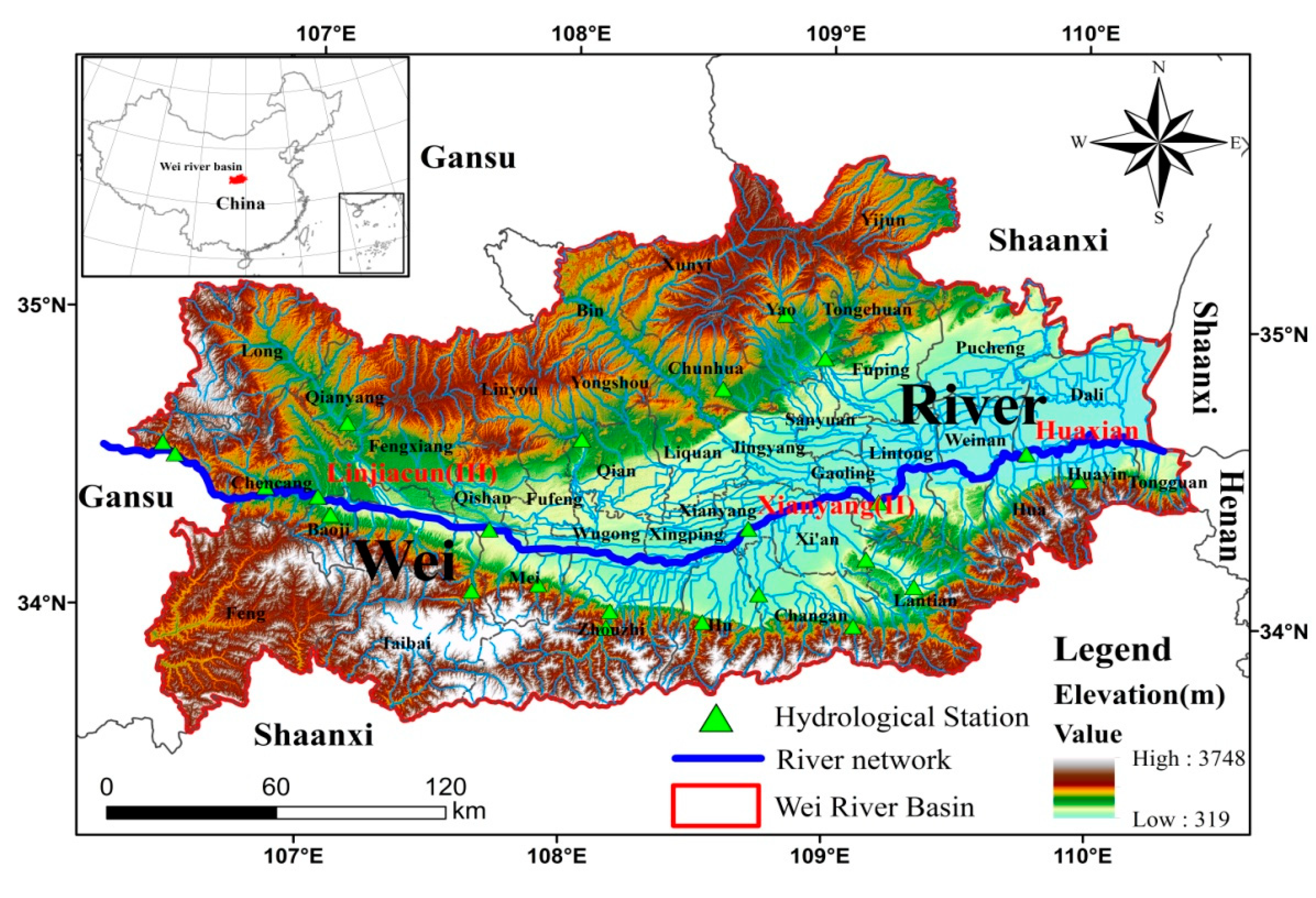
2.1. Study Area

The study area has been shown in Figure 1. The Wei River Catchment lies within the LP and the drainage area is approximately 67,108 square kilometers. The Wei River flows through various types of topography, including hilly and gully regions, terraces, river valley flood-plains, and mountainous earth-rock regions. There is a gradual decrease of terrain from West to the East, with an altitude ranging from 319 m to 3748 m. It is cold and dry during winter and hot and rainy during summer, with an uneven distribution of rainfall. It receives 400–750 mm of annual precipitation on average. The catchment is heavily eroded, and its erosion intensity ranges from extremely heavy to modest light. This is because, based on standards for classification and graduation of soil erosion, the average erosion modulus of 8000~15,000 t/(km²·year), 5000~8000 t/(km²·year), 2500~5000 t/(km²·year), 1000~2500 t/(km²·year) correspond to extremely heavy, serious, modest, and light erosion. The tributaries on the north shore of the Wei River flow through ecologically vulnerable regions where soil is easily eroded with sparse vegetation cover and agricultural production is extensive, as such, transports the most sediment; tributaries on the south shore are better in this respect. Economic growth has put a great burden on water and land resources, causing much soil erosion. The amount of surface water dropped from 63 × 10⁸ m³ in 2005 to 36.75 × 10⁸ m³ in 2015, meanwhile the groundwater resources fell from 57.6 × 10⁸ m³ in 2005 to 40.8 × 10⁸ m³ in 2015 [13]. As of 2015, socioeconomic conditions yielded significant differences among counties. The population density varies from 20 persons/km² to 1220 persons/km² and the population density in downstream areas is larger than that in other parts of the catchment. The grain yield of each sample county falls into the range from 147.13 to 1920.92 kg/person. The per capita GDP of each county ranges from RMB 7338.25 to 75,329.44 [14].

2.2. Control Efficiency Calculation

In this paper, the control efficiency of soil and water loss refers to the ratio of the amount of soil and water loss to the various inputs of treatment measures. The ecological treatment efficiency reflects the actual production and utilization of economic resources, and measures the gap between the actual state of resource allocation and the ideal state of effective allocation. Following the principles of indicator representation and data accessibility, two input indicators were chosen to represent the expenditure of treatment measures, namely, the proportion of restored farmland to forestland/grassland and terraced fields across the entire administrative area (I₁) and the amount of investment in the SLCP and terrace construction (I₂). Additionally, three output indicators were used to characterize the control effects of soil and water erosion, which are average annual runoff (O₁), sediment concentration (O₂), and annual sediment discharge (O₃) (Shown in

Table 1. Input and output indicators of control efficiency.

Variables Type	Abbr.	Variable Definition
Input indicators	I1	Ratio of restored farmland to forest/grass and terraced fields across the administrative area
	I2	The amount of investment in SLCP and terraced construction in each sample county
Output indicators	O1	Average annual runoff
	O2	Average annual sediment concentration
	O3	Average annual sediment discharge

Note: The output index is a reverse indicator, and we use the reciprocal of output indices in the efficiency calculation.

) [7,15,16,17,18,19,20,21,43,44].

The Data Envelopment Analysis (DEA) is widely used for evaluating the effectiveness of decision-making units in light of a multi-input and multi-output model [45,46]. Given the fact that the original DEA method sometimes overestimates the deviation and the bootstrap method can generate a large number of simulated samples, the Bootstrap-DEA model has been introduced to correct estimated efficiency bias and achieve accurate confidence intervals [47,48,49]. Therefore, the control efficiency is measured through the Bootstrap-DEA model in order to acquire a more accurate result. The calculation is conducted by adopting a statistical analysis based on R software. The processes are as follows:

(1)

DEA is used to calculate each county’s (k = 1, 2, …,n) efficiency value ${\widehat{\theta }}_k$, $X_k$ and $Y_k$ represent the input and output of the kth county respectively.

$${\widehat{\theta }}_k=\min \left\{\theta |Y\lambda \ge Y_k;\theta X_k\ge X\lambda ;\lambda \ge 0\right\}$$

(1)

where $\theta$ is scalar, and $\lambda$ is n × 1 dimensional constant vector;

(2)

generate random efficiency ${\theta }_{1b}^{\ast },\dots ,{\theta }_{nb}^{\ast }$, where n represents county, b means iterating b times, ${\theta }_{kb}^{\ast }$ represents the kth random value in the bth interaction, where k = 1, …,n;

(3)

compute estimated sample $\left(X_{kb}^{\ast },Y_k\right)$, where $X_{kb}^{\ast }=\left({\widehat{\theta }}_k/{\theta }_{nb}^{\ast }\right)\times X_k$, k = 1, …,n;

(4)

compute each estimated sample’s efficiency ${\widehat{\theta }}_{bk}$ based on the DEA method, where k = 1,…, n;

(5)

loop over step (2) and (4) for B times. In this paper, 1000 iterations were conducted and the confidence level of 95% was used, thereby generating a 1000 unit dataset to represent the kth random value in the bth iteration. The smooth bootstrap distribution can simulate the original sample estimator and estimate the corrected DEA efficiency deviation:

$$Bias\left({\widehat{\theta }}_k\right)=E\left({\widehat{\theta }}_k\right)-{\widehat{\theta }}_k,$$

(2)

$$B\widehat{i}as\left({\widehat{\theta }}_k\right)=B^{-1}\sum _{b=1}^B\left({\widehat{\theta }}_{kb}^{\ast }\right)-{\widehat{\theta }}_k.$$

(3)

The bias-corrected estimator is presented as follows:

$$\tilde{\theta }={\widehat{\theta }}_k-B\widehat{i}as\left({\widehat{\theta }}_k\right)=2{\widehat{\theta }}_k-B^{-1}\sum _{b=1}^B\left({\widehat{\theta }}_{kb}^{\ast }\right).$$

(4)

2.3. Spatial Data Analysis of Control Efficiency

2.3.1. Global Moran’s Index

The control efficiency varies due to different resource endowments, economic development, geographic location, etc. in different counties. The geographic location of each county can not only affect its own control efficiency, but also influence that of its neighborhoods, that is, the spatial distribution of counties may lead to spatial auto-correlation [41]. In this case, a spatial correlation in control efficiency needs to be estimated. Methods including Global and Local spatial auto-correlation.

Firstly, Global Moran’s Index was used to determine whether there was a spatial correlation in control efficiency. The global Moran’s I value ranges from (−1,1). If I < 0, there is a negative spatial correlation, which indicates that the efficiency in the study area is in a discrete state. If I > 0, there is a positive correlation, indicating an agglomeration state. If I = 0, demonstration is made that the treatment efficiency is random. The calculation is presented as follows:

$$I=\frac{n{\displaystyle \sum _{i=1}^n{\displaystyle \sum _{j=1}^n{w}_{ij}}}\left(x_i-\overline{x}\right)\left(x_j-\overline{x}\right)}{{\displaystyle \sum _{i=1}^n\left(x_i-\overline{x}\right){\displaystyle \sum _{i=1}^n{\displaystyle \sum _{j=1}^n{w}_{ij}}}}}$$

(5)

where n represents the total number of counties; x_i and x_j shows county i and county j’s control efficiency; $\overline{x}$ represents the average control efficiency; and $w_{ij}$ is the spatial weight matrix, which can be constructed according to the Queen and Rook Spatial Weight matrix.

2.3.2. Getis-ord G_i^* Index

Compared with the global spatial autocorrelation, the Getis-ord G_i^* Index not only determines high- and low-value agglomeration accurately, but also displays sub-high and sub-low areas, allowing for a complete expression of transitional geospatial information [50,51,52]. The Getis-ord G_i^* Index assumes a normal distribution and is calculated as follows:

$${G_i}^{\ast }=\frac{{\displaystyle \sum _{j=1}^n{w}_{i,j}{x}_j-}\overline{x}{\displaystyle \sum _{j=1}^n{w}_{i,j}}}{S\sqrt{\frac{\left[n{\displaystyle \sum _{j=1}^n{w}_{i,j}^2-{\left({\displaystyle \sum _{j=1}^n{w}_{i,j}}\right)}^2}\right]}{n-1}}},\overline{x}=\frac{{\displaystyle \sum _{j=1}^n{x}_j}}{n},S=\sqrt{\frac{{\displaystyle \sum _{j=1}^n{x}_j^2}}{n}-{\left(\overline{x}\right)}^2}$$

(6)

where $x_j$ represents the treatment efficiency of soil erosion in county j. $w_{i,j}$ is the spatial weight between county i and j; n represents the amount of samples; $\overline{x}$ represents the average treatment efficiency; S is the standard deviation of treatment efficiency. $G_i^{*}$ records z’s score, where in the higher the z value, the tighter the clustering of high values (hot-spots); likewise, the lower the z value, the tighter the clustering of low values (cold-spots). A z value close to zero indicates that there is no spatial cluster.

2.4. Influencing Factors of Control Efficiency based on the Spatial Statistic model

2.4.1. GWR Model

The relationship and structure of variables change with geographic location, resulting in the spatial non-stationarity and heterogeneity of each decision-making unit [53]. Therefore, the introduction of spatial location elements into a linear regression model can help to quantify this spatial heterogeneity. In 1996, Fotheringham et al. [41] introduced the GWR model, the central idea of which was to take the geographic location as an important parameter for global model parameter estimation. The model delimits an appropriate local window for calculating the attenuation function and then reinserts the calculated weight value back into the regression equation [54]. In this regard, the GWR model has been widely used in spatial correlation studies [55,56,57,58]. The function is as follows:

$$E_i={\displaystyle \sum _{j=1}^n{\beta }_{ij}(u_i,v_i)x_{ij}}+{\epsilon }_i,j=1,2,3,\dots ,n$$

(7)

where $E_i$ is the observation value of governance efficiency in county i, $x_{ij}$ is the explanatory variables (j = 1, 2, 3, …,n), ${\beta }_{ij}(u_i,v_i)$ is $x_{ij}$’s co-efficiency, $(u_i,v_i)$ is the latitude/longitude coordinates of sample i, and ${\epsilon }_i$ is the independent and identically distributed random error.

During the solution process, we used the Gauss form to set the weight and the cross validation (CV) of local regression analysis to set the bandwidth (b₀); the equation is as follows:

$$CV={\displaystyle \sum _{i=1}^n{[y_i-y_{\ne i}(b_0)]}^2}$$

(8)

where $y_{\ne i}(b_0)$ is the fitted value of sample i. When the CV reaches the minimum, the corresponding b₀ is the optimal bandwidth. As different spatial weighting functions obtain various bandwidths, many researchers have adopted the calculation criterion proposed by Hurvich et al. [59], which indicates that when AIC (Akaike Information Criterion) reaches the minimum, the corresponding b₀ is the optimal bandwidth.

2.4.2. The Selection of Influencing Factors

Based on previous studies concerning the construction of GWR models, treatment efficiency was used as the dependent variable. In reality, the estimation of the improvement of control efficiency with multiple indicators involved is more effective and corresponds with the theoretical framework. For the independent variables, to achieve the non-multicollinearity in the GWR model, six indicators, namely, the ratio of shrub-grass area, slope, precipitation, per capita GDP, per capita grain production, and population density were finally chosen after a series of statistical tests. Detailed information has been shown in

Table 2. Description and explanation of influencing factors of control efficiency.

Variable Definition	Abbr.	Unit	Excepted Sign
Ratio of sum areas of shrubs and grasslands to the administrative area	cover	%	+
Average slope of each sample county	slope	°	-
Average annual precipitation	prep	mm	-
Per capita GDP	pgdp	Yuan	+
Per capita grain yield	pgrain	t	+
Population density of each sample county	density	person/km2	-

Note: “Grain production” here denotes the production of food crops throughout the whole society, including rice, wheat, corn, sorghum, millet, miscellaneous grains, potatoes and beans.

.

These indicators were chosen for the following reasons:

(1) The ratio of summed areas of shrubs and grasslands to the administrative area, which represents differences in land-use patterns may also affect the degree of soil and water loss reduction. Concerning the characteristics of the hydrothermal soil factors of the LP, shrub-grass has better soil and water conservation effects than that of arbor-lawn [60,61]. Therefore, the areas which have higher proportions of shrub-grass, less investment, and restored areas may produce higher soil and water reduction; in other words, the control efficiency is likely to increase. Therefore, the ratio of sum areas of shrubs and grasslands to the administrative area is expected to have a positive effect on control efficiency.

(2) Precipitation and slope are used to reflect the impact of local precipitation and topographical conditions on the control efficiency for soil and water erosion management. Precipitation and slope contribute most to soil erosion in the LP [62]. The higher the annual rainfall in obviously eroded areas, the stronger the runoff and its sediment-carrying capacity in rivers, which significantly affects the output and lessens the efficiency of treatment. Therefore, it is expected that the impact of precipitation and gradient is negative, given that the steeper the slope, the more difficult it is to control soil erosion.

(3) Population and economic factors represent the impact of population density levels and socio-economic development on control efficiency, which are characterized by population density and per capita GDP, respectively [63,64]. Growth in population size exacerbates resource exploitation, especially on non-agricultural land and impervious land which affect both runoff and sediment production. Therefore, population density is expected to produce a negative impact on control efficiency. In more developed regions, people tend to have high expectations for their living environment. In this sense, with other input conditions constant, more advanced technologies, greater manpower, and more funding will ensure a higher output and better efficiency. Therefore, GDP per capita is expected to have a positive impact on efficiency.

(4) Agricultural production is measured by per capita grain yield. The land, which is not suitable for agricultural development, such as steep slopes, is turned into ecological land. However, the land suitable for agricultural development is intensively managed. The land management strategy not only improves the treatment efficiency, but also contributes to the agricultural land conservation and food production. Therefore, the impact of per capita grain yield on the control efficiency is expected to be positive [65,66].

2.5. Data Collection and Processing

On the basis of the vegetation-based soil and water conservation mechanism and the hysteresis of rainfall-infiltration-runoff, there exists a time lag of the projects, and a cross section of every four years was selected [43,67,68]. The years 2005, 2010 and 2015 were used as the time frame.

The data concerning runoff, sediment concentration, and discharge were collected from the Annual of Hydrological Data of the Yellow River Basin (2001–2016). Moreover, the data on investment and the area of terraced fields were collected from the Shaanxi Provincial Water Statistics Yearbook (2001–2016). The annual data on the implementation of the SLCP were provided by the Shaanxi Province Forestry Department (1999–2015). The socio-economic data of the 39 counties in the present paper were from the China City Statistical Yearbook (2001–2016) and the China County Statistical Yearbook (2001–2016).

In addition, the data on land-use types came from the Center for Resources and Environmental Sciences of the China Academy of Science with 30 m resolution [69]. This dataset was generated by artificial visual interpretation. In accordance with field verification and error correction, the evaluation accuracy of the primary and secondary land-use types reached 94.3% and 91.2% respectively, suggesting a high level of accuracy (Verification method: using the same data source, we randomly and evenly collected sample area on the images, and ensured that each land-use type should be selected. After all the selected sample areas were interpreted, the results would be compared to the original results, and we then obtained the error rate of interpretation [70]). The land-use classification criterion was provided by the China Academy of Science.

Geographically, the water runoff and sediment data were collected through a multistep process. Precipitation data were collected from 50 meteorological stations in and around the Wei River Catchment and were used together with the dataset from the China Meteorological Administration; it had a resolution of 1 km [71]. Water and soil data were obtained from 40 hydrological observation sites in the Wei River Catchment (The hydrological observation sites included 24 sites in the study area, and 16 sites outside the study area. We doing so by adding more controlling points in order to increase the interpolation result’s accuracy). The latitude and longitude of each observation site were imported into the ArcGIS10.2 (ESRI, Redlands, CA, USA) under the WGS_1984_UTM_zone_49N spatial coordinates. Gradient calculations were conducted based on the DEM and determined by the slope function provided by Spatial Analyst. Finally, the study employed the Tabulate Area Tool to account for the elevation, as well as the spatial distribution of gradients of each land type. The tool was also used to calculate the average gradient, annual precipitation, runoff, sediment concentration, and sediment transport for each county according to the administrative division. Vector data about the 39 administrative districts came from the national 1:1,000,000 database of the National Fundamental Geographic Information System [72].

3. Results

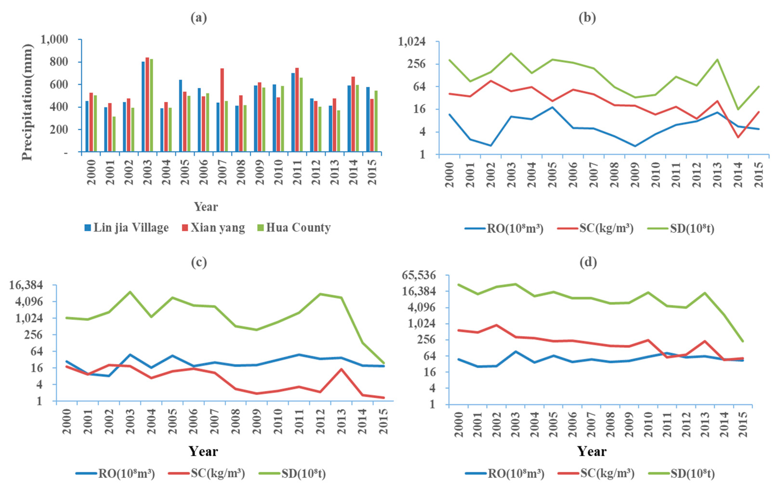
3.1. Analysis of Inter-annual Fluctuation Trends of Runoff, Sediment Concentration and Discharge, and Precipitation

To analyze the inter-annual fluctuation of runoff, sediment concentration, and discharge and precipitation, the data from three hydrological stations, namely, Lin Jia Village, Xian Yang, and Hua County were used. These stations were chosen for their geographic appropriateness and capacity to yield relevant data. The observation station in Lin Jia Village is situated in the upper- and middle-reaches of the Wei River; the station in Xian Yang resides in the middle- and lower reaches; and the station in Hua County serves as an exit where the Wei River outflows from Shaanxi province to join the YR [73].

Considering that there is a lag period of 4–5 years for vegetation to bring ecological benefits into play and the minimum precipitation period of 5–6 years, the whole research is divided into three periods: 2000–2005, 2005–2010 and 2010–2015 [43,67,68,74]. The inter-annual variations of precipitation, runoff and sediment are analyzed. Figure 2a shows that there is little difference in annual rainfall among the three hydrological stations, the rainfall value fluctuates between 400 and 600 mm, and the year when the extreme value occurs is relatively uniform. In addition, during the process of catchment and sediment collection from upstream to downstream, the runoff and sediment indices of the three stations are significantly different.

Lin Jia Village Station: Compared with the mean value of years 2000–2015, the variation ranges of the mean value of rainfall in the three periods are −1.86%, 2.15% and 5.32%, respectively, those of runoff are 30.23%, −10.18%, and 0.15%, respectively, those of sediment transport 49.62%, −9.19%, and −37.69%, respectively, and those of sediment concentration 56.43%, 12.37% and 58.07%, respectively.

Xian Yang Station: Compared with the mean value of years 2000–2015, the variation ranges of the mean value of rainfall in the three periods are −2.61%, 1.06%, and −1.23%, respectively, those of runoff −3.71%, −0.44%, and 0.86%, respectively, those of sediment transport 25.66%, −19.14%, and −21.74%, respectively, and those of sediment concentration 62.86%, −14.56%, and −53.61%, respectively.

Hua County Station: Compared with the mean value of years 2000-2015, the variation ranges of the mean value of rainfall in the three periods are −2.93%, 1.09% and 4.41%, respectively, those of runoff −2.34%, −4.42%, 3.01%, respectively, those of sediment transport 69.52%, −16.99%, and −44.31%, respectively, those of sediment concentration 76.84%, −24.44% and −55.78%, respectively.

3.2. Measuring Control Efficiency

As stated above, the Bootstrap-DEA was used to calculate the control efficiency for soil and water loss in the Wei River Catchment of the years 2005, 2010 and 2015. Appendix A lists the efficiency values measured by DEA and Bootstrap-DEA, and the bias values between these two methods in 2005. The Column 5 (Lower bound) and 6 (Upper bound) represent the confidence intervals. Values measured by DEA are all beyond the confidence intervals. In other words, the outcome computed by DEA is overestimated and will not be accepted, and thus, only the outcomes calculated by Bootstrap-DEA were presented for 2010 and 2015 and were used for further analysis [47,48,49].

It could be found form results that the average ecological control efficiency increased from 0.263 to 0.365 within the research site and numerically the efficiency was relatively low with a significant difference. In the aspect of spatial distribution, the control efficiency of counties, located in the upper- and middle reaches, was generally higher than that of downstream counties and the efficiency at the southern bank of the river was much better than that at the northern bank. In an attempt to analyze the dynamic change of counties’ control efficiency, the control efficiency is divided into five types in the present study and the results are shown in Figure 3. In 2005, altogether there were 35 counties with the control efficiency less than 0.4, accounting for 89.64% of the total samples, while the counties with control efficiency above 0.6 were Baoji County, Qian County and Xingping County. In 2010, the number of counties with control efficiency below 0.4 dropped to 10 and the efficiency presented an increasing trend in Qianyang, Taibai, Long and Feng counties in Baoji City, Zhouzhi, Hu and Changan counties in Xi’an City, Yongshou, Qian and Wugong counties in Xianyang City, as well as Yao County in Tongchuan City. In terms of numerical and spatial distribution, there was no significant difference between the year 2010 and 2015 in the control efficiency. In general, the number of counties entering the high-efficiency class is increasing, but the overall efficiency of the study area is still at a low level.

In light of the existing research findings, the efficiency value can be divided into technical efficiency and scale efficiency, which contributes to the analysis of the reasons for the change of control efficiency. The commonly used method is DEA’s Malmquist productivity index method [75]. The Malmquist productivity index is calculated based on the control efficiency of two periods. The pure technical efficiency indicates the level of resource allocation restricted by a specific production technology; the scale efficiency reflects the scale aggregation efficiency of resource inputs. Therefore, it is of great importance to analyze in-depth efficiency changes in terms of both factor allocation and the scale of agglomeration.

Appendix B shows the changes at county level for the aforementioned Malmquist productivity index in 2005, 2010 and 2015. We define 2005–2010 and 2010–2015 as the first and second phase, respectively (Figure A1a,b). “MI”, “pech”, and “sech” correspond to Malmquist productivity index, pure technical efficiency, and scale efficiency respectively. All three indices have a dividing line of 1. When the index is greater than 1, it indicates that the efficiency has increased; if it is less than 1, the efficiency has decreased. The overall trend demonstrates that the decomposition index of each county differs significantly. In the first phase, 25 counties had a pure technical efficiency greater than 1 and 17 counties had a scale efficiency greater than 1, which signified that 25 counties were technically efficient, and 17 counties were effective on scale. Compared with the first phase, from 2010–2015, the number of counties with increased scale efficiency presented a significant growth, and the proportion of total samples rose from 43.59% to 61.54%. However, the number of counties with technically effective showed a downward trend, from 64.1% to 47.13%. During the years 2005–2010, the change in trend of technical efficiency was similar to the fluctuation of the Malmquist productivity index in terms of variation tendency, while the trend of scale efficiency in 2010–2015 was more closely related to the fluctuation of the Malmquist productivity index. In this regard, the growth of control efficiency in the early stage mainly depended on the increase of factor input, while the scale effect exercised a significant influence on the growth in the later stage.

3.3 The Spatial and Temporal Pattern Evolution Characteristics of Control Efficiency

Owing to the difference in the policy implementation intensity of counties and resource endowment condition, the regional economic growth dependency presented a growing tendency and the technological diffusion allowed different regions to absorb neighboring experience, which would eventually bring about the convergence or spatial convergence of geographical space, that is to say, there was a strong correlation between a region and its adjacent areas in the social and economic development, although the correlation was affected by spatial distance and resource endowment conditions at the same time [76]. Based on the previous calculation value of control efficiency and the calculation results after decomposition, the spatial statistical inference method is adopted to verify the spatial agglomeration among counties in the study areas. The commonly used methods include global spatial autocorrelation and local spatial autocorrelation.

3.3.1. Overall Spatial Pattern Evolution Characteristics

Moran Index is a commonly used indicator for global spatial autocorrelation. The index is often employed to verify the relation of ecological management efficiency to spatial distribution and reflect the relevance of control efficiency in different spatial locations, which serves as a measurement of the spatial agglomeration degree of control efficiency in each county.

GeoDa software was used to calculate the Global Moran’s Index of treatment efficiency in 2005, 2010, and 2015. Results have been shown in

Table 3. Results from Global Moran’s Index.

Index	2005	2010	2015
Moran’s Index	0.192	0.134	0.151
z-value	2.295	1.663	1.746
p-value	0.022	0.094	0.081

Note: p values of 0.01, 0.05, 0.1 mean that the result is randomly generated of 1%, 5%, 10% possibilities. The z value is the multiple of the standard deviation; when the z value < 1.65, the pattern appears to be random.

. As the calculation results indicate, the Moran Index for water and soil loss in each county were 0.192, 0.134 and 0.151, respectively, from 2005 to 2015. In 2005, the random distribution, at most, accounted for 5% of total data distribution concerning the control efficiency for water and soil loss and the possibility of spatial unit accumulation was greater than that of random distribution, with significant rejection of the null hypothesis. Given the z-value of 2.295, there was a less than 5% likelihood that this clustered pattern could be the result of random chance. In the years of 2010 and 2015, less than a 10% likelihood fell into random distribution. The possibility of spatial unit aggregation was greater than that of random distribution and could obviously reject the null hypothesis. The results indicated that the spatial distribution of control efficiency in each county, with a positive spatial correlation mode, had some clustering characteristics, but the global correlation was still at a low level.

However, the global Moran Index reflects the potential interdependence of all unit elements in a general spatial range, which cannot verify the concentration of local unit elements. Therefore, local spatial autocorrelation can be used for verification.

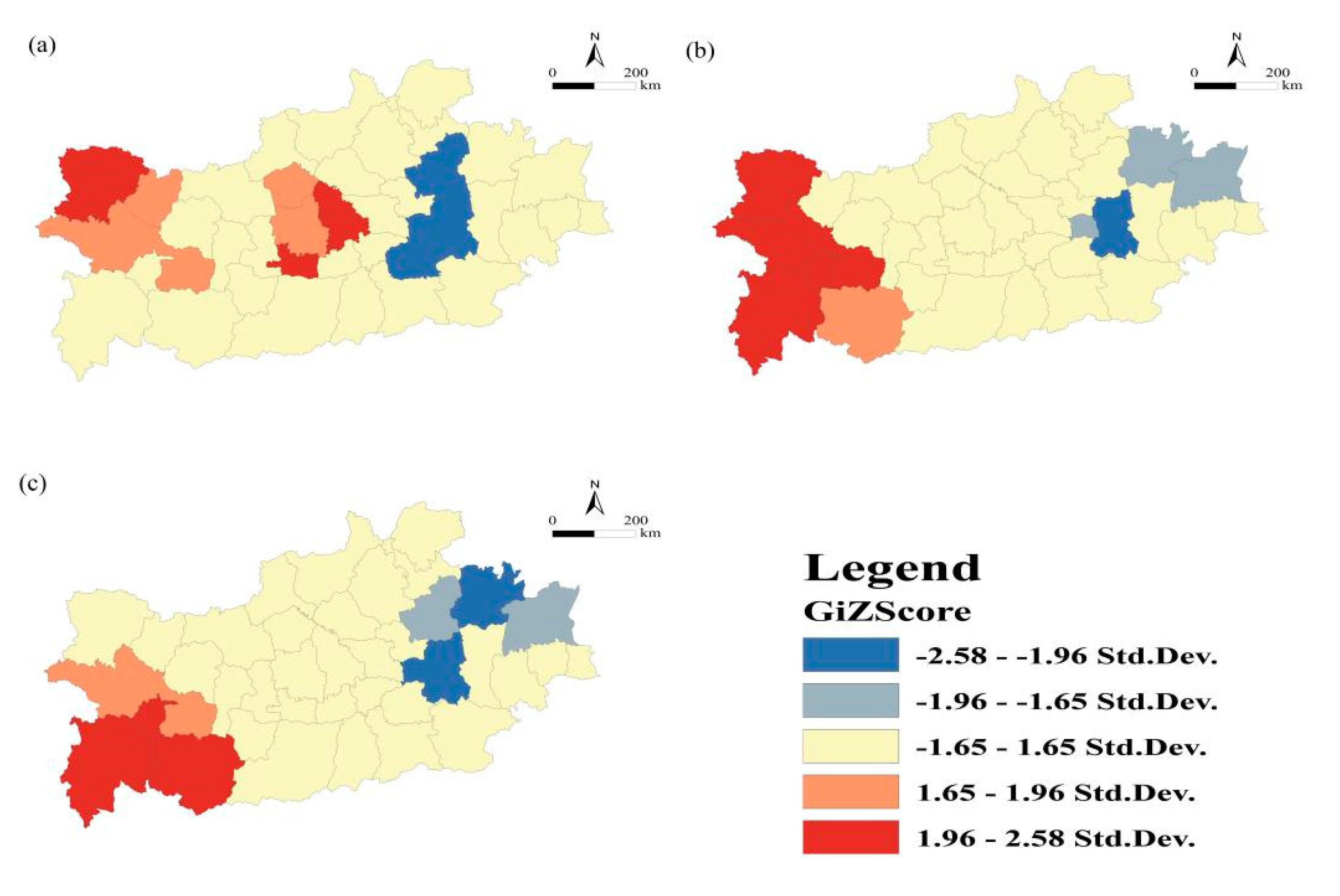
3.3.2. Local Spatial Pattern Evolution Characteristics

Hot-spot analysis is commonly used in local spatial autocorrelation analysis, which describes the similarity between any spatial unit and its adjacent units and reflects how the similarity changes with time and position. With the help of this analysis tool, it is easy to identify the time and location of hot spots (areas with high control efficiency) and cold spots (areas with low control efficiency) with statistical significance, and to aid decision makers to allocate resources reasonably in time.

By employing the hot-spot method of analysis, we divided the local index into five distinct types: cold spot areas, sub-cold spot areas, sub-hot spot areas, hot spot areas, and insignificant areas [54]. As shown in Figure 4, in 2005, there were three hot spots of control efficiency, namely, Long County in Baoji City, Liquan County, and Wugong County, with a radius extending to Yongshou and Qian Counties. The cold spot center was Lintong, the radius of which extended to the municipal districts of Xi’an, Gaoling, and Fuping. In 2010, the hot spots of control efficiency mainly focused on the counties in Baoji City. The cold spot area, compared with 2005, clustered in Lintong, Gaoling, Pucheng and Dali counties. By 2015, the hot spot had moved to Taibai and Feng counties in Baoji City, while the cold spots remained stable and thus unchanged. From the perspective of spatial location, the hot spots were mainly located in the upper reaches of the study area, while the cold spots centralized in the downstream area, the counties where two tributaries of Jing River and Beiluo River were remitted into the main stream of Wei River.

3.4. Factors Affecting the Spatio-temporal Changes of Control Efficiency

With regard to the counties in the upper reaches of Wei River (mainly include Long, Baoji, Feng, Taibai, Fengxiang, Linyou, Qishan and Mei counties in Baoji City), there is a slight difference in the input and output of each county for soil and water loss; but the control efficiency greatly varies, since the natural endowments and socio-economic environment differs in different counties and the relationship among variants changes with geographical location. Therefore, the GWR model can better solve the problem of spatial heterogeneity. As Zhang [77] states, “the idea of local regression is entailed in the GWR model with a set window. All the samples in the local window are weighted according to their distances from the corresponding current point, while the samples outside the local window are weighted as 0 and the regression coefficients can be estimated based on the samples in the current local window at the time, which is centered on the current point.” The estimation coefficients of each variable, contained in the model, means the contribution of each independent variable to the ecological control efficiency. Finally, the results estimated by GWR can be used for policy adjustment. GWR4.2 software was adopted to conduct the results for a GWR model. Results of the regression are shown in

Table 4. Regression coefficient of geographically weighted regression (GWR) from 2005–2015.

Variables	2005	2010	2015
lnintercept	−1.91~−1.5207 ***	−1.55~−1.05 ***	−1.39~−1.24 ***
lncover	0.17~0.39 **	0.050~0.120	0.170~0.23 *
	(0.22)	(0.06)	(0.20)
lnslope	−0.32~0.01	−0.42~−0.20 *	−0.32~−0.15 *
	(−0.09)	(−0.26)	(−0.25)
lnprep	−0.17~0.01 *	−0.01~0.36	0.40~0.55 ***
	(−0.12)	(0.12)	(0.49)
lnpgdp	1.83~13.12 *	−2.45~2.31	−1.18~1.51
	(7.14)	(−1.72)	(−0.82)
(lnpgdp)2	−13.48~−2.18 **	1.14~2.44	0.47~1.48
	(−7.51)	(1.77)	(0.65)
lnpgrain	0.16~0.33 *	0.01~0.20	0.05~0.68 **
	(0.25)	(0.10)	(0.43)
lndensity	−0.46~−0.24 **	−0.77~−0.25 ***	−0.90~0.01 **
	(−0.35)	(−0.53)	(−0.60)
bandwidth	100	90	90
AICc	104.60	118.31	104.78
R2	0.58	0.50	0.63
Adjusted R2	0.36	0.28	0.42
GWR Residuals	15.18	16.43	11.87
Global Residuals	17.94	25.50	16.42

Note: ***, **, and * denote statistical significance at 1%, 5%, and 10%, respectively. The GWR model can simultaneously estimate the regression coefficient of each sample county across factors to determine the control efficiency. Taking “lncover” as an example, “0.17~0.39” indicates the effect which the coefficient of grass-shrub cover has on the control efficiency of each sample county. Numbers in parentheses are the mean coefficients of the total sample. We adopted the price index from 2000 as the base year to calculate the per GDP index in the three periods for comparable conversion.

. All the visualized variable coefficients of control efficiency are shown in Appendix B. Based on multiple attempts, the optimized bandwidth was determined as 90 km.

3.4.1. The Impact of Proportion of Shrub-grass Area Effect on Control Efficiency

The results indicate that shrub-grass has a positive effect on control efficiency. When the proportion of shrub-grass increases by 1%, the control efficiency improves by 0.20–0.22%. The proportion of shrub-grass in the study area increased from 13.23% in 2005 to 31.42% in 2015. Based up on the regression coefficients, counties in the upper and middle reaches were greatly affected by the proportion of shrub-grass area over the administrative area. In the early stage of treatment, the increase of shrub-grass cover in the upper and middle reaches effectively prevented soil erosion and conserved soil and water resources. As time passed, healthy vegetation cover in the downstream areas helped to reduce sediment, which in turn increased the control efficiency. In terms of spatial distribution, there was an overlap between areas with a high proportion of shrub-grass and high control efficiency for soil erosion, indicating that the structure of shrub-grass is fundamental to the spatial distribution of control efficiency.

3.4.2. The Impact of Slope and Precipitation on Control Efficiency

Results show that the impact of the annual average rainfall on control efficiency in 2005 and 2015 was statistically significant at 10% and 1% respectively. The effect of slope on control efficiency in 2010 and 2015 was statistically significant at 10%. The facts stated above demonstrate that these two factors play an important role in how to improve the control efficiency. The mean regression coefficient shows that the annual rainfall coefficients for 2005, 2010, and 2015 were −0.122, 0.115 and 0.49, respectively, and that the average gradient coefficients were −0.09, −0.26 and −0.25, respectively. These results indicate that, in 2005, for every 1% increase in the average annual precipitation there was a 0.12% reduction in control efficiency. In 2015, a 1% increase in the average annual precipitation resulted in a 0.49% increase in control efficiency; while when the slope grew by 1%, a 0.25% reduction is displayed in control efficiency. Furthermore, in 2005, the impact of precipitation was concentrated in the upstream counties. In 2015, the impact center shifted to counties located in the middle region.

3.4.3. The Impact of Per Capita GDP on Control Efficiency

The impact of per capita GDP on control efficiency varies across years. A quadratic term was added to examine whether there is a nonlinear relationship between per capita GDP and control efficiency. The results show that in 2005 the relationship between them fits the inverted “U”-type Kuznets curve. This means that the counties on the left side of the inverted “U” curve have the same per capita GDP and efficiency. A 1% increase in per capital GDP led to a 7.14% increase in treatment efficiency. In 2010 and 2015, the linear and quadratic term coefficients of per capita GDP were not statistically significant. Moreover, the linear term coefficient was negative, indicating that, to some extent, socio-economic improvements can help restore the environment through strong investments in treatment.

3.4.4. The Impact of Per Capita Grain Yield on Control Efficiency

In 2005 and 2015, per capita grain yield had a positive and statistically significant impact on control efficiency. A 1% increase in grain yield resulted in a 0.25–0.43% increase in control efficiency. In terms of spatial distribution, the areas with higher grain yields were primarily distributed in the downstream areas near the trunk stream and tributaries of the Wei River. In spite of the not high control efficiency in these areas, it is important to note that these are the catchment areas for each tributary. They are systematically cultivated to reach large-scale production, that is, to transform extensive production into intensive production, which not only ensures adequate food supply, but also improves control efficiency.

3.4.5. The Impact of Population Density on Control Efficiency

The impact of population density on control efficiency is statistically negative. Estimation results show that an increase of 1% in population density results in a reduction in control efficiency by 0.35–0.60%. Coefficients from the downstream areas in the main stream and tributaries of Wei River are significantly higher than those in the upper and middle areas, indicating that areas with a high population density have a low control efficiency, since these areas are usually accompanied by high-intensity production and living activities, which are characterized by large areas of non-agricultural land and low vegetation coverage.

4. Discussion

Considering the complicated process of soil and water loss, a preliminary descriptive data analysis from three main observatories was conducted concerning whether human interventions can exert influence on such processes, which lay the foundation for calculating and analyzing the control efficiency. As Figure 2 indicates, in general, the annual amounts of rainfall and runoff are fluctuating, and since 2005, the increase/decrease rate in runoff is less than that in rainfall. The sediment transport and sediment concentration displayed a significant and continuous downward trend; compared with that in the period of 2005–2010, the amount of sediment in the period of 2010–2015 decreased by a multiple of 1.98. In other words, this chart is a nice tie-in with human interactions, which shows the importance for control efficiency analysis.

The state-led projects like the SLCP have played a positive role in soil and water reduction in the Wei River Catchment, and our empirical results show that the control efficiency of treatment measures dealing with soil and water loss is still low. There are some reasons for the current situation. On the one hand, the primary objective of the SLCP is to solve serious soil erosion problems by restoring vegetation. Owing to the urgency to protect the ecological environment, the adaptability of planted vegetation to the local area was neglected in the initial stage of the project, which led to the almost zero survival rate of the first batch of vegetation and no improvement in the ecological environment despite a large amount of investment [78]. On the other hand, the SLCP is mostly implemented in areas with poor land quality in the Shaanxi Province, and the average amount of compensation per mu (Mu is a Chinese measure of land area, which one mu is 1/15 of a hectare) for planting trees and grass is about 2 times or more than the opportunity cost, which means the net revenue from grain production before being enrolled in the program [37]. At the same time, in Northwest China, the ecological benefits of planted vegetation are far less than the original vegetation before deforestation. Therefore, such kind of overcompensation can help alleviate the local poverty, but in the case of high input and low output, there is still much room for the improvement in the control efficiency for soil and water loss [79]. In addition, according to two articles of Zhang [80,81], the blurred boundary between the industrial and ecological margins of forestry in China dampens the enthusiasm of local forestry producers for afforestation, and the government have to bear the responsibility of afforestation; in such a context, the fact not only increases the afforestation burden of the central finance, but also leads to the unfavorable ecological benefit as a result of inadequate management and protection. With the time going by, the possible reason for the improvement of the efficiency of ecological management is that on the one hand, the funds invested are gradually diversified [36]; on the other hand, the ecological benefits of natural succession of vegetation are gradually increasing.

As the spatial distribution of control efficiency shows, the control efficiency of counties in the lower reaches of the Wei River is relatively low. The possible reasons may be as follows. On one hand, Jing River and Beiluo River, the two main tributaries of the Wei River, are the main sources of sediment in the Wei River; the Jing River finally flows through Gaoling County and Lintong County to the Wei River, and the Beiluo River finally runs through Pucheng County and Dali County to the Wei River. Despite a little decrease of sediment after treatment, compared with other counties, most the runoff and sediment from the upper and middle reaches are concentrated in the Pucheng County and Dali County, resulting in the great pressure on the ecological environment. On the other hand, as Appendix B demonstrates, the counties with low control efficiency are characterized by a low proportion of shrub grass and the average annual precipitation in the downstream counties is slightly higher than that in the upper reaches. Additionally, the economic growth leads to the exploitation of ecological land by non-agricultural land. These factors affect the improvement of ecological control efficiency.

The result of the hot-spot analysis displays the position of the hot-spots and cold-spots changing with time. The possible explanation are as follows: firstly, the intensity of investment varies with the stage of implementation of the project [82]; secondly, the comprehensive results are affected by the geographical location and socioeconomic factors. Besides, the hot spots and cold spots present local agglomeration effect and all the clustered counties belong to the same prefecture level city, where the border effects exist. The existence of the border effects indicates that regions at the border show their bias, as they are not surrounded by regions in the center. In the meanwhile, the counties under the jurisdiction of the same prefecture level have a higher degree of similarity in policy implementation and technology management.

As shown in Table 4, the overall impact of precipitation on the control efficiency in 2005 was significantly negative. Hydrological records show that in 2005, the annual average precipitation in the study area is nearly 10% over the average of many years and there were 3 large-scale rainstorms this year [8]; precipitation has a significant negative impact on the ecological control efficiency considering the short construction period of ecological engineering, lower vegetation coverage and less ecological benefits of water and sediment interception. However, the overall impact of precipitation on the efficiency in 2010 was nonsignificant. In addition to Feng County in Baoji City, Yongshou, Qian, Wugong and Chunhua counties in Xianyang City, Zhouzhi County in Xi’an City, the annual average rainfall has a significant positive impact on the control efficiency of these counties. According to the statistics in 2010, the annual precipitation in Linjia village site and above it was about 8% over than the annual average; the annual average rainfall on the South and North banks below the site was about 10% more than the annual average [8]. After 10 years of natural succession, the ecological effects of vegetation in the upstream region are obvious. Far from increasing runoff and sediment transport, the dry rainfall promotes the growth of shrub and grass vegetation as a natural recharge. In 2015, the overall impact of precipitation put pressure on the control efficiency. The reason is that the average annual rainfall is more than 2–4% than that of many years [8]. The proportion of the shrub grass area to the administrative area increased from 7.49% in 2000, to 16.58% in 2015 [69]. The significant role of vegetation in soil conservation and water storage helps to enhance the ability to resist floods caused by heavy rain, and the ecosystem of the basin can be restored to a certain extent in a period of time. Thus, the increased control efficiency in 2015 suggests that the WSCP and SLCP have made a moderate contribution to controlling soil erosion. Meanwhile, during the whole period, the slope coefficient on efficiency saw a gradual decrease. A reason for this may be that more intensive ecological construction is required in the case of steep slopes, which means more funds and land have to be invested and low control efficiency is demonstrated in these counties.

Drawing on the theoretical framework, the research team also discussed and quantified the factors influencing the control efficiency. Taking Baoji County as an example, an interesting finding has shown there is a non-linear relationship between per capita GDP and the control efficiency (verified introducing a quadratic term). After calculated by equations, once the per capita GDP exceeds RMB 8875, it will pose a negative impact on the control efficiency. We take this case to illustrate that the difference in control efficiency is the result of a combination of multiple factors; the factors affecting control efficiency vary across counties, indicating that regional governments should consider full-scale initiatives. Furthermore, the contribution of per capita grain yield to control efficiency shows a positive impact. Based on the statistical data, from 2000 to 2015, the proportion of cultivated land decreased from 30.60% to 27.95%, while the per capita grain output increased from 481.43 kg/person to 1256.03 kg/person, which indicated that the technological progress contributed to the decrease of arable land and exponential increase of grain yield; in addition, the conversion of marginal farmland with poor land quality into ecological land could reduce soil loss without affecting the grain yield, which had a significant effect on improving the ecological management efficiency [83].

Our research focused on the scientific quantification of the control efficiency of soil and water loss, as well as the factors influencing such efficiency rather than the depiction of the complex process of soil and water loss. For instance, a rainstorm can easily increase the runoff, and then a large amount of sediment transport appears, which will put much pressure on the control efficiency. Besides, future researches are still needed to explore such alternative factors and their cross-correlation effect on how they may or may not affect control efficiency. Other programs, such as the Natural Forest Protection Project where the destruction of vegetation by human activities is prohibited, are considered to be important references insofar as sufficient data are available. What’s more, since the SLCP has only been in operation for 16 years, data tracking is necessarily required to obtain desired outcomes. Finally, the present paper only deals with 39 counties running through Shaanxi province in consideration of the data accessibility principle. Although the data can meet the research needs of this paper, the relatively small number of samples results in a low level of global spatial autocorrelation. In terms of the calculation of control efficiency, the output indicator selected in this paper is the improvement degree of ecosystem service function caused by the increase of forest and grassland area, namely the change of runoff, sediment content and sediment transport; the lag effect and cumulative effect of forest and grass on ecological benefits leads to the lag analysis in this paper [37,84]; however, since our existing technological capabilities cannot measure the growth function of forests and grasses, we can only assume a fixed average value of ecological effects exerted by forests and grasses. The GWR model aims to decide the optimal bandwidth, and the calculation of bandwidth depends on the construction of spatial weight matrix, that is, different spatial weights and related algorithms, which contributes to the different results of bandwidth [85,86,87]. At present, no attempts have been made in determining which calculation method can bring more robust calculation results.

5. Conclusions

To solve the ecological environment issues in an effective and sustainable way, it’s necessary to build a bridge between ecologists and socioeconomic researchers, since ecosystem productivity and stability have an effect on environmental changes [88]. To date, few studies have integrated ecology and socioeconomic disciplines in a real sense. Therefore, our empirical results confirm and highlight the importance of control efficiency estimation in state-led programs concerning ecological issues. Firstly, an interdisciplinary approach was used to overlap the Wei River vector layer and administrative vector layer of local counties. From the perspective of ecological effectiveness, economics and statistical methods were adopted to tie the investment and the expected ES, in order to quantify the PES restoration programs in terms of efficiency. Secondly, geospatial tools were used to interpolate multisource statistical data for annual observation of each county, which helped facilitate subsequent modeling. Finally, socioeconomic conditions and biophysical indicators were integrated into the same analytical framework so that marginal contribution of each independent variable to the ecological control efficiency can be well estimated over time and space.

In theory, to evaluate the control efficiency of the SLCP and WSCP will help enrich and improve the evaluation system of ecological restoration projects. Moreover, matching indicators from different disciplines to build models for quantitative analysis, which is a novel methodology to integrate social and environmental processes, helped to make up the shortcomings of studies on PES program evaluation from socioeconomic/ecological perspectives. The idea of this empirical research can also provide reference for related researches. We have to claim that, to quantify the ecological control, efficiency is a way of understanding and evaluating ecological restoration programs, and the ultimate goal is to achieve optimal resources allocation based on the results in this paper, such as appropriate share of central/local government programs as well as private investments in forestry, not just a simple government report.

On this basis, this paper can be used to inform local government about how to develop scientific strategies for efficiently allocating resources such as funds and lands, reduce the probability of negative interactions between the various elements of the Wei River catchment’s ecosystem and its surrounding socio-economic system, and balance economic development with environmental protection. In addition, these high-value and low-value agglomeration areas are not simply meant to require decision makers to reduce/increase investment in capital and land, but call for the reintegration through optimizing resource elements in different regions, and give full play to the scale effect of neighboring regions instead. Based on the natural endowments of different regions and the socioeconomic development at different stages, improvements can be made in terms of the efficiency of ecological management. Furthermore, in an attempt to further promote the control efficiency, appropriate support should be given to the development of the forest industry, which helps contribute to the diversification of funds for afforestation and forestation and the reduction of the financial input of local governments. This analytical perspective helps to provide experience and reference for countries facing the same environmental challenges in the world.

References

1. Kinzig, A.P.; Perrings, C.; Chapin, F.S.; Polasky, S.; Smith, V.K.; Tilman, D.; Turner, B.L. Paying for Ecosystem Services—Promise and Peril. Science 2011, 334, 603–604. [Google Scholar] [CrossRef] [PubMed]
2. Rosewell, C.J. Soil and Water quality: An Agenda for Agriculture; National Academy Press: Washington, DC, USA, 1999. [Google Scholar]
3. Pimentel, D.; Harvey, C.; Resosudarmo, P.; Sinclair, K.; Kurz, D.; McNair, M.; Crist, S.; Shpritz, L.; Fitton, L.; Saffouri, R.; et al. Environmental and economic costs of soil erosion and conservation benefits. Science 1995, 267, 1117–1123. [Google Scholar] [CrossRef] [PubMed]
4. Boulain, N.; Cappelaere, B.; Séguis, L.; Gignoux, J.; Peugeot, J. Hydrologic and land use impacts on vegetation growth and NPP at the watershed scale in a semi-arid environment. Reg. Environ. Chang. 2006, 6, 147–156. [Google Scholar] [CrossRef]
5. Li, L.J.; Zhang, L.; Wang, H.; Wang, J.; Yang, J.W.; Jiang, D.J.; Li, J.Y.; Qin, D.Y. Assessing the impact of climate variability and human activities on streamflow from the Wuding River basin in China. Hydrol. Process. 2007, 21, 3485–3491. [Google Scholar] [CrossRef] [Green Version]
6. Patterson, L.A.; Lutz, B.; Doyle, M.W. Climate and direct human contributions to changes in mean annual streamflow in the South Atlantic, USA. Water Resour. Res. 2013, 49, 7278–7291. [Google Scholar] [CrossRef] [Green Version]
7. Zhao, G.; Tian, P.; Mu, X.; Jiao, J.Y.; Wang, F.; Gao, P. Quantifying the impact of climate variability and human activities on streamflow in the middle reaches of the Yellow River basin, China. J. Hydrol. 2014, 519, 387–398. [Google Scholar] [CrossRef]
8. The Bureau of Hydrology, Yellow River Conservancy Commission. Technical Manual for Flood Control in the Wei River Basin. 2015. Available online: https://www.ears.nl/trelloboard/57b1e4f217fd79caa6bdccc7/attachments/Yellow%20River%20Final%20Report.pdf (accessed on 27 December 2018).
9. Dang, X.H.; Wu, Y.B.; Liu, G.B.; Yang, Q.K.; Yu, X.T.; Jia, Y.L. Spatial-temporal changes of ecological footprint in the Loess Plateau after ecological construction between 1995 and 2010. Geogr. Res. 2018, 37, 761–771. (In Chinese) [Google Scholar]
10. Xu, J.T.; Yin, R.S.; Li, Z.; Liu, C. China’s ecological rehabilitation: The unprecedented efforts and dramatic impacts of reforestation and slope protection in western China. China Environ. Ser. 2005, 6, 1–32. [Google Scholar]
11. Liu, J.; Li, S.; Ouyang, Z.; Tam, C.; Chen, X. Ecological and socioeconomic effects of China’s policies for ecosystem services. Proc. Natl. Acad. Sci. USA 2008, 105, 9477–9482. [Google Scholar] [CrossRef]
12. State Forestry Administration (SFA). China Forestry Development Reports; Forestry Press: Beijing, China, 2003. [Google Scholar]
13. Shaanxi Provincial Bureau of Statistics, NBS Survey Office in Shaanxi. Shaanxi Statistical Yearbook, 2001–2016; Shaanxi Provincial Bureau of Statistics, NBS Survey Office in Shaanxi: Xi’an, China, 2016. (In Chinese)
14. Shaanxi Provincial Department of Water Resources. Shaanxi Provincial Water Statistics Yearbook, 2001–2016; Shaanxi Provincial Department of Water Resources: Xi’an, China, 2016. (In Chinese)
15. Feng, X.M.; Cheng, W.; Fu, B.J.; Lv, Y.H. The role of climatic and anthropogenic stresses on long-term runoff reduction from the Loess Plateau, China. Sci. Total Environ. 2016, 571, 688–698. [Google Scholar] [CrossRef] [Green Version]
16. Wang, S.; Fu, B.J.; Piao, S.L.; Lv, Y.H.; Feng, X.M.; Wang, Y.F. Reduced sediment transport in the Yellow River due to anthropogenic changes. Nat. Geosci. 2017, 9, 38–41. [Google Scholar] [CrossRef]
17. USDA Soil Conservation Service. Save Soil with Terraces; Des Moines; USDA Soil Conservation Service: Washington, DC, USA, 1980.
18. Mu, X.M.; Hu, C.H.; Gao, P.; Wang, F.; Zhao, G.J. Key issues and reflections of research on sediment flux of the Yellow River. Yellow River 2017, 39, 1–3. (In Chinese) [Google Scholar]
19. Zhang, G.S.; Chan, K.Y.; Oates, A.; Heenan, D.P.; Huang, G.B. Relationship between soil structure and runoff/soil loss after 24 years of conservation tillage. Soil Tillage Res. 2007, 92, 122–128. [Google Scholar] [CrossRef]
20. Cerdà, A.; Rodrigo-Comino, J.; Giménez-Morera, A.; Novara, A.; Pulido, M.; Kapović-Solomun, M.; Keesstra, S.D. Policies can help to apply successful strategies to control soil and water losses. The case of chipped pruned branches (CPB) in Mediterranean citrus plantations. Land Use Policy 2018, 75, 734–745. [Google Scholar] [CrossRef] [Green Version]
21. Gao, P.; Li, P.F.; Zhao, B.L.; Xu, R.R.; Zhao, G.J. Use of double mass curves in hydrologic benefit evaluations. Hydrol. Process. 2017, 31, 4639–4646. [Google Scholar] [CrossRef]
22. Yin, R.S.; Yin, G.P.; Li, L.Y. Assessing China’s ecological restoration programs: What’s been done and what remains to be done? Environ. Manag. 2010, 45, 442–453. [Google Scholar] [CrossRef] [PubMed]
23. Jack, B.K.; Kousky, C.; Sims, K.R.E. Designing payments for ecosystem services: Lessons from previous experience with incentive-based mechanisms. Proc. Natl. Acad. Sci. USA 2008, 105, 9465–9470. [Google Scholar] [CrossRef] [Green Version]
24. Wunder, S.; Engel, S.; Pagiola, S. Taking stock: A comparative analysis of payments for environmental services programs in developed and developing countries. Ecol. Econ. 2008, 65, 834–852. [Google Scholar] [CrossRef]
25. Nicolaus, K.; Jetzkowitz, J. How Does Paying for Ecosystem Services Contribute to Sustainable Development? Evidence from Case Study Research in Germany and the UK. Sustainability 2014, 6, 3019–3042. [Google Scholar] [CrossRef] [Green Version]
26. Ma, J.; Suo, L.M. Innovation of Network Governance Model for China’s Regional Water Sharing Conflict. J. Public Manag. 2010, 7, 107–114. (In Chinese) [Google Scholar]
27. Suzuki, S.; Nijkamp, P.; Rietveld, P. Regional efficiency improvement by means of data envelopment analysis through Euclidean distance minimization including fixed input factors: An application to tourist regions in Italy. Pap. Reg. Sci. 2011, 90, 67–89. [Google Scholar] [CrossRef] [Green Version]
28. Nakamura, R. Contributions of local agglomeration to productivity: Stochastic frontier estimations from Japanese manufacturing firm data. Pap. Reg. Sci. 2012, 91, 569–597. [Google Scholar]
29. Young, D.L.; Walker, D.J.; Kanjo, P.L. Cost Effectiveness and Equity Aspects of Soil Conservation Programs in a Highly Erodible Region. Am. J. Agric. Econ. 1991, 73, 1053–1062. [Google Scholar] [CrossRef]
30. Cooper, J.C.; Osborn, C.T. The Effect of Rental Rates on the Extension of Conservation Reserve Program Contracts. Am. J. Agric. Econ. 1998, 80, 184–194. [Google Scholar] [CrossRef] [Green Version]
31. Benítez, P.C.; Kuosmanen, T.; Olschewski, R.; Kooten, G.C.V. Conservation Payments under Risk: A Stochastic Dominance Approach. Am. J. Agric. Econ. 2010, 88, 1–15. [Google Scholar]
32. Claassen, R.; Cattaneo, A.; Johansson, R. Cost-effective design of agri-environmental payment programs: U.S. experience in theory and practice. Ecol. Econ. 2008, 65, 737–752. [Google Scholar] [CrossRef]
33. Dumbrovský, M.; Sobotková, V.; Šarapatka, B.; Chlubna, L.; Váchalová, R. Cost-effectiveness evaluation of model design variants of broad-base terrace in soil erosion control. Ecol. Eng. 2014, 68, 260–269. [Google Scholar] [CrossRef]
34. Tenge, A.J.; Graaff, J.D.; Hella, J.P. Financial efficiency of major soil and water conservation measures in West Usambara highlands, Tanzania. Appl. Geogr. 2005, 25, 348–366. [Google Scholar] [CrossRef]
35. Wang, L.F.; Sun, P.P. Study on the evaluation index system of regional environmental governance efficiency test. Stat. Decis. 2012, 10, 60–62. [Google Scholar]
36. Yin, R.S.; Zhao, M.J. Ecological restoration programs and payments for ecosystem services as integrated biophysical and socioeconomic processes—China’s experience as an example. Ecol. Econ. 2012, 73, 56–65. [Google Scholar] [CrossRef]
37. Liu, P.; Yin, R.S.; Zhao, M.J. Reformulating China’s ecological restoration policies: What can be learned from comparing Chinese and American experiences? For. Policy Econ. 2019, 98, 54–61. [Google Scholar] [CrossRef]
38. Steffen, W. Interdisciplinary research for managing ecosystem services. Proc. Natl. Acad. Sci. USA 2009, 106, 1301–1302. [Google Scholar] [CrossRef] [Green Version]
39. Martin, A.; Gross-Camp, N.; Kebede, B.; McMuire, S. Measuring effectiveness, efficiency and equity in an experimental Payments for Ecosystem Services trial. Glob. Environ. Chang. 2014, 28, 216–226. [Google Scholar] [CrossRef] [PubMed] [Green Version]
40. Wang, J.A. Diversities of administrations and drainage basins and sustainability development in China. J. Beijing Norm. Univ. (Soc. Sci.) 2002, 4, 69–75. (In Chinese) [Google Scholar]
41. Fotheringham, A.S.; Charlton, M.; Brunsdon, C. The geography of parameter space: An investigation of spatial non-stationarity. Int. J. Geogr. Inf. Syst. 1996, 10, 605–627. [Google Scholar] [CrossRef]
42. The National People’s Congress. The Government Working Report by Premier Keqiang Li. 2018. Available online: http://www.gov.cn/premier/2018-03/22/content_5276608.htm (accessed on 27 December 2018).
43. Walling, D.E. Erosion and sediment yield in a changing environment. Geol. Soc. Lond. Spec. Publ. 1996, 115, 43–56. [Google Scholar] [CrossRef]
44. Charnes, A.; Cooper, W.W.; Li, S.L. Using data envelopment analysis to evaluate efficiency in the economic performance of Chinese cities. Soc.-Econ. Plan. Sci. 1989, 23, 325–344. [Google Scholar] [CrossRef]
45. Banker, R.D.; Charnes, A.; Cooper, W.W. Some Models for Estimating Technical and Scale Inefficiencies in Data Envelopment Analysis. Manag. Sci. 1984, 30, 1078–1092. [Google Scholar] [CrossRef]
46. Song, M.L.; Zhang, L.L.; Liu, W.; Fisher, R. Bootstrap-DEA analysis of BRICS’ energy efficiency based on small sample data. Appl. Energy 2013, 112, 1049–1055. [Google Scholar] [CrossRef]
47. Simar, L.; Wilson, P.W. Sensitivity Analysis of Efficiency Scores: How to Bootstrap in Nonparametric Frontier Models. Manag. Sci. 1998, 44, 49–61. [Google Scholar] [CrossRef] [Green Version]
48. Simar, L.; Wilson, P.W. Of Course We Can Bootstrap DEA Scores! But Does It Mean Anything? Logic Trumps Wishful Thinking. J. Prod. Anal. 1999, 11, 93–97. [Google Scholar] [CrossRef]
49. Hawdon, D. Efficiency, performance and regulation of the international gas industry—A bootstrap DEA approach. Energy Policy 2003, 31, 1167–1178. [Google Scholar] [CrossRef]
50. Getis, A.; Ord, J.K. The Analysis of Spatial Association by Use of Distance Statistics. Geogr. Anal. 1992, 24, 189–206. [Google Scholar] [CrossRef]
51. Ord, J.K.; Getis, A. Local Spatial Autocorrelation Statistics: Distributional Issues and an Application. Geogr. Anal. 1995, 27, 286–306. [Google Scholar] [CrossRef]
52. Qiu, F.; Laliberté, L.; Swallow, B.; Jeffrey, S. Impacts of fragmentation and neighbor influences on farmland conversion: A case study of the Edmonton-Calgary Corridor, Canada. Land Use Policy 2015, 48, 482–494. [Google Scholar] [CrossRef]
53. Brunsdon, C.; Fotheringham, A.S.; Charlton, M.E. Geographically weighted regression: A method for exploring spatial nonstationarity. Geogr. Anal. 1996, 28, 281–298. [Google Scholar] [CrossRef]
54. Fotheringham, A.S.; Brunsdon, C.; Charlton, M.E. Geographically Weighted Regression: The Analysis of Spatially Varying Relationships; Wiley: Chichester, UK, 2002. [Google Scholar]
55. Gao, J.; Li, S. Detecting spatially non-stationary and scale-dependent relationships between urban landscape fragmentation and related factors using Geographically Weighted Regression. Appl. Geogr. 2011, 31, 292–302. [Google Scholar] [CrossRef]
56. Su, S.; Xiao, R.; Zhang, Y. Multi-scale analysis of spatially varying relationships between agricultural landscape patterns and urbanization using geographically weighted regression. Appl. Geogr. 2012, 32, 360–375. [Google Scholar] [CrossRef]
57. Hu, X.; Hong, W.; Qiu, R.; HONG, T.; Chen, C.; Wu, C.Z. Geographic variations of ecosystem service intensity in Fuzhou City, China. Sci. Total Environ. 2015, 512–513, 215–226. [Google Scholar] [CrossRef] [PubMed]
58. Li, H.; Peng, J.; Liu, Y. Urbanization impact on landscape patterns in Beijing City, China: A spatial heterogeneity perspective. Ecol. Indic. 2017, 82, 50–60. [Google Scholar] [CrossRef]
59. Hurvich, C.M.; Simonoff, J.S.; Tsai, C.L. Smoothing parameter selection in nonparametric regression using an improved Akaike information criterion. J. R. Stat. Soc. Ser. B 1998, 6, 271–293. [Google Scholar] [CrossRef]
60. Liu, S.L.; Dong, Y.H.; Li, D.; Liu, Q.; Wang, J.; Zhang, X.L. Effects of different terrace protection measures in a sloping land consolidation project targeting soil erosion at the slope scale. Ecol. Eng. 2013, 53, 46–53. [Google Scholar] [CrossRef]
61. Zhang, L.; Podlasly, C.; Ren, Y.; Feger, K.H.; Wang, Y.H.; Schwärzel, K. Separating the effects of changes in land management and climatic conditions on long-term streamflow trends analyzed for a small catchment in the Loess Plateau region, NW China. Hydrol. Process. 2014, 28, 1284–1293. [Google Scholar] [CrossRef]
62. Wang, D.; Hejazi, M. Quantifying the relative contribution of the climate and direct human impacts on mean annual streamflow in the contiguous United States. Water Resour. Res. 2011, 47, 411. [Google Scholar] [CrossRef]
63. Pimentel, D.; Harman, R.; Pacenza, M.; Pecarsky, J.; Pimentel, M. Natural Resources and an Optimum Human Population. Popul. Environ. 1994, 15, 347–369. [Google Scholar] [CrossRef]
64. Li, Y.; Zhu, X.; Sun, X.; Wang, F. Landscape effects of environmental impact on bay-area wetlands under rapid urban expansion and development policy: A case study of Lianyungang, China. Landsc. Urban Plan. 2010, 94, 218–227. [Google Scholar] [CrossRef]
65. Montgomery, D.R. Soil erosion and agricultural sustainability. Proc. Natl. Acad. Sci. USA 2007, 104, 13268–13272. [Google Scholar] [CrossRef] [Green Version]
66. Zhang, G.H. Agricultural scale management does not contradict the increase in yields. Econ. Res. J. 1996, 1, 55–58. (In Chinese) [Google Scholar]
67. Niu, Z.R.; Zhao, W.Z.; Liu, J.Q.; Chen, X.L. Study on impact from change of land-use and land-cover on runoff in Weihe River Basin in Gansu Province. Water Resour. Hydropower Eng. 2012, 43, 5–10. (In Chinese) [Google Scholar]
68. Liu, X.Z.; Kang, S.Z.; Shao, M.A. Hystersis mechanism and model of rainfall-infiltration-runoff on hillslope in Loess Area. Trans. Chin. Soc. Agric. Eng. 1999, 15, 95–99. (In Chinese) [Google Scholar]
69. Resource and Environment Data Cloud Platform. Land-Use Type Data in China, 2000–2015. Available online: http://www.resdc.cn (accessed on 27 December 2018).
70. Liu, J.Y.; Zhang, Z.X.; Zhuang, D.F.; Wang, Y.M.; Zhou, W.C.; Zhang, S.W.; Li, R.D.; Jiang, N.; Wu, S.X. A study on the spatial-temporal dynamic changes of land-use and driving forces analyses of China in the 1990s. Geogr. Res. 2003, 6, 38–42. [Google Scholar]
71. National Climatic Center of the China Meteorological Administration. China’s Surface Climate Data of Daily Value Dataset, 2000–2015. Available online: http://cdc.nmic.cn/ (accessed on 27 December 2018).
72. National Catalogue Services for Geographic Information. 1:1 Million National Basic Geodatabase. 2015. Available online: http://www.webmap.cn/ (accessed on 27 December 2018).
73. Wu, W.; Xu, Z.X.; Li, F.P. Hydrologic Alteration Analysis in the Guanzhong Reach of the Wei River. J. Nat. Resour. 2012, 27, 1124–1137. (In Chinese) [Google Scholar]
74. Wang, Y.J.; Fu, X.D.; Wang, G.Q. Precipitation variations in the Yellow River Basin of China. J. Tsinghua Univ. (Sci. Technol.) 2018, 58, 972–978. (In Chinese) [Google Scholar]
75. Färe, R.; Grosskopf, S.; Norris, M. Productivity Growth, Technical Progress, and Efficiency Change in Industrialized Countries: Reply. Am. Econ. Rev. 1994, 84, 1040–1044. [Google Scholar]
76. Hu, A.G.Z.; Gary, H.J.; Guan, X.J.; Qian, J.C. R&D and Technology Transfer: Firm-Level Evidence from Chinese Industry. Rev. Econ. Stat. 2005, 87, 780–786. [Google Scholar]
77. Zhang, D.J.; Jia, Q.Q.; Xu, X.; Yao, S.B.; Chen, H.B.; Hou, X.H. Contribution of ecological policies to vegetation restoration: A case study from Wuqi County in Shaanxi Province, China. Land Use Policy 2018, 73, 400–411. [Google Scholar] [CrossRef]
78. Tao, R.; Xu, Z.G.; Xu, J.T. Grain for Green Project, Grain policy and sustainability development. Soc. Sci. China 2004, 6, 25–38. (In Chinese) [Google Scholar]
79. Uchida, E.; Xu, J.T.; Xu, Z.G.; Rozelle, S. Are the poor benefting from China’s land conservation program? Environ. Dev. Econ. 2007, 12, 593–620. [Google Scholar] [CrossRef]
80. Zhang, D.W. Why would so much forestland in China not grow trees? Manag. World 2001, 3, 120–125. (In Chinese) [Google Scholar]
81. Zhang, D.W. China’s forest expansion in the last three plus decades: Why and how? For. Policy Econ. 2019, 98, 75–81. [Google Scholar] [CrossRef]
82. The State Council. Notice of the State Council on Improving the Policy of Sloping Land Conversion Program (No. 25). 2007. Available online: http://www.forestry.gov.cn/main/3031/content-860180.html (accessed on 27 December 2018).
83. Liu, X.Y. Causes of the Yellow River Water and Sediment Reduction in Recent Years; Science Press: Beijing, China, 2016. (In Chinese) [Google Scholar]
84. Yin, R.S.; David, H.N. Long-run timber supply and the economics of timber production. For. Sci. 1997, 43, 113–120. [Google Scholar]
85. Bowman, A.W. An alternative method of cross-validation for the smoothing of density estimates. Biometrika 1984, 71, 353–360. [Google Scholar] [CrossRef]
86. Burnham, K.P.; Anderson, D.R. Multimodel inference: Understanding AIC and BIC in model selection. Sociol. Methods Res. 2004, 33, 261–304. [Google Scholar] [CrossRef]
87. Zhang, D.J.; Cheng, Q.M.; Agterberg, F. Application of spatially weighted technology for mapping intermediate and felsic igneous rocks in Fujian Province, China. J. Geochem. Explor. 2017, 178, 55–66. [Google Scholar] [CrossRef]
88. Yin, R.S. An Integrated Assessment of China’s Ecological Restoration Programs; Springer: Dordrecht, The Netherlands, 2009. [Google Scholar]
Figure 1. The Wei River Catchment.
Sustainability 11 00216 g001
Figure 2. The inter-annual fluctuation trend of precipitation, runoff, sediment content and discharge of three main hydrological observations from 2001–2016. (a) annual precipitation of three hydrological observations; (b) Lin Jia Village Station; (c) Xian Yang Station; (d) Hua County Station. Source: Annual Hydrological Report P.R. China (2001–2016).
Sustainability 11 00216 g002
Figure 3. Mean value of the control efficiency in the study area in (a) 2005, (b) 2010 and (c) 2015.
Sustainability 11 00216 g003
Figure 4. Hot-spot analysis of control efficiency in (a) 2005, (b) 2010 and (c) 2015.
Sustainability 11 00216 g004