Study on Soil Water and Heat Transport Characteristic Responses to Land Use Change in Sanjiang Plain

Abstract

Water and heat transport is the focus of hydrological research in seasonal frost areas. Considering Sanjiang Plain as the study area, this study explored the influence of land use change on soil water and heat transport and the future trend of surface water and heat transport. The effects of land use change on soil water and heat transport were revealed using observation data from the Sanjiang Mire Wetland Experimental Station of the Chinese Academy of Sciences from the period of May 2016 to May 2017. The analysis found evident changes in the water and heat status of different land use types. During conversion from uplands to paddy fields, the surface soil moisture content increased, evapotranspiration increased by approximately 20%, surface infiltration decreased by about 50%, and surface heat flux increased. In a future climate change scenario, the change trend of soil water and heat condition was roughly consistent with the present situation, and the proportion of evapotranspiration of upland and paddy fields in precipitation decreased to 40% and 55%, respectively. These results can provide a theoretical basis for the rational utilization of land and water resources in Sanjiang Plain.

1. Introduction

The Intergovernmental Panel on Climate Change (IPCC) Fifth Assessment Report (AR5) states that the global mean temperature warmed by 0.85 °C from 1880 to 2012 [1,2]. Climate warming has resulted in seasonal frost area change including a decrease in the areal extent of permafrost and seasonally frozen ground [3], a reduction in frozen soil depth in seasonally frozen ground, and an increase in active layer thickness [4,5,6,7]. In turn, these changes considerably impact surface hydrological and ecological processes [8]. Soil freezing–thawing is the primary process that affects soil water and heat transport in seasonally frozen areas [9]. It is a variable and complex process that is mainly reflected in the water phase change and heat transport of soil [10]. Variation in soil moisture content can affect soil temperature redistribution [11], and the soil temperature gradient will affect the migration of soil moisture [12,13]. These reasons lead to complex changes in water and heat transfer in soil [14].

Land use change is one of the influencing factors of temperature rise [15,16]. Since 1950, with an increase in population in northeast China, the reclamation of a large area of land has led to obvious changes in land use in northeast China. Large areas of wetlands have been reduced, and farmland areas have expanded. From 1950 to 1980, land reclamation was the primary reason of land use change. From 1980 to 1990, wetland areas continued to decrease, and dry lands and paddy fields expanded. After the 1990s, the land area of paddy fields began to increase rapidly, and large-scale wetlands and upland fields were transformed into paddy fields. In general, the conversion of wetlands into farmlands prevailed during this stage [17].

Changes in land use caused by human activities evidently affect surface water heat transport [18]. Large-scale changes in land use result in an overall increase in surface temperature [19]. Ding found that shifts in land use and land cover change (LUCC) had an impact on the water heat flux between land and the atmosphere [20]. After the reclamation of wetlands for dry lands in China, the saturated water content of soil decreased [21], and freezing depth and melting time changed [22,23]. The change in surface microclimate by the conversion of large areas of wetland into farmlands and the difference of surface temperatures between spring and autumn were considerable.

This study is based on Sanjiang Plain, a seasonally frozen soil area in northeast China. It highlights the effect of land use change on surface water and heat transport, and reveals the change rule of such transfer under the influence of land use change. In addition, we also predict the trend of soil water and heat flux of different land use types in the permafrost region through a future climate change scenario.

2. Materials and Methods

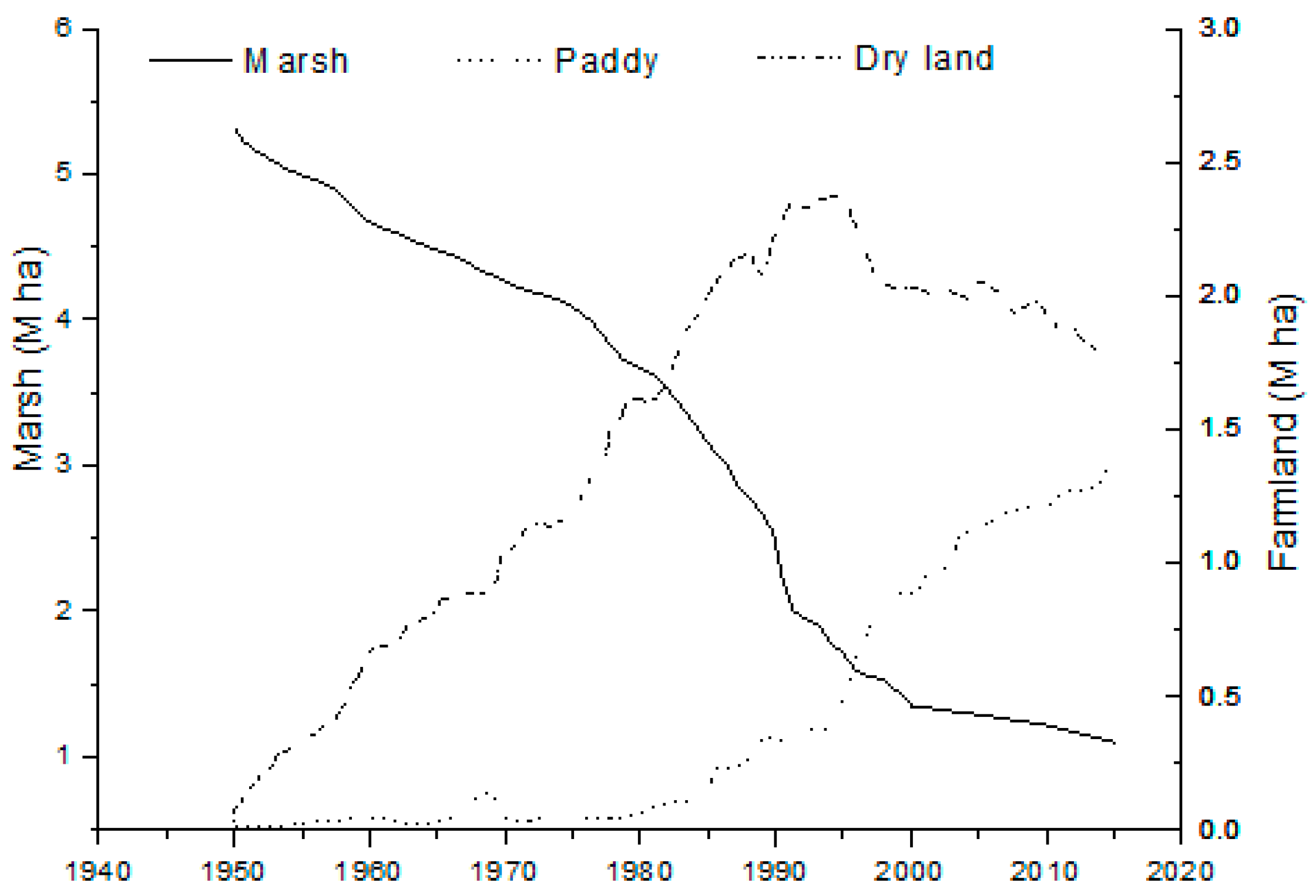
2.1. Study Area

From 1950 to 2015, cultivated land reclamation was the main land use change in Sanjiang Plain, northeast China, and was mainly represented by the transformation of dry lands to paddy fields. From 2000 to 2015, the land area of upland fields decreased continuously, whereas that of paddy fields increased consistently. The ratio of the two changed from 3.8:1 to 1.2:1 [24]. Figure 1 is the land use change map of Sanjiang Plain in the most recent 60 years. The data are from the Sanjiang Mire Wetland Experimental Station of the Chinese Academy of Sciences. Given this transformation, most areas of Sanjiang Plain has become mainly paddy fields. The study area is in the Sanjiang Mire Wetland Experimental Station of the Chinese Academy of Sciences, which belongs to the central part of the wetland agricultural ecological zone of Sanjiang Plain in northeast China. The region has a temperate semi-humid continental climate, with a total precipitation of approximately 600 mm and an average annual temperature of 1.9 °C. Regarding climate, the temperature in this region rises fast in spring and drops sharply in autumn. The land here is fertile, and the soil types are mainly black soil, white clay, swamp soil, and meadow soil. At present, the experimental station has 105 ha of field sites, mainly including swampy wetlands and marshy meadows. Seven hectares are upland experimental fields, and 6.6 ha are paddy field experimental fields. A microclimate observation system, an eddy covariance system, and other field observation facilities are also present here.

2.2. Methods

In this work, the land use change of uplands and paddy fields in Sanjiang Plain was studied using comparative analysis. According to the principal research line of “field observation–rule interpretation–model simulation”, this study explored the variation characteristics of surface water heat transport under the influence of land use change and revealed the variation status of surface water heat flux under different land use types. Finally, the variation trend of soil water and heat flux of varying land use types under future climate change was studied through model simulations.

2.2.1. Field Observation Method

The data in our study were the daily monitoring data in the Sanjiang Mire Wetland Experimental Station of the Chinese Academy of Sciences. Dry field and paddy field observations of the same facility were selected as the study samples, and the monitored period was May 2016 to May 2017. An eddy covariance system and a microclimate observation system were established in the study area to monitor soil water content, soil temperature, and soil water heat flux. The open-path eddy covariance system comprises an ultrasonic anemometer (Windmaster Pro, Gill, Lymington, UK), CO₂/H₂O analyzer (LI-7500A, LI-COR, Lincoln, NE, USA), CH₄ analyzer (LI-7700, LI-COR, Lincoln, NE, USA), temperature and humidity analyzer (HMP155, Vaisala, Vantaa, Finland), and data recording module (LI-7550, LI-COR, Lincoln, NE, USA). A microclimate observation system (CR1000, Campbell Scientific, Edmonton, AB, Canada) was used to observe the microclimate change near the ground and to study the effects of different meteorological factors on the surface water heat flux of varying land use modes. A soil temperature sensor observed the values of soil temperature and water content at different depths. Concurrently, the soil water content was measured using regular sampling to correct the sensor error and observation of the change law of soil water and heat transfer. The data for the entire year were divided into growing season (mid-May to mid-October) and freeze–thaw season (mid-October to mid-May of the following year) according to plant growth and air temperature. In the growing season, the indexes of plant height, leaf width, leaf surface area index, root depth, and aboveground dry biomass were measured in the paddy and upland fields. During the freezing–thawing season, the indexes of the cover thickness of the frozen soil in the samples were tested, and the results were used to correct the model parameters.

2.2.2. Model

The Simultaneous Heat and Water (SHAW) model was established by Flerchinger and Saxton of the USDA Northwest Watershed Research Center and is used to simulate the transport and exchange of water heat and solute flux during soil freezing and melting [25,26]. This model is effective and studies snowmelt and soil freezing and thawing in detail. The upper boundary of the system includes meteorological conditions at 2 m near the surface, whereas the lower limit is determined by soil conditions. The one-dimensional vertical profile consists of the snow layer, residue layer, and soil surface to the deep designated boundary (the depth can reach 4 m). The SHAW model can successfully simulate the hydrothermal motion of soil in the freezing–thawing zone [27,28].

The operation of the model requires a large amount of data including parameters of the study area, meteorological driving, soil hydraulic characteristics, and vegetation character. The simulated step size adopted in this work was a day, and the meteorological driving factor inputs were all daily data corresponding to the year and Julian date inputs. Data from sample plots in the Sanjiang Mire Wetland Experimental Station were used for the model simulation; the elevation was 56 m above sea level, the latitude was 47°35', and slope was 0. The vegetation of the sample plot was a single crop, and the planting of soybean in dry fields and rice in paddy fields consumed one year and one season. The root depth of vegetation was 60 cm, and indicators such as plant height, leaf width, leaf surface area index, and aboveground biological dry weight were measured in detail to address the demand of the model driving parameters. The hydraulic characteristics of soil varied considerably according to farmland use mode, and a comparison of hydraulic trait parameters is shown in

Table 1. Hydraulic characteristic parameters of different land use modes.

Depth/cm		10	20	40	60	80	100	120	150
Bulk density	Dry land	1.23	1.26	1.43	1.44	1.32	1.3	1.32	1.32
	Paddy	1.23	1.26	1.43	1.44	1.32	1.3	1.32	1.32
Saturated water content	Dry land	0.513	0.513	0.5	0.5	0.5	0.5	0.5	0.5
	Paddy	0.513	0.513	0.5	0.5	0.5	0.5	0.5	0.5
Saturated conductivity (cm/h)	Dry land	1	1	1	1	0.68	0.6	0.37	0.37
	Paddy	1	1	1	1	0.68	0.6	0.37	0.37

.

2.2.3. Simulation Accuracy Analysis

For a thorough analysis and evaluation of the simulation effect of the model, the estimation accuracy of model simulation was assessed using simulation efficiency (ME) [29], standard deviation (RMSE), average deviation (MBE), and average absolute error (RMAE).

$$\mathrm{ME}=1-\frac{{{\displaystyle \sum }}_{\mathrm{i}=1}^{\mathrm{N}}{\left({\mathrm{M}}_{\mathrm{i}}-{\mathrm{E}}_{\mathrm{i}}\right)}^2}{{{\displaystyle \sum }}_{\mathrm{i}=1}^{\mathrm{N}}（{\mathrm{M}}_{\mathrm{i}}-{\overline{\mathrm{M}}}_{\mathrm{i}}{）}^2}$$

(1)

$$\mathrm{RMSE}=\sqrt{\frac{1}{\mathrm{N}}{\displaystyle \sum }_{\mathrm{i}=1}^{\mathrm{N}}{\left({\mathrm{M}}_{\mathrm{i}}-{\mathrm{E}}_{\mathrm{i}}\right)}^2}$$

(2)

$$\mathrm{MBE}=\frac{1}{\mathrm{N}}{\displaystyle \sum }_{\mathrm{i}=1}^{\mathrm{N}}\left({\mathrm{M}}_{\mathrm{i}}-{\mathrm{E}}_{\mathrm{i}}\right)$$

(3)

$$\mathrm{RMAE}=\frac{\frac{1}{\mathrm{N}}{{\displaystyle \sum }}_{\mathrm{i}=1}^{\mathrm{N}}\left|\left({\mathrm{M}}_{\mathrm{i}}-{\mathrm{E}}_{\mathrm{i}}\right)\right|}{\frac{1}{\mathrm{N}}{{\displaystyle \sum }}_{\mathrm{i}=1}^{\mathrm{N}}{\mathrm{M}}_{\mathrm{i}}}\times 100\%$$

(4)

where M_i is the measured value; E_i is the model simulation value; ${\overline{\mathrm{M}}}_{\mathrm{i}}$ is the average of the measured values; and N is the number of observations. The closer the simulation efficiency is to 1, the smaller the standard deviation, and the better the model simulation effect. The more the average deviation and relative absolute error decreases, the closer the simulated value is to the observed value.

We validated the Simultaneous Heat and Water (SHAW) model simulation using data from May to July 2015 (

Table 2. Verification results of the model.

Depth/cm		Upland				Paddy
		ME/%	RMSE	MBE	RMAE	ME/%	RMSE	MBE	RMAE
Temperature	0	95.1	1.01	0.48	0.05	83.3	1.98	1.48	0.09
	5	96.3	0.83	0.59	0.04	88.4	1.55	0.93	0.08
	10	99.5	0.26	−0.05	0.01	90.5	1.37	0.63	0.08
	15	97.6	0.63	−0.11	0.04	91.6	1.27	0.43	0.07
	20	98.2	0.52	−0.15	0.04	90.4	1.31	−0.03	0.07
	40	98.6	0.43	−0.19	0.03	91.8	1.19	0.11	0.08
	60	95.5	0.73	−0.47	0.06	99.6	0.31	0.17	0.02
	100	96.9	0.56	0.47	0.06	99.8	0.20	0.19	0.02
Moisture	0	94.8	0.010	0.004	0.02	82.6	0.020	−0.003	0.029
	5	80.5	0.014	0.004	0.02	85.9	0.016	0.001	0.024
	10	82.1	0.016	0.009	0.04	76.8	0.013	0.002	0.020
	15	98.1	0.003	0.002	0.01	93.2	0.006	0.001	0.009
	20	96.3	0.002	0.004	0.04	86.4	0.009	−0.002	0.007
	40	94.9	0.002	0.001	0.03	86.6	0.01	0.001	0.018
	60	85.6	0.004	−0.001	0.01	84.4	0.01	−0.001	0.026
	100	97.9	0.001	0.001	0.07	86.8	0.01	−0.003	0.023

). It was verified that the simulation efficiency (ME) of soil temperature was more than 83%, mostly above 90%, indicating that the model could better simulate the change of soil temperature in the study area; the simulation efficiency (ME) of soil water content was higher than the minimum value of 76.8%, and the standard deviation (RMSE) was small, which can be a good simulation to reflect the soil moisture changes in the study area.

3. Results and Discussion

3.1. Variation Law of Soil Temperature and Humidity in Different Land Use Modes

The Sanjiang Plain is in a seasonally frozen soil area in China. The freezing–thawing cycle of soil results in complex changes in the water and heat transport of the soil, and the variations in temperature and precipitation directly impact the water and heat transport of the soil in shallow layers. Figure 2 shows that the trend of annual precipitation and temperature changes is concentrated in May and September, with a daily precipitation peak of 40 mm and annual precipitation of approximately 600 mm. The annual average temperature was around 2 °C, with the highest temperatures occurring in July and August and the lowest one showing in January.

Air temperature is a main factor influencing surface water heat condition. Figure 3 shows that the soil temperature varies with the air temperature. The fluctuation range of upper soil temperature is large and tends to flatten with increasing depth. With regard to annual variation, the fluctuation range of soil temperature is smaller than that of air temperature. From mid-October to April of the following year, the soil temperature at 0 cm above the surface was evidently higher than the air temperature. During the freezing–thawing period, on the one hand, the surface snow cover affected the energy exchange between the soil surface and atmosphere; on the other hand, the low thermal conduction property of snow cover affected the change in soil temperature, thereby causing the soil temperature to be higher than the air temperature.

As illustrated in Figure 3, the variation characteristics of soil temperature in the paddy and upland fields were roughly the same. With regard to the variation range, the surface layer was directly affected by solar radiation, and the temperature fluctuation range of the shallow soil was large. With increasing depth, the soil temperature change tended to flatten.

The change in precipitation considerably affected the evolution of soil water content, presenting a positive correlation. The soil moisture content increased with an increase in rainfall. During the growing season, the effect of rainfall on the upland fields was more substantial than that on the paddy fields. Therefore, the fluctuation range of soil moisture content in the upland fields was considerably wider than that in the paddy fields. With an increase in depth, this fluctuation tended to become gentle. Figure 4 shows that precipitation in the growing season caused the surface water supply to be greater than evaporation, thereby resulting in the infiltration of surface water to the lower soil and a sudden increase of soil water content. When precipitation decreased, soil moisture content decreased slowly. After mid-October, the temperature drop caused the shallow soil to freeze, and the water flux at the interface of the shallow soil began to approach zero. As the depth increased, the freezing time of the soil continued to be delayed. After complete freezing, the water flux of the soil interface became 0. Under the action of the matrix potential gradient, the water in the frozen soil layer transferred to the vicinity of the freezing front, thus leading to the low water content of the soil in the shallow layer. As the temperature rises, the snow layer on the soil surface starts to melt. As the depth increases, the melting time is delayed. The difference between the surface layer and the deep layer is approximately 10–15 days.

3.2. Modeling Analysis

3.2.1. Modeling Simulation Accuracy Analysis

Table 3. Soil temperature simulation results of different land use modes.

Depth/cm	Dry Field Temperature				Paddy Temperature
	ME/%	RMSE	MBE	RMAE	ME/%	RMSE	MBE	RMAE
0	93	2.93	−1.02	0.42	96.8	1.96	0.75	0.23
5	99	1.07	0.25	0.12	97.8	1.54	0.66	0.18
10	99	1.02	−0.63	0.13	97.6	1.59	0.78	0.18
15	99	0.64	0.2	0.07	97.9	1.42	0.79	0.16
20	98	1.12	0.02	0.15	97.9	1.33	0.59	0.15
40	98	0.86	0.2	0.11	98.8	0.93	0.35	0.1
60	98	0.78	0.16	0.1	99	0.77	0.17	0.08
100	100	0.29	−0.01	0.03	99.6	0.45	0.07	0.04

, which shows the soil temperature simulation results of various land use modes, reveals that the simulation effect of each layer was greater than 92%. With the increased soil depth, the simulation accuracy of the model on the soil temperature was improved. The reason may be that the shallow soil is greatly influenced by the outside world, and some errors exist in the soil parameters. In the model simulation results, the surface value of the standard deviation was relatively large and gradually decreased with increasing depth, and the simulation effect gradually improved. The average difference and relative absolute error progressively reduced with the increase of depth, indicating that the simulated value was close to the observed value. The negative average deviation values at 0, 10, and 100 cm indicated that the simulated amount was larger than the perceived value, and the model slightly overestimated the temperature change of the layer. However, in general, the standard deviation was between 0.29 and −2.93, indicating that the error between the simulated value and the observed value was within the acceptable range; thus, the simulated result can reflect the actual observation.

Soil water experiences complex effects due to many influencing factors such as the phase change of soil water, soil temperature, surface vegetation, precipitation, and soil particle size. Therefore, the simulation efficiency of soil water is relatively lower than that of soil temperature. The standard deviation of the soil water simulation value and observed value was between 0.01 and 0.05, indicating that the simulation result was closer to the observed one (

Table 4. Statistical analysis of soil water simulation results of different land use modes.

Depth/cm	Dry Field Moisture				Depth/cm	Paddy Moisture
	ME/%	RMSE	MBE	RMAE		ME/%	RMSE	MBE	RMAE
0	82.2	0.05	0.007	0.15	0	80	0.05	−0.017	0.19
5	91.4	0.03	0.007	0.09	5	86.2	0.05	−0.013	0.16
10	87.6	0.03	0.005	0.1	10	90	0.04	0.018	0.1
15	78.7	0.03	−0.009	0.11	15	83.6	0.05	0.025	0.11
20	90.8	0.02	0.014	0.07	20	91.5	0.03	−0.017	0.11
40	90.6	0.02	0.001	0.06	40	90.8	0.03	−0.005	0.09
60	79	0.02	0.008	0.06	60	95	0.02	0.002	0.06
100	85.2	0.01	0.005	0.02	100	79.6	0.03	0.005	0.09

). The analysis results showed that the simulated and observed values of soil moisture were similar, and the SHAW model could well simulate the change in soil moisture throughout the year.

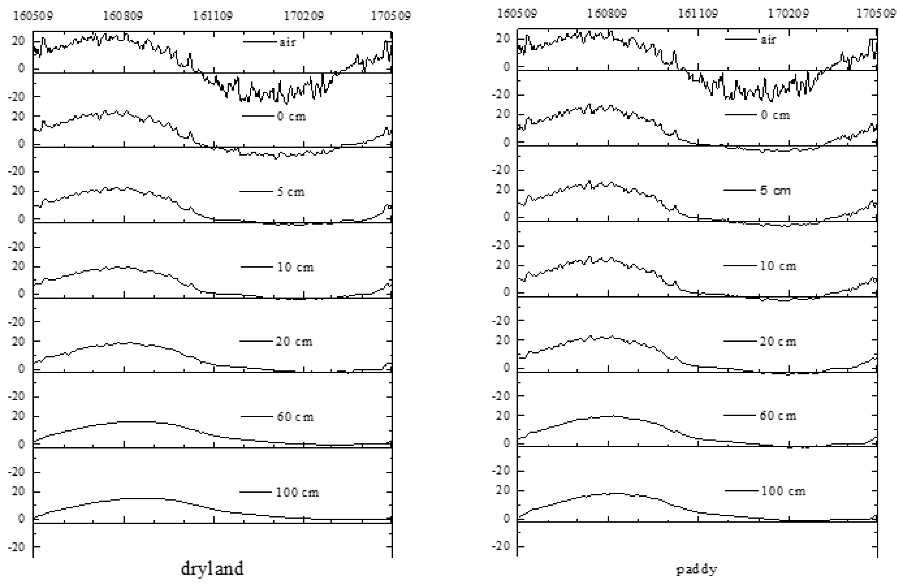
3.2.2. Soil Temperature

Soil profiles at 0, 60, and 100 cm depths were selected from two different land use modes in the upland and paddy fields for comparison. From the point of the year-round variations in soil temperature, the dry field surface average annual temperature was 5.9 °C, and the average annual temperatures at soil depths of 60 and 100 cm were 6.6 °C and 6.4 °C, respectively. In the paddy fields on the Earth’s surface, the average temperature was 7.6 °C, and the average annual temperatures at soil depths of 60 and 100 cm were 6.6 °C and 6.5 °C, respectively. Therefore, the soil temperature difference between the surface layers of the upland and paddy fields was evident, indicating that the surface temperature of paddy fields was larger than that of the upland fields and that the temperature difference decreased with increasing depth. The soil temperature began to increase in May, reached the maximum in July and August, started to decline in mid-October, and dropped to the minimum value in January and February. During the thawing period, the surface soil temperature rose rapidly, whereas the underlying soil temperature rose slowly due to the depth because the shallow soil was evidently affected by temperature change. The overall variation range of surface soil temperature was broad, and the variation tended to become gentle as the depth increased. As shown by the fluctuation of the soil temperature curve in Figure 5 and Figure 6, the daily temperature fluctuation of the soil surface due to many external factors was intense, but gradually disappeared with increasing depth [30]. During the conversion from uplands to paddy fields, the surface soil temperature increased. As the depth increased, the soil temperature in the upland and paddy fields tended to become identical.

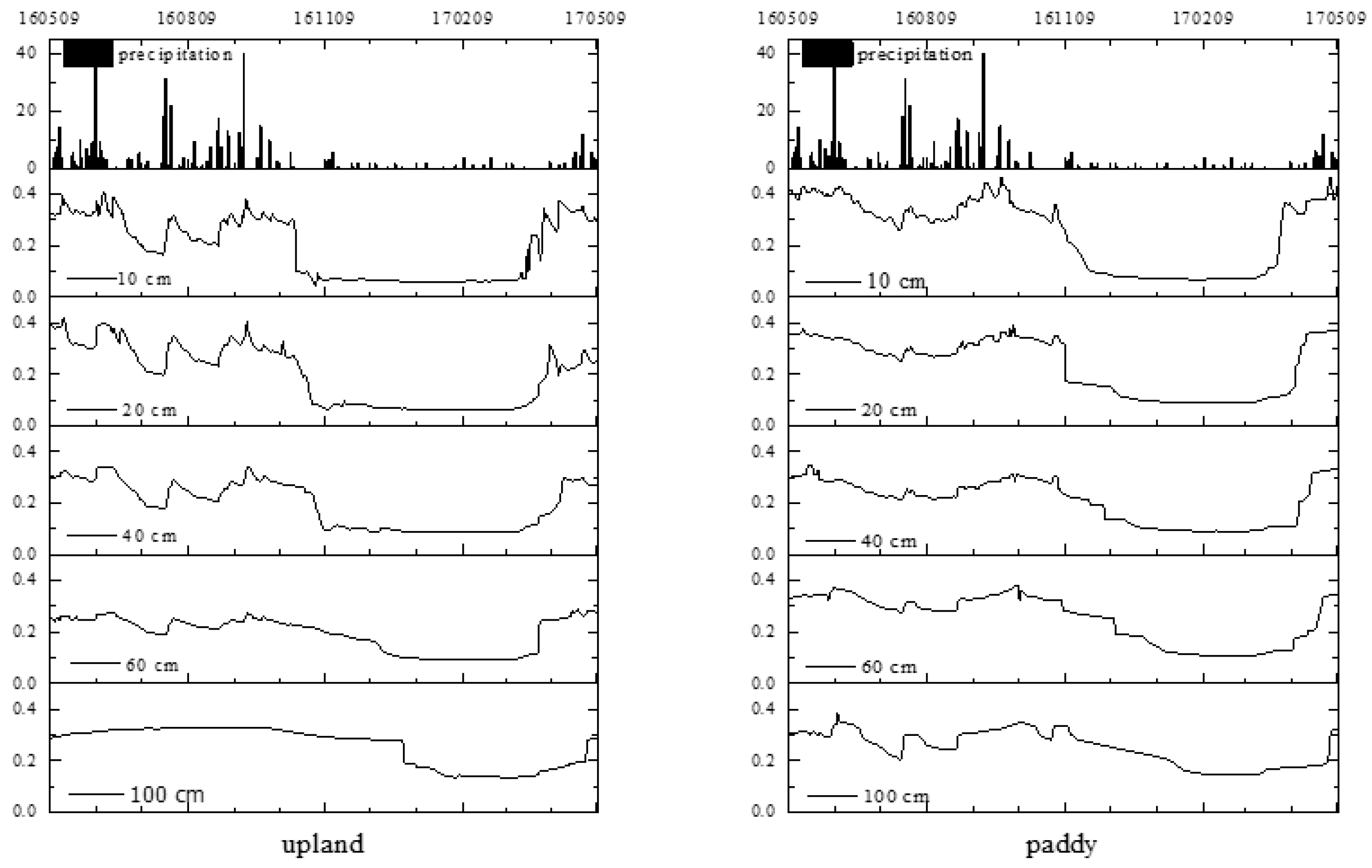
3.2.3. Soil Water Content

The upper, middle, and lower layers of the soil profiles with different land use patterns were selected for analysis and comparison. The variation trends of the simulated and observed values were consistent, and the simulation effect during the freeze–thaw period was slightly enhanced. The simulation results in Figure 7 and Figure 8 were close to the observation results. The first half of Figure 7 shows the fluctuation of soil water content in the growing season, and this change was quite intense. After the beginning of the freezing–thawing period, the water flux at the interface between the soil sections became zero. Thus, the water content of the surface soil remained at a stable state for a long time. During the ablation period, the frozen soil melts, and the snow cover melts on the ground, thereby leading to a rapid increase in soil moisture content. The soil water content is affected by factors such as atmospheric precipitation and surface vegetation, and the curve is volatile, unlike the smooth curve of the soil temperature simulation. The fluctuation range of the surface water content of the upland fields was larger than that of the paddy fields. The annual average of the soil water content of the upland fields at 10 cm depth was 0.21, and that of the paddy fields was 0.26. With an increase in depth, the annual average water content in the upland fields became 0.28. During the freezing–thawing period, the water content in the shallow soil decreased rapidly. With the increased soil depth, the decrease rate of the soil moisture content slowed. Consequently, the annual average soil moisture content increased during the conversion from upland to paddy fields, and the soil moisture content difference decreased with increasing depth.

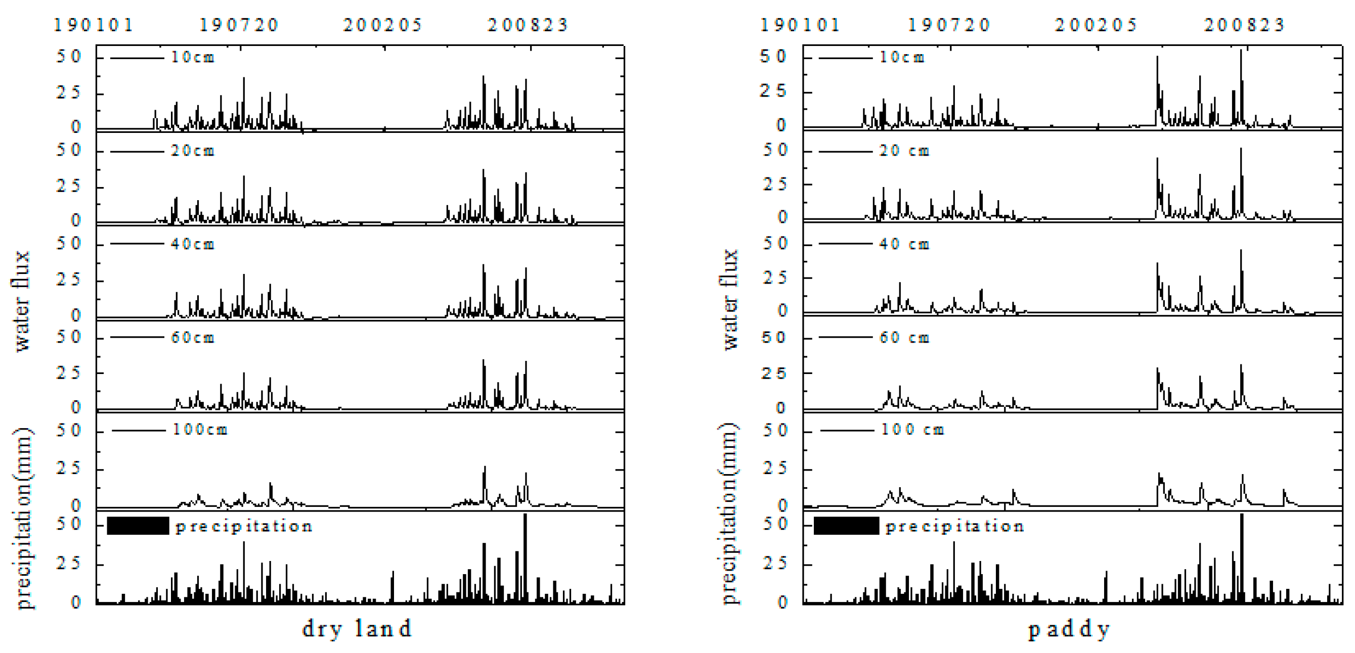
3.2.4. Soil Water and Heat Flux

Figure 9 shows the amount of the interannual variation of soil water infiltration. The total annual precipitation, annual infiltration amount in the upland surface, annual evapotranspiration, and surface water flux were 531.8, 363.2, 373.8, and −10.6 mm, respectively. For the paddy fields, the annual surface infiltration capacity, annual evapotranspiration, and surface water flux were 370.4, 375.6, and −5.2 mm, respectively. The annual variation of surface water flux in the upland fields was relatively small, and the surface water flux substantially differed at the growth season stage (Figure 10). The precipitation in the growing season was 446.9 mm, among which the surface infiltration amount in the upland fields, evapotranspiration volume, and surface water flux were 372.2, 267.7, and 104.5 mm, respectively. For the paddy fields, the surface infiltration capacity, evapotranspiration, and surface water flux were 108.7, 353.1, and −244.4 mm, respectively. Therefore, the surface water flux values of the upland and paddy fields substantially differed in the growing season. The surface infiltration amount in the upland fields was higher than that of the paddy fields, accounting for about 80% of precipitation. However, the evapotranspiration amount of the paddy fields was much higher than that of the upland fields, indicating that the evapotranspiration amount of the upland fields during the growing season takes about 60% of precipitation, and about 80% in the paddy field (Figure 11). The soil depth required for farmland plant growth is one meter. Therefore, the soil water flux at the bottom of 1 m in the upland and paddy field was analyzed. The annual infiltration at 1 m depth in the upland field was 230.8 mm, and the annual penetration of 1 m depth in the paddy field was 140.7 mm. The precipitation of the growing season was 446.9 mm, the infiltration at 1 m depth in the upland fields was 231.5 mm, and the infiltration at 1 m depth in the paddy fields was 108.9 mm. Accordingly, the evapotranspiration and infiltration of various land use types are evidently different. Figure 9 shows that the infiltration amount in the upland fields was much more evident than that of the paddy fields, and the surface water flux changed mainly in the growing season. In October, the surface of the soil began to freeze, and the water flux at the surface interface was 0. Evapotranspiration decreased rapidly, and the water potential of the frozen surface soil diminished. Consequently, the moisture in the unfrozen substratum transferred to the frozen area, and the water flux in the upward direction increased. Therefore, the negative water flux at the depth of 10 cm increased. Thus, the soil infiltration amount in the upland fields in the growing season was greater than the interannual soil infiltration amount. In April, as the temperature increased, the surface soil began to melt, the soil water content of the upper was high, and the soil water potential of the upper soil was large. Therefore, water was transported downward, resulting in a rapid increase in the forward water flux. With the rise of soil depth, soil water flux gradually decreased, so the water flux in each layer of the upland fields was greater than that in the paddy fields, and the depth of 100 cm was obvious.

Soil heat flux, which is an integral part of surface water and heat transport, shows the heat exchange between surface and deep soil. The change in soil heat flux varies with solar radiation intensity. Characteristics of soil heat flux variation in different land use types are similar. When the net radiation reaches the maximum, the soil heat flux also reaches the maximum, indicating the much higher soil heat flux in the paddy fields than in the upland fields (Figure 12). The maximum and minimum heat flux values were 52 and −40.8 w/m², respectively, in the paddy fields, whereas the maximum and minimum heat flux values were 31.7 and −19.5 w/m², respectively, in the upland fields. From the beginning of spring in March and April, when temperatures gradually increase, the absorbing solar radiation of the ground surface increases, and the soil heat flux starts becoming a positive value. The absorbing solar radiation of ground surface is more and less from September. The soil heat flux decreases rapidly before the soil begins to freeze. The series of changes in soil heat flux indicates that soil begins to change from heat absorption to an exothermic process. Furthermore, the intensity of the soil heat release gradually increases. During the freezing process, soil heat is transported to the surface, and soil heat flux is negative. Conversely, soil heat is carried to the deep soil from the surface in the thawing process. The soil heat flux changes in various periods because of the soil water phase transformation. The surface water heat flux varies in different land use types. Furthermore, the infiltration at 1 m in the upland fields was more than that in the paddy fields. However, the paddy fields have higher evapotranspiration and heat flux than the upland fields during the growing season. As the land use type changes from upland to paddy fields, the surface water and heat transportation changes evidently, mainly including the decreasing infiltration at 1 m, the considerably increasing surface evapotranspiration in the growing season, and the incremental surface heat flux.

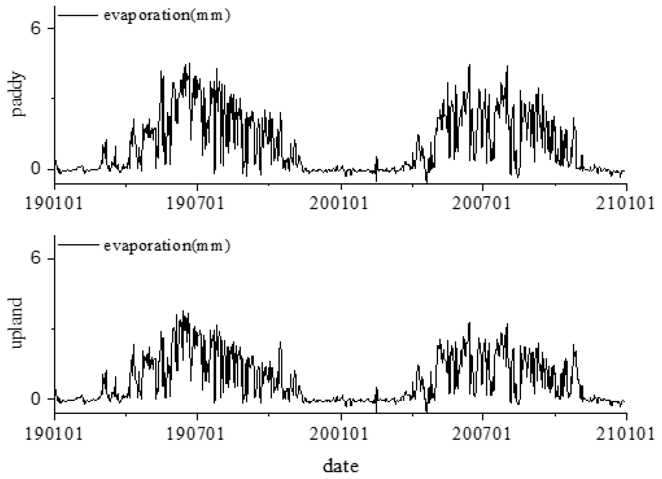
3.2.5. Changes in Soil Water and Heat Flux Under Future Climate Change Scenarios

On the basis of the meteorological forecast data of the IPCC AR5, a simulation study was conducted on the surface water heat flux of different land use types under the scenario of RCP4.5 emissions. The future climate change prediction data in this paper were obtained from the Earth System Grid Federation (ESGF) platform, and was predicted by National Oceanic and Atmospheric Administration (NOAA) agency simulation. The climate of the next two years was analyzed before the simulation (Figure 13). The analysis found that the average annual temperature decreases, and precipitation increases. The analysis of future climate prediction data showed that the annual average rainfall in the next two years is about 960 mm, among which the precipitation in the growth season is 660 mm. The average temperature in the next two years is 0.25 °C, about 2 °C lower than the average temperature in previous years. Figure 14 and Figure 15 show that the change of soil water flux varies with the change of precipitation. The soil water flux in the growing season is larger than that in the freeze–thaw season because the water flux at the soil interface is 0 in winter when the soil freezes. Figure 16 shows that in the future climate change scenario, the precipitation in the growing season is 660 mm, the evapotranspiration in the paddy field is greater than that in the upland field, the evapotranspiration in the upland is 267 mm, and the evapotranspiration in the paddy field is 369 mm, accounting for 40% and 55% of precipitation, respectively, which are lower than those in the present. Meanwhile, net radiation is a main factor affecting surface heat flux. In Figure 17, the surface heat flux varies with the net radiation value. The impact of future climate change will result in the occurrence of individual extraordinarily high and deficient surface water heat flux. However, the general trend of change is consistent with the current trend, which shows that the global climate model can predict climate change in northeast China well. However, the data simulated by the model showed a certain deviation; this can be attributed to the uncertainty of the climate model itself and to greenhouse gas emissions.

4. Conclusions

We analyzed the variation of surface water and heat transport of different land use, and a simulation analysis was conducted to investigate the change of water heat flux using observation data from the Sanjiang Mire Wetland Experimental Station. From the comparison of the two land use types, we can obtain the following conclusions.

Considerable differences in surface water heat transport and surface water flux were seen during the growing season in the upland and paddy fields. The precipitation in the growing season was 446.9 mm. The surface infiltration, evapotranspiration, and surface water fluxes were 372.2, 267.7, and 105.5 mm in the upland fields, respectively, and 108.7, 353.1, and −244.4 mm in the paddy fields, respectively. Evapotranspiration was about 60% of precipitation in the upland fields in the growing season, while it was approximately 80% in the paddy fields. The infiltration in the upland fields was much higher than that in the paddy fields. The change of surface water flux was mainly concentrated in the growing season. The transformation from upland to paddy fields led to changes in soil water and heat; the surface heat flux increased, the infiltration of surface soil water decreased, and surface evapotranspiration increased evidently during the growing season.

Soil temperature and moisture content in the upland and paddy fields was significantly different. The fluctuations of soil temperature were smaller than those of air temperature in both types. As upland changed into paddy fields, the surface soil temperature increased, and soil temperature changed gradually with depth. The annual mean soil water content values during precipitation at 10 cm depth in the upland and paddy fields were 0.21 and 0.26, respectively, and the annual mean water content values in both land use types at 100 cm depth became 0.28 with increased depth. Consequently, during the conversion of upland to paddy field, the average annual soil moisture content increased, and the soil moisture content difference decreased with increasing depth.

In the case of RCP4.5 emissions, the overall trend of soil water and heat changes was consistent with the current trend in the next two years (2019–2020). In the growing season, the evapotranspiration of the upland fields was lower than that of the paddy fields, and the proportion of upland and paddy fields in precipitation was 40% and 55%, respectively. The upland fields exceeded the paddy fields in the infiltration capacity of 1 m. However, the proportion of evapotranspiration to precipitation decreased when compared with the present.

References

1. Jiang, Y.; Wu, H. Simulation capabilities of 20 CMIP5 models for annual mean air temperatures in Central Asia. Progress. Inquis. Mutat. Clim. 2013, 9, 110–116. [Google Scholar]
2. Reinman, S.L. Intergovernmental Panel on Climate Change (IPCC). Encycl. Energy Nat. Resour. Environ. Econ. 2013, 26, 48–56. [Google Scholar]
3. Park, H.; Kim, Y.; Kimball, J.S. Widespread permafrost vulnerability and soil active layer increases over the high northern latitudes inferred from satellite remote sensing and process model assessments. Remote Sens. Environ. 2016, 175, 349–358. [Google Scholar] [CrossRef]
4. Luo, D.; Wu, Q.; Jin, H.; Marchenko, S.S.; Lu, L.; Gao, S. Recent changes in the active layer thickness across the northern hemisphere. Environ. Earth Sci. 2016, 75, 555. [Google Scholar] [CrossRef]
5. Peng, X.; Mu, C. Changes of soil thermal and hydraulic regimes in the Heihe River Basin. Environ. Monit. Assess. 2017, 189, 483. [Google Scholar] [CrossRef] [PubMed]
6. Bense, V.F.; Kooi, H.; Ferguson, G.; Read, T. Permafrost degradation as a control on hydrogeological regime shifts in a warming climate. J. Geophys. Res. Earth Surf. 2012, 117. [Google Scholar] [CrossRef] [Green Version]
7. Cheng, G.; Jin, H. Permafrost and groundwater on the Qinghai-Tibet Plateau and in northeast China. Hydrogeol. J. 2013, 21, 5–23. [Google Scholar] [CrossRef]
8. Ford, T.W.; Frauenfeld, O.W. Surface-atmosphere moisture interactions in the frozen ground regions of Eurasia. Sci. Rep. 2016, 6, 19163. [Google Scholar] [CrossRef]
9. Li, S.; Lai, Y.; Pei, W.; Zhang, S.; Zhong, H. Moisture–temperature changes and freeze–thaw hazards on a canal in seasonally frozen regions. Nat. Hazards 2014, 72, 287–308. [Google Scholar] [CrossRef]
10. Weiqiang, L.; Lei, Y.; Zhang, X.; Tian, K. Study of water and salt migration in soil under concrete mulch during freezing/thawing period. J. Glaciol. Geocryol. 2001, 3. [Google Scholar]
11. Zheng, X.; Fan, G. Influence of moisture content on infiltration characteristics in seasonal frozen and thawed soils. Trans. CSAE 2000, 16, 52–55. [Google Scholar]
12. Qiang, F.; Renije, H.; Zilong, W.; Tianxiao, L.; Xianghao, W. Soil thermal regime under snow cover and its response to Meteorological factor. Trans. Chin. Soc. Agric. Mach 2015, 46, 154–161. [Google Scholar]
13. Rui, J.; Xin, L. Improving the estimation of hydrothermal state variables in the active layer of frozen ground by assimilating in situ observations and SSM/I data. Sci. China 2009, 52, 1732–1745. [Google Scholar]
14. Qiang, F.; Renije, H.; Tianxiao, L.; Ziao, M.; Li, P. Soil moisture-heat transfer and its action mechanism of freezing and thawing soil. Trans. Chin. Soc. Agric. Mach. 2016, 47, 99–110. [Google Scholar]
15. Hirsch, A.L.; Guillod, B.P.; Seneviratne, S.I.; Beyerle, U.; Boysen, L.R.; Brovkin, V.; Davin, E.L.; Doelman, J.C.; Kim, H.; Mitchell, D.M.; et al. Biogeophysical impacts of land-use change on climate extremes in low-emission scenarios: Results from HAPPI-land. Earths Future 2018, 6, 396–409. [Google Scholar] [CrossRef] [PubMed]
16. Zhai Jun, S.Q.; Liu, J. Impact analysis of climate change from land use/cover change in inner Mongolia Plateau. J. Nat. Resour. 2014, 29, 967–978. [Google Scholar]
17. Song, K.; Liu, D.; Wang, Z.; Zhang, B.; Jin, C.; Li, F.; Liu, H. Land use change in Sanjiang Plain and its driving forces analysis since 1954. Acta Geogr. Sin. 2008, 63, 93–104. [Google Scholar]
18. Zhang, K. Impacts of Wetland Sucession on Soil Freezing and Thawing Process and Heat Exchange in Sanjiang Plain; University of Chinese Academy of Sciences: Huairou, China, 2011. [Google Scholar]
19. Lian, J.; Wang, J.; Zeng, H. Impacts of dramatic land use change on the near-surface air temperature in Shenzhen. Acta Sci. Nat. Univ. Pekin. 2017, 53, 692–700. [Google Scholar]
20. Ding, Q. Assessing the Impact of Land Use/Cover Change on Water and Heat Fluxes—A Case Applied GIS Study of Jiangxi Province; Shandong Normal University: Jinan, China, 2013. [Google Scholar]
21. Song, C.; Yan, B.; Wang, Y.; Zhao, Z.; Lou, Y. Effect of mires reclamation on soil moisture, temperature and characters. J. Soil Water Conserv. 2003, 6, 144–147. [Google Scholar]
22. Song, C.C.; Wang, Y.Y.; Yan, B.X.; Lou, Y.J.; Zhao, Z.C. The changes of the soil hydrothermal condition and the dynamics of C, N after the Mire Tillage. Environ. Sci. 2004, 25, 150–154. [Google Scholar]
23. Song, C.; Wang, Y.; Yan, B.; Zhang, J.; Lou, Y. Variation of soil temperature before and after cultivation of marsh and its effect on soil thermal regime. Chin. J. Appl. Ecol. 2005, 16, 88–92. [Google Scholar]
24. Zhang, L. Study on the Change of Cultivated Land Use under the Background of Climate Change in Sanjiang Plain. Master’s Thesis, Northeast Agricultural University, Harbin, China, 2017. [Google Scholar]
25. Flerchinger, G.N. Sensitivity of soil freezing simulated by the SHAW model. Trans. ASAE 1991, 34, 2381–2389. [Google Scholar] [CrossRef]
26. Flerchinger, G.N.; Saxton, K.E. Simultaneous heat and water model of a freezing snow-residue-soil System I. Theory and development. Trans. ASAE 1989, 32, 565–571. [Google Scholar] [CrossRef]
27. Flerchinger, G.N.; Kustas, W.P.; Weltz, M.A. Simulating surface energy fluxes and radiometric surface temperatures for two arid vegetation communities using the SHAW model. J. Appl. Meteorol. 1998, 37, 449–460. [Google Scholar] [CrossRef]
28. Link, T.E.; Unsworth, M.H.; Marks, D.G.; Flerchinger, G.N. Simulation of water and energy fluxes in an old growth seasonal temperate rainforest using the simultaneous heat and water (SHAW) model. J. Hydrometeorol. 2004, 5, 443–457. [Google Scholar] [CrossRef]
29. Nash, J.E.; Sutcliffe, J.V. River flow forecasting through conceptual models part I—A discussion of principles. J. Hydrol. 1970, 10, 282–290. [Google Scholar] [CrossRef]
30. Guo, D.; Yang, M. Simulation of soil temperature and moisture in seasonally frozen ground of Central Tibetan Plateau by SHAW model. Plateau Meteorol. 2010, 29, 1369–1377. [Google Scholar]
Figure 1. Land use change map of Sanjiang Plain in the most recent 60 years.
Sustainability 11 00157 g001
Figure 2. Annual change in temperature and precipitation.
Sustainability 11 00157 g002
Figure 3. Comparison of soil temperature and air temperature in upland and paddy fields.
Sustainability 11 00157 g003
Figure 4. Annual change of soil moisture content at different depths in upland and paddy fields.
Sustainability 11 00157 g004
Figure 5. Annual change of soil temperature in upland fields.
Sustainability 11 00157 g005
Figure 6. Annual variation of soil temperature in paddy fields.
Sustainability 11 00157 g006
Figure 7. Annual change of water content in upland soil.
Sustainability 11 00157 g007
Figure 8. Annual change of water content in paddy soil.
Sustainability 11 00157 g008
Figure 9. Annual variation of soil infiltration in upland and paddy fields.
Sustainability 11 00157 g009
Figure 10. Annual change of water flux in the soil profile at different depths in upland and paddy fields.
Sustainability 11 00157 g010
Figure 11. Annual variation of evapotranspiration of upland and paddy fields.
Sustainability 11 00157 g011
Figure 12. Annual variation of surface heat flux in upland and paddy fields.
Sustainability 11 00157 g012
Figure 13. Temperature and precipitation changes in the next two years.
Sustainability 11 00157 g013
Figure 14. Changes of soil water flux in the future.
Sustainability 11 00157 g014
Figure 15. Future tendency of infiltration of upland and paddy fields.
Sustainability 11 00157 g015
Figure 16. Future dry land and paddy evapotranspiration trends.
Sustainability 11 00157 g016
Figure 17. Changes of surface heat flux in the future.
Sustainability 11 00157 g017