Are Green Walls Better Options than Green Roofs for Mitigating PM₁₀ Pollution? CFD Simulations in Urban Street Canyons

Abstract

To examine the effect of green roofs (GRs) and green walls (GWs) on coarse particle (PM₁₀) dispersion in urban street canyons, a computational fluid dynamics (CFD) simulation was conducted with a Reynolds-averaged Navier-Stokes (RANS) model and a revised generalized drift flux model. Simulations were performed with different aspect ratios (H/W = 0.5, 1.0, and 2.0), greenery coverage areas (S = 300, 600, and 900 m²), and leaf area densities (LADs = 1.0, 3.5, 6.0 m²/m³). Results indicate that: (1) GRs and GWs all had the reduction ability of PM₁₀ at the pedestrian level; (2) Averaged concentrations of PM₁₀ in GWs and GRs varied little as LAD changed in H/W = 0.5 and 1.0. When H/W = 2.0, the aerodynamic effects of GRs increased since airflow was enhanced within street canyons, resulting in the increasing concentrations in GRs compared with non-greening scenarios; (3) Given equal greenery coverage area and aspect ratio, GWs are more effective in reducing street-canyon PM₁₀, and the averaged concentrations declined with increasing LADs and greenery coverage areas, especially the H/W; (4) At the pedestrian level, the reduction ratio of GRs is greater than that of GWs with the maximum value of 17.1% for H/W = 0.5. However, where H/W = 1.0 and 2.0, the concentrations within GWs are lower than GRs, with maximum reduction ratios of 29.3% and 43.8%, respectively.

1. Introduction

Global population data have shown that the urban residents numbered 4.0 billion in 2015, representing 54% of the total world population. Demographic models further predict that this proportion will exceed 60% (4.9 billion) in 2030 [1]. Rapid urbanization has turned cities into reinforced concrete forests accompanied by many environmental issues, such as rising urban temperature, prominent urban heat island effects, and continuously aggravated urban environmental pollution [2,3]. It has been well documented that urban greening plays a significant role in mitigating urban heat island effects and diluting particulate pollutants. Among the numerous forms of greening infrastructure, green roofs (GRs) and green walls (GWs) are preferred, especially for congested urban environments, because these two greening modes do not take up additional space. In addition, GRs and GWs have obvious positive effects on improving local air quality in the built environment [4,5,6].

Vegetation dilutes and reduces particulate pollutants through the influence of plant crowns on airflow fields and particulate pollutant dispersion [7,8]. Different vegetation types and planting patterns are the main factors affecting particulate dispersion [9,10,11]. Using a dry deposition model, Yang et al. indicated that GRs can reduce both gas contamination (O₃, NO₂, and SO₂) and concentration of suspended particulate pollutants (PM₁₀) [12]. Currie and Bass used the UFORE model to analyze retention effects of different vegetation patterns on air pollutants, reporting that dust-retaining effects of shrubs on GRs is greater than that of trees [13]. Moradpour et al. used NO-NO₂-O₃ photochemistry and energy-balance models to analyze the absorption effect of GRs on nitric oxides and ozone under different aspect ratios in street canyons and leaf area densities and found that GRs in deeper street canyons are more effective in improving air quality [14]. A field study of dust-retaining effects of GRs measured the CO₂ distributions surrounding roof greening but neglected the influence of vegetation on periphery airflow [15]. Results of Baik et al. indicated that improving air quality on adjacent roads is mainly due to GRs strengthening airflow fields near the ground in street canyon spaces [16].

Related research has been conducted on the dust-retaining effects of GWs. Pugh et al. used the CiTTy-street model to analyze pollutant absorption of street canyon greening reporting that vertical greening in street canyons can cut PM₁₀ by 60% [17]. Ottelé et al. compared the dust-retaining effects of vertical greening adjacent to roads and forests and indicated that small particulate pollutants are easily retained by GWs [18]. By incorporating the Large Eddy Simulation (LES) turbulence model into the Comprehensive Turbulent Aerosol Dynamics and Gas Chemistry (CTAG) model, Tong et al. compared the effects of six near-road vegetation barriers on particle concentrations on and near the road [19]. Measurements have also shown the ability of GWs to capture fine dust as a function of plant leaf shape and surface type (i.e., thick cuticular waxes on leaves epidermis) but unrelated to season or leaf age [20]. Field experiments have demonstrated that smaller leaves of living wall plants have greater capture capability for all PM size fractions [21]; and a rooftop farm had 7%–33% less PM concentration than at ground level [22]. Simulations and field studies have also analyzed the influence of GRs on the dispersion of air suspended particulate pollutants. Kessler stated that GWs may be a better option for mitigating street-canyon pollution than trees or GRs [23]. Moreover, a modeling and measurement study indicated that GWs are beneficial at near or far distances but worsen air quality above the pedestrian level [24]. The Guidance on Construction of London Garden City recommends that increasing urban GRs by 70% can reduce PM₁₀ concentrations by 0.5% [25]. However, little research has considered the interaction of urban forms and vegetation on particle deposition in urban street canyons [17,26].

Nevertheless, it is currently difficult to draw clear relationships among green infrastructure and particulate pollution on the basis of available research: whether GRs or GWs have better dust-retaining effects in urban street canyons. Moreover, few studies have conducted quantitative comparisons between GRs and GWs in improving air quality under controlled conditions (equal coverage area, identical vegetation type and identical plantation environment). To fulfill this gap, it is necessary to clarify the influence of green infrastructure in street canyons on particulate dispersion in different architectural spatial forms so as to quantitatively segregate the effects of GRs and GWs on particulate pollutant absorption.

Based on the RANS and revised generalized drift flux models, this study used the CFD code PHOENICS (Parabolic Hyperbolic Or Elliptic Numerical Integration Code Series) to evaluate the influence of GRs and GWs on airflow fields and PM₁₀ dispersion under different leaf area densities (LADs = 1.0, 3.5, and 6.0 m²/m³) with three levels of street canyon aspect ratios (H/W = 0.5, 1.0, and 2.0) and areas of greenery coverage (S₁ = 300, S₂ = 600, and S₃ = 900 m²) in street canyons. Additionally, a non-greening environment was also simulated to compare the results with that of vegetated conditions to quantify the overall reduction of PM₁₀ concentration by GRs and GWs.

2. Methodology

2.1. Flow and Dispersion Model

2.1.1. Model Description

A three-dimensional steady-state isothermal flow simulation model was used to reproduce and simulate airflow and dispersion in an idealized street canyon. CFD numerical simulation settings refer to the COST Action 732 standard, including choices of target variables, approximate equations, the geometrical representation of obstacles, the computational domain, boundary conditions, initial data, computational grid, numerical approximations, and iterative convergence criteria [27]. The Reynolds-averaged Navier-Stokes (RANS) model, which contains the k-ε Murakami-Mochida-Kondo (MMK) turbulence closure scheme, is adopted in the simulation. This model is modified based on the standard k-ε model. The Semi-Implicit Method for Pressure-Linked Equations (SIMPLE) algorithm with the Quadratic Upstream Interpolation for Convective Kinematics (QUICK) discretization scheme was applied to all governing equations except the concentration equation. The scaled iterative convergence criteria for all parameters were taken as 10⁻⁶. Simulations were processed using an i7 2.67 GHz processor (Intel, Santa Clara, CA, USA). The PHOENICS 2009 (CHAM, London, UK) program was used to determine the solution.

Vegetation is regarded as porous medium in the model, and its influence on airflow fields is measured by adding momentum source term, turbulent kinetic energy and turbulent dissipation rate in a relational computing grid of GRs and GWs. The continuity and momentum equations are expressed as follows:

Continuity equation:

$$\frac{\partial \left(u_i\right)}{\partial x_i}=0$$

(1)

where u_i is the spatial average velocity, and x_i is the spatial coordinate.

Momentum equation:

$$\frac{\partial \left(u_i\right)}{\partial t}+\left(u_j\right)\frac{\partial \left(u_i\right)}{\partial x_j}=-\frac{1}{\rho }\frac{\partial \left(P\right)}{\partial x_i}+\frac{\partial }{\partial x_j}\left({\nu }_{eff}\frac{\partial \left(u_i\right)}{\partial x_j}\right)+S_{Ui}$$

(2)

where P is the pressure (Pa), ρ is the air density (kg/m³), S_Ui is a drag term imposed by the vegetation, and v_eff is the effective viscosity (N s/m²) that is computed as:

$${\nu }_{eff}=\nu +{\nu }_t=\nu +c_{\mu }\frac{k^2}{\epsilon }$$

(3)

where k is the turbulent kinetic energy (Nm), ε is the dissipation rate (m/s), v_t is the turbulent kinetic viscosity (N s/m²), and c_μ is an empirical constant that set to 0.09 [28].

The drag force term, which is proportional to the leaf area density (LAD) and the plant drag coefficient, is expressed as:

$$S_{Ui}=-\rho C_d\alpha (z)\left|U\right|U_i$$

(4)

where ρ is ambient air density, C_d is the dimensionless drag coefficient, α(z) is the leaf area density at height z (m²/m³), |U| is the magnitude of the superficial velocity vector (m/s), and U_i is the superficial Cartesian velocity in the ith direction (m/s).

Vegetation density is characterized by the integral value of LAD. This integral value is determined by the leaf area index (LAI), which is defined as:

$$LAI={\displaystyle \underset{o}{\overset{h}{\int }}\alpha \left(z\right)}dz$$

(5)

where h is the average height of the canopy.

To simulate turbulence interactions between the plant canopy and airflow caused by leaves, the wake turbulence model, including additional source terms in the transport equations for k and ε, is used in canopy cells:

$$S_k=\rho C_d\alpha \left(z\right)\left({\beta }_p{\left|U\right|}^3-{\beta }_d\left|U\right|k\right)$$

(6)

$$S_{\epsilon }=\rho C_d\alpha \left(z\right)\left(C_{4\epsilon }{\beta }_p{\left|U\right|}^3\raisebox{1ex}{$\epsilon $}\!\left/ \!\raisebox{-1ex}{$k$}\right.-C_{5\epsilon }{\beta }_d\left|U\right|\epsilon \right)$$

(7)

where the constant β_p is the fraction of mean-flow kinetic energy converted to wake-generated k, and β_d is the fraction of k dissipated by short-circuiting of the Kolmogorov energy cascade. C_4ε and C_5ε are closure constants. β_p, β_d, C_4ε, and C_5ε are, respectively, set as 1.0, 3.0, 1.5, and 1.5 in this study [29,30,31].

A revised generalized drift flux model, modified from the Eulerian model, is used as an influence model of vegetation on pollutant dispersion. This model is a widely used Eulerian model, and treats particles as a continuum in particle conservation equations considering slippage between particles and flow (air) fields [32,33]. Due to the deposition action of plants on particles and effects of rain washing or wind, some particles will be re-diffused into air. Therefore, the deposition and resuspension effects of vegetation on particles are expressed by adding additional terms (S_sink and S_resuspension). In this way, the model can comprehensively and accurately reflect particle dispersion in a real urban environment. This model is expressed as:

$$\frac{\partial \left[\left(V_j+V_{g,j}\right)C\right]}{\partial x_j}=\frac{\partial }{\partial x_j}\left[{\epsilon }_p\frac{\partial C}{\partial x_j}\right]+S_c-S_{\sin k}+S_{resuspension}$$

(8)

The deposition effect of plant canopies, depending on LAD, deposition velocity, and ambient particle concentration, are described as:

S_sink = α(z) × V_d × C

(9)

Particulate resuspension is calculated as a volumetric source term, and described as:

S_resuspension = α(z) × V_r × C_sink

(10)

where V_j and V_g,j are the averaged fluid (air) velocity and the gravitational settling velocity of particles in j-th direction(m/s), respectively. C is the averaged concentration of particles (μg/m³), ε_p is the diffusion coefficient of the pollutant in the air (m²/s), S_c is the source term of pollutant (kg/(m^3▪s)), S_sink is the mass of particles absorbed per unit vegetation volume per unit time (μg/m³), S_resuspension is the particles resuspended from foliage per unit vegetation volume per unit time (μg/m³) [34], V_d is the particle deposition velocity on plant foliage (m/s), V_r is the particle resuspension velocity from plant foliage (m/s), α(z) is the leaf area density at the height z (m²/m³), and C_sink is the particle concentration deposited on plant foliage (μg/m³).

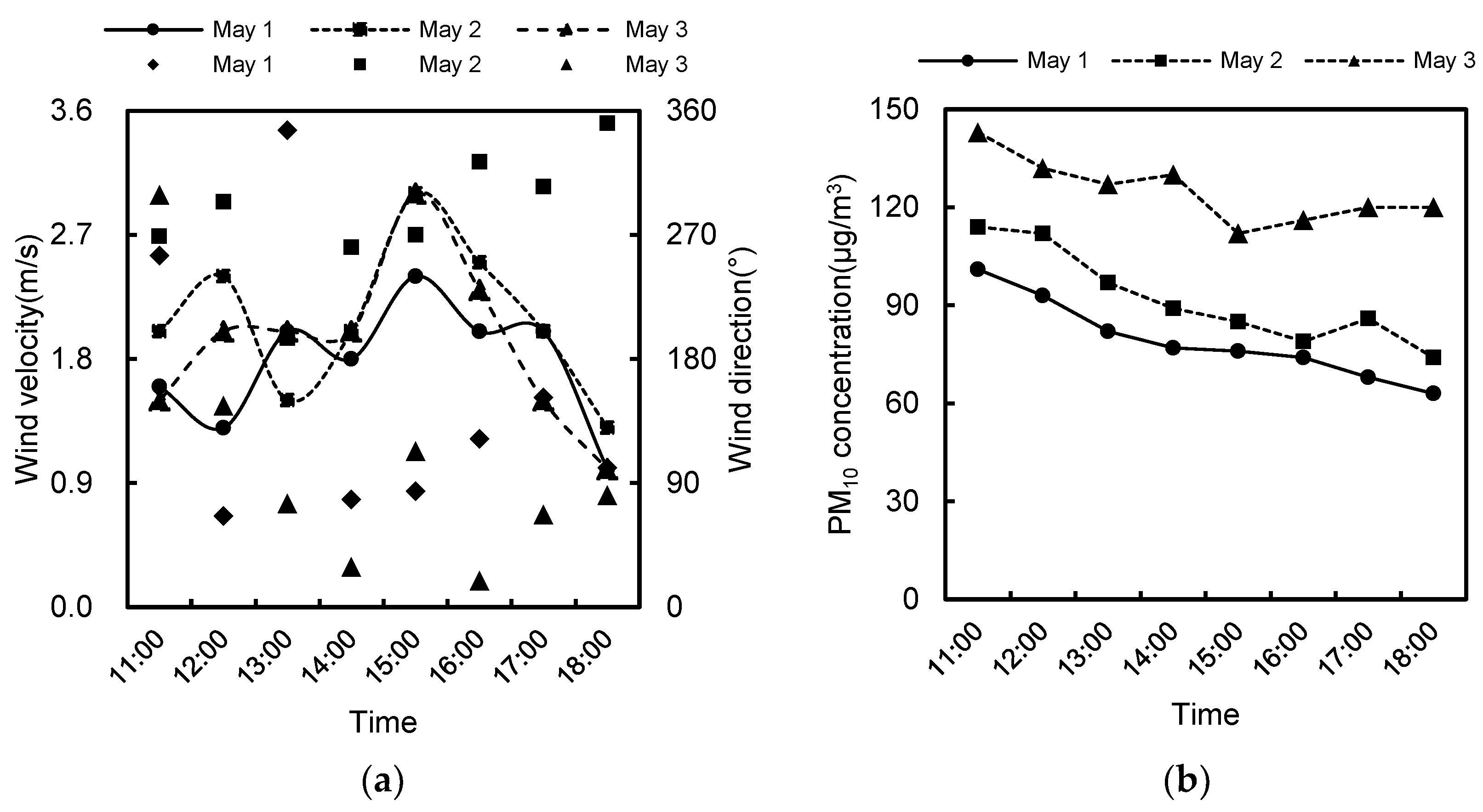
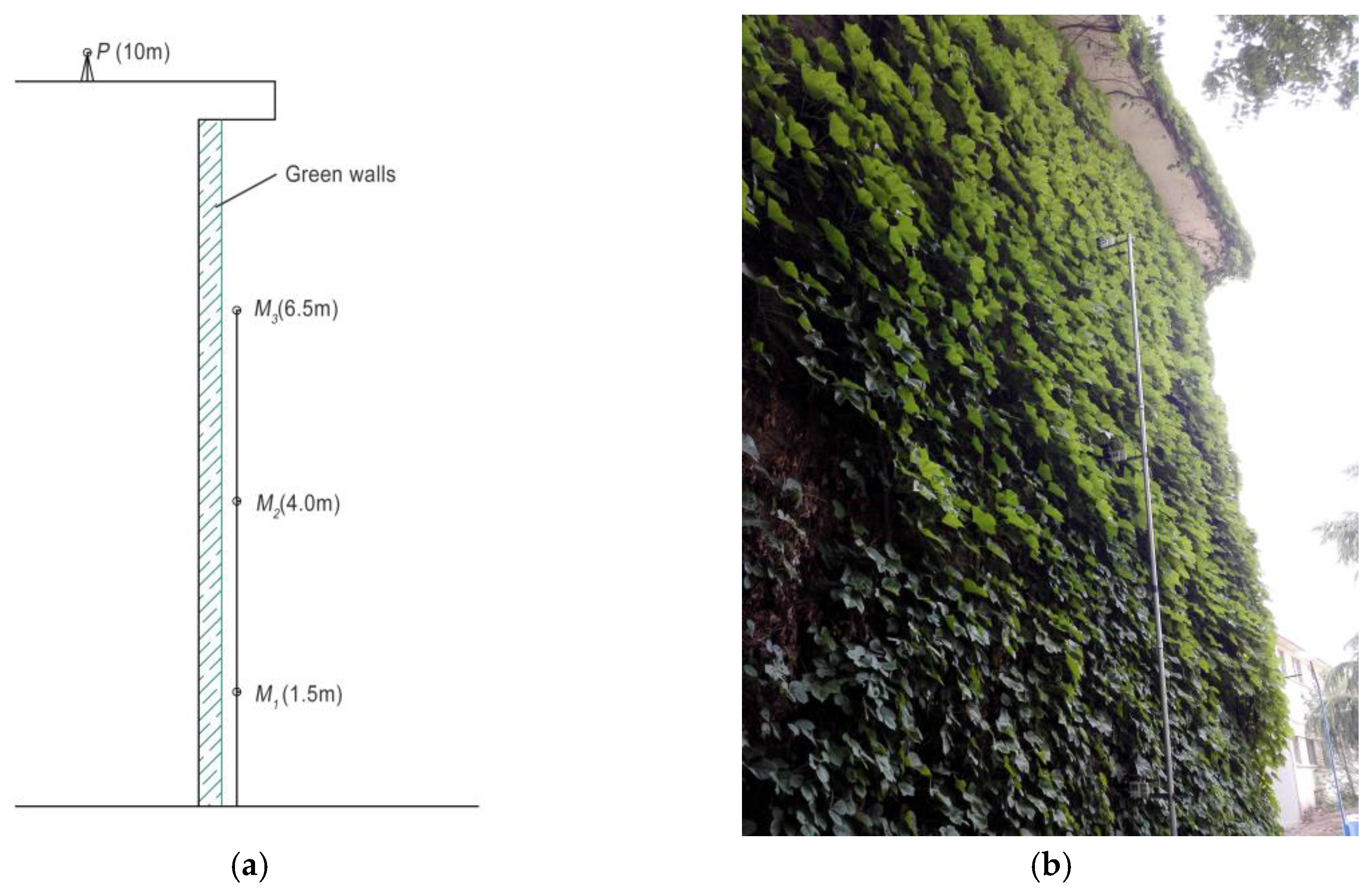
2.1.2. Model Validation

These models were validated by measuring in situ green walls in a Beijing residential district from 1 May to 3 May 2016. There, residential buildings have broad peripheries without influences from other buildings or high trees. The GWs are on western walls, comprised of Virginia Creeper (Parthenocissus vitacea), with a coverage ratio of 100%. The measurement period was from 11:00 to 18:00 at three measuring points (M₁, M₂, and M₃) set at 1.5, 4.0, and 6.5 m above the wall greening to monitor PM₁₀ concentrations at different heights (Figure 1). A measuring point (P) was set on the roof of the building (10 m) to monitor meteorological parameters including the incoming wind speed, wind direction using a Kestrel 5500 (Nielsen-Kellerman Inc., Boothwyn, PA, USA), and PM₁₀ concentrations using Metone 531S (METONE INSTRUMENTS, Inc., Grants Pass, OR, USA). These parameters were measured at five-minute intervals and averaged hourly. A LAI-2200C Plant Canopy Analyzer (LI-COR Inc., Lincoln, NE, USA) was used to test LAD determined by the total one-sided area of leaves per unit volume of Virginia creeper. The three dimensions of the building, length (L’ = 40 m), width (W’ = 15 m), height (H′ = 10 m), were also recorded.

The model was built according to site dimensions. Size of computational domain was set based on the recommendations [27,35]. The distance from the inlet to the windward building, from the downwind building to the outlet, and from the buildings to both boundaries were set to 5H′, 20H′, and 9H′, respectively. The height of the domain was 11H′. Three different grid sizes (coarse meshes: X_min = Y_min = Z_min = 0.10H′, fine meshes: X_min = Y_min = Z_min = 0.02H′, and finest meshes: X_min = Y_min = Z_min = 0.01H′) were set in the target area and the grid convergence index (GCI), calculated by the Equations (11)–(13), was applied to evaluate the grid independence. The GCIs were 2.97% for coarse and fine meshes, and 2.61% for fine and finest meshes (all less than 5%), indicating that the fine meshes were sufficient to conform to computational requirements [36].

$$GCI=F_s\frac{{\xi }_{rms}}{r^p-1}$$

(11)

$${\xi }_{rms}={\left(\frac{{\displaystyle {\sum }_{i=1}^n{\xi }_{i,u}^2}}{n}\right)}^{\frac{1}{2}}$$

(12)

$${\xi }_{i,u}=\frac{u_{i,coarse}-u_{i,fine}}{u_{i,fine}}$$

(13)

where F and p are empirical constants, and respectively defined as 3 and 2; r is the ratio of fine grid to coarse grid size, and u is the velocity magnitude (m/s).

Boundary condition settings refer to measured values at point P (Figure 2). The deposition velocity of Virginia Creeper was set as 0.64 cm/s [37,38]. Values obtained through simulation were compared with average measured data over three days. Comparisons between the measurement data at M₃ and M₁ and situation data at the same height indicated favorable correlations between simulation and field data (Figure 3, R² = 0.910 at M_3, and R² = 0.974 at M₁). Additionally, a set of acceptance criteria were selected to examine whether the data satisfy target values [39,40]. All metrics obtained were within the allowable ranges, indicating the models could suitably reproduce the actual environment of street canyon (

Table 1. Statistical analysis of model performance with the corresponding target values and a range of acceptance criteria.

Metrics	Target Value	Acceptance Criteria [39,40]	Reference Model Performance
			Upper Sampling	Lower Sampling
FB	0	−0.3 < FB < 0.3	−0.007	−0.047
NMSE	0	NMSE < 1.5	0.011	0.005
FAC2	1	0.5 < FAC2 < 2	1.007	1.048
MG	1	0.7 < MG < 1.3	0.954	0.944
VG	1	VG < 4	1.018	1.006
NAD	0	NAD < 0.3	0.042	0.031
R	1	0.8 < R	0.952	0.985

Note: FB—fractional bias; NMSE—normalized mean square error; FAC2—fraction within a factor of two of the observations; MG—geometric mean bias; VG—geometric variance, NAD—normalized absolute difference; and R—correlation coefficient.

). Additionally, the present authors compared this model with a wind tunnel experiment from a previous study that also showed that this model could accurately represent the actual street canyon environment [41].

2.2. Numerical Simulation

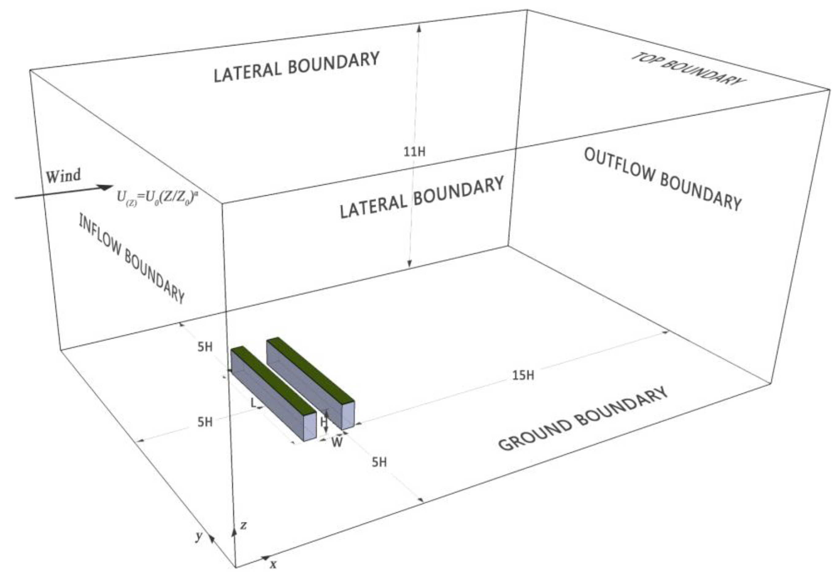
2.2.1. Numerical Model Setting

To investigate the effects of GRs and GWs on PM₁₀ concentration distributions in different street canyon configurations, street canyon aspect ratios (H/W) were set to 0.5, 1.0, and 2.0. Since the dust-retaining ratio of the building envelope was low, it was treated as a solid block without consideration of dust retention and wind penetration [41]. Herbaceous plants are generally used for GWs with a height of 0.1–0.5 m [42]. Herbs and shrubs were commonly used for roof greening with a height of 0.2–1.0 m [43,44]. To make research results comparable, it is assumed that herbs were planted for both GRs and GWs at the height of 0.3 m in the study. The greenery coverage areas were 300 m² (S₁), 600 m² (S₂), and 900 m² (S₃). The LAD of herbs ranges 1.0 to 6.0 m²/m³ according to available literature [45], thus, LADs were respectively adopted as 1.0, 3.5, and 6.0 in this research. Due to differences in morphological characteristics of plant leaves and ambient environments, the deposition velocities of most plants are within 0.01–10 cm/s [46,47]. V_d value as 0.64 cm/s in research of Nowak was used in this research [17,37,38]. This value is very commonly used and is suitable for our research as it is identical with deposition velocity of herbs predicated by Petroff and Zhang using a process-based model [48]. In all, fifty-four cases with three levels of aspect ratios, greenery coverage areas, and leaf area densities were built for this study (Figure 4).

2.2.2. Domain Size and Grid Independence Testing

This model is of an isolated street canyon with a north-south orientation, representing the most common forms in Beijing, China. The street is 18 m wide (W), and are set to 9, 18, and 36 m high (H) to create three levels of street canyon aspect ratios, i.e., shallow street canyon, symmetric street canyons, and deep street canyon. This corresponds to H/W = 0.5, 1.0, and 2.0 and simulates categorized airflow patterns, including isolated roughness flow, wake interference flow, and skimming flow in the street canyons [49]. The length of the street canyon is 100 m. Based on recent guidelines [27,35], the distance between the inlet boundary and the windward façade of the front building is 5H, and between the outlet boundary and leeward façade of back building is 15H. The distance between the symmetrical lateral boundary to the target area in 5H, and the distance from the ground boundary to top boundary is set as 11H (Figure 5).

A structural hexahedral mesh was used to ensure reasonable computing time. The target area within the street canyon consisted of the smallest cell dimension of the cells of X_min = Y_min = Z_min = 0.027H, while the grid expansion ratio was 1.2 outside the target area. Thus, the total cell number of the computational domain was approximately 6.2 million to ensure a higher resolution in the interested region. Grid independence was tested by the GCI [36]. The GCI value is 2.67% following the procedures implemented by Hefny and Ooka [50]. This result indicates that the given grid arrangement is adequate to distinguish simulations.

2.2.3. Boundary Conditions

Boundary conditions, including the inlet, outflow, top, ground, and lateral, are set to reproduce the atmospheric boundary layer. To represent wind transported and traffic-originated pollutant dispersions, two types of pollution sources were added: one though the inflow boundary, and another was added as line sources in intersections exceeded the street canyon by approximately 10% on each side [51]. Since the highest level of pollutant occurs from mid-November to December [52]. The averaged PM₁₀ concentration is 96 μg/m³ during this period [53]. Thus, this value was selected for the numerical simulations.

For the inlet boundary, a power law profile mean velocity was adopted and expressed as:

$$u\left(z\right)=u_0{\left(z/z_0\right)}^{\alpha }$$

(14)

where u(z) is the horizontal velocity at height z, u₀ is the horizontal velocity at the height of z₀. In this study, the averaged wind velocity during mid-November to December is 2.1 m/s with a westerly direction. In the model, u₀ = 2.1 m/s, z₀ = 10 m, and α = 0.25 [51].

The turbulent kinetic energy, k (m²/s²), and its dissipation rate, ε (m²/s³), are set as:

$$k=\frac{u_{\ast }^2}{\sqrt{C_{\mu }}}\left(1-\frac{z}{\delta }\right)$$

(15)

$$\epsilon =\frac{u_{\ast }^3}{kz}\left(1-\frac{z}{\delta }\right)$$

(16)

where u_* is the friction velocity, δ is the boundary layer depth, k is the von Kàrmàn constant, C_μ is a model constant, u_* = 0.52 m/s, k = 0.4, and C_μ = 0.09 [54].

A fixed pressure and zero gradients were specified for the outflow boundary. A fully rough wall function was implemented for the ground boundary. The constant horizontal velocity and turbulent kinetic energy that corresponds to the inflow profile were fixed to the top boundary, and the lateral planes were simulated as symmetric boundaries.

3. Results and Discussion

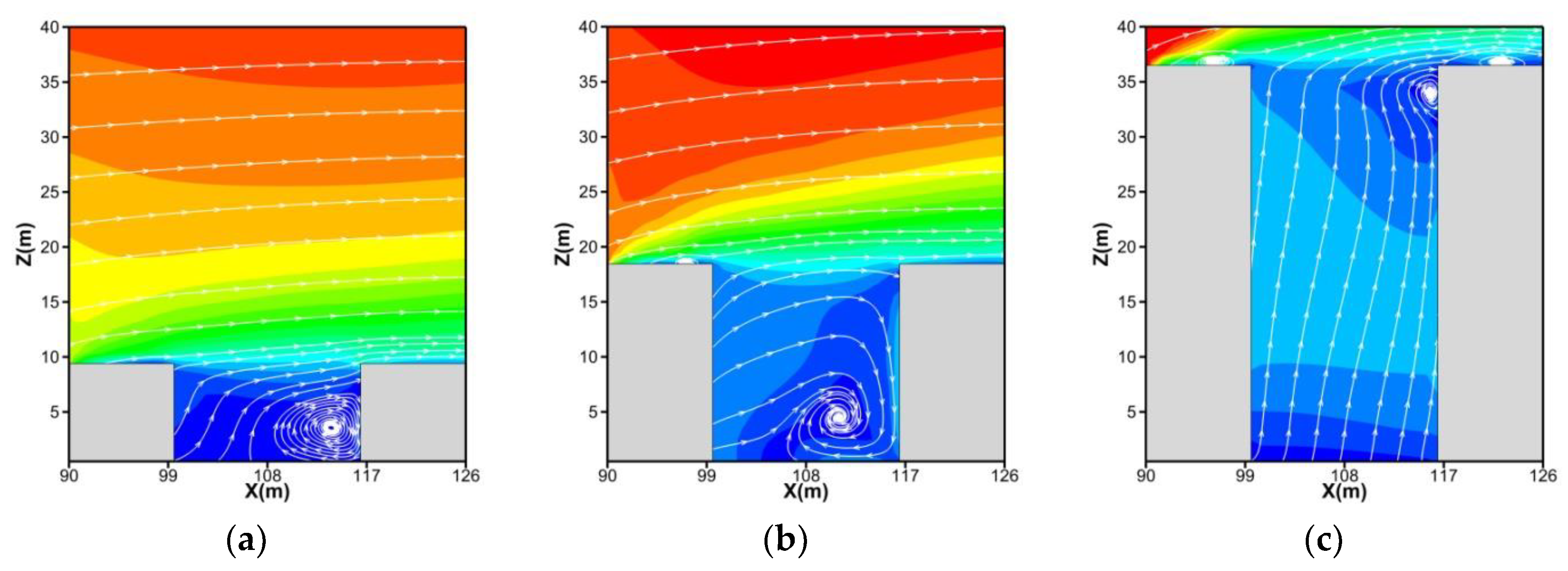
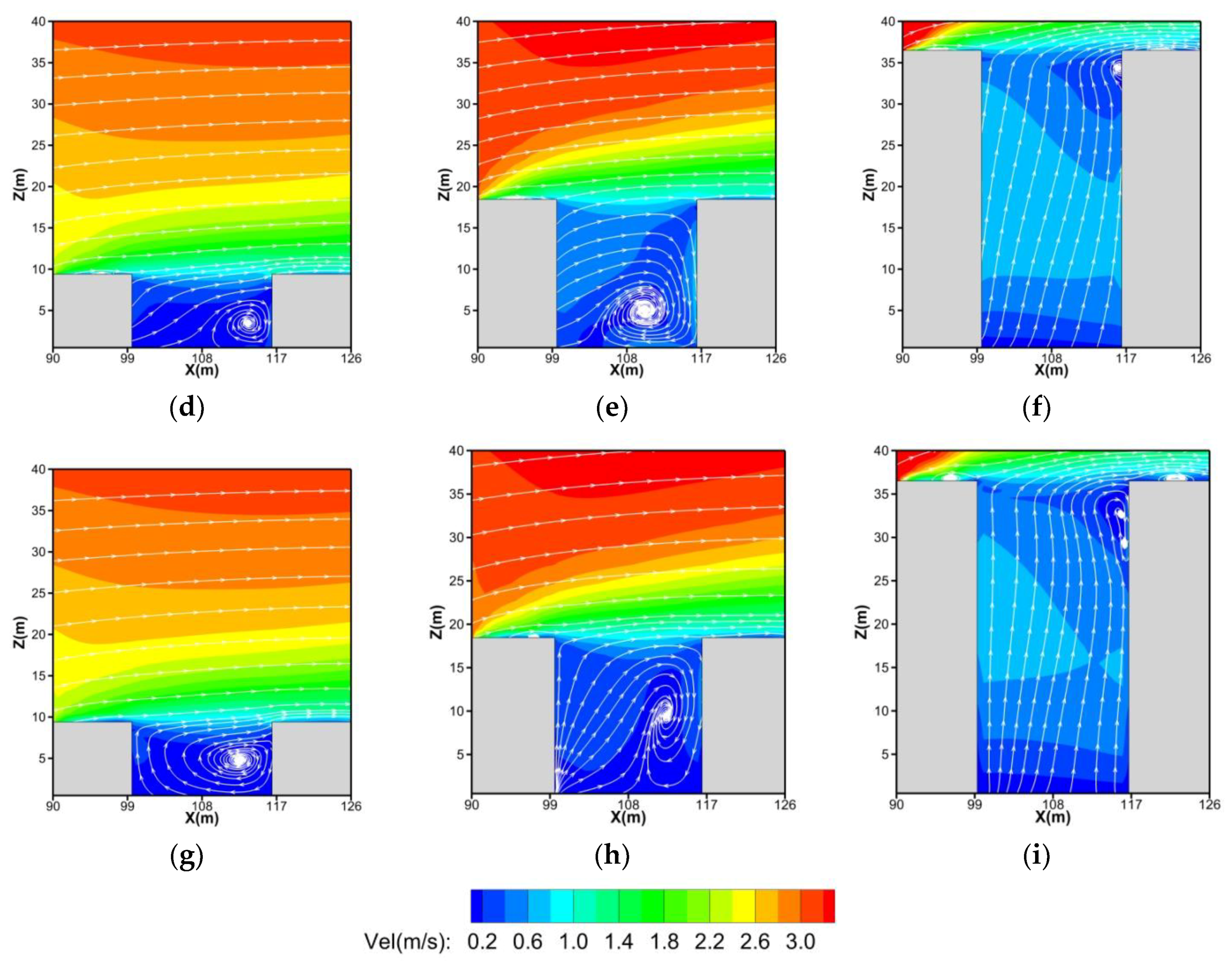
3.1. Airflow Fields with GRs and GWs

Figure 6 shows the streamline fields and wind velocities at y = 140 m in H/W = 0.5, 1.0, and 2.0 with non-greening scenarios, GRs and GWs with LADs of 6.0 m²/m³ and greenery coverage area of S₃. As seen, LADs and greenery coverage have a minor influence on the airflow field in street canyons both in GRs or GWs, and three greenery coverage areas with LADs have similar turbulent phenomena with the same aspect ratio. When airflow encounters the windward façade of the front building, the wind speed abruptly increases at the building’s roof. These images demonstrate that wind speed increases with increasing aspect ratio, because the dragging force exerts a strong influence within deep street canyons and strengthens momentum and kinetic energy. For H/W = 0.5 and 1.0, a clockwise vortex appears within the street canyon in each scenario as reported by Li et al and Bright et al. [55,56]. Due to the influence of GRs and GWs, the shape of the vortex differs compared with the scenario without greened surfaces. When H/W = 0.5, the predominant wind direction is identical to a weakened turbulent effect in street canyons in GRs cases. However, the turbulent effect is obviously strengthened, and the predominant wind direction is from the bottom to the top of the building in GW cases. When H/W = 1.0, turbulence is relatively flat in GR scenarios. Wind speed is slightly higher near the windward façade of the leeward building and the lowest wind speed appears in the turbulent region in the street canyon. GWs could cause the airflow field to change which is represented by the position of vortex moving up, and the predominant wind direction changes from the bottom left to the upper right. For H/W = 2.0, two vertically-aligned clockwise vortices are generated at the rooftops. Airflow fields with two deformable vortices in GRs are significantly affected by impeding vegetation, which causes velocity to increase and vortices to compress. It should be noted that wind speed initially increases and then decreases with building height. GWs, due to vegetation distribution along the vertical wall, have a large effect on the airflow field in the street canyon. As a result of GWs, wind velocity is relatively low and two clockwise vortices are generated in the street canyon.

3.2. Pollutant Dispersion by GRs and GWs

3.2.1. Street-Canyon Concentration Distributions

Figure 7 illustrates the contours of PM₁₀ concentration at y = 190 m in H/W = 0.5, 1.0, and 2.0 with non-greening scenarios, GRs and GWs with LAD of 6.0 m²/m³ and greenery coverage of S₃. As can be seen in Figure 7, PM₁₀ concentrations disperse toward windward walls for the non-greening scenarios, and their dispersion patterns change as vegetation is implemented in the roofs and walls such that their concentrations on the leeward walls decrease with increasing street canyon aspect ratio. This is because the deposition effect of vegetation on GRs (GWs) and the shading effect of the windward building increasing with the aspect ratio, which creates greater drag forces within street canyons. For these reasons, the smallest values are found in H/W = 2.0 scenarios. At the same time, concentrations along the leeward façade of the front building are smaller in comparison to the windward façade of the back building. For H/W = 0.5, concentration distributions in GRs are similar to the non-greening case. The smallest concentrations exist where vegetation was installed in GWs. Concentrations decrease at the street corner for H/W = 1.0 cases with GRs and GWs. In the H/W = 2.0 scenario, concentrations along vertical profile of the street corner remains lower for GRs cases. Concentration distributions have a similar trend of increasing with building height.

Averaged PM₁₀ concentrations in street canyons were calculated to determine how much they were reduced by GRs and GWs. Averaged concentrations in street canyons were calculated using concentrations within three-dimensional space of the street canyons, from 99 to 117 m on the X axis, from 90 to 190 m on the Y axis, and from 0 to 9 m, 18 m, and 36 m, respectively, on the Z axis for scenarios simulating three aspect ratios. Averaged concentrations plotted against LADs and greenery coverage are depicted in Figure 8. This approach reveals that averaged concentrations are lower in GWs than that in GRs. With the same greenery coverage, concentration differences between GWs and GRs gradually decreases as LAD increases. This also indicated that averaged concentration in GRs is higher than in cases with non-greening, especially within deep canyon of H/W = 2.0 (Figure 8c). Thus, GRs in deep street canyons can cause the concentrations to increase within the street canyon.

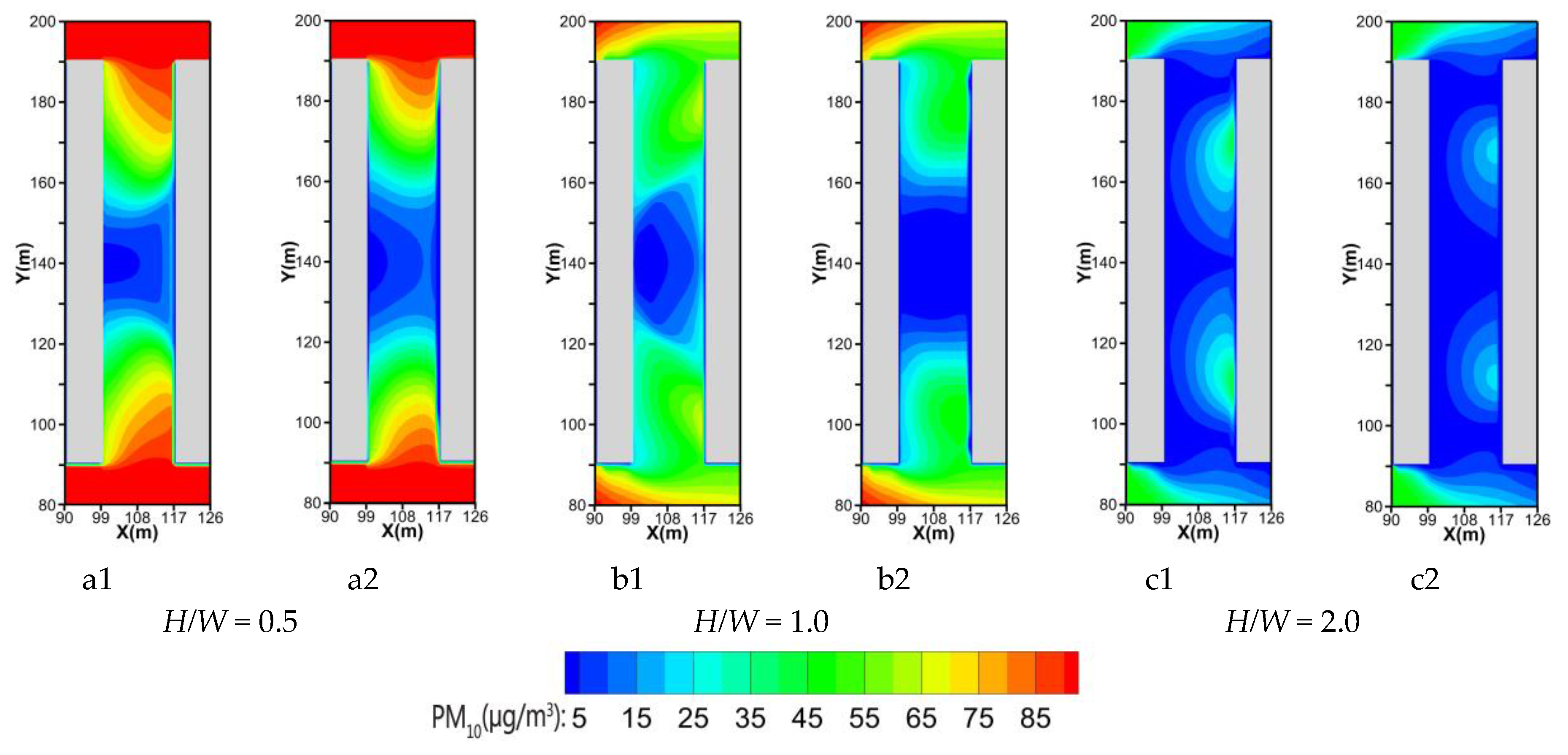
3.2.2. Pedestrian-level Concentration Distributions

Figure 9 depicts the contours of PM₁₀ concentration in H/W = 0.5, 1.0, and 2.0 with GRs and GWs at the pedestrian level (1.5 m height), a level where is essential for pedestrians’ outdoor breathing. The concentrations decrease with increasing aspect ratio due to the building shading effect. For H/W = 0.5 and 1.0, particle concentrations are lower in the middle region of the street canyon, are higher at the street corner, and the range of low concentration is clearly larger in all H/W = 2.0 cases. For H/W = 0.5, particle concentrations are clearly lower in street canyon center with GRs and GWs are present. Additionally, their distributions are approximate. However, lower concentrations exist in the region close to the wall façade for GWs. Concentrations are slightly lower and clearly decrease in the center region for H/W = 1.0. Furthermore, this comparison indicates that concentrations are lowest at the pedestrian level with GWs when H/W = 2.0. Based on the comparison of concentration distributions under three aspect ratios, the influence of GRs on particle concentration gradually weakens as the aspect ratio increases at the pedestrian level, but strengthens with GWs.

The averaged concentrations against LAD and greenery coverage at the pedestrian level (1.5 m height) are illustrated in Figure 10. Averaged concentrations at the pedestrian level were calculated using concentrations at Z = 1.5 m within street canyons, from 99 to 117 m on the X axis, and from 90 to 190 m on the Y axis. The averaged concentrations decrease with increasing aspect ratios. Concentrations in GWs are higher for H/W = 0.5, in comparison to GRs. Moreover, with the same LAD, concentrations gradually decrease as greenery coverage and LAD increase. However, when greening areas are S₂ and S₃, the concentration changes are smaller as LAD increases from 3.5 to 6.0 m²/m³. Concentration changes show similar trends in GRs. Additionally, concentration differences among the three LADs become more obvious as greenery coverage increased in area. For H/W = 1.0, averaged concentrations of GWs decline greatly as LAD and greenery coverage increase. While, the effect of GRs on pollutant absorption is unclear due to the distance from the street canyon, concentration differences between GWs and GRs increases with greenery coverage and LADs. This phenomenon indicates, that for H/W = 1.0, the greater the LADs and greenery coverage, the stronger the deposition effect exerted by GWs. When H/W = 2.0, the averaged concentrations in GWs are clearly lower than that in GRs. However, concentration differences are not very clear as LADs and greenery coverage increase with GWs (or GRs). Nevertheless, the overall tendency remains consistent; concentrations decrease with increasing LADs and greenery coverage.

Based on the above comparisons, PM₁₀ concentrations with GRs are lower in H/W = 0.5. However, for H/W = 1.0 and 2.0, the deposition effect of GWs is stronger, and differences between GWs and GRs are larger compared to that for H/W = 0.5. The differences among LADs are significant with the greenery coverage of S₃ where the absolute value reaches 6.1 μg/m³. In addition, the absolute differences between GWs and GRs ranges from 1.0 to 2.3 μg/m³ for H/W = 0.5, and from 2.0 to 3.1 μg/m³ for H/W = 2.0 cases, respectively.

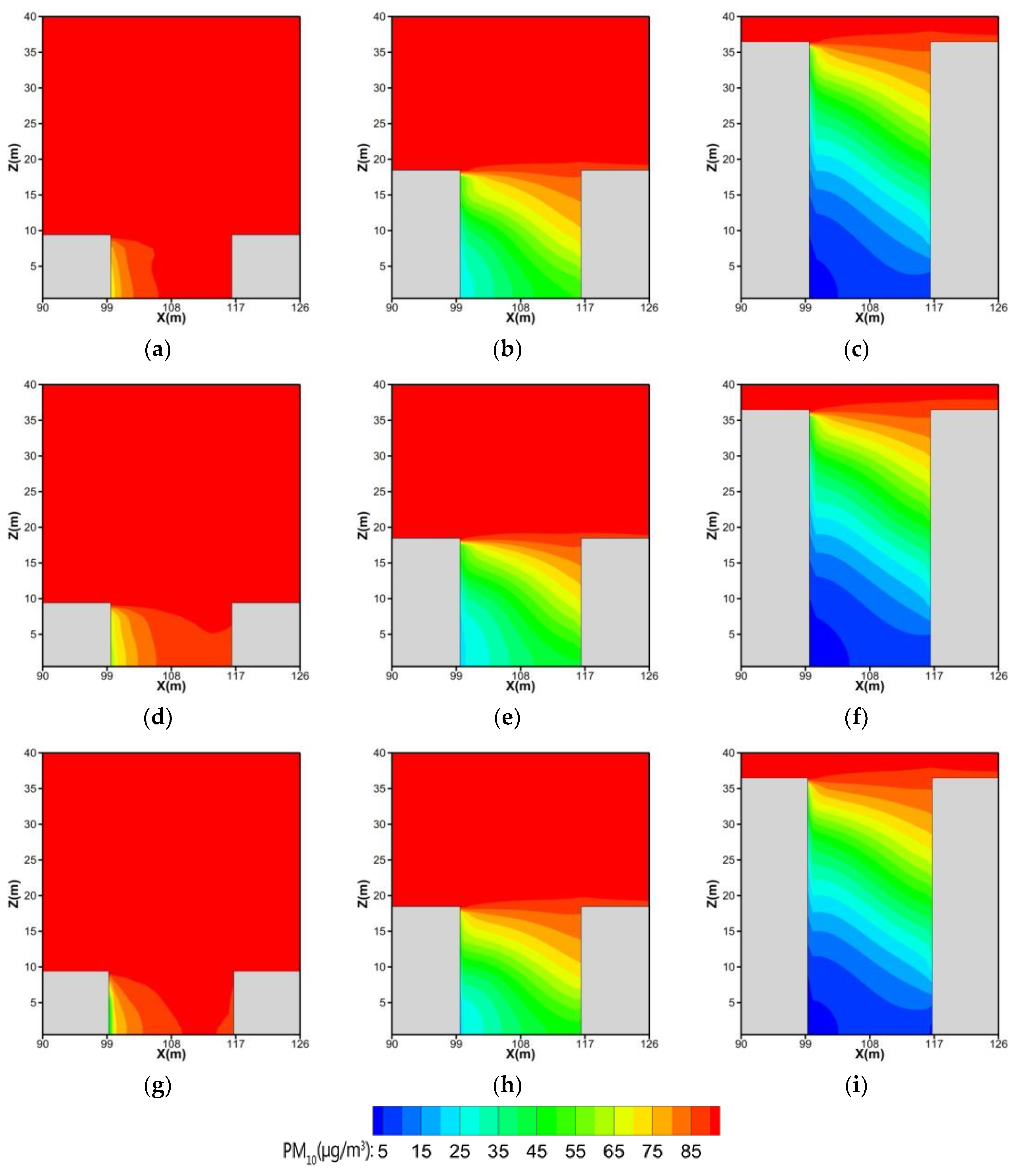
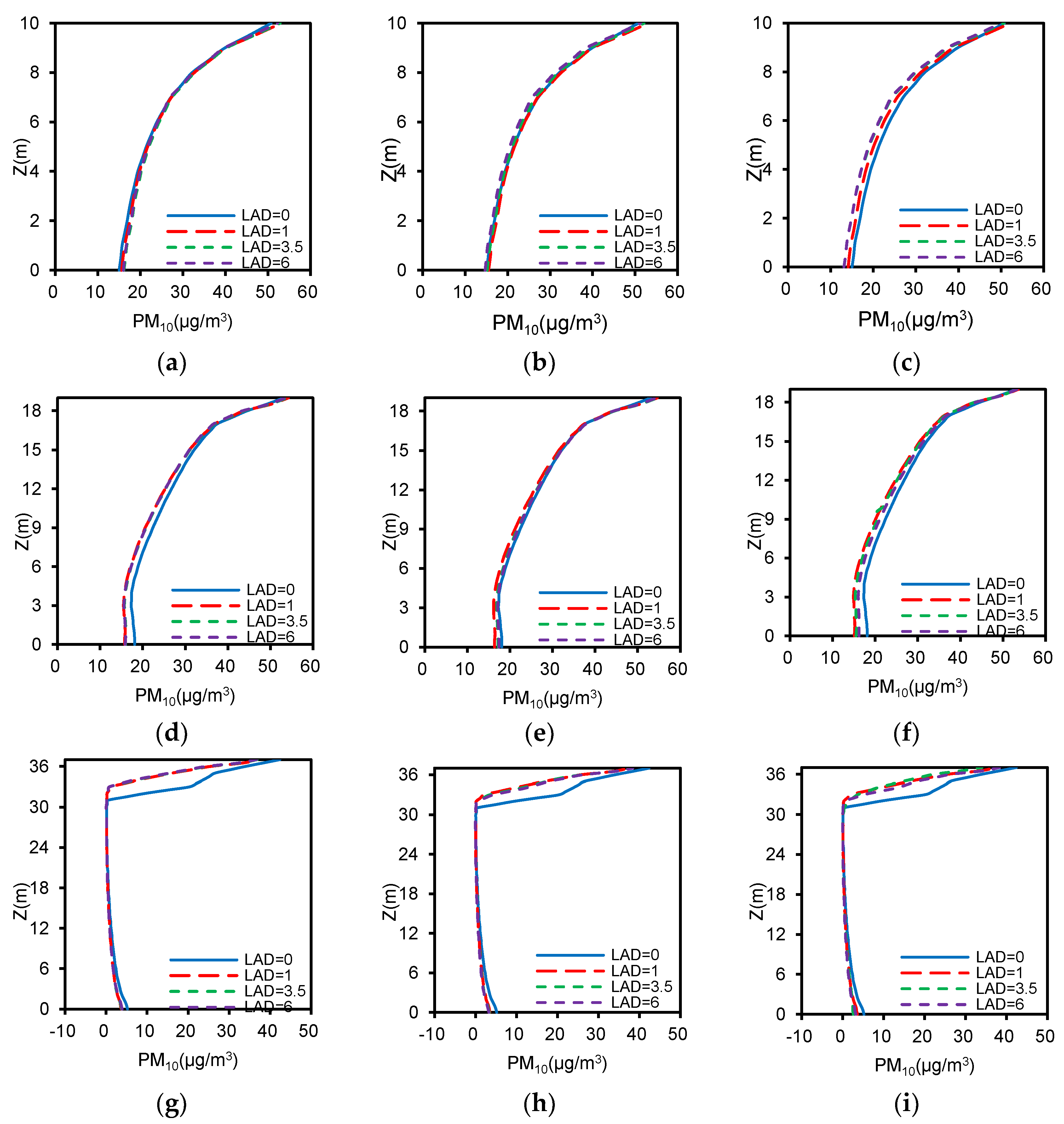
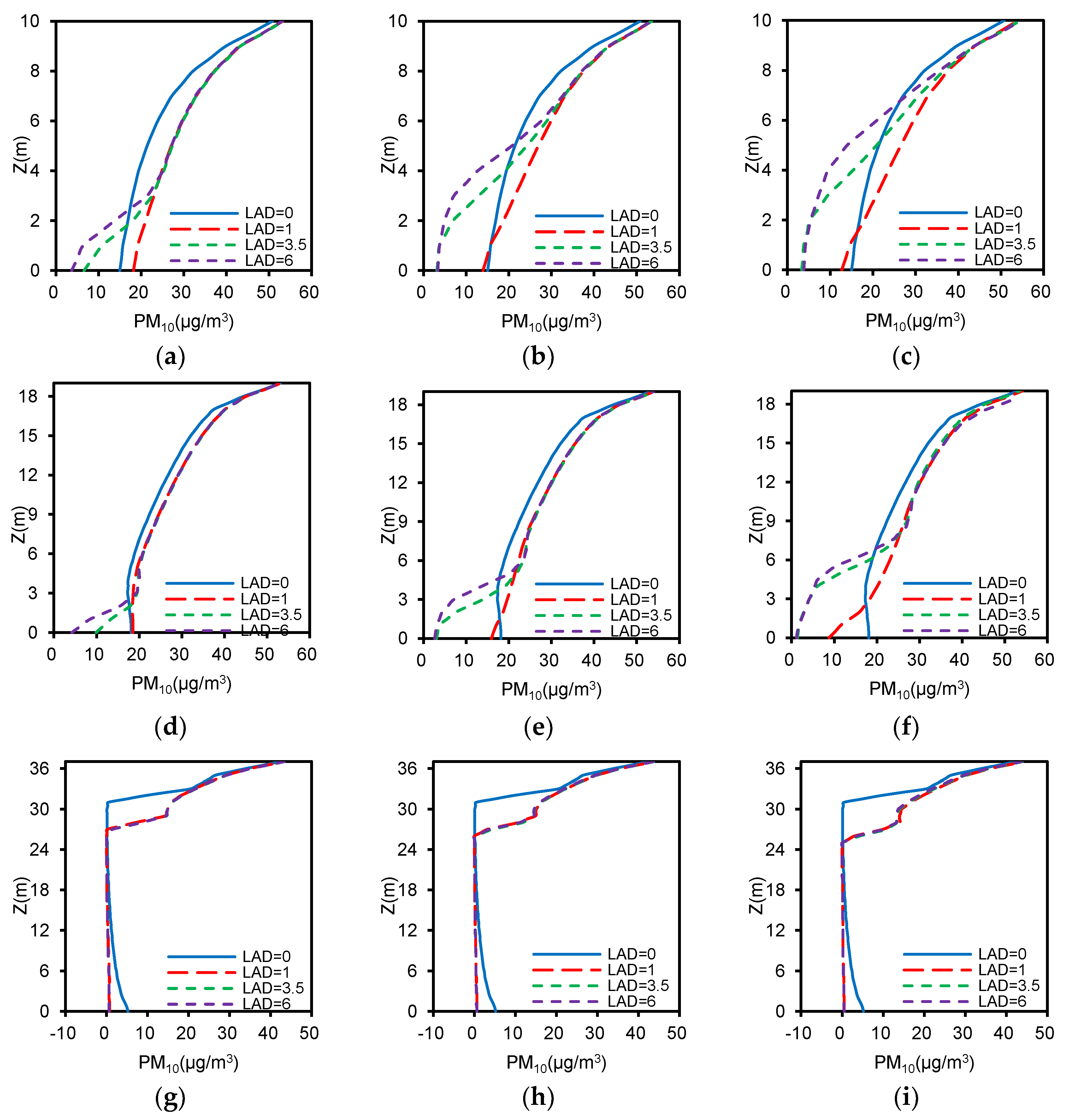
3.2.3. Vertical Concentration Distributions

Figure 11 depicts the PM₁₀ concentrations along a vertical line located at the canyon-center on windward wall of back building with GRs. In scenarios where H/W = 0.5, particle concentrations without greening are slightly smaller at the same level with S₁ greening coverage (Figure 11a). Increasing the greenery area to S₃ causes concentrations of various LADs to be smaller than in non-greening scenarios (Figure 11c). It is also observed that concentration differences, plotted against LADs at the same level, increase with increased greenery coverage. For H/W = 1.0, particle concentrations in non-greening cases are greater than that with greening. Particle concentration differences among various scenarios are all small when Z > 17 m. The concentration changes are identical among LADs of 1.0, 3.5, and 6.0 m²/m³ in S₁. Increasing to S₂, concentrations among various LADs differ slightly. However, when greening coverage is S₃, the concentrations are clearly different at different LADs (ranked as: C_(LAD=1) < C_(LAD=3.5) < C_(LAD=6) < C_(LAD=0)). In the scenario where H/W = 2.0, concentrations of LAD = 0 increase abruptly because of wind deflection created by windward buildings above 31 m. Due to the deposition effect of vegetation, concentrations of LAD = 0 are significantly higher than other LADs and above 31 m. Furthermore, the concentrations increase rapidly at about 33 m with greening scenarios because GRs affects airflow fields and increase the shading effect of windward buildings. Particle concentrations for each LAD (except for non-greening scenarios) are almost identical above 33 m but with smaller differences. Analysis of mentioned line along building façade indicates that maximum particle concentrations are found above the roof because wind deflection causes the particle concentration to increase rapidly near the building tops.

Figure 12 shows the PM₁₀ concentrations along a vertical line located at the canyon-center on windward wall of back building with GWs. For aspect ratios where H/W = 0.5, concentrations with LAD = 1.0 m²/m³ are often higher than that with LAD = 0 at the same height. Additionally, particle concentrations at the bottom of the street canyon space decrease with increasing greenery coverage for LADs. Analysis of Figure 12a shows that particle concentrations under non-greening scenarios are clearly lower than that in GWs when Z > 2.5 m. This phenomenon demonstrates that the aerodynamic effect of GWs is greater than the deposition effect when Z > 2.5 m under S₁, suggesting that GWs perform well at higher PM₁₀ concentrations. However, the concentrations within LAD = 1.0 m²/m³ are all lower than those with LAD = 0 at the same height due to smaller aerodynamic effects. When Z > 5 m, concentrations are all higher in greening scenario compared with non-greening scenario for greater aerodynamic effect of GWs (Figure 12b). In scenarios of H/W = 1.0, concentration is higher with S₁ for LAD = 1.0 m²/m³ compared with non-greening situation (Figure 12d). Concentrations are both greater than non-greening cases at the same level when Z > 1 m under S₂ and Z > 2.5 m under S₃ (Figure 12e,f). Similar to H/W = 0.5 cases, concentrations decrease with increasing greenery coverage for each LAD at the bottom of the street canyon (except for the non-greening scenario). In the case of H/W = 2.0, the concentrations gradually decrease with building height and reach their minimum at Z = 31 m, then abruptly increase when LAD = 0. Nevertheless, when Z < 26 m, particle concentrations are uniform in GWs, which are smaller than non-greening scenarios, have obvious effects on reducing particles. However, concentrations clearly increase in GWs above 26 m and grow larger than in cases where LAD = 0.

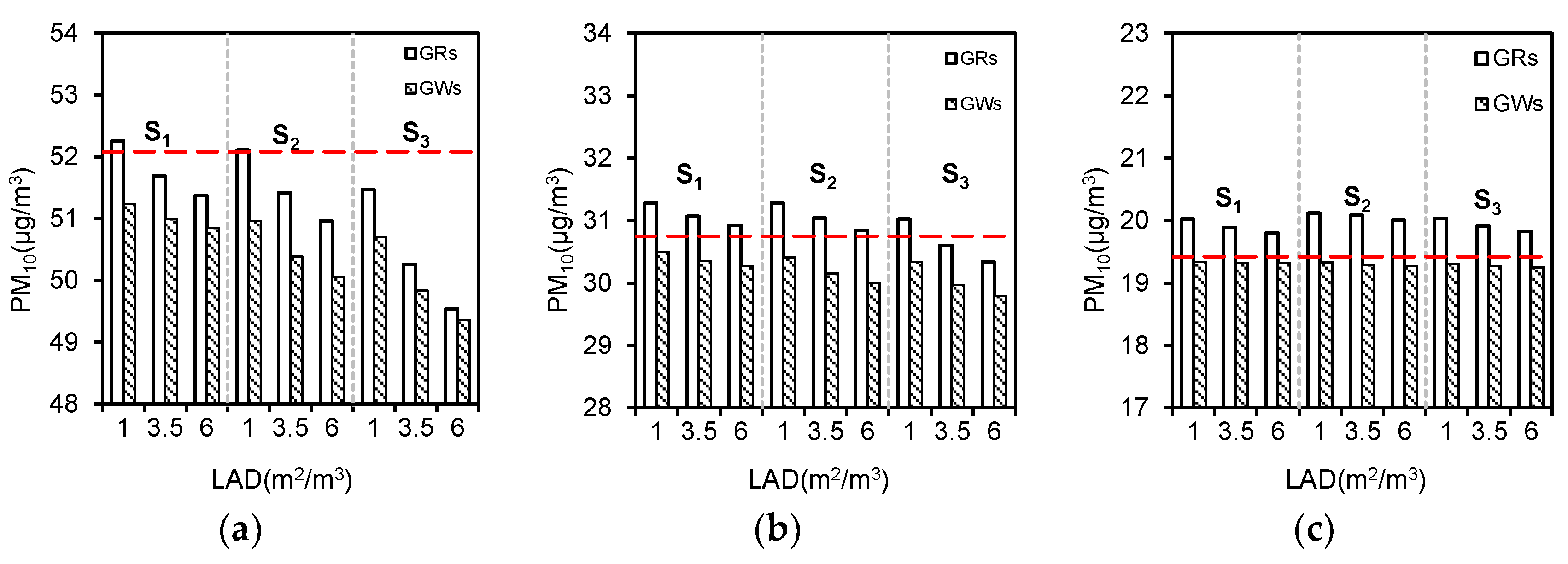
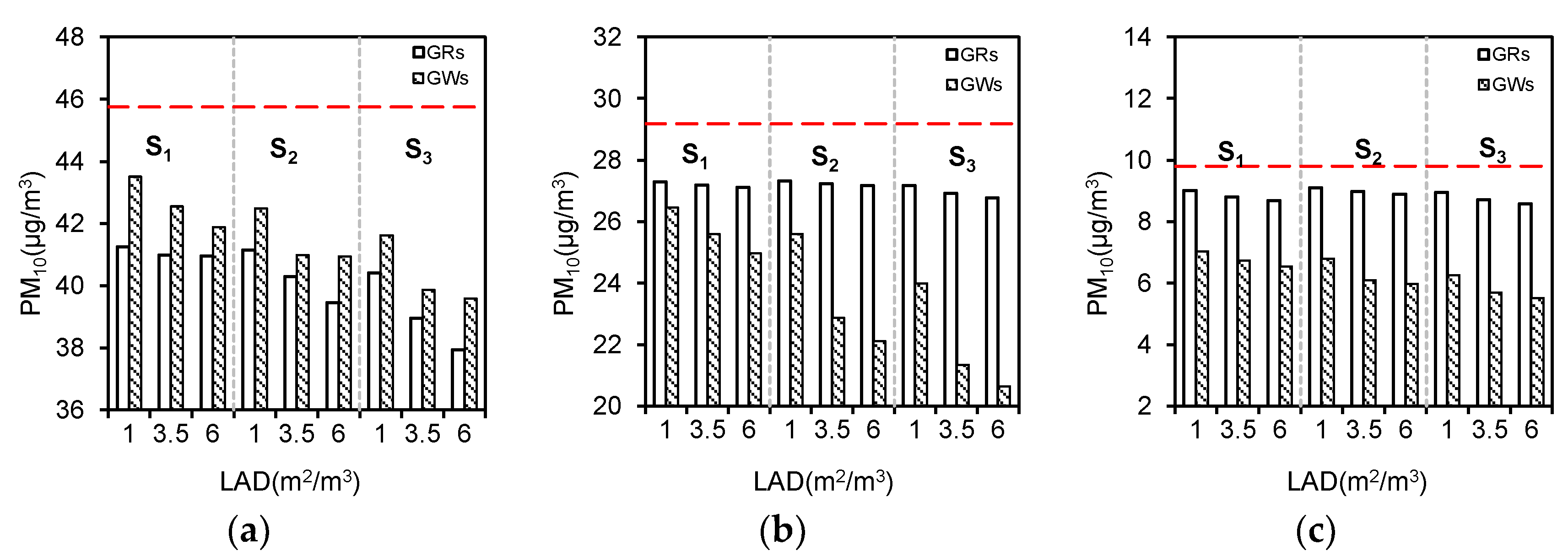
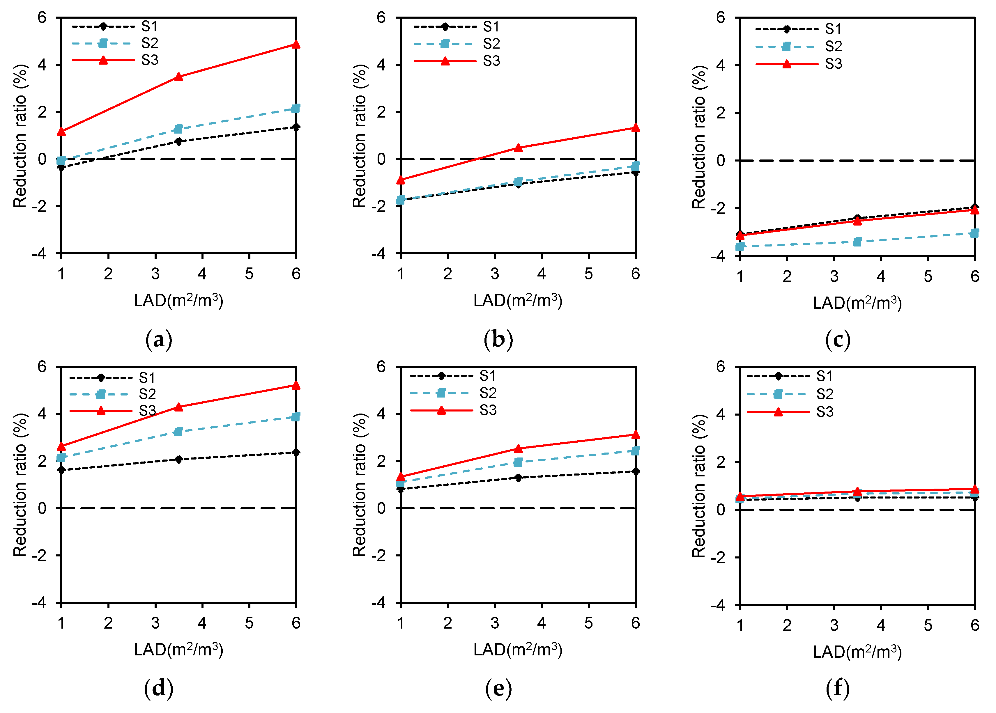
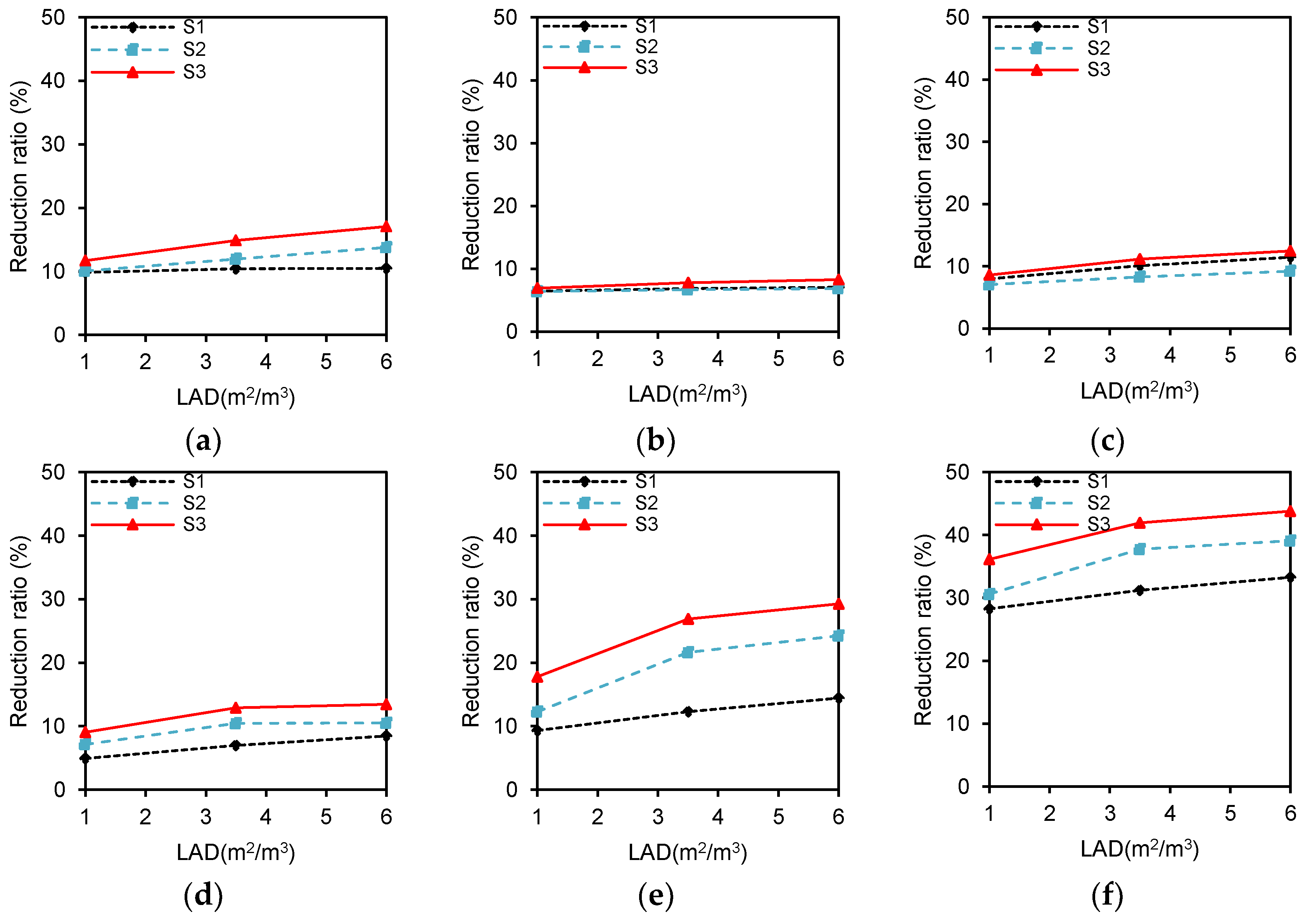
3.3. PM₁₀ Reduction Ratio with GRs and GWs

The averaged PM₁₀ concentrations with and without greening were calculated to confirm their efficiency to reduce particulate pollution. Reduction ratios of averaged concentration against LADs and greenery coverage for three aspects ratios with GRs (Figure 13a–c) and GWs (Figure 13d–f) are illustrated. The reduction ratio is calculated as:

$$\omega =\left(\frac{C_{ave,non-greening}-C_{ave}}{C_{ave,non-greening}}\right)\times 100\%$$

(17)

where ω is the reduction ratio that describes the reduction capability of greening on PM₁₀ concentrations. C_{ave,non-greening} and C_ave are the averaged concentrations at non-greening and GRs (GWs) scenarios, respectively.

The results presented in Figure 13 indicate that the reduction ratios increase with LADs and greenery coverage at the same aspect ratio. The reduction effect on particles due to GWs, performing all positive reduction ratio values, is clearly stronger than that of GRs under the same condition for the domain. Reduction ratios of averaged concentrations in GRs are all negative within street canyons for H/W = 2.0. GRs increase the street-canyon concentrations at this aspect ratio. Two positive values exist when H/W = 1.0, being 0.5% and 1.3%, respectively, where LAD = 3.5 m²/m³ and 6.0 m²/m³ with S₃. For H/W = 0.5, most reduction ratios are positive values. With the greenery coverage of S₃, the reduction ratio increases rapidly as LAD increases from 1.0 to 3.5 m²/m³. However, when it changes from 3.5 to 6.0 m²/m³, the reduction ratio increases slightly, and the ratio reaches the maximum value of 4.9% when LAD = 6.0 m²/m³.

Figure 13 also shows that the reduction ratio clearly increases with greenery coverage with the same LAD for H/W = 0.5. Reduction ratio difference increases as LAD and coverage greenery increase. When H/W = 1.0, reduction ratios have a similar trend as that with aspect ratio of 0.5, and differences among LADs increase significantly with a greenery increases. For H/W = 2.0, reduction ratios of particle concentrations under different scenarios are all low, and LAD and greenery coverage can cause minor concentration reduction within a range of just 0.4–0.9%.

Figure 14 depicts the reduction ratio of averaged concentration at the pedestrian level. The reduction ratio, expressed as Equation 17, estimates the attenuation efficiency of PM₁₀ for GRs and GRs. It could be seen that both GRs and GWs have significant effects to reduce the pedestrian-level concentrations, and GRs strongly reduce concentrations when H/W = 0.5 (Figure 14a). The effect is slightly weaker in H/W = 2.0 scenarios and is the weakest when H/W = 1.0 (Figure 14b,c). The reduction effect of GWs is clearly strengthened as the aspect ratio increases. Reduction ratios of GRs are higher than GWs under the same conditions which suggests that GRs have better deposition effects when H/W = 0.5. However, when H/W ratios are 1.0 and 2.0, reduction ratios are higher in GWs.

The reduction ratios increase with LADs and greenery coverage under different H/W ratios with GWs. With greenery coverage of S₁, the reduction ratio changes uniformly among LADs for different H/W ratios. For S₂ and S₃, the reduction ratio increases significantly as LAD changes from 1.0 to 3.5 m²/m³, but increases only slightly from 3.5 to 6.0 m²/m³. In the scenario where H/W = 0.5, the reduction ratio ranges from 4.9% to 13.5%. The reduction ratio difference among greenery coverage areas is the largest when H/W = 1.0. Nevertheless, when H/W = 1.0 and 2.0, the reduction ratio ranges are from 9.3 to 29.3%, and from 28.3 to 43.8%, respectively.

Results of this research demonstrated that the GRs and GWs can effectively cut PM₁₀ pollution at the pedestrian level, especially within deep street canyons. These findings add to the conclusions drawn by Moradpour et al. [13]. The comparison of GRs and GWs demonstrated that the aerodynamic effect of GRs is greater than the deposition effect, resulting in decreasing airflow in the street canyons, and leading to an increase in concentrations in the whole domain, especially when H/W = 2.0. Additionally, by using wind tunnel experiments and numerical simulations, Buccolieri et al. demonstrated that the aspect ratio of street canyons was a more crucial parameter than plant morphology, positioning and arrangement [57]. Our simulation study also showed that the reduction ratio of PM₁₀ was strongly despondent upon increasing aspect ratios of street canyons, thus consolidating Buccolieri’s conclusion.

This study quantified the aerodynamic and deposition effects of GRs and GWs on PM₁₀ dispersion in street canyons. The results indicate that judicious design of vegetation and urban morphology can yield improvements in air quality in dense urban streets. However, our research has some limitations. First, particle dispersion is modeled as a continuum and assumed to have no effect on airflow turbulence in our simulations, so it was the steady state result. However, wind flow in actual environments is transient. Even a constant condition results in transient vortex shedding under certain configurations that are important for pollutant mixing [58]. Thus, experimental validation of our quantitative results is needed. Second, the pollutants are wind dispersed in this study. However, there are other mechanisms under thermally driven conditions that also disperse particles that we do not consider. Further study should consider the non-isothermal cases with solar radiation and convective heat transfer between buildings and vegetation. Third, GWs in our models were simulated as entire walls with no consideration of window-wall ratios on building façades. Further research should take this condition into account for simulating a more realistic environment. Fourth, this study compared herbaceous vegetation on GRs and GWs affecting the street-canyon airflow and pollutant dispersion. Except for grass, small trees and shrubs are commonly included in GRs, thus, more comparative studies should consider the influence of small trees and shrubs. Fifth, this study was done under the condition of wide width building, such as more than 100 m. It must be accepted that the building width has much effect on all calculated results. Thus, the conclusions drawn below may be not applicable for the actual building of less than 100 m width. Finally, a previous study indicated that an accurate assessment of the porosity of plant canopies with height could precisely describe the LAD and drag coefficient [59], and the drag coefficients remained nearly constant for Reynolds number greater than 6 × 10⁴ [60]. In this CFD simulation, only herbaceous vegetation with the height of 0.3 m was considered. Further research should pay more attention to the relationship between the LAD and drag coefficient concerning the small trees and shrubs.

4. Conclusions

In this study, the dispersion of coarse particles in urban street canyons with GWs and GRs were studied at three levels of street canyon aspect ratios (0.5, 1.0, and 2.0). Vegetation on GWs and GRs with different coverage areas (300, 600, and 900 m²), and leaf area densities (1.0, 3.5, and 6.0 m²/m³) was considered, and their effects on airflow fields and PM₁₀ dispersion were investigated by CFD simulations coupled with the RANS model and revised generalized drift flux model. From the results, under the wide width building of more than 100 m, the following conclusions can be drawn:

(1)

Turbulence on a street canyon vertical plane is greater with GWs, and its influence on airflow field and turbulence is stronger than that with GRs. While the roof turbulence of GRs is large, it is manifested by weakened turbulent effects and increasing wind speed in the street canyon. The flow structure contains one clockwise vortex within H/W = 0.5 and 1.0, and two vertically-aligned vortices in GWs within H/W = 2.0.

(2)

Particle concentrations within the street canyon on a vertical line at windward façade of the back building changes greatly with building height. For GRs, particle concentration differences among LADs increase with the increasing greenery coverage when H/W = 0.5 and 1.0. Particle concentrations of LAD = 0 are significantly higher than in other LADs above 31 m, and increase abruptly with height above 31 m when H/W = 2.0. For GWs, particle concentrations at the bottom of street canyon decrease with increasing greenery coverage for the same LAD in H/W = 0.5 and 1.0 cases. In the case of H/W = 2.0, the concentrations gradually decrease with building height and reach their minimum at Z = 31 m.

(3)

At the pedestrian level, the effect of GRs on reducing particle concentrations is weakened with increasing H/W compared to that of GWs. For H/W = 0.5, the concentration is lower within GRs ranging from 37.9 to 41.3 μg/m³, and the reduction ratio is larger than GWs with a maximum reduction ratio of 17.1%. For H/W = 1.0 and 2.0, the concentration within GRs is larger than that of GWs, with maximum reduction ratios of 29.3% and 43.8%, respectively.

(4)

Particle concentrations in GWs are lower than those in GRs across the entire spatial domain in the same scenarios. GRs result in higher averaged concentrations compared with the non-greening case where H/W = 2.0. Averaged concentrations decline within creasing LADs and greenery coverage areas, especially the H/W. With the aspect ratio held constant, the reduction ratio between GRs and GWs increases with the increasing LAD and greenery coverage areas.

In this study, the urban street canyon was composed of two parallel and contiguous building complexes with the street canyon length of 100 m. The numerical analysis for modeling airflow and PM₁₀ dispersion for building complexes suggests that GWs are more effective than GRs in reducing street-canyon PM₁₀ with equal greenery coverage area and aspect ratio, and the averaged PM₁₀ concentrations declined with increasing LADs and greenery coverage areas, especially the H/W. Additionally, the reduction ratio of GRs is greater than GWs for H/W = 0.5. However, for H/W = 1.0 and 2.0, the concentrations within GWs are lower than GRs at the pedestrian level. These results indicate that urban planners should judiciously consider the implementation of GWs and GRs by analyzing each particular scenario combined with multiple, interacting factors, i.e., block morphology, vegetation types, planting density, coverage area, and location of pollutant sources (e.g., traffic-originated, atmospheric transportation) with the purpose of improving air quality in urban street canyons.

References

1. UN-Habitat. Urbanization and Development: Emerging Futures. In World Cities Report; United Nations Human Settlements Programme (UN-Habitat): Nairobi, Kenya, 2016; Available online: http://wcr.unhabitat.org/main-report (accessed on 1 January 2017).
2. Hong, B.; Lin, B. Numerical studies of the outdoor wind environment and thermal comfort at pedestrian level in housing blocks with different building layout patterns and trees arrangement. Renew. Energy 2015, 73, 18–27. [Google Scholar] [CrossRef]
3. Pierangioli, L.; Cellai, G.; Ferrise, R.; Trombi, G.; Bindi, M. Effectiveness of passive measures against climate change: Case studies in Central Italy. Build. Simul. 2017, 10, 459–479. [Google Scholar] [CrossRef]
4. Rowe, D.B. Green roofs as a means of pollution abatement. Environ. Pollut. 2011, 159, 2100–2110. [Google Scholar] [CrossRef] [PubMed]
5. Berardi, U.; GhaffarianHoseini, A.H.; GhaffarianHoseini, A. State-of-the-art analysis of the environmental benefits of green roofs. Appl. Energy 2014, 115, 411–428. [Google Scholar] [CrossRef]
6. Jayasooriya, V.M.; Ng, A.W.M.; Muthukumaran, S.; Perera, B.J.C. Green infrastructure practices for improvement of urban air quality. Urban For. Urban Green. 2017, 21, 34–47. [Google Scholar] [CrossRef]
7. Gromke, C.; Ruck, B. On the impact of trees on dispersion processes of traffic emissions in street canyons. Bound.-Lay. Meteorol. 2009, 131, 19–34. [Google Scholar] [CrossRef]
8. Buccolieri, R.; Salim, S.M.; Leo, L.S.; Di Sabatino, S.; Chan, A.; Ielpo, P.; de Gennaro, G.; Gromke, C. Analysis of local scale tree–atmosphere interaction on pollutant concentration in idealized street canyons and application to a real urban junction. Atmos. Environ. 2011, 45, 1702–1713. [Google Scholar] [CrossRef]
9. Speak, A.F.; Rothwell, J.J.; Lindley, S.J.; Smith, C.L. Urban particulate pollution reduction by four species of green roof vegetation in a UK city. Atmos. Environ. 2012, 61, 283–293. [Google Scholar] [CrossRef]
10. Janhäll, S. Review on urban vegetation and particle air pollution—Deposition and dispersion. Atmos. Environ. 2015, 105, 130–137. [Google Scholar] [CrossRef]
11. Tong, Z.; Whitlow, T.H.; MacRae, P.F.; Landers, A.J.; Harada, Y. Quantifying the effect of vegetation on near-road air quality using brief campaigns. Environ. Pollut. 2015, 201, 141–149. [Google Scholar] [CrossRef] [PubMed]
12. Yang, J.; Yu, Q.; Gong, P. Quantifying air pollution removal by green roofs in Chicago. Atmos. Environ. 2008, 42, 7266–7273. [Google Scholar] [CrossRef]
13. Currie, B.A.; Bass, B. Estimates of air pollution mitigation with green plants and green roofs using the UFORE model. Urban Ecosys. 2008, 11, 409–422. [Google Scholar] [CrossRef]
14. Moradpour, M.; Afshin, H.; Farhanieh, B. A numerical study of reactive pollutant dispersion in street canyons with green roofs. Build. Simul. 2017, 11, 1–14. [Google Scholar] [CrossRef]
15. Li, J.-F.; Wai, O.W.H.; Li, Y.-S.; Zhan, J.; Ho, Y.-A.; Li, J.; Lam, E. Effect of green roof on ambient CO2 concentration. Build. Environ. 2010, 45, 2644–2651. [Google Scholar] [CrossRef]
16. Baik, J.J.; Kwak, K.H.; Park, S.B.; Ryu, Y.H. Effects of building roof greening on air quality in street canyons. Atmos. Environ. 2012, 61, 48–55. [Google Scholar] [CrossRef]
17. Pugh, T.A.; Mackenzie, A.R.; Whyatt, J.D.; Hewitt, C.N. Effectiveness of green infrastructure for improvement of air quality in urban street canyons. Environ. Sci. Technol. 2012, 46, 7692–7699. [Google Scholar] [CrossRef] [PubMed]
18. Ottelé, M.; van Bohemen, H.D.; Fraaij, A.L.A. Quantifying the deposition of particulate matter on climber vegetation on living walls. Ecol. Eng. 2010, 36, 154–162. [Google Scholar] [CrossRef]
19. Tong, Z.; Baldauf, R.W.; Isakov, V.; Deshmukh, P.; Zhang, K.-M. Roadside vegetation barrier designs to mitigate near-road air pollution impacts. Sci. Total Environ. 2016, 541, 920–927. [Google Scholar] [CrossRef] [PubMed]
20. Perini, K.; Ottelé, M.; Giulini, S.; Magliocco, A.; Roccotiello, E. Quantification of fine dust deposition on different plant species in a vertical greening system. Ecol. Eng. 2017, 100, 268–276. [Google Scholar] [CrossRef]
21. Weerakkody, U.; Dover, J.W.; Mitchell, P.; Reiling, K. Particulate matter pollution capture by leaves of seventeen living wall species with special reference to rail-traffic at a metropolitan station. Urban For. Urban Gree. 2017, 27, 173–186. [Google Scholar] [CrossRef]
22. Tong, Z.; Whitlow, T.H.; Landers, A.; Flanner, B. A case study of air quality above an urban roof top vegetable farm. Environ. Pollut. 2016, 208, 256–260. [Google Scholar] [CrossRef] [PubMed]
23. Kessler, R. Green walls could cut street-canyon air pollution. Environ. Health Persp. 2013, 121, 14. [Google Scholar] [CrossRef] [PubMed]
24. Morakinyo, T.E.; Lam, Y.F.; Hao, S. Evaluating the role of green infrastructures on near-road pollutant dispersion and removal: Modelling and measurement. J. Environ. Manag. 2016, 182, 595–605. [Google Scholar] [CrossRef] [PubMed]
25. Pochee, H.; Johnston, I. Understanding design scales for a range of potential green infrastructure benefits in a London Garden City. Build. Serv. Eng. Res. Technol. 2017, 38, 728–756. [Google Scholar] [CrossRef]
26. Buccolieri, R.; Santiago, J.; Rivas, E.; Sanchez, B. Review on urban tree modelling in CFD simulations: Aerodynamic, deposition and thermal effects. Urban For. Urban Green. 2018, 31, 212–220. [Google Scholar] [CrossRef]
27. Franke, J.; Hellsten, A.; Schlunzen, K.H.; Carissimo, B. The COST 732 best practice guideline for CFD simulation of flows in the urban environment: A summary. Int. J. Environ. Pollut. 2011, 44, 419–427. [Google Scholar] [CrossRef]
28. Amorim, J.H.; Rodrigues, V.; Tavares, R.; Valente, J.; Borrego, C. CFD modeling of the aerodynamic effect of trees on urban air pollution dispersion. Sci. Total Environ. 2013, 461, 541–551. [Google Scholar] [CrossRef] [PubMed]
29. Sanz, C. A note on k-epsilon modelling of vegetation canopy air-flows. Bound.-Lay. Meteorol. 2003, 108, 191–197. [Google Scholar] [CrossRef]
30. Katul, G.G.; Mahrt, L.; Poggi, D.; Sanz, C. One- and two-equation models for canopy turbulence. Bound.-Lay. Meteorol. 2004, 113, 81–109. [Google Scholar] [CrossRef]
31. Endalew, A.M.; Hertog, M.; Delele, M.A.; Baetens, K.; Persoons, T.; Baelmans, M.; Ramon, H.; Nicolai, B.M.; Verboven, P. CFD modelling and wind tunnel validation of airflow through plant canopies using 3D canopy architecture. Int. J. Heat Fluid Flow 2009, 30, 356–368. [Google Scholar] [CrossRef]
32. Ji, W.; Zhao, B. Numerical study of the effects of trees on outdoor particle concentration distributions. Build. Simul. 2014, 7, 417–427. [Google Scholar] [CrossRef]
33. Zhao, B.; Chen, C.; Tan, Z. Modeling of ultrafine particle dispersion in indoor environments with an improved drift flux model. J. Aerosol Sci. 2009, 40, 29–43. [Google Scholar] [CrossRef]
34. Bell, J.N.B.; Treshow, M. Air Pollution and Plant Life, 2nd ed.; John Willey & Sons, Ltd.: West Sussex, UK, 2003. [Google Scholar]
35. Tominaga, Y.; Mochida, A.; Yoshie, R.; Kataoka, H.; Nozu, T.; Yoshikawa, M.; Shirasawa, T. AIJ guidelines for practical applications of CFD to pedestrian wind environment around buildings. J. Wind Eng. Ind. Aerodyn. 2008, 96, 1749–1761. [Google Scholar] [CrossRef]
36. Roache, P.J. Perspective: A method for uniform reporting of grid refinement studies. J. Fluids Eng. 1994, 116, 405–413. [Google Scholar] [CrossRef]
37. Nowak, D.J.; Crane, D.E.; Stevens, J.C. Air pollution removal by trees and shrubs in the United States. Urban For. Urban Green. 2006, 4, 115–123. [Google Scholar] [CrossRef]
38. Jeanjean, A.P.R.; Monks, P.S.; Leigh, R.J. Modelling the effectiveness of urban trees and grass on PM2.5 reduction via dispersion and deposition at a city scale. Atmos. Environ. 2016, 147, 1–10. [Google Scholar] [CrossRef]
39. Chang, J.; Hanna, S. Air quality model performance evaluation. Meteorol. Atmos. Phys. 2004, 87, 167–196. [Google Scholar] [CrossRef]
40. Hanna, S.; Chang, J. Acceptance criteria for urban dispersion model evaluation. Meteorol. Atmos. Phys. 2012, 116, 133–146. [Google Scholar] [CrossRef]
41. Hong, B.; Qin, H.; Lin, B. Prediction of wind environment and indoor/outdoor relationships for PM2.5 in different building–tree grouping patterns. Atmosphere 2018, 9, 39. [Google Scholar] [CrossRef]
42. Zaid, S.M.; Perisamy, E.; Hussein, H.; Myeda, N.E.; Zainon, N. Vertical Greenery System in urban tropical climate and its carbon sequestration potential: A review. Ecol. Indic. 2018, 91, 57–70. [Google Scholar] [CrossRef]
43. Zhang, L.; Moran, M.D.; Maker, P.A.; Brook, J.R.; Gong, S. Modelling gaseous dry deposition in AURAMS: A unified regional air quality modelling system. Atmos. Environ. 2002, 36, 537–560. [Google Scholar] [CrossRef]
44. Whittinghill, L.J.; Rowe, D.B.; Schutzki, R.; Cregg, B.M. Quantifying carbon sequestration of various green roof and ornamental landscape systems. Landsc. Urban Plan. 2014, 123, 41–48. [Google Scholar] [CrossRef]
45. Li, G.; Ding, S.; Zhou, X. Ecological effects of the twelve species for vertical greening in South China. J. South China Agric. Univ. 2009, 29, 11–15. (In Chinese) [Google Scholar]
46. Litschke, T.; Kuttler, W. On the reduction of urban particle concentration by vegetation—A review. Meteorol. Zeit. 2008, 17, 229–240. [Google Scholar] [CrossRef]
47. Freer-Smith, P.H.; Beckett, K.P.; Taylor, G. Deposition velocities to Sorbus aria, Acer campestre, Populus deltoides x trichocarpa ‘Beaupré’ Pinus nigra and x Cupressocyparis leylandii for coarse, fine and ultra-fine particles in the urban environment. Environ. Pollut. 2005, 133, 157–167. [Google Scholar] [CrossRef] [PubMed]
48. Petroff, A.; Zhang, L. Development and validation of a size resolved particle dry deposition scheme for application in aerosol transport models. Geosci. Model Dev. 2010, 3, 753–769. [Google Scholar] [CrossRef]
49. Oke, T.R. Street design and urban canopy layer climate. Energy Build. 1988, 11, 103–113. [Google Scholar] [CrossRef]
50. Hefny, M.M.; Ooka, R. CFD analysis of pollutant dispersion around buildings: Effect of cell geometry. Build. Environ. 2009, 44, 1699–1706. [Google Scholar] [CrossRef]
51. Xue, F.; Li, X. The impact of roadside trees on traffic released PM10 in urban street canyon: Aerodynamic and deposition effects. Sustain. Cities Soc. 2017, 30, 195–204. [Google Scholar] [CrossRef]
52. Ye, B.; Ji, X.; Yang, H.; Yao, X.; Chan, C.K.; Cadle, S.H.; Chan, T.; Mulawa, P.A. Concentration and chemical composition of PM2.5 in Shanghai for a 1-year period. Atmos. Environ. 2003, 37, 499–510. [Google Scholar] [CrossRef]
53. Beijing Municipal Environmental Monitoring Center (BMEMC). Real-Time Air Quality in Beijing. Available online: http://www.bjmemc.com.cn (accessed on 1 December 2016).
54. Barratt, R. Atmospheric Dispersion Modeling: An Introduction to Practical Applications; Earthscan Publications: London, UK, 2001. [Google Scholar]
55. Li, X.-X.; Britter, R.E.; Norford, L.K.; Koh, T.Y.; Entekhabi, D. Flow and pollutant transport in urban street canyons of different aspect ratios with ground heating: Large-eddy simulation. Bound.-Lay. Meteorol. 2012, 142, 289–304. [Google Scholar] [CrossRef]
56. Bright, V.B.; Bloss, W.J.; Cai, X. Urban street canyons: Coupling dynamics, chemistry and within-canyon chemical processing of emissions. Atmos. Environ. 2013, 68, 127–142. [Google Scholar] [CrossRef]
57. Buccolieri, R.; Gromke, C.; Di Sabatino, S.; Ruck, B. Aerodynamic effects of trees on pollutant concentration in street canyons. Sci. Total Environ. 2009, 407, 5247–5256. [Google Scholar] [CrossRef] [PubMed]
58. King, M.; Gough, H.L.; Halios, C.; Barlow, J.F.; Robertson, A.; Hoxey, R.; Noakes, C.J. Investigating the influence of neighbouring structures on natural ventilation potential of a full-scale cubical building using time-dependent CFD. J. Wind Eng. Ind. Aerod. 2017, 169, 265–279. [Google Scholar] [CrossRef]
59. Desmond, C.J.; Watson, S.J.; Aubrun, S.; Ávila, S.; Hancock, P.; Sayer, A. A study on the inclusion of forest canopy morphology data in numerical simulations for the purpose of wind resource assessment. J. Wind Eng. Ind. Aerodyn. 2014, 126, 24–37. [Google Scholar] [CrossRef] [Green Version]
60. Molina-Aiz, F.D.; Valera, D.L.; Àlvarez, A.J.; Madueño, A. A wind tunnel study of airflow through horticultural crops: Determination of the drag coefficient. Biosyst. Eng. 2006, 93, 447–457. [Google Scholar] [CrossRef]
Figure 1. Location of measurement points (a) and a lateral view of points implemented (b) at the field site.
Sustainability 10 02833 g001
Figure 2. Field measurements of (a) averaged wind velocity and wind direction per hour and (b) averaged PM10 concentrations per hour at point P.
Sustainability 10 02833 g002
Figure 3. Comparisons between normalized PM10 concentrations in field measurements and simulations (dashed lines represent linear fits with linear equations and R2 alongside).
Sustainability 10 02833 g003
Figure 4. Case settings in this study (54 cases were built within three levels of greenery coverage areas, LADs and aspect ratios).
Sustainability 10 02833 g004
Figure 5. The computational domain (schematic diagram of the street canyon with GRs at the level of H/W = 1.0, S = 900m2, and LAD = 6.0 m2/m3).
Sustainability 10 02833 g005
Figure 6. Streamline fields and wind velocities at y = 140 m in H/W = 0.5 (left panels), 1.0 (middle panels), and 2.0 (right panels) with non-greening scenarios (ac), GRs (df), and GWs (gi) with LAD of 6.0 m2/m3 and greenery coverage area of S3.
Sustainability 10 02833 g006aSustainability 10 02833 g006b
Figure 7. Contours of PM10 concentration at y = 190 m in H/W = 0.5 (left panels), 1.0 (middle panels), and 2.0 (right panels) with non-greening scenarios (ac), GRs (df), and GWs (gi) with LAD of 6.0 m2/m3 and greenery coverage of S3.
Sustainability 10 02833 g007
Figure 8. Averaged concentrations in H/W = 0.5 (a), 1.0 (b), and 2.0 (c) against LADs (red dashed lines represent the averaged concentrations in non-greening scenarios).
Sustainability 10 02833 g008
Figure 9. Contours of PM10 concentration in H/W = 0.5 (left), 1.0 (middle), and 2.0 (right) with GRs (a1c1) and GWs (a2c2) at the pedestrian level (Z = 1.5 m).
Sustainability 10 02833 g009
Figure 10. Averaged concentrations at the pedestrian level (Z = 1.5 m) for H/W = 0.5 (a), 1.0 (b) and 2.0 (c) against LAD (red dashed lines represent the averaged concentrations in non-greening scenarios).
Sustainability 10 02833 g010
Figure 11. PM10 concentrations in H/W = 0.5 (ac), 1.0 (df), and 2.0 (gi) under S1 (left panels), S2 (middle panels), and S3 (right panels) along a vertical line located at the canyon-center on windward wall of back building with GRs.
Sustainability 10 02833 g011
Figure 12. PM10 concentration in H/W = 0.5 (ac), 1.0 (df), and 2.0 (gi) under S1 (left panels), S2 (middle panels), and S3 (right panels) along a vertical line located at the canyon-center on windward wall of back building with GWs.
Sustainability 10 02833 g012
Figure 13. Reduction ratios of averaged concentrations in H/W = 0.5 (left panels), 1.0 (middle panels), and 2.0 (right panels) with GRs (ac) and GWs (df).
Sustainability 10 02833 g013
Figure 14. Reduction ratios of averaged concentrations at the pedestrian level (Z = 1.5m) in H/W = 0.5 (left panels), 1.0 (middle panels), and 2.0 (right panels) with GRs (ac) and GWs (df).
Sustainability 10 02833 g014