Experimental Research on Heat Exchanger Control Based on Hybrid Time and Frequency Domain Identification

Abstract

A heat exchanger is widely used for energy management or heat recovery in sustainable energy systems. In many application cases, the outlet temperature should be strictly controlled as desired. However, it is challenging to obtain an accurate dynamic model due to the high-order dynamics, thus reducing the control performance. To this end, this paper proposes a novel identification method by considering the heating process as an approximate second-order plus time delay (SOPDT) model. A normalized analysis indicates that the time-scaled step responses of the general second-order models almost intersect at the same point, which leads to an equation describing the sum of the time constants. Critical stability analysis based on the Nyquist criterion gives another two equations in the frequency domain. Hence the time constants and time delay can be obtained by solving the equations. Illustrative examples show the identification efficiency of the proposed method in the parameter estimation, model reduction, and anti-noise performance. With an effective identification, the high-fidelity SOPDT model makes the PID controller tuning less challengeable. The simulation results based on a benchmark heat exchanger model demonstrate the feasibility of the identification and control. Finally, a real heat exchanger control facility is built and the experimental performance agrees well with the simulation expectation, depicting a promising application prospect in future sustainable applications.

1. Introduction

A heat exchanger is widely existing in sustainable energy systems [1,2,3,4]. It is generally required to control the outlet temperature, tracking a desired command for economic and safe operation purposes. For example, in a power plant, the outlet temperature of the steam in reheaters and superheaters is essential for the efficiency of the unit and the safety of blades. The most appropriate temperature of water-cooled proton exchange membrane fuel cells (PEMFC) is 343 K [5], otherwise the proton exchange efficiency will be degraded or even damaged [6]. Most heat exchangers control the temperature by changing the flow velocity of the working medium because it is the most convenient method compared with structure optimization, changing the physicochemical properties of the medium, and so on. In spite of the convenience, control of the heat exchangers is still challengeable due to the large delay and the difficulty in model identification. In many application cases, effective control of the heat exchanger is an everlasting task that matters.

Recently, various advanced control methods have been widely investigated and applied to control heat exchangers. Oravec [7] presented novel robust model-based predictive control (MPC) of a heat exchanger, resulting in better control performance. Vasičkaninová [1] used the neural network predictive controller and the fuzzy controller to control a tubular heat exchanger that is used for the pre-heating of petroleum by hot water. Another work done by Jamal [8] presented a model of fuzzy logic control combined with neural network techniques. His results showed that control of the fuzzy logic controller was also capable of stabilizing the temperature of the heat exchanger.

However, the authors argued [9,10] that, although promising, the advanced controller has a very high hardware cost and is very difficult to realize via basic configuration. Moreover, it is usually challenging to guarantee the synchronization between the controller and the controlled plant because of the huge computation amount [11]. Therefore, it is unrealistic to commercially implement the advanced controllers in the countless heat exchangers in sustainable industry. On the other hand, the PID controller still occupies the largest share in energy, building, materials industry, and so on, which is now widely recognized by academia [12,13,14,15,16]. A new survey conducted in more than 100 boiler-turbine units in Guangdong Province, China, shows that the single-loop PI controller plays a dominant role in the process industry [17]. Their prevalent use owes much to their simple structure and their requirement of less parameters for tuning [2,14], which also exhibit an ideal control performance in practical use. Therefore, it is necessary to develop an efficient PID control strategy for heat exchangers.

Heat exchangers are prevalently described as complex nonlinear systems or even nonanalytic ones [1]. Moreover, it should be noted that controller tuning is usually based on first-order or second-order models. For example, a well-known method done by Skogestad [18] starts from reducing complicated models into FOPDT (first order plus delay time) or SOPDT. A widely accepted setting derived by Ho and Hang [19] based on gain and phase margin specification is designed for FOPDT. Sun [17] proposes a new robustness measurement called the relative delay margin, which is designed for FOPDT models. Note that low-order models of FOPDT or SOPDT can also efficiently describe the dynamic characteristics of high-order linear models for the purpose of PID controller tuning [20,21]. The dilemma between the model of the heat exchanger and the foundation of the PID tuning method impels us to work out an effective method for heat exchanger model identification.

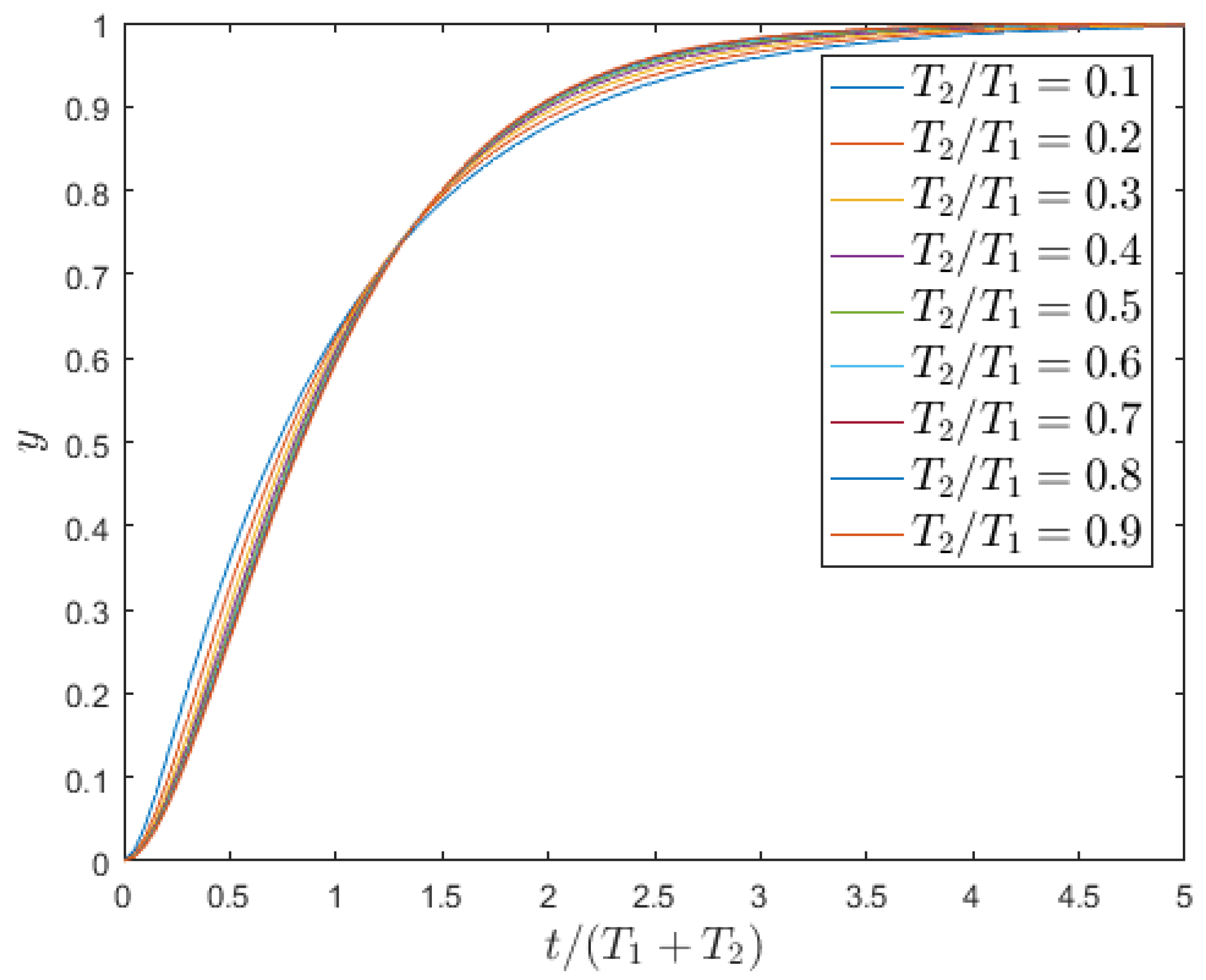
Motivated by this target, we propose a simple but efficient method to describe a heat exchanger system as SOPDT for the purpose of PID parameters tuning. The starting point is trying to approximate the systematic responses before and after identification. By regarding a standard heat exchanger as a SOPDT model, our target is converted to SOPDT model identification. Among all signals adopted for identification, the step response is the most widely applied given its simplicity [22]. 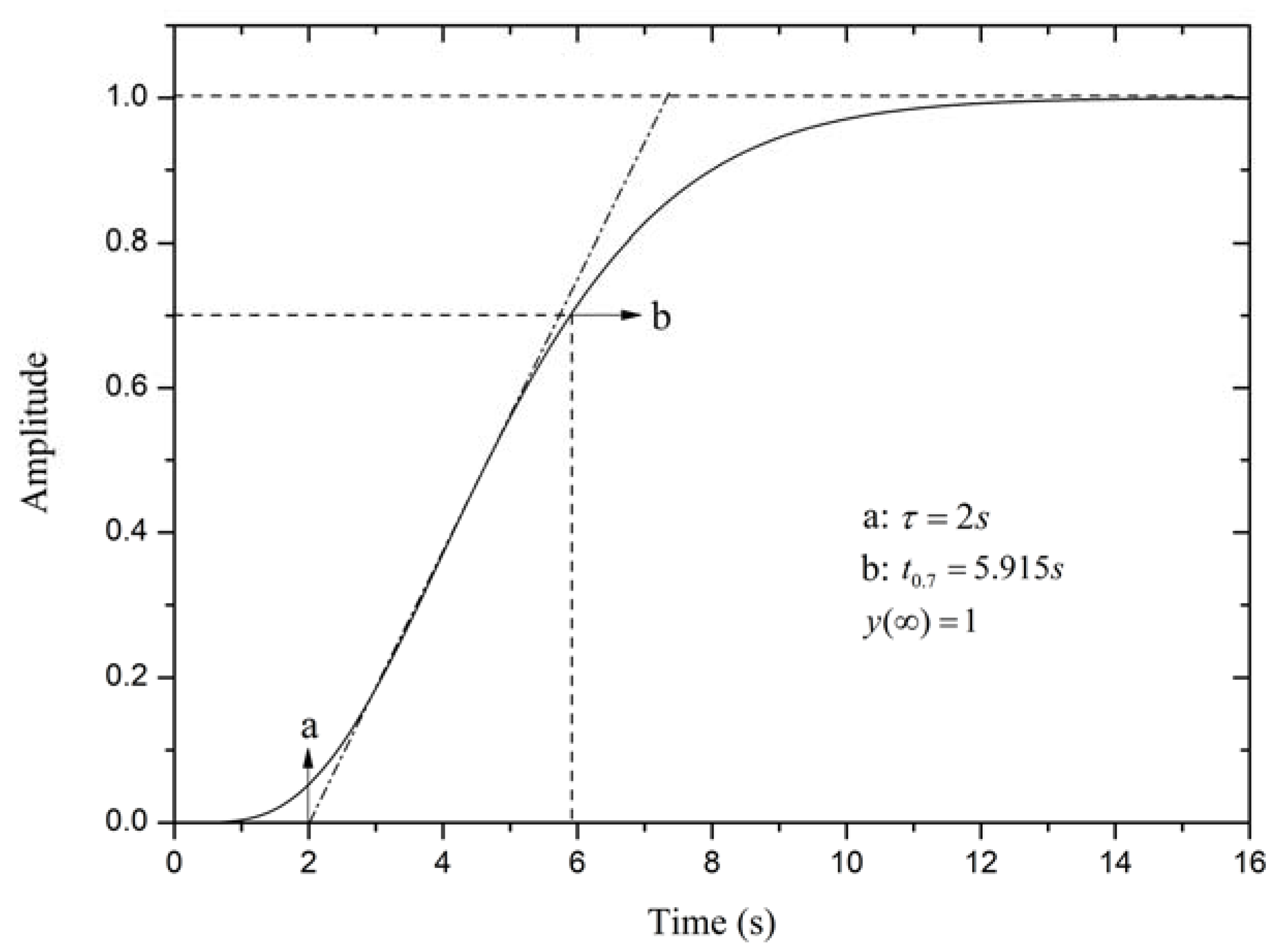The conventional two-point identification method [23,24] can roughly estimate the parameters of SOPDT. However, as shown in Figure 1, the open-loop step responses of general second-order models are converging. Thus, critical points on the open-loop step response curve are illegible. Moreover, high-frequency noise exiting in industry processes unavoidably interferes with information acquisition [25]. Thus, solely relying on the time domain analysis may lead to a low identification precision.

In this paper, a hybrid time and frequency domain method is proposed for heat exchanger identification. A dimensionless time is introduced to simplify the open-loop step response of the SOPDT model. The periodic characteristic of the frequency domain response can reduce error. Compared with traditional identification methods, such as “tangent line” and “two-point” methods, our method shows a higher approximation of the open-loop step response, especially under the existence of noise.

The remainder of the paper is organized as follows: The preliminary results such as the dimensionless step response are given in Section 2. Steps of SOPDT model identification and high-order model reduction are proposed in Section 3. In Section 4, illustrative simulations for identification show the validity of the method. Control simulation of the heat exchanger is given in Section 5. Practical implementation of the real heat exchanger experimental control system confirms the effectiveness of the method in Section 6. The discussion and conclusion parts are given in Section 7 and Section 8, respectively. Appendix A is shown at the end to give some detailed calculation information. All symbols and abbreviations are declared in Appendix B.

2. Preliminary Results

The process model of second-order without delay time is:

$$G(\mathrm{s})=\frac{k_0}{(1+T_{1}s)(1+T_{2}s)}$$

(1)

where $k_0$ is the plant gain, and $T_1$ and $T_2$ are lag constants. For a stable system, $k_0$, $T_1$, and $T_2$ are positive values.

The Laplace transfer of open-loop step response is:

$$Y(\mathrm{s})=\frac{k_0{u}_0}{s(1+T_{1}s)(1+T_{2}s)}$$

(2)

where $u_0$ is the step amplitude. The value of $k_0$ can be determined by the open-loop step response:

$$k_0=\frac{y(\infty )}{u_0}$$

(3)

And a time domain expression of Equation (2) is:

$$y(t)=k_0{u}_0(1-\frac{T_1{e}^{-\frac{t}{T_2}}}{T_1-T_2}+\frac{T_2{e}^{-\frac{t}{T_2}}}{T_1-T_2})=f(t,T_1,T_2)$$

(4)

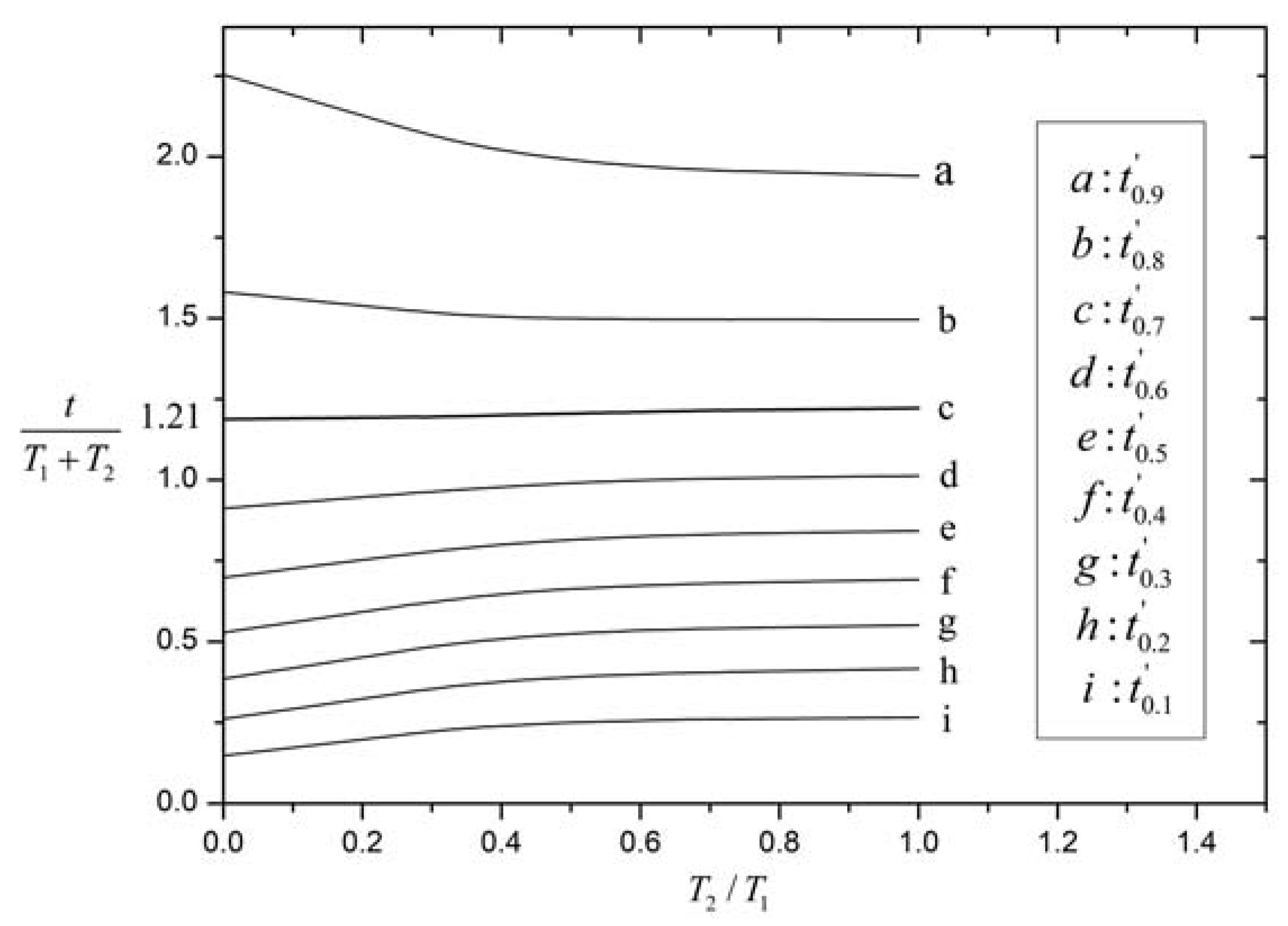
From Equation (4), we see that the open-loop step response is determined by three parameters: $t$, $T_1$, and $T_2$. Motivated by simplifying complicated formula by introducing a dimensionless variable, we apply a dimensionless time variable $t^{\prime }=\frac{t}{T_1+T_2}$. Therefore, a dimensionless expression of the open-loop step response can be derived as:

$$\begin{array}{lll}y(t^{\prime })& =& k_0{u}_0(1-\frac{e^{-\frac{t^{\prime }(T_1+T_2)}{T_1}}}{1-\frac{T_2}{T_1}}+\frac{\frac{T_2}{T_1}{e}^{-\frac{t^{\prime }(T_1+T_2)}{T_2}}}{1-\frac{T_2}{T_1}})\\ & =& k_0{u}_0(1-\frac{e^{-t^{\prime }(1+\frac{T_2}{T_1})}}{1-\frac{T_2}{T_1}}+\frac{\frac{T_2}{T_1}{e}^{-t^{\prime }(1+\frac{T_1}{T_2})}}{1-\frac{T_2}{T_1}})=f(T_2/T_1)\end{array}$$

(5)

Note that the open-loop output $y(t^{\prime })$ merely relies on the value of $T_2/T_1$, rather than $t$, $T_1$ and $T_2$. In other words, when $y(t)$ and $T_2/T_1$ are fixed, $t^{\prime }$ only has a unique value. Therefore, keeping $y(t)$ and $T_1$ as constants, a series of open-loop step response curves are obtained within the increase of $T_2$ from 0 to $T_1$. Meanwhile, the corresponding value of dimensionless time $t^{\prime }$ is derived. Thus, a series of curves can be drawn according to different output amplitudes, as shown in Figure 2.

Figure 2 is denoted as $f(\frac{T_2}{T_1},t_{0.1\times k}^{\prime }),\left(k\in \left[1,9\right]\right)$, where $t_{0.1\times k}$ represents the corresponding time of $0.1\times ky(\infty )$ in $y(t)$. Among nine curves, $f(\frac{T_2}{T_1},t_{0.7}^{\prime })$ is the closest one to a horizontal line. By regarding it as a straight line, we can get an approximation formula:

$$t_{0.7}^{\prime }=\frac{t_{0.7}}{T_1+T_2}=1.21$$

(6)

Consequently, the sum of lag time constants can simply be derived from the formula. Together with a frequency domain analysis presented in the next section, all parameters will be covered. The accuracy and superiority are also given in the following part.

3. Identification and Model Reduction

In this section, simple but accurate procedures for parameter estimation and model reduction are presented.

3.1. Identification of SOPDT Model

A second-order plus delay time (SOPDT) model is the oriented form for complicated system reduction. It is also the starting point that is widely used in controller tuning. However, the prevalently exiting high-frequency noise in the industrial process causes a low identification accuracy, especially the delay time $\tau$. Under this circumstance, we proposed a method based on time and frequency analysis that improves the precision. Particularly, the frequency analysis is mainly based on Nyquist criterion.

The model of second-order with time delay system is:

$$G(\mathrm{s})=\frac{k_0}{(1+T_{1}s)(1+T_{2}s)}{e}^{-\tau s}$$

(7)

where $k_0$ is the plant gain, $T_1$ and $T_2$ are the lag time constants, and $\tau$ is the delay time. The recognition of $k_0$ is the same as Equation (3). We still need three equations of $\tau$, $T_1$, and $T_2$ for solving the problem.

Compared with the second-order without time delay model, the open-loop step response of second-order with time delay actually makes a $\tau$ unit translation toward $t$ axis. Firstly, we get the $\tau$ value by roughly reading the open-loop step response. Then, substitute the estimated value of $\tau$ into Equation (8):

$$T_1+T_2=\frac{t_{0.7}-\tau }{1.21}$$

(8)

where the definition of $t_{0.7}$ is the same as described above. Equation (8) is the first relation of $\tau$, $T_1$, and $T_2$ derived from the open-loop step response.

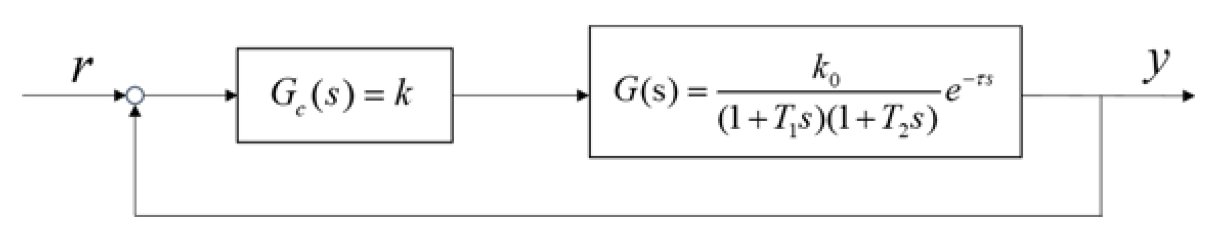
Next, we consider applying Nyquist criterion to the procedure. Therefore, we make a close-loop proportional controlled system, as shown in Figure 3.

$G_c(s)$ is the expression of the proportional controller, $r$ is the input, and $y$ the output. When inputting the unit step signal into the system, the output $y(t)$ changes with different proportional gains $k$. With an exact $k$, output $y(t)$ will exhibit oscillations with an equal amplitude. In this case, the system is under critical circumstance, which means that the open-loop Nyquist curve exactly goes through $(-1,j0)$ on the negative coordinate. Hence, Nyquist criterion works in this situation as Equations (9) and (10),

$$\theta (\omega )=-\left[\tau \omega +\arctan (T_1\omega )+\arctan (T_2\omega )\right]=-\pi$$

(9)

$$M(\omega )=\frac{k_{0}k}{\sqrt{1+T_1^2{\omega }^2}\sqrt{1+T_2^2{\omega }^2}}=1$$

(10)

where $\omega$ is the critical oscillation frequency that can be derived from the oscillation period $T$ with $\omega =\frac{2\pi }{T}$. A simplified expression of Equation (9) is given as Equation (11):

$$\tan (\pi -\tau \omega )=\tan \left[\arctan (T_1\omega )+\arctan (T_2\omega )\right]=\frac{T_1\omega +T_2\omega }{1-T_1{T}_2{\omega }^2}$$

(11)

By substituting $\tau$, $\omega$, and $T_1+T_2$ into Equation (11), we can get the value of $T_1$ and $T_2$ by solving the equation set.

Nevertheless, although all parameters are identified, the value of $\tau$ is too rough. In other words, Equation (10) may not establish. Therefore, we propose an iteration method that is based on the adjustment of $\tau$. The general interval of $\tau$ is limited by solving Equation (11). An empirical rule is: when $T_1$ or $T_2$ is negative, $\tau$ may be far too big. But if $T_1$ or $T_2$ is imaginary, $\tau$ may be too small. After $T_1$ and $T_2$ are all positive numbers, another rule comes when one substitutes the value into Equation (10): if $M(\omega )>1$, reduce $\tau$. Otherwise, increase $\tau$. In a word, during the process, one should strive to make $M(\omega )$ as close to 1 as possible based on established Equations (8) and (9).

3.2. High-Order Model Reduction

Most PID controller tuning methods are based on FOPDT or SOPDT models. However, heat exchangers are prevalently described as high-order models or even more complicated. Thus, developing a convenient and effective reduction method is imperative. The efficiency is evaluated by the original systematic controlled performance, where the controller parameters are tuned based on the reduced model. Also, a high similarity of the open-loop step response and Bode figure before and after reduction indicates a reasonable validity.

Herein, we propose a hybrid reduction method that is mainly aimed at high-order systems. Our starting point is regarding the heat exchanger system as an SOPDT in order to convert the reduction problem into parameter estimation. Therefore, the procedure is almost the same as SOPDT identification. Above all, a proper initial value of $\tau$ is of great importance and will influence the subsequent calculation. We recommend that an appropriate $\tau$ should be near to the systematic delay time, whose definition is the corresponding time to the intersection point of abscissa and tangent line at the inflection point. A detailed example will amply illustrate the steps of system reduction, which is given in Section 4 Part 2.

4. Illustrative Simulation for Identification

Herein, we judge the accuracy by observing how approximate the open-loop step response of the original and identified model is. As the proposed method is noise rejection oriented, we add noise interference to the output pole in the simulation. As we expected, our method shows good robustness, especially under noisy disturbance.

4.1. Example 1. SOPDT with Noise

Consider an example of SOPDT with noise:

$$G_o(s)=\frac{2}{(1+2s)(1+3s)}{e}^{-2.5s}$$

(12)

where the noisy power is 0.001 and sampling time is $0.1s$. We estimate that the delay time $\tau$ is about $2.650s$ and $t_{0.7}=8.589$ by reading the open-loop unit step response of example 1 that is shown in Figure 4. As shown in Figure 5, the critical proportional controller gain $k$ is 1.363, which corresponds to a critical oscillation frequency of $\omega =0.528rad/s$. The final identified results calculated by (8) and (11) and calibrated by (10) are shown below. The detailed calculation process is given in Appendix A.

$$G_i(s)=\frac{2}{(1+1.800s)(1+3.191s)}{e}^{-2.550s}$$

(13)

The open-loop step response of example 1 and identified result are depicted in Figure 6. Two curves almost coincided as one. In order to represent the closeness degree, we introduce the IAE (integral absolute error) index. The IAE value of the two curves is 0.0720, which shows that the proposed method gives a reasonable identified precision and good robustness.

4.2. Example 2. High-Order Model Reduction

Consider a fifth-order system, where:

$$G_o(s)=\frac{1}{{\left(1+s\right)}^5}$$

(14)

Figure 7 shows the unit step response of example 2, where we can precisely obtain the value of $t_{0.7}$ and roughly estimate a systematic delay time $\tau =2s$. Then, we make a proportional controlled close-loop, and adjust the controller gain $k$ until the system exhibits a critical oscillation. The critical state is achieved when $k$ is equal to 2.885 and is depicted in Figure 8. The corresponding frequency is $\omega =0.726rad/s$. The detailed calculation steps are given in Appendix A. Thus, the reduced model is:

$$G_i(s)=\frac{1}{(1+2.053s)(1+1.183s)}{e}^{-2s}$$

(15)

Figure 9 and Figure 10 show the open-loop step response and amplitude-frequency characteristic above −3 dB of the model before and after reduction. A high approximation degree indicates an excellent control performance.

In order to confirm the efficacy of the reduction method, we use a simple controller tuning method proposed by Sigurd [18] to design a PID controller for (14) model and create a single-loop control system like Figure 3. The expression of the PID controller is:

$$G_c(s)=K_c\left(\frac{T_{i}s+1}{T_{i}s}\right)·\left(T_{d}s+1\right)$$

(16)

where $K_c=1.513$, $T_i=2.053$, and $T_d=1.183$, as recommended in [18]. The controlled response under a unit set-point change is depicted in Figure 11. Both models show excellent control quality. Thus, the method is proven to be reasonable and efficient.

5. Control Simulation of Heat Exchanger

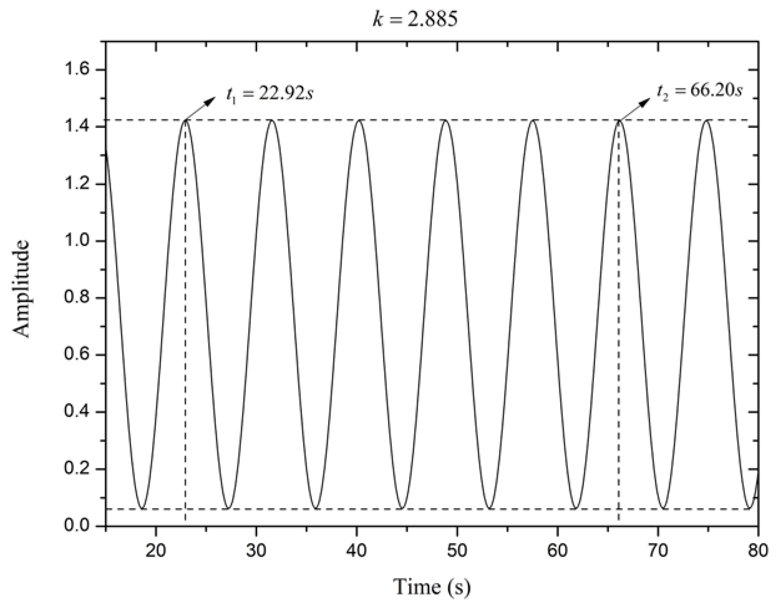
Vasičkaninová and Bakošová [26] introduce a third-order plus delay time model for a heat exchanger, which is represented by:

$$G_o(s)=\frac{5.35\times {10}^4}{{(1+19.5s)}^3}{e}^{-1.5s}$$

(17)

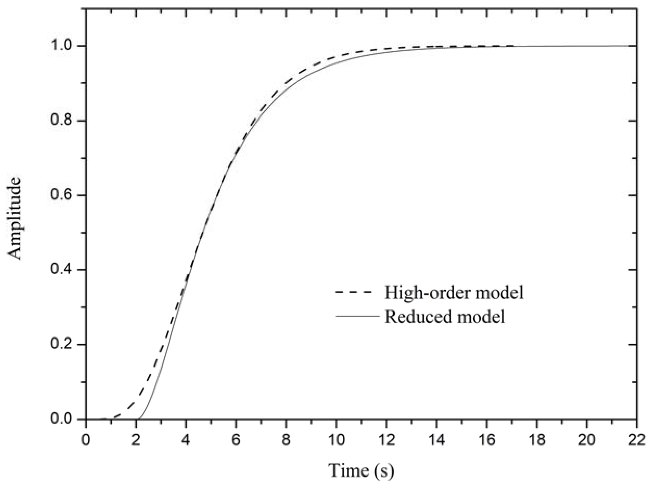
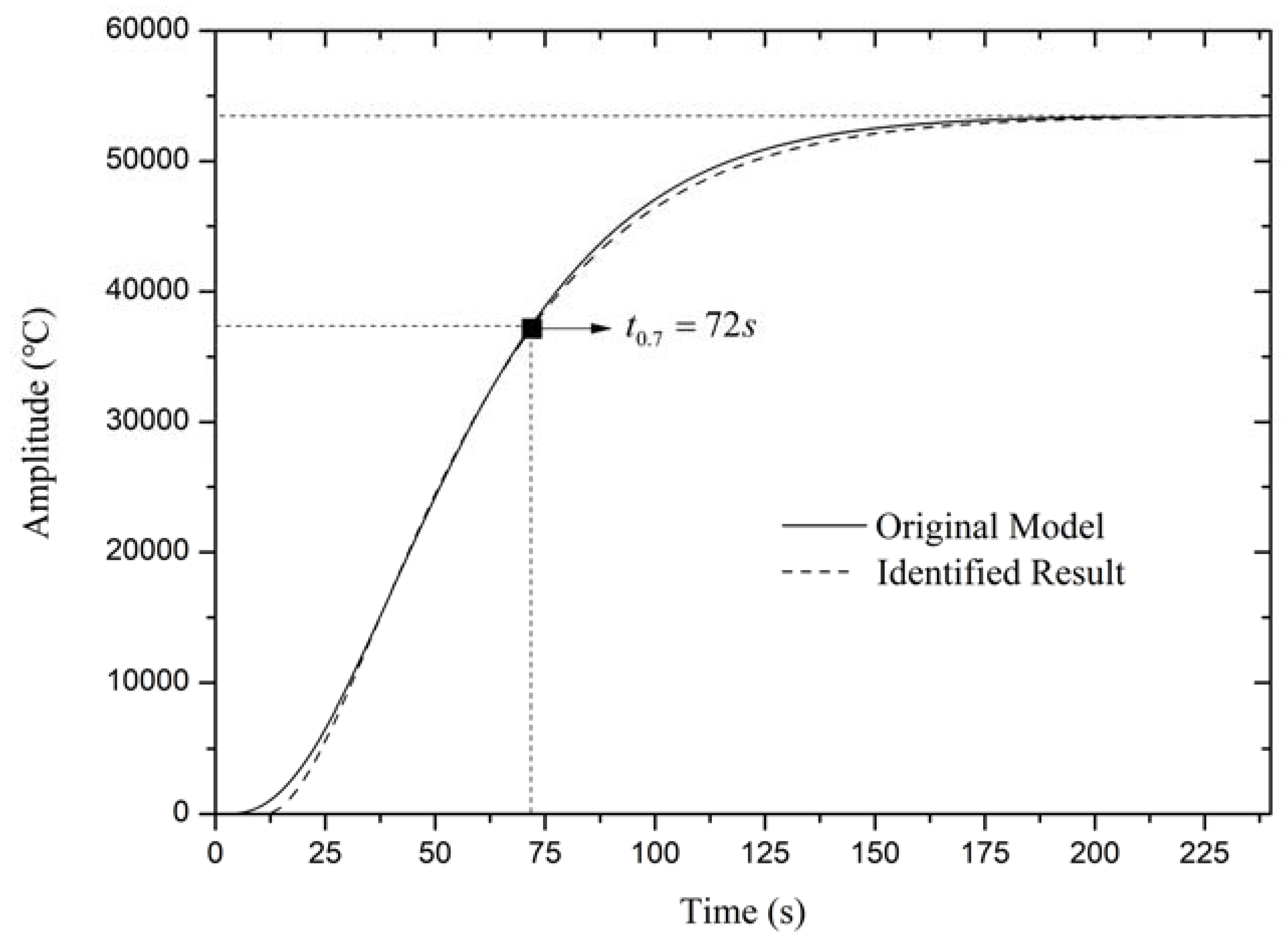
The critical proportional gain that leads to equal-amplitude oscillation is 1.224. The critical oscillation frequency $\omega =0.08101rad/s$ is obtained from Figure 12. The open-loop unit step response is depicted in Figure 13 with a solid line, where we can get $t_{0.7}=72s$ and $\tau =8s$. Thus, the identified SOPDT model for the heat exchanger is:

$$G_i(s)=\frac{5.35\times {10}^4}{(1+25.32s)(1+24.85s)}{e}^{-11.29s}$$

(18)

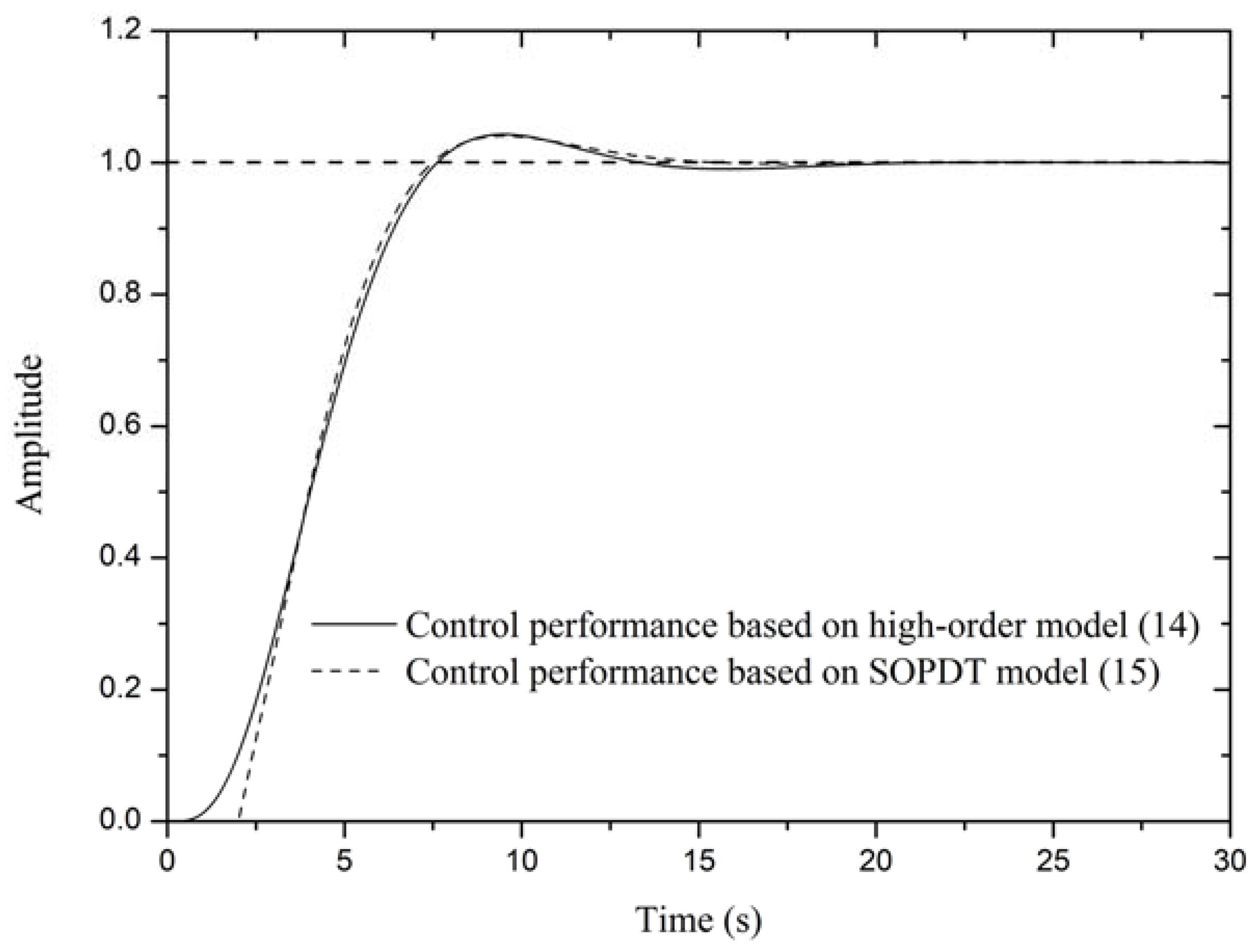
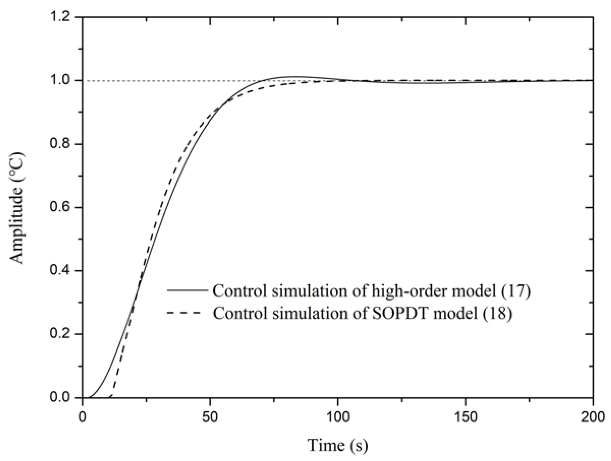
The identified systematic open-loop step response is also shown in Figure 13 with a dashed line. The resemblance of two curves indicates a successful reduction. To further prove the efficacy of the method, the original model is controlled by a PID controller tuned by SIMC [18] based on the reduced model expressed as Equation (18). The control performance is depicted in Figure 14. The original model performs reasonable overshoot and has a short transition period under a step disturbance. The simulation results establish the foundation for the heat exchanger temperature control experiment.

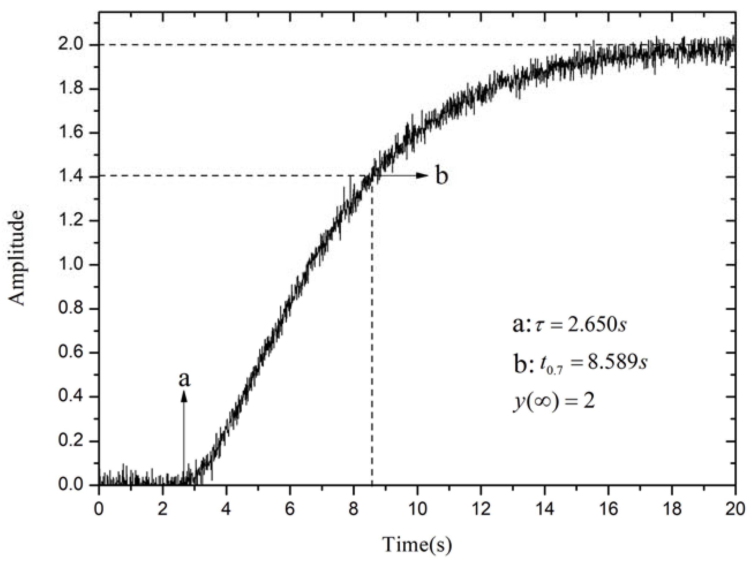
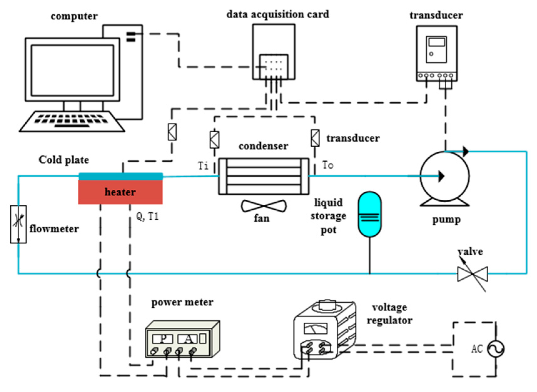
6. Experimental Verification

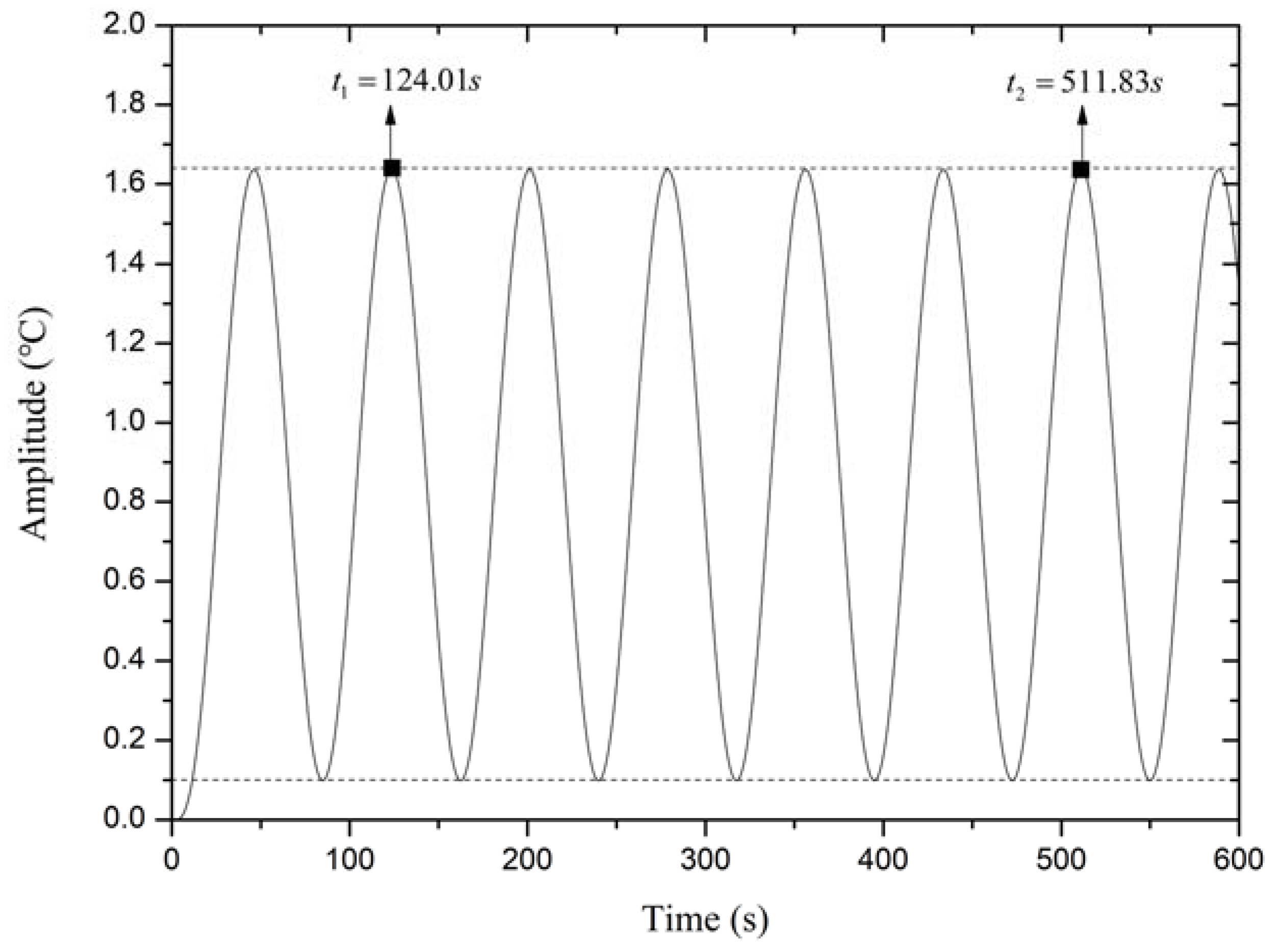
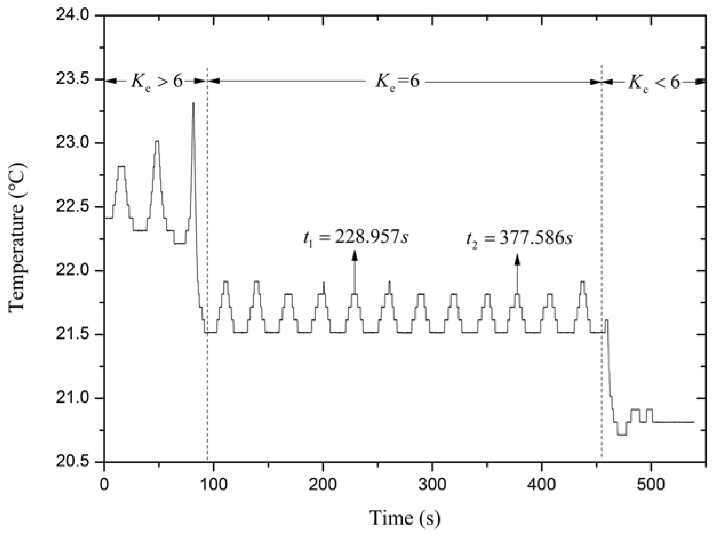
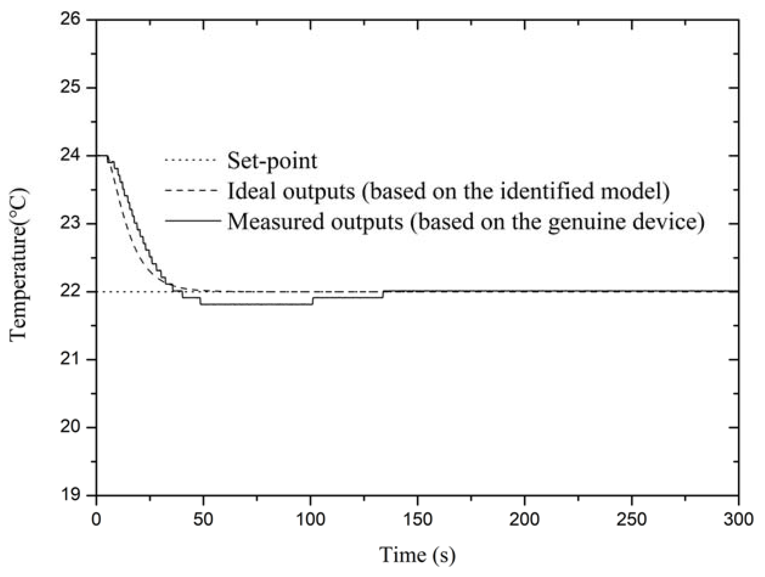
A water-cooling heat exchanger control system is built as shown in Figure 15. The purpose of the experiment is to obtain an ideal temperature control performance by the PID controller, which is tuned based on the identified SOPDT model. According to the proposed method, an open-loop step response and close-loop critical oscillation curves should be provided. 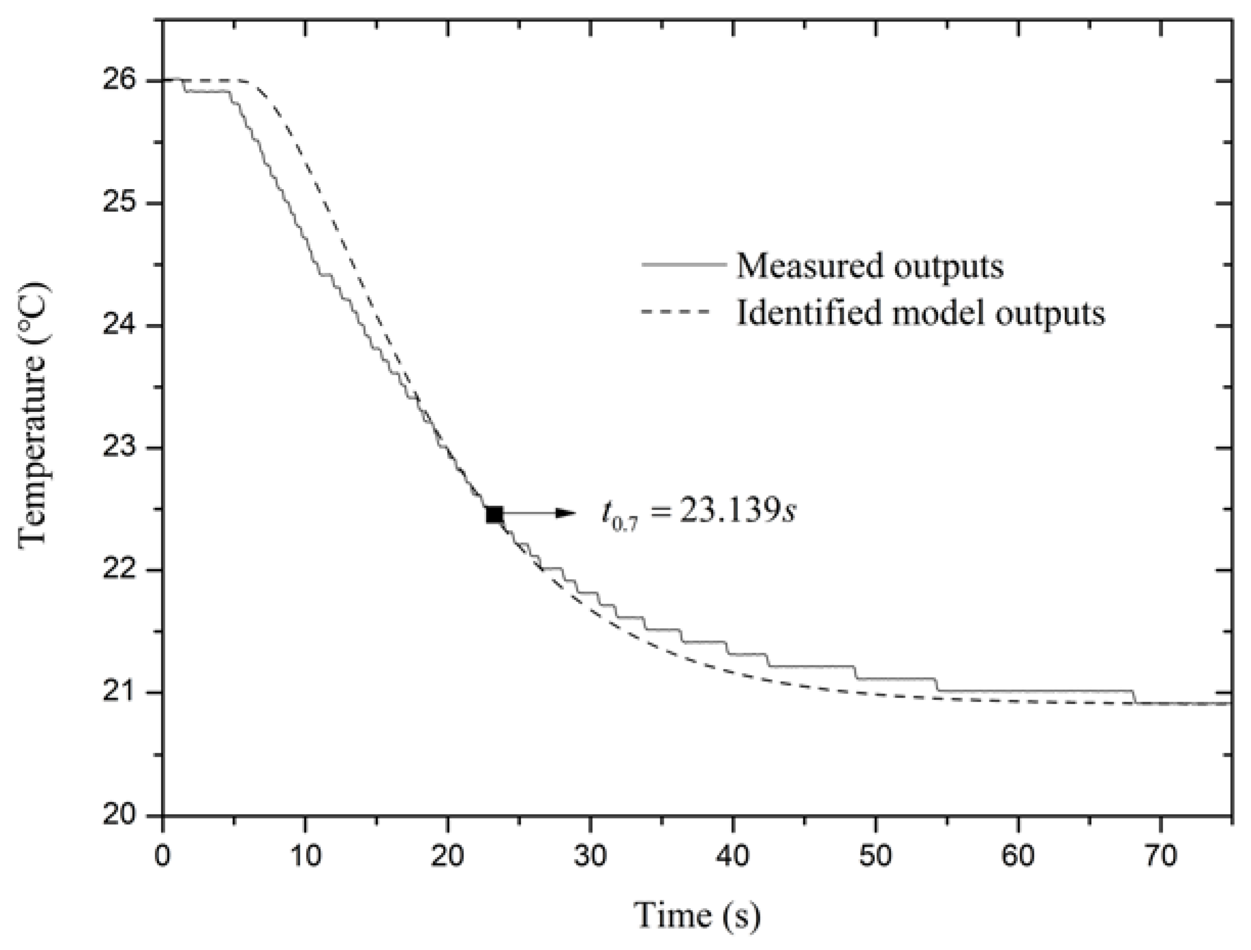Figure 16 is the critical oscillation curve when proportional gain $K_c=6$ under a fixed heating power and fluctuant pumping frequency. 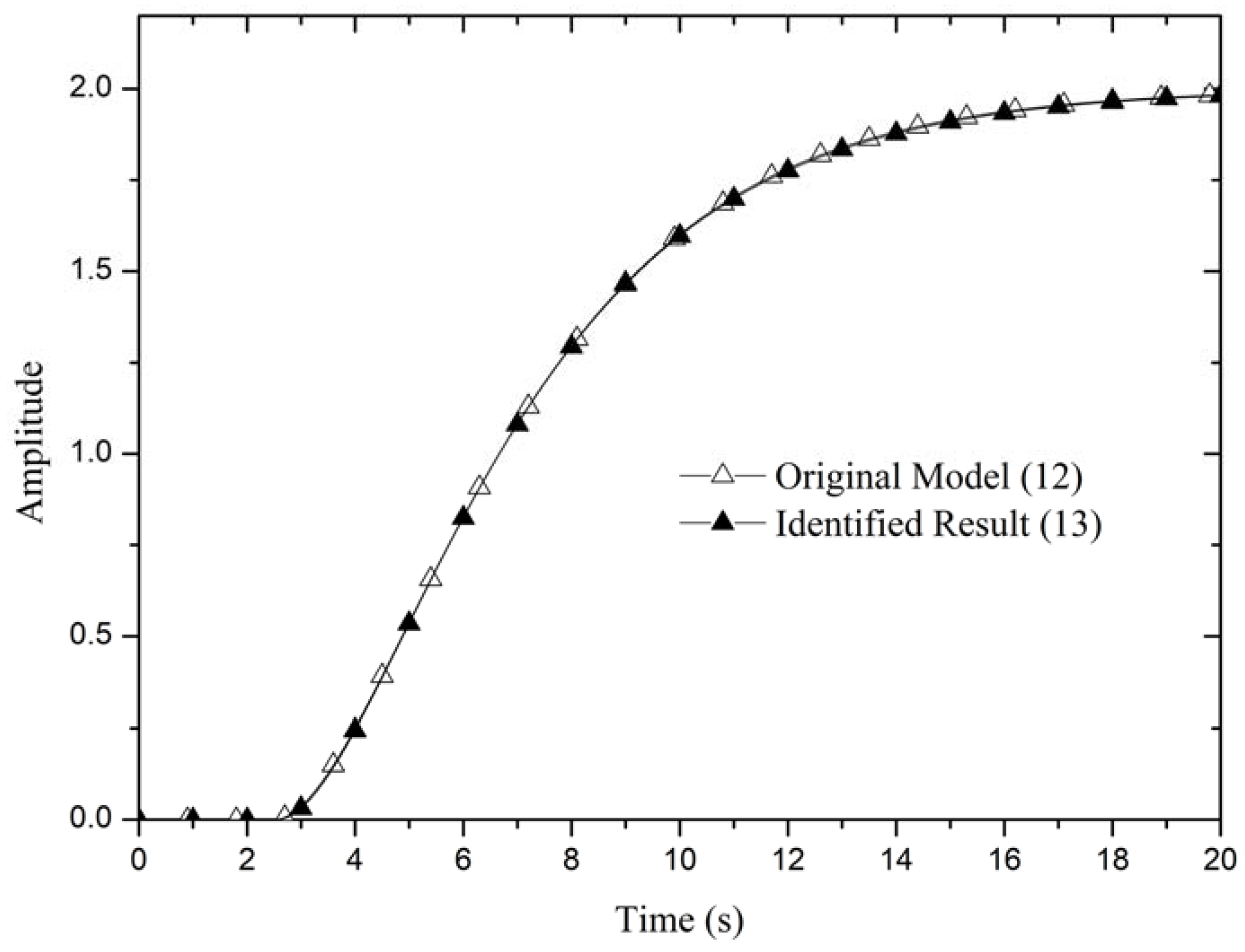The measured open-loop step response of the heat exchanger is given in Figure 17 with a solid line. Based on this, the identified model is expressed as:

$$G_i(s)=\frac{1.700}{(1+7.007s)(1+7.629s)}{e}^{-5.430s}$$

(19)

The open-loop step response of the identified model is also depicted in Figure 17. Two curves in Figure 17 show a high similarity, as we expected. To prove the validity of the reduced model, the PID control performance is shown in Figure 18, while the PID controller parameters are tuned by the SIMC method [18] based on the identified model (19). Figure 18 shows the excellent control quality of the heat exchanger with a short transition period and small overshoot, which confirms the effectiveness of our method. However, the real control process is slightly sluggish compared with the simulation one. The reasons for this include three aspects: an inevitable difference between the original model and reduced model, a stable sampling time of 0.1 s, and a low sensor precision of 0.1 °C.

7. Discussion

Based on the experimental results, the proposed hybrid identification method effectively aids heat exchanger temperature control. The identified model can fully cover the static and dynamic characteristics of the real system. Fully developed PID tuning methods can expediently apply to the reduced models.

The novelty of the method is the combination of time and frequency domain analysis. When excluding the delay time, the proposed method agreed well with the conventional two-point method. Both methods have shown excellent precision. However, the hybrid method is more superior in terms of the delay time and noise disturbance. In addition, the hybrid method is also convenient and feasible for high-order systematic reduction.

The successful implementation on an experimental benchmark heat exchanger confirmed the validity of the method. We also expect a broad application prospect, especially the identification of other similar devices working in sustainable systems. Those model-based PID tuning methods will benefit from the accurate identification and reduction of the hybrid method.

Nevertheless, we absolutely understand its limitation that needs further research. For instance, the first step of the method needs an open-loop step response. However, some systems are never allowed to work without close-loop feedback. The second step requires the system to reach the critical oscillation state, which may be hard to adjust or even cause damage in real production processes. Therefore, our further study will strive to avoid these two problems, but try to work out an ideal identification method that only relies on ordinary close-loop damped oscillation.

8. Conclusions

Aiming at efficient temperature control, this paper proposes a hybrid identification method for the SOPDT model, based on which the SIMC formula is used for PID controller tuning. The identification consists of two steps, respectively, in terms of the step response in the time-domain and the critical point in the frequency domain. By normalizing the step responses of general SOPDT models, a characteristic point is determined as a common intersection, which leads to an equation describing the sum of the lag constants of the SOPDT model. For a complementary purpose, the feedback proportional gain is tuned to produce critical oscillation, from which two more equations can be derived based on Nyquist stability criterion. The time constants and time delay can be readily determined by solving equations. Two examples demonstrate the precision of the identification method, even in the presence of the noise. Moreover, the control simulation based on a benchmark heat exchanger temperature model promises the efficiency of the combination of the identification method and controller tuning. The successful implementation using an experimental system further proves the feasibility of the method, paving a simple but efficient way for heat management in sustainable energy systems.

References

1. Vasičkaninová, A.; Bakošová, M. Control of a heat exchanger using neural network predictive controller combined with auxiliary fuzzy controller. Appl. Therm. Eng. 2015, 89, 1046–1053. [Google Scholar] [CrossRef]
2. Padhee, S. Controller Design for Temperature Control of Heat Exchanger System Simulation Studies. WSEAS Trans. Syst. Control 2014, 9, 485–491. [Google Scholar]
3. Mohanraj, M.; Jayaraj, S.; Muraleedharan, C. Applications of artificial neural networks for thermal analysis of heat exchangers—A review. Int. J. Therm. Sci. 2015, 90, 150–172. [Google Scholar] [CrossRef]
4. Mahitthimahawong, S.; Chotvisut, Y.; Srinophakun, T. Performance comparison of different control strategies for heat exchanger networks. Pol. J. Chem. Technol. 2018, 20, 13–20. [Google Scholar] [CrossRef]
5. Li, D.; Li, C.; Gao, Z.; Jin, Q. On active disturbance rejection in temperature regulation of the proton exchange membrane fuel cells. J. Power Sour. 2015, 283, 452–463. [Google Scholar] [CrossRef]
6. Shan, Y.; Choe, S.-Y. Modeling and simulation of a PEM fuel cell stack considering temperature effects. J. Power Sour. 2006, 158, 274–286. [Google Scholar] [CrossRef]
7. Oravec, J.; Bakošová, M.; Meszaros, A.; Míková, N. Experimental investigation of alternative robust model predictive control of a heat exchanger. Appl. Therm. Eng. 2016, 105, 774–782. [Google Scholar] [CrossRef]
8. Jamal, A.; Syahputra, R. Heat Exchanger Control Based on Artificial Intelligence Approach. Int. J. Appl. Eng. 2016, 11, 9063–9069. [Google Scholar]
9. Sun, L.; Hua, Q.; Shen, J.; Xue, Y.; Li, D.; Lee, K.Y. A Combined Voltage Control Strategy for Fuel Cell. Sustainability 2017, 9, 1517. [Google Scholar] [CrossRef]
10. Sun, L.; Hua, Q.; Shen, J.; Xue, Y.; Li, D.; Lee, K.Y. Multi-objective optimization for advanced superheater steam temperature control in a 300 MW power plant. Appl. Energy 2017, 208, 592–606. [Google Scholar] [CrossRef]
11. Sun, L.; Hua, Q.; Li, D.; Pan, L.; Xue, Y.; Lee, K.Y. Direct energy balance based active disturbance rejection control for coal-fired power plant. ISA Trans. 2017, 70, 486–493. [Google Scholar] [CrossRef] [PubMed]
12. Dormido, S. Advanced PID Control-[Book Review]. IEEE Control Syst. Mag. 2006, 26, 98–101. [Google Scholar] [CrossRef]
13. Lelic, M.; Gajic, Z. A reference guide to PID controllers in the nineties. IFAC Proc. Vol. 2000, 33, 69–78. [Google Scholar] [CrossRef]
14. Alfaro, M.V.; Vilanova, R. Model-reference robust tuning of 2DoF PI controllers for first- and second-order plus dead-time controlled processes. J. Process Control 2012, 22, 359–374. [Google Scholar] [CrossRef]
15. Arif Şen, M.; Tinkir, M.; Kalyoncu, M. Optimisation of a PID controller for a two-floor structure under earthquake excitation based on the bees algorithm. J. Low Freq. Noise Vib. Act. Control 2018, 37, 107–127. [Google Scholar]
16. Santos, D.F.A.; Cismasiu, C.; Bedon, C. Smart glazed cable façade subjected to a blast loading. Struct. Build. 2016, 169, 223–232. [Google Scholar] [CrossRef]
17. Sun, L.; Li, D.; Lee, K.Y. Optimal disturbance rejection for PI controller with constraints on relative delay margin. ISA Trans. 2016, 63, 103–111. [Google Scholar] [CrossRef] [PubMed]
18. Skogestad, S. Simple analytic rules for model reduction and PID controller tuning. J. Process Control 2002, 13, 291–309. [Google Scholar] [CrossRef]
19. Ho, K.W.; Hang, C.C.; Cao, L.S. Tuning of PID controllers based on gain and phase margin specifications. Automatica 1995, 31, 497–502. [Google Scholar] [CrossRef]
20. Albertos, P. Industrial Process Identification and Control Design: Step-Test and Relay-Experiment-Based Methods. IEEE Control Syst. 2014, 34, 78–80. [Google Scholar] [CrossRef]
21. Sung, S.; Lee, J.; Lee, I. Process Identification and PID Control; John Wiley & Sons: Hoboken, NJ, USA, 2009. [Google Scholar]
22. Liu, T.; Wang, Q.-G.; Huang, H.-P. A tutorial review on process identification from step or relay feedback test. J. Process Control 2013, 23, 1597–1623. [Google Scholar] [CrossRef]
23. Rake, H. Step response and frequency response methods. Automatica 1980, 16, 519–526. [Google Scholar] [CrossRef]
24. Marlin, T.E. Process control: Designing processes and control systems for dynamic performance. J. Process Control 2000, 6, 263. [Google Scholar]
25. Segovia, R.V.; Hägglund, T.; Åström, K.J. Measurement noise filtering for PID controllers. J. Process Control 2014, 24, 299–313. [Google Scholar] [CrossRef]
26. Vasičkaninová, A.; Bakošová, M. Robust Control of Heat Exchangers. Chem. Eng. Trans. 2012, 29, 1363–1368. [Google Scholar]
Figure 1. Normalized open-loop step responses of general second-order models.
Sustainability 10 02667 g001
Figure 2. Dimensionless time t with different quotients of time constants.
Sustainability 10 02667 g002
Figure 3. Structure of the close-loop proportional controlled system.
Sustainability 10 02667 g003
Figure 4. Open-loop unit step response of example 1 with noise.
Sustainability 10 02667 g004
Figure 5. Close-loop critical stable response of example 1 when k = 1.363.
Sustainability 10 02667 g005
Figure 6. Open-loop step response of example 1 and the identified result.
Sustainability 10 02667 g006
Figure 7. Open-loop unit step response of example 2.
Sustainability 10 02667 g007
Figure 8. Critical oscillation curves of example 2.
Sustainability 10 02667 g008
Figure 9. Open-loop step response of example 2 before and after reduction.
Sustainability 10 02667 g009
Figure 10. Amplitude-frequency characteristic of example 2 before and after reduction.
Sustainability 10 02667 g010
Figure 11. The control performance of example 2 when input a unit set-point change at t = 0.
Sustainability 10 02667 g011
Figure 12. Critical oscillation of the simulation model.
Sustainability 10 02667 g012
Figure 13. Open-loop step response of the simulation model before and after reduction.
Sustainability 10 02667 g013
Figure 14. Comparison between the control performances of the original model and reduced model.
Sustainability 10 02667 g014
Figure 15. Heat exchanger experimental control facility.
Sustainability 10 02667 g015
Figure 16. Identification experiment to determine the gain parameter of the critical oscillation.
Sustainability 10 02667 g016
Figure 17. Comparison of the open-loop step responses before and after identification.
Sustainability 10 02667 g017
Figure 18. Comparison of the closed-loop PID control performance.
Sustainability 10 02667 g018