Scenario Analysis of Urban Road Transportation Energy Demand and GHG Emissions in China—A Case Study for Chongqing

Abstract

This study, using Chongqing City of China as an example, predicts the future motor vehicle population using the Gompertz Model and the motorcycle population using the piecewise regression model, and predicts and analyzes fuel consumption and greenhouse gas (GHG) emissions of motor vehicles from 2016 to 2035 based on the bottom-up method under different scenarios of improving the fuel economy of conventional vehicles, promoting alternative fuel vehicles, and the mixed policy of the above two policy options. The results indicate that the total population of motor vehicles in Chongqing will increase from 4.61 million in 2015 to 10.15 million in 2035. In the business-as-usual scenario, the road-transportation energy demand in Chongqing will keep increasing from 2015 and will peak in 2030, before it begins to decline by 2035. The trends for the tank to wheel (TTW) and well to wheel (WTW) GHG emissions are similar to that of energy demand. The WTW GHG emissions will increase from 24.9 Mt CO₂e in 2016 to 50.5 Mt CO₂e in 2030 and will then gradually decline to 48.9 Mt CO₂e in 2035. Under the policy scenarios of improving fuel economy of conventional fuel passenger cars, promoting alternative fuel vehicles, and their mixed policy, direct energy consumption and TTW and WTW GHG emissions from 2016 to 2035 will be reduced to different levels. It is also found that the two types of policies have a hedging effect on the direct energy-consumption saving, TTW, and WTW GHG emission reductions. Sensitivity analysis of key parameters and policy settings is conducted to investigate the impact of their changes on the vehicle population projection, direct energy demand, and WTW GHG emissions. Some policy implications are suggested to provide reference for the formulation and adjustment of Chongqing’s, or even China’s, low-carbon road transportation policies in the future based on the analysis results.

1. Introduction

In 2015, the transportation sector accounted for 64.7% of global oil consumption, with road transportation accounting for 49.7% of this [1]. To effectively control the energy consumption and greenhouse gas (GHG) emissions from road transportation, policy makers of nations and cities around the world have developed a series of integrated policy options that include mandatory standards and market-based fiscal policies with economic incentives.

The GHG emission-reduction policies of the road-transportation department can be divided into four types according to the key factors that influence the GHG emissions from vehicles: The vehicle population, fuel economy, fuel type, and kilometers travelled by vehicles (VKT). 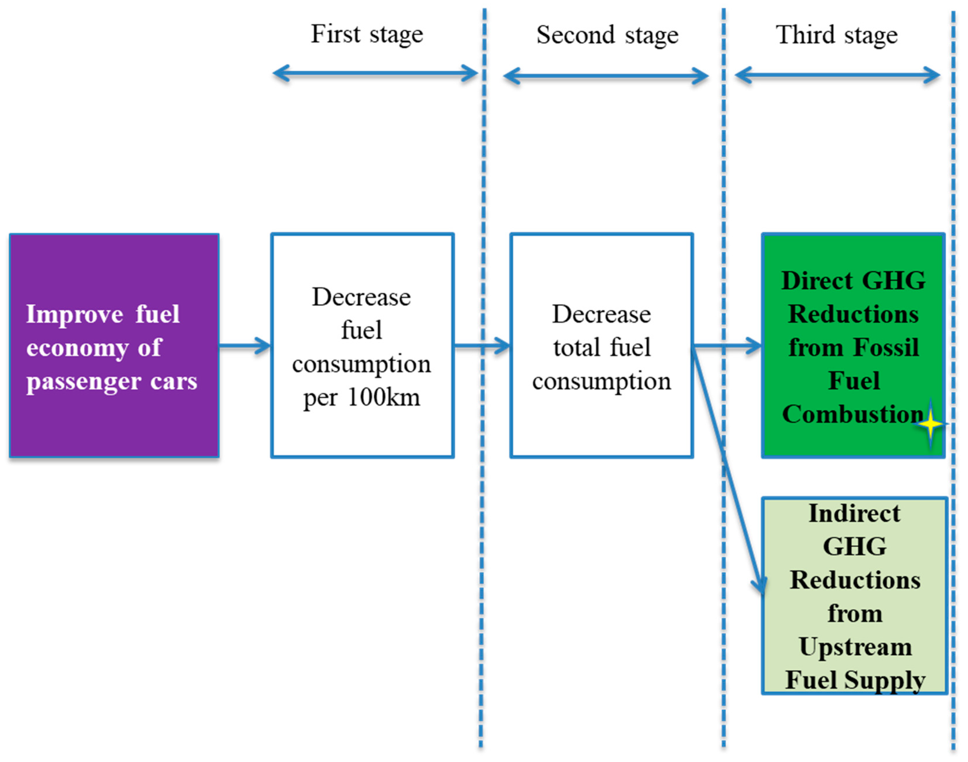The first emission-reduction policy type involves limiting the number of motor vehicles through implementing vehicle purchase taxes [2] and vehicle purchases via a lottery or auction of car license plates [3,4]. 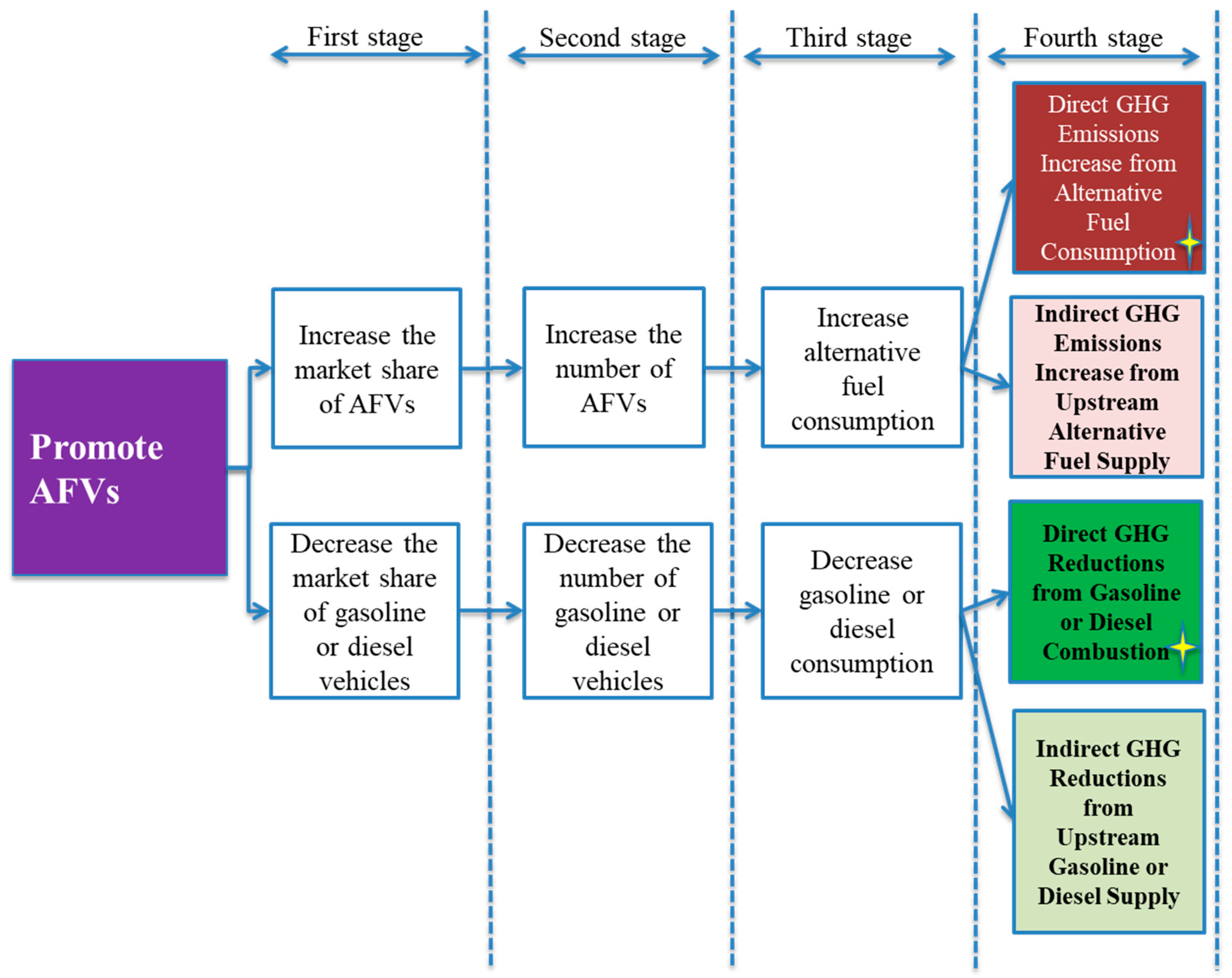The second links to improving the fuel economy of vehicles by, for example, obsoleting cars that do not meet the emission standards set by the government, such as the implementation of the Corporate Average Fuel Economy (CAFE) standards in the USA [5]. The third involves promoting alternative-fuel vehicles (AFVs), such as new-energy vehicles, and this policy can be implemented by, for example, promoting electric vehicles (EVs) [6,7,8], compressed natural-gas (CNG) vehicles, and liquefied natural-gas (LNG) vehicles [9,10]. The last emission-reduction policy aims at controlling the average annual VKT of passenger cars and involves prioritizing the development of public transit systems and restricting vehicle use via plate number and public transport subsidy policies [6,11]. Moreover, some economic policies to reduce vehicle-use intensity (e.g., increasing parking fees and charging congestion fees in urban centers [12,13]) also belong to the fourth type of emission-reduction policy and they have already been implemented in some cities around the world and, yet, are currently only under discussion in China.

The analysis of road-transportation energy demands and GHG emissions, when employing different policy option implementations, has been an important research topic for both domestic and foreign scholars who have established specific models for different regions. Most of the existing studies use bottom-up models to analyze the GHG emission-reduction potential of one or more policy options from among these types of policies.

In terms of the research scope, some studies have undertaken energy-saving and GHG emission-reduction analyses on road-transportation policy options at the international and national levels. At the international level, Hoogwijk et al. [14] employed a bottom-up approach to study the mitigation potential of low-carbon technical policy measures in three world regions (OECD, EIT, non-OECD) by focusing on the policy options related to improving fuel economy and promoting biofuels for motor vehicles. At the national level, Lutsey and Sperling [15] carried out a bottom-up analysis on the key policies related to improving the fuel economy of vehicles and developing hybrid-powered vehicles and low-carbon fuels for the US transport sector. Moreover, Tessum et al. [16] evaluated the impact of GHG emission-reduction policies related to passenger vehicles in the USA on air quality, GHG emission reductions, and human health, with the life cycle theory. Wang et al. [17] used a bottom-up model to estimate the GHG emission-reduction potential of different policy scenarios for China’s road-transportation network, including engine technology improvements, transmission technology improvements, vehicle technology improvements, alternative fuels, and the development of a rapid bus transit system. He et al. [18] predicted gasoline demand and CO₂ emissions by employing different scenarios based on a bottom-up GHG emissions’ accounting model and assessed emission reductions when improving the fuel-economy policy for various types of motor vehicles in China. Yan and Crooks [19] used the long-range energy alternatives planning (LEAP) model to analyze China’s GHG emission-reduction potential when implementing different traffic policies, including controlling the number of private cars (PCs) in use, fuel-economy improvements, developing diesel and natural-gas vehicles, fuel tax, and promoting biofuel use. Besides the policies on improving the fuel economy of vehicles, developing diesel vehicles, and promoting alternative fuels, Huo et al. [20] also analyzed GHG emission reductions in China in terms of the policy of developing EVs and they based their analysis on the bottom-up model. Also, taking China as the research object, Gambhir et al. [10] adopted the previous method [21] and conducted detailed decomposition research on the energy savings and CO₂ emission reductions for each low-carbon vehicle type.

Some other scholars have studied the GHG emission-reduction cost effectiveness of transportation polices at the regional or city level. For example, using detailed data from 48 urban areas in the USA, Hartgen et al. [22] compared CO₂ emission reductions when improving the fuel economy of vehicles, when improving the transportation system, and when shifts in travel behavior took place. Based on this study, Moore et al. [23] evaluated the GHG emission-reduction potential when improving fuel efficiency and signal controls, when reducing vehicle mileage, and when increasing the public transit system’s share. Based on California’s EMFAC2007 (short for EMission FACtor) model, Silva-Send et al. [24] evaluated the GHG emission reductions for seven road-transportation policies developed by local governments in the San Diego County that will come into force by 2020. Zheng et al. [25] and Peng et al. [26] elaborated on the bottom-up method to the provincial level of China. He et al. [27] improved the bottom-up method by adding influencing factors, such as the travel mode, load rate, and the population and per capita travel time to analyze the energy consumption and GHG emission-reduction effects of changes in travel modes brought about through the development of public transport and intelligent city policies.

Besides the bottom-up methods, some scholars take the Life Cycle Assessment (LCA) methods and Greenhouse gases, Regulated Emissions, and Energy use in Transportation (GREET) model to analyze the impact of low-carbon transportation policies. For example, Orsi et al. [28] proposed an exergy-based well-to-wheels (WTW) analysis to compare different passenger vehicles, using the GREET model, based on petroleum energy use, CO₂ emissions, and economic costs in five representative national energy mixes and found no fundamental difference in the fossil fuel pathways among the five nations. Wu et al. [29] analyzed the CO₂ emission-reduction potential of the policy promoting hybrid EVs (HEVs), plug-in HEVs (PHEVs), and pure EVs in three developed regions (Beijing-Tianjin-Hebei, the Yangtze River Delta, and the Pearl River Delta) with the GREET1.8d model combined with a scenario analysis. Zhou et al. [30] used the LCA method to analyze the EV energy consumption and GHG emissions in different grid areas in China and they found significant differences in different regions of China due to different power structures.

There are some weaknesses in the existing literature on road-transportation energy demand and GHG emission analyses under different policy scenarios in China. First, most of the existing studies focus on the national level. As for the studies on the provinces or cities in China, most set the same policy targets when undertaking their scenario analyses for the different regions, making it difficult to reflect the differences arising from the vehicle types and fuel structures in different regions based on the different economic development levels or resource endowments. Some studies fail to consider the energy consumption and GHG emissions from motorcycles, the market share of which is quite large in some cities in China. Second, when analyzing the energy-saving and GHG emission-reduction potential of the various policy options, most studies analyze the impact of a single policy or multiple policies under their own respective policy scenarios and few studies analyze the policy interactions between different policies. Moreover, the analyses of key policy parameters lack sensitivity. In addition, due to the rapid development of China’s new-energy vehicles in recent years, the data and policy targets of the policy analyses need to be updated.

Therefore, based on our previous study [31], this paper takes Chongqing City as an example and uses a bottom-up method, selecting two urban road-transportation low-carbon policies, improving the fuel-economy policy and promoting the development of the AFVs policy, and their mixed policy, to analyze the mechanism of energy savings and GHG emission reductions of the single policy and the mixed-policy. Thus, the main novelty of this paper is that the study incorporates a mixed-policy scenario for urban road-transportation low-carbon policies, based on the causal chain analysis method and the mechanism analysis of energy saving and GHG emission reduction of the single policy and mixed-policy, analyzes the interaction effects of different policies, and compares the evaluation results of the mixed policy with those of the individual policy-implementation scenarios. The cause of the interaction effects from the mixed-policy scenario is then discussed. Thus, the findings from this study can be used in future studies as a reference to help policy makers develop and adjust their low-carbon transportation policies for cities and regions around the world.

This study takes Chongqing City—a city in southwest China—as its case city for two reasons. First, Chongqing is one of the first low-carbon pilot provinces and cities in China, therefore, our findings can act as a low-carbon development reference for similar cities in the southwest. Second, Chongqing City, with its high level of urbanization, is experiencing rapid growth in terms of the number of motor vehicles. This has led to an increasing energy pressure, increasing carbon emissions, and more passenger cars, with PCs accounting for an increasing proportion of urban vehicles. As a result, to achieve low-carbon development, Chongqing needs to urgently undergo a low-carbon transport transformation and upgrading. In this paper, we present two hypotheses: First, in the future, road-transportation policy makers in Chongqing will actively enact low-carbon policies according to the national low-carbon development strategy and plans. Second, we assume that the economy will continue to develop rapidly in the future in Chongqing and that the level of urbanization will continue to improve: These social and economic conditions can support road transportation’s low-carbon transition in Chongqing.

2. Materials and Methods

2.1. Motor Vehicle Types

In this study, by referring to the “China Statistical Yearbook” and “Public Safety Industry Standard on Motor Vehicle Type Terms and Definitions of the People’s Republic of China (GA802-2008),” motor vehicles are divided into three types: Passenger vehicles, trucks, and motorcycles. Passenger vehicles are further divided into heavy-duty buses (HDBs), including urban transit buses and others, medium-duty buses (MDBs), light-duty buses (LDBs), and mini buses. Taxis (TXs) and PCs (LDBs) are listed separately because of their main functions and the differences in their average annual VKTs. Trucks are further divided into heavy (HDTs), medium (MDTs), light (LDTs), and mini trucks, and into two kinds of low-speed trucks (three-wheeled vehicles and low-speed goods vehicles). This specific classification of motor vehicles can be seen in

Table 1. Classification of motor vehicles in this paper.

Category	Type	Function	Abbreviated Code
Buses	Heavy duty	Urban transit	UB
		Others	HDB
	Medium duty		MDB
	Light duty	Taxis	TX
		Private cars	PC
		Others	LDB
	Mini		MiniB
Trucks	Heavy duty		HDT
	Medium duty		MDT
	Light duty		LDT
	Mini		MiniT
	3-wheeled vehicles		3-WT
	Low-speed goods vehicles		4-WT
Motorcycles			MC

below.

2.2. Prediction Model for Vehicle Ownership

The Gompertz model and prediction model from our previous study [31] are used here to predict the total vehicle ownership and the population of each type of vehicles except for motorcycles. The model is as follows:

$$V_t=V^{*}\times {\mathrm{e}}^{\alpha \exp (\beta X_t)}$$

(1)

where X_t represents per capita GDP and functions as the independent variable in this model and V_t represents vehicle ownership per thousand people in the year, t. α and β represent negative parameters to be estimated. V* is the saturation point of vehicle ownership, presuming that V* is a known parameter.

According to Formula (1), combined with the population, P_t, in the year, t, the total motor vehicle population, VP_t, in the year, t, is calculated as follows:

$$V{P}_t=V_t\times P_t/1000$$

(2)

As for the prediction of future motorcycle ownership, according to the related research, when the per capita income of a region reaches a certain amount, the demand for motorcycles will reach its peak after which, with the increase in per capita income, PC ownership will gradually increase. Thus, the demand for motorcycles will tend to fall and motorcycle ownership will decrease gradually [25,32]. Therefore, we use the piecewise regression method and double logarithmic function model based on historical data to predict future motorcycle ownership with Formula (3). The independent variable is the per capita GDP and the dependent variable is motorcycle ownership per thousand people.

$$V_{Mt}=\{\begin{array}{c}{\mathrm{e}}^{{\phi }_1\mathrm{Ln}{X}_t+{\varphi }_1},(X_t\le X_{t*})\\ {\mathrm{e}}^{{\phi }_2\mathrm{Ln}{X}_t+{\varphi }_2},(X_t>X_{t*})\end{array}$$

(3)

where X_t represents per capita GDP and functions as the independent variable in this model and V_Mt represents motorcycle ownership per thousand people in the year, t. φ₁, φ₂, ϕ₁, and ϕ₂ represent parameters to be estimated. t* is the year when motorcycle ownership reaches the peak value, presuming that t* is a known parameter.

As for the market share of each type of vehicle of a certain vehicle age, we presume that the total vehicle population in a given year is the sum of vehicles that have been sold and are still in use. The total vehicle population is calculated using Formula (4). Taking survival rates and the market share of various types of vehicle into account, we use this formula to calculate the ownership of each type of vehicle of a certain vehicle age in each year:

$$V{P}_t={\displaystyle \sum _j{\displaystyle \sum _{k=0}^{{\sigma }_{}}(S_{t-k}\times M_{t-k,j}\times S{R}_{k,j})}}$$

(4)

where σ represents the maximum service life of a vehicle, k represents the age of a vehicle, t − k (t minus k) represents the year that is k years before the year t, VP_t represents the total vehicle population in year, t, S_t−k represents the sales of all types of vehicle in the year t − k, M_t−k,j represents the market share of the type of vehicle, j, in the year t − k, and SR_k,j represents the survival rate (the percentage of cars in use) of the type of vehicle, j, at age, k.

Using this approach, future vehicle sales of each type can be back-calculated based on the projected future total vehicle population in the year, t. The formulae are as follows:

$$S_t=\frac{V{P}_t-{\displaystyle \sum _j{\displaystyle \sum _{k=1}^{{\sigma }_{}}(S_{t-k}\times M_{t-k,j}\times S{R}_{k,j})}}}{{\displaystyle \sum _j(M_{t,j}\times S{R}_{0,j})}}$$

(5)

$$Vtyp{e}_{t,k,j}=S_{t-k}\times M_{t-k,j}\times S{R}_{k,j}$$

(6)

where S_t represents the total sales volume of motor vehicles in the year, t, and ${\displaystyle \sum _j(M_{t,j}\times S{R}_{0,j})}$ is the percentage of newly-sold motor vehicles in the year, t. Vtype_t,k,j represents the vehicle population of the type of motor vehicle, j, with age, k, in the given year, t.

The survival rate in the model is calculated according to the survival-rate curve calculation method [33] using the dual-parameter Weibull distribution as the vehicle survival-ratio function and the vehicle scrap-rate function is defined as the absolute value of the derivative of the vehicle survival-ratio function:

$$S{R}_{t,k,j}=\frac{S{P}_{t,k,j}}{R{P}_{t,j}}=\exp \left(-{(\frac{k}{T_j})}^{W_j}\right)$$

(7)

where SR_t,k,j is the survival rate of type j vehicles that are newly registered in the year, t, at age, k, while SP_t,k,j is the survival number of type j vehicles that are newly registered in the year, t, at age, k. RP_t,j is the total number of newly-sold vehicles of type j registered in the year, t. T_j and W_j are model characteristic parameters. When k = T_j, SR = 1/e, which means the survival rate of vehicles is reduced to 1/e, which is about 36.8%, and T_j is the average age of scrapped vehicles or the average lifetime of type j vehicles.

2.3. Calculation Model for Energy Demand and GHG Emissions

The calculation model for vehicle energy demands and GHG emissions is a bottom-up method and it functions on the basis of establishing an emission list according to vehicle ownership, the VKT, and emission factors per unit of distance. Within a certain area, energy consumption and GHG emissions in a certain year (t) are calculated with the following formula:

$$E_t={\displaystyle \sum _j{E}_{tj}}={\displaystyle \sum _j{\displaystyle \sum _i(}}V{P}_{ijt}\times VK{T}_{ijt}\times F{E}_{ijt}\times Densit{y}_j)$$

(8)

$$GH{G}_t={\displaystyle \sum _{m}GH{G}_{tm}}={\displaystyle \sum _j{\displaystyle \sum _m(E_{tj}\times E{F}_{jm}\times GW{P}_m})}$$

(9)

where i, j, m, and t represent the types of vehicle, types of fuel, type of GHG, and simulated year, respectively. The types of fuel include gasoline, diesel, CNG, electricity, etc. E_t and GHG_t represent, respectively, the road-transport energy consumption (kg) and GHG emissions (g) in the year, t, while VP_ijt, VKT_ijt, and FE_ijt represent the population of type i vehicles that consumes fuel, j, in the year, t, its VKT (km), and fuel economy (L/km), respectively. Density_j represents the density of fuel, j (kg/L), and in this study, the density of gasoline is set at 0.732, with diesel being 0.875. E_tj represents the consumption (kg) of fuel, j, in the year, t. EF_jm represents the emission factors (g kg⁻¹) of the fuel, j, of type m GHG. GWP_m represents the 100-year global warming potential (GWP100) value of type m GHG.

2.4. Mechanism Analysis of Single Policy and Policy Mix

After the implementation of an urban road-transportation low-carbon policy or a mixed-policy, one or more parameters in Formula (8), including VP, VKT, and FE, may change due to the policy effect, resulting in a change of energy consumption and GHG emissions of motor vehicles. In this part, we select improving the fuel-economy policy and promoting the development of the AFVs policy, based on the causal chain analysis method, to give the influence path of energy saving and GHG emission reduction of the two policies and analyze the mechanism of the interaction effect of the mixed-policy.

2.4.1. Improving the Fuel-Economy Policy

Fuel-economy standards are recognized as one of the most effective means by which governments at home and abroad can control motor-vehicle fuel consumption and carbon emissions. The policy object of improving the fuel economy policy of conventional-fuel passenger cars is the fuel economy. The causal chain of the policy is shown in Figure 1. After the implementation of the policy, the fuel economy for the newly-sold conventional-fuel (gasoline, diesel, or CNG) passenger cars is improved every year, which means the fuel consumption rate is reducing every year. Given the situations that other conditions remain unchanged, the total direct fossil fuel consumption consumed by passenger cars will decrease, which reduces the GHG emissions from fuel combustion and the GHG emissions from upstream fuel supply.

2.4.2. Promoting the Development of the AFVs Policy

Since 2005, China has made clear in several related plans and policy options that it will promote the development of new-energy vehicles, especially EVs, to replace traditional vehicles [6]. The policy object of promoting the development of the AFVs policy is the market share of newly-sold alternative fuel vehicles and gasoline or diesel vehicles. The causal chain of the policy is shown in Figure 2. After the implementation of the policy, the market share of some kinds of alternative fuel vehicles in the total newly-sold vehicles will increase. Given the situations that other conditions remain unchanged and the total number of newly-sold vehicles remain unchanged, the number of newly-sold alternative fuel vehicles will increase and the direct alternative fuel consumption, such as natural gas or electricity, will increase, resulting in an increase of GHG emissions from alternative fuel consumption and from the upstream fuel supply. At the same time, with the substitution effect of alternative fuel vehicles to gasoline or diesel vehicles, the number of newly-sold gasoline or diesel vehicles will decrease and the direct gasoline or diesel consumption will decrease, resulting in a decrease of GHG emissions from gasoline or diesel consumption and from the upstream fuel supply. When the absolute value of the change of the total GHG emissions from a decreased gasoline or diesel consumption is larger than that from increased alternative fuel consumption, the direct energy consumptions are saved and total GHG emissions are reduced.

2.4.3. Mechanism Analysis of Policy Mix

The influence path of energy saving and GHG emission reduction from the mixing of the two policies above is, basically, equivalent to the superposition effect of the two policies’ mechanisms, which, that is, simultaneously affect the market share of motor vehicles in different fuel types and the fuel economy of conventional-fuel passenger cars, resulting in the change of the number of newly-sold motor vehicles in different fuel types, with a reduced fuel consumption rate of conventional-fuel passenger cars. Given the situations that other conditions remain unchanged, the direct energy consumptions of different fuels and GHG emissions will change.

However, when the two policies happen to act on the same type of vehicles, an interaction effect of the mixed-policy will occur. Taking the gasoline passenger cars as an example, it is set that, in a certain year, t, without any policy influence, the number of newly-sold gasoline passenger cars is VP_t1. When implementing the single policy of promoting the development of AFVs, the market share of newly-sold electric passenger cars will increase and it is set that the number of newly-sold gasoline passenger cars will decrease by ΔVP_t1 (Policy a). When implementing the single policy of improving the fuel-economy of convention-fuel passenger cars, the fuel consumption rate of a gasoline passenger car will drop by ΔFE_1t (Policy b).

According to Formulas (8) and (9), the energy consumption change caused by ΔVP_t1 from Policy a is as follows:

$$\Delta E^a{}_{t1}=\Delta V{P}_{t1}\times VK{T}_{t1}\times F{E}_{t1}\times Densit{y}_1$$

(10)

The corresponding GHG emission change from Policy a is as follows:

$$\Delta GH{G}^a{}_t={\displaystyle \sum _m(\Delta V{P}_{t1}\times VK{T}_{t1}\times F{E}_{t1}\times Densit{y}_1\times E{F}_{1m}\times GW{P}_m)}$$

(11)

The energy consumption change caused by ΔFE_1t from Policy b is as follows:

$$\Delta E^b{}_{t1}=V{P}_{t1}\times VK{T}_{t1}\times \Delta F{E}_{t1}\times Densit{y}_1$$

(12)

The corresponding GHG emission change from Policy b is as follows:

$$\Delta GH{G}^b{}_t={\displaystyle \sum _m(V{P}_{t1}\times VK{T}_{t1}\times \Delta F{E}_{t1}\times Densit{y}_1\times E{F}_{1m}\times GW{P}_m)}$$

(13)

Under the effect of the mixed-policy of Policy a and Policy b (Policy ab), the market share of the newly sold electric and gasoline passenger cars and the fuel economy of the gasoline passenger cars will be affected simultaneously.

Under the condition that the policies’ enforcement of the mixed-policy is equal to the two policies’ enforcement when implementing alone, respectively, according to Formulas (8) and (9), the energy consumption change caused by ΔVP_t1 and ΔFE_1t from Policy ab is as follows:

$$\Delta E^{ab}{}_{t1}=(\Delta V{P}_{t1}\times F{E}_{t1}+V{P}_{t1}\times \Delta F{E}_{t1}-\Delta V{P}_{t1}\times \Delta F{E}_{t1})\times VK{T}_{t1}\times Densit{y}_1$$

(14)

The corresponding GHG emission change from Policy ab is as follows:

$$\Delta GH{G}^{ab}{}_t={\displaystyle \sum _m\left(\right(\Delta V{P}_{t1}\times F{E}_{t1}+V{P}_{t1}\times \Delta F{E}_{t1}-\Delta V{P}_{t1}\times \Delta F{E}_{t1})\times VK{T}_{t1}\times Densit{y}_1\times E{F}_{1m}\times GW{P}_m)}$$

(15)

From Formulas (10)–(15), we can see that, under the influence of the mixed-policy, there is a reduction amount between the variation of energy consumption, ΔE^ab_t1, and the sum of the variations of energy consumption from the two single policies (ΔE^a_t1 + ΔE^b_t1), which is $(\Delta V{P}_{t1}\times \Delta F{E}_{t1}\times VK{T}_{t1}\times Densit{y}_1)$. This part is the hedging effect from the interaction of these two policies on the energy consumption change. The hedging effect of the corresponding GHG emission change is $(\Delta V{P}_{t1}\times \Delta F{E}_{t1}\times VK{T}_{t1}\times Densit{y}_1\times E{F}_{1m}\times GW{P}_m)$.

2.5. Data Sources and Scenarios Design

2.5.1. GDP and Population Growth

Based on our previous research [31] and a field investigation, we updated the historical data to 2015 and choose 2015 as the new base year. The prediction period is from 2016 to 2035. The historical data for Chongqing’s population and GDP are mainly collected from local statistical yearbooks. The statistics on the future population (2016–2030) are sourced from the local government’s policies and planning document: “Chongqing Population Development Plan (2016–2030).” The population’s growth rate (2031–2035) is taken from the relevant report from the National Development and Reform Commission’s social reform department [34] and from the study [35].

The GDP statistics for 2015–2020 are sourced from the local government’s 13th Five-Year Plan for economic and social development, and the annual growth rate is taken as 9%. From 2021, Chongqing will still be in the middle stage of high-speed development because it is in the western region. According to the related research results on China’s economy, the annual average GDP growth rate in Chongqing will be 7% from 2020–2025, 6% from 2025–2030, and 5% from 2030–2035. In this paper, the GDP data are calculated as a constant-price GDP in 2010. Chongqing’s future population growth rate and average annual growth rate per capita GDP are shown in

Table 2. Chongqing’s future population and per capita GDP annual growth rate.

Year	2015–2020	2020–2025	2025–2030	2030–2035
Resident population growth	1.19%	1.22%	1.15	0.34%
Per capita GDP growth	7.72%	5.71%	4.80%	4.65%

.

2.5.2. Vehicle Population

The historical vehicle-population data for 1990–2015 and motorcycle-population data for 1996–2015 are gathered from Chongqing’s statistical yearbooks and data on the fuel structure are from development reports and planning documents for the transportation sector in Chongqing. According to the field investigation and the collation of the literature, statistical yearbooks, and statistical data, the fuel types of the motor vehicles in Chongqing mainly include gasoline, diesel, CNGs, LNGs, HEVs, PHEVs, and pure EVs. The vehicle-ownership saturation point in Chongqing is still set to 250 cars per 1000 people according to our previous research [31].

The future market share of various motor-vehicle types in Chongqing is set as follows. First, the market share of motorcycles is determined according to the forecast results of the piecewise regression model. Then, in terms of the market share for each type of automobile from 2016–2035, the vehicle-ownership data for Chongqing from 2005–2015 shows that, due to the development of HDVs and LDVs, the proportion of MDVs exhibited a significant downward trend. Due to the mountain terrain in Chongqing, mini vehicles exhibited a significant downward trend. The PC ownership proportion increased steadily and the proportion of all buses (except for PCs) and all trucks showed a steady downward trend. Therefore, according to the trends in the above analysis, and by referring to Wang et al. [17] for the forecast of the motor-vehicle market share in China, we set the proportion of all kinds of automobiles in

Table 3. 2015, 2020, 2025, and 2035 automobiles market share (%).

Automobile Type	2015 (present)	2020	2025	2035
HDT	3.51	2.47	1.95	1.82
MDT	1.21	0.85	0.67	0.63
LDT	8.59	6.04	4.77	4.45
MiniT	0.00	0.00	0.00	0.00
HDB	0.71	0.63	0.62	0.58
UB	0.41	0.48	0.47	0.44
MDB	0.47	0.49	0.49	0.46
LDB	37.41	38.11	37.69	35.21
MiniB	0.36	0.37	0.37	0.35
TX	0.84	0.87	0.86	0.81
PC	45.86	49.50	52.04	55.25
3-WT	0.02	0.01	0.01	0.01
4-WT	0.61	0.17	0.05	0.01
Total	100	100	100	100

, and the proportion of other years for each period is calculated via linear interpolation.

Referring to the relevant research results of [36,37], the vehicle age-distribution data of various types of motor vehicle are shown in

Table A1. Age distribution of various types of vehicles in 2015.

Vehicle Age	LDB, MiniB, PC	LDT, MiniT, 3-WT, 4-WT	MDB	MDT	HDB, HDT	UB	TX	MC
1	18.5%	17.8%	20.0%	19.8%	18.0%	22.0%	14.5%	13.6%
2	29.4%	28.3%	22.0%	21.4%	24.0%	31.0%	35.4%	18.1%
3	15.9%	15.4%	18.0%	17.6%	16.0%	16.0%	37.2%	11.5%
4	15.4%	14.8%	11.0%	10.8%	13.0%	15.0%	9.3%	18.6%
5	10.3%	11.2%	10.0%	11.0%	12.0%	8.0%	3.0%	15.5%
6	6.5%	7.4%	9.0%	9.4%	7.0%	5.0%	0.6%	13.5%
7	2.3%	2.5%	7.0%	7.2%	6.0%	1.2%	0.6%	8.8%
8	1.4%	1.6%	1.6%	1.8%	2.4%	1.0%		0.2%
9	0.2%	0.6%	1.0%	0.8%	1.3%	0.7%		0.1%
10	0.1%	0.4%	0.4%	0.2%	0.3%	0.1%		0.1%

. The W_j parameter in Formula (6) of the model and the vehicle’s average lifetime are from the parameter regression results of study [33] and they have been adjusted to be in line with China’s compulsory scrapping standards for motor vehicles, as shown in

Table A2. Model parameters of the model of motor vehicle survival.

Vehicle Type	Average Lifetime (Years)	Wj
HDB	15	5.33
UB	13	∞
MDB	15	5.33
LDB	10	5.33
TX	8	∞
PC	15	4.79
MiniB	10	4.79
HDT	15	5.58
MDT	15	5.58
LDT	15	5.58
MiniT	12	5.58
MC	13	4.79
3-WT	9	5.58
4-WT	12	5.58

.

2.5.3. Average Annual Vehicle Kilometers Traveled

The ideal annual average mileage of motor vehicles (VKT) should be collected through the I/M (Inspection Maintenance Program) system and be updated yearly [38]. However, at present, officials neither report nor publish the VKT data for motor vehicles in China’s different cities. Therefore, the base VKT yearly data for all kinds of motor vehicles in Chongqing mainly come from related studies by Chongqing scholars [37] and from the annual report on traffic development in Chongqing in 2015. As for the future VKT data, according to the research by [25], heavy-duty vehicle VKT (HDBs and HDTs) will increase gradually and VKTs of LDBs and motorcycles will decline gradually. Therefore, we set the VKTs of HDBs and HDTs to increase by 0.50% every year and the VKTs of LDBs and motorcycles to decrease by 0.50% every year from 2016–2035. As PCs are mostly used for commuting between home and work, we set the VKT of PCs to remain unchanged at the 2015 level and it is assumed that the VKTs of other types of vehicle will also remain unchanged at the 2015 level. The VKT data in this study are shown in

Table 4. VKT of motor vehicles.

VKT (1000 km/vehicle)	2015	2020	2025	2030	2035
HDT	45	47	48	49	50
MDT	28	28	28	28	28
LDT	32	32	32	32	32
MiniT	38	38	38	38	38
HDB	83	85	87	89	92
UB	83	85	87	83	92
MDB	28	28	28	28	28
LDB	29	27	26	24	23
MiniB	34	34	34	34	34
TX	179	179	179	179	179
PC	18	18	18	18	18
MC	8	8	7	6	6
3-WT	21	21	21	21	21
4-WT	28	28	28	28	28

as follows:

2.5.4. Scenario Design for Fuel Economy

The fuel economy of a vehicle (kilometers travelled per unit of energy use) is a key parameter to determine on-road vehicle GHG emissions [39]. The fuel-economy data of various types of motor vehicles in Chongqing are difficult to obtain, but many scholars have undertaken studies on the fuel economy of China’s motor vehicles. Therefore, data for the fuel economy of vehicles in China prior to 2010 are sourced from the research of Argonne National Laboratory (ANL) [40] and Huo et al. [41], with reference to the first to the third stages of the Fuel-Economy Standards of China. The fuel-economy data prior to 2010 are assumed to remain unchanged. The fuel-economy data from 2011 to 2015 are based on the published data by the Ministry of Industry and Information.

As for the fuel-economy data for 2016–2035, we set up two scenarios: The natural change scenario (FE0) and the policy-implementation scenario whereby the fuel economy of conventional-fuel passenger cars improves (FE1).

In the FE0 scenario, according to both home and overseas studies, even without any mandatory requirements, the motor-vehicle fuel consumption per kilometer will gradually decrease because of the improvements in vehicle technology in the automobile manufacturing industry. For example, the American scholars, Davis et al. [42], found that the fuel economy of cars and light trucks in the USA improved by 0.47% to 0.53% every year from 1990–2009 without any policy requirements being in place and, according to the vehicle inventory surveys conducted by the US Census Bureau, it was found that, despite no new fuel-economy requirements, the fuel economy of the US HDTs improved by about 1% every year from 1977 to 2002 [43]. Therefore, in this paper, it is assumed that from 2015 to 2035 the fuel-consumption rate of heavy- and medium-duty vehicles for gasoline, diesel, and natural gas in Chongqing will improve by 1% per year and the fuel-consumption rate of light-duty vehicles will improve by 0.5% per year. In

Table A3. Fuel consumption rate in 2010 and 2015 and the data in 2020, 2025, and 2035 under the FE0 scenario (unit: L/100 km).

Vehicle Type	Fuel Type	2010	2015	2020	2025	2030	2035
HDT	Diesel	24.90	23.70	22.55	21.46	20.41	19.42
	LNG	19.34	19.34	18.40	17.51	16.66	15.85
MDT	Gasoline	21.08	20.06	19.09	18.16	17.28	16.44
	Diesel	16.87	16.05	15.27	14.53	13.82	13.15
LDT	Gasoline	10.00	9.75	9.51	9.28	9.05	8.83
	Diesel	11.90	11.61	11.32	11.04	10.77	10.50
	EV	1.67	1.67	1.67	1.67	1.67	1.67
MiniT	Gasoline	10.00	9.75	9.51	9.28	9.05	8.83
	Diesel	11.90	11.61	11.32	11.04	10.77	10.50
HDB	Gasoline	27.58	26.24	24.96	23.75	22.60	21.50
	Diesel	22.06	20.99	19.97	19.00	18.08	17.20
	LNG	17.13	17.13	16.30	15.51	14.75	14.04
UB	Gasoline	27.58	26.24	24.96	23.75	22.60	21.50
	Diesel	22.06	20.99	19.97	19.00	18.08	17.20
	CNG	30.10	28.33	26.96	25.65	24.40	23.22
	PHEV	15.88	15.88	15.11	14.37	13.68	13.01
	EV	12.13	12.13	11.54	10.98	10.45	9.94
MDB	Gasoline	22.27	22.27	21.19	20.16	19.18	18.25
	Diesel	17.81	17.81	16.95	16.13	15.34	14.60
	CNG	25.58	25.58	25.58	25.58	25.58	25.58
LDB	Gasoline	7.80	7.04	6.87	6.70	6.53	6.37
	Diesel	6.24	5.63	5.49	5.36	5.23	5.10
	CNG	6.30	6.30	6.14	5.99	5.85	5.70
	HEV	4.00	4.00	4.00	4.00	4.00	4.00
	EV	1.67	1.67	1.63	1.59	1.55	1.51
MiniB	Gasoline	7.80	7.04	6.87	6.70	6.53	6.37
PC	Gasoline	7.80	7.04	6.87	6.70	6.53	6.37
	CNG	6.30	6.30	6.14	5.99	5.85	5.70
	HEV	5.00	5.00	5.00	5.00	5.00	5.00
	PHEV	4.00	4.00	4.00	4.00	4.00	4.00
	EV	1.45	1.45	1.41	1.38	1.34	1.31
TX	Gasoline	7.80	7.04	6.87	6.70	6.53	6.37
	CNG	6.30	6.30	6.14	5.99	5.85	5.70
MC	Gasoline	2.50	2.50	2.50	2.50	2.50	2.50
3-WT	Diesel	3.73	3.73	3.73	3.73	3.73	3.73
4-WT	Diesel	8.67	8.67	8.67	8.67	8.67	8.67

, we list the fuel-consumption rate data for different types of vehicle and fuel in 2010 and 2015, and the data for 2020, 2025, and 2035 are based on the FE0 scenario.

Besides gasoline and diesel, the fuel-economy unit or the fuel-consumption rate of other fuels such as CNG, LNG, HEVs, PHEVs, and EVs is calculated and converted to L/100 km according to the calorific values of gasoline or diesel. For example, the fuel-consumption rate (kwh/100 km) for EVs is sourced from the energy-saving and new-energy vehicle technical roadmap published in 2017 [44] and, in 2015, the average electricity-consumption rate of electric PCs in China was 13 kwh/100 km. According to the energy-conversion coefficient, every thousand liters of gasoline equals to 0.03235 TJ, therefore, the electricity-consumption rate of electric PCs converted to the gasoline-consumption rate is 1.45 L/100 km. The conversion herein is only made to enable a comparison of the fuel economy and direct energy consumption for differently fueled vehicles, while for the calculation of GHG emissions, the emission factors (kgCO₂e/TJ) of different fuels are still adopted. As for PHEVs, according to the literature [10], it is set so that 75% of the total vehicle kilometers travelled by PHEVs comes from conventional fuels, such as gasoline, diesel, or LNG, while 25% comes from electricity consumption. Therefore, the fuel-consumption rate of a PHEV is the sum of 75% of the fuel-consumption rate of the gasoline, diesel, or LNG vehicle type and 25% of the fuel-consumption rate of the EV type. In Chongqing, there are PHEV urban buses (UBs) powered by LNG and electric UBs and PHEV PCs powered by gasoline and electricity.

In the FE1 scenario, it is assumed that China will, in the future, strengthen the implementation of its fuel-economy policy for conventional-fuel passenger cars. The standard for improving the fuel economy of conventional-fuel passenger cars in Chongqing is the same as for China as a whole. According to the energy-saving and new-energy vehicle technical roadmap published in 2017 [44], we set the average fuel-consumption rate for newly-sold conventional gasoline passenger cars and for CNG passenger cars at 5.7 L/100 km and 5.1 L/100 km up to 2020, 5.2 L/100 km and 4.6 L/100 km up to 2025, 4.8 L/100 km and 4.3 L/100 km up to 2030, and 4.5 L/100 km and 4 L/100 km up to 2035.

2.5.5. Scenario Design for Alternative Fuel Vehicles

Except for EVs, some other AFV technologies, such as LNG and CNG, have already been implemented in taxis, buses, and some PCs in Chongqing. For the AFV market share (e.g., NGVs, PHEVs, EVs, and others) in Chongqing for 2016–2035, this study also sets up two scenarios: The natural change scenario (AFV0) and a policy scenario of vigorously promoting AFVs (AFV1).

For the AVF0 scenario, we set the fuel structure in Chongqing for 2016–2020 to maintain the 2011–2015 trend, with no new strengthening policy to change the motor-vehicle fuel structure, while the fuel structure for 2021–2035 remains unchanged at the 2020 level.

For the AVF1 scenario, according to the Chongqing Municipal People’s Government’s suggestions on accelerating the application of new-energy vehicles, by 2020, there will be 100,000 EVs (including PHEVs) in Chongqing and, in 2015, Chongqing officially unbanned the “oil-modified gas” of non-operating vehicles and began to promote the modification and sales of CNG PCs. According to the 2015–2030 promotion targets in the policy documents for PHEVs, EVs, CNG, and LNG vehicles, such as the Notice on Improving the Subsidy Policy for Urban Buses’ Refined-oil Prices and Speeding Up the Popularization and Application of New-energy Vehicles, and Suggestions on the Promotion and Application of LNG Vehicles (Ships) in Chongqing, we set the policy targets for the AFV1 scenario, and the fuel shares for the newly-sold HDTs, HDBs, UBs, LDBs, PCs, and LDTs in Chongqing for 2016–2035 are listed in

Table A4. Fuel market share of newly sold vehicles by vehicle type in Chongqing.

Vehicle Type	Fuel Type	2015	AF0				AF1
			2020	2025	2030	2035	2020	2025	2030	2035
HDB	Gasoline	15.3%	15.3%	15.3%	15.3%	15.3%	15.3%	15.3%	15.3%	15.3%
	Diesel	83.4%	83.3%	83.3%	83.3%	83.3%	74.2%	73.8%	73.8%	73.8%
	LNG	1.3%	1.4%	1.4%	1.4%	1.4%	10.5%	11.0%	11.0%	11.0%
UB	Gasoline	0.1%	0.1%	0.1%	0.1%	0.1%	0.1%	0.1%	0.1%	0.1%
	Diesel	4.0%	3.8%	3.8%	3.8%	3.8%	3.8%	3.8%	3.8%	3.8%
	CNG	75.5%	71.7%	71.7%	71.7%	71.7%	66.1%	61.1%	56.1%	46.1%
	PHEV	17.6%	21.1%	21.1%	21.1%	21.1%	26.0%	30.3%	34.7%	43.3%
	EV	2.8%	3.3%	3.3%	3.3%	3.3%	4.0%	4.7%	5.3%	6.7%
MDB	Gasoline	28.9%	29.5%	29.5%	29.5%	29.5%	29.5%	29.5%	29.5%	29.5%
	Diesel	36.2%	35.0%	35.0%	35.0%	35.0%	35.0%	35.0%	35.0%	35.0%
	CNG	34.9%	35.6%	35.6%	35.6%	35.6%	35.6%	35.6%	35.6%	35.6%
LDB	Gasoline	95.8%	95.8%	95.8%	95.8%	95.8%	90.0%	82.0%	57.0%	47.0%
	Diesel	1.9%	1.9%	1.9%	1.9%	1.9%	1.9%	1.9%	1.9%	1.9%
	CNG	1.2%	1.2%	1.2%	1.2%	1.2%	1.2%	1.2%	1.2%	1.2%
	HEV	0.01%	0.01%	0.01%	0.01%	0.01%	0.01%	0.01%	0.01%	0.01%
	EV	1.2%	1.2%	1.2%	1.2%	1.2%	7.0%	15.0%	40.0%	50.0%
PC	Gasoline	97.7%	97.7%	97.7%	97.7%	97.7%	90.0%	79.0%	52.0%	41.0%
	CNG	2.0%	2.0%	2.0%	2.0%	2.0%	3.0%	6.0%	8.0%	9.0%
	HEV	0.03%	0.03%	0.03%	0.03%	0.03%	0.03%	0.03%	0.03%	0.03%
	PHEV	0.001%	0.001%	0.001%	0.001%	0.001%	0.001%	0.001%	0.001%	0.001%
	EV	0.3%	0.3%	0.3%	0.3%	0.3%	7.0%	15.0%	40.0%	50.0%
TX	Gasoline	2.9%	2.9%	2.9%	2.9%	2.9%	2.9%	2.9%	2.9%	2.9%
	CNG	97.1%	97.1%	97.1%	97.1%	97.1%	97.1%	97.1%	97.1%	97.1%
MiniB	Gasoline	100%	100%	100%	100%	100%	100%	100%	100%	100%
HDT	Diesel	99.0%	98.9%	98.9%	98.9%	98.9%	57.7%	57.7%	57.7%	57.7%
	LNG	1.0%	1.2%	1.2%	1.2%	1.2%	42.3%	42.3%	42.3%	42.3%
MDT	Gasoline	3.1%	3.3%	3.3%	3.3%	3.3%	3.3%	3.3%	3.3%	3.3%
	Diesel	96.9%	96.7%	96.7%	96.7%	96.7%	96.7%	96.7%	96.7%	96.7%
LDT	Gasoline	32.3%	36.0%	36.0%	36.0%	36.0%	36.0%	36.0%	36.0%	36.0%
	Diesel	64.0%	60.2%	60.2%	60.2%	60.2%	57.0%	49.0%	24.0%	14.0%
	EV	3.7%	3.8%	3.8%	3.8%	3.8%	7.0%	15.0%	40.0%	50.0%
MC	Gasoline	100%	100%	100%	100%	100%	100%	100%	100%	100%
3-W RV	Diesel	100%	100%	100%	100%	100%	100%	100%	100%	100%
4-W RV	Diesel	100%	100%	100%	100%	100%	100%	100%	100%	100%

.

2.5.6. Scenario Design for Policy Mix

According to the policy-scenario designs for improving the fuel-economy policy and promoting the development of the AFV policy, the following four scenarios were set up: The business-as-usual (BAU) scenario, the policy scenario of individually implementing improvements in the fuel-economy policy for conventional-fuel passenger cars (IFE), the policy scenario of individually implementing the policy for promoting AFVs (PAFV), and the mixed-policy scenario combining the implementation of the two categories of policies (PM). The combination pattern of the four scenarios is shown in

Table 5. The combination pattern of the four scenarios.

		Fuel Economy Improvement
		No	Yes
AFV promotion	No	BAU	IFE
	Yes	PAVF	PM

as follows.

2.5.7. GHG Emission Factors

Data regarding GHG emission factors (except for electricity) are also based on our previous study and are supplemented by published reports by the civil government on VKTs in Chongqing in 2015. Therefore, the vehicle GHG emissions in this study also consist of two parts. One part of the emissions comes from fuel use, the tank-to-wheel (TTW) process, which is also referred to as downstream GHG emissions. The other part of the emissions is from extraction and distribution, or from well to tank (WTT), which is also referred to as upstream GHG emissions. This part also includes GHG emissions from the generation of electric power, which means that, according to the WTT emission factor, the GHG emissions generated by EV and PHEV power consumption can be accounted for. Together, the upstream and downstream stages combine to form the life cycle of GHG emissions from vehicle fuel use or from well to wheel (WTW) [45]. Therefore, GHG emission factors from different types of vehicle fuel consumption also consist of an upstream and downstream stage. Moreover, we adjusted the emission factors of different vehicle fuels based on the latest research from China [46]. The 100-year global warming potential (GWP100) values for CO₂, CH₄, and N₂O are decided based on the IPCC Fifth Assessment Report [47], which are 1, 34, and 298, respectively.

With regards to the electric-power emission factor, it is assumed that it will continue to decrease due to the continuous optimization of China’s energy structure in the future. By referring to the 13th Five-Year Plan for Chongqing’s electric-power production and research by the China Energy Research Association [48], as shown in

Table 6. Predictions for the future power-supply structure of the Central China Power Grid.

	2015 (Present)	2020	2025	2030	2035
Coal-fired	64%	54%	50%	47%	39%
Hydroelectric	30%	28%	26%	25%	23%
Gas-fired	5%	13%	17%	20%	24%
Wind	1%	2%	3%	3%	4%
Other	0%	3%	4%	5%	10%

, we list the predictions for the future power-supply structure of the Central China Power Grid for Chongqing. The main bases are as follows: First, the coal-fired power ratio will fall due to the low-carbon development trend of Chinese power generation and the lower future coal-fired power subsidies. Second, there will be a slight decrease in the proportion of hydropower because the hydropower resource in Chongqing is limited and, although the total amount will increase in the future, the proportion will reduce. Third, the proportion of natural-gas electricity will increase, which is caused by the lower international market price of natural gas due to the US shale-gas revolution. As the market price of natural gas decreases, imports of natural gas will increase and, along with the development of the Belt and Road construction, imports of natural gas from Burma, Kazakhstan, Russia, and other countries will increase. Moreover, the shale-gas reserves in Chongqing are rich and, with future technological breakthroughs, the mining of gas will greatly increase. Although most of the natural gas will be transferred to areas outside of Chongqing, some will still be left for local use and so the proportion of natural-gas power generation will increase. Lastly, other energy resources, such as wind energy and solar energy, will also increase, but the growth rate is limited, mainly because Chongqing belongs to the fourth type of wind-energy resource area designated by the National Development and Reform Commission and these resources are relatively insufficient compared with other regions. At the same time, because of the fog in Chongqing, solar resources are insufficient.

The emission factors of the different fuel types are shown in

Table A5. Downstream and upstream GHG emission factors of vehicle fuels.

	Downstream GHG Emissions			Upstream GHG Emissions
	CO2	CH4	N2O	GHG
Unit	kgCO2/TJ	kgCH4/TJ	kgN2O/TJ	tCO2e/TJ
Gasoline	67,914	3.8	5.7	17.8
Diesel	72,585	3.9	3.9	17.7
CNG	55,539	92	3.0	25.2
LNG	55,612	92	3.0	25.2
HEV	67,914	3.8	5.7	17.8

and

Table A6. GHG emission factors for electricity.

	Unit	2010	2015	2020	2025	2030	2035
Electricity	kgCO2e/TJ	218,957	192,165	178,790	171,648	159,608	141,073

.

3. Results

3.1. Vehicle Population Projection

In this study, the Gompertz model is used to predict the number of motor vehicles (except for motorcycles). By using the least-squares parameter estimation and a model simulation, the prediction model for motor-vehicle ownership in Chongqing is obtained as follows:

$$V_t=250\times {\mathrm{e}}^{-4.61\times \exp (-0.33X_t)},\left(R^2=0.983\right)$$

(16)

As for the prediction model for motorcycles, we carried out a piecewise regression analysis of the data on motorcycle ownership (V_Mt) and per capita GDP (X_t) in Chongqing from 1996–2015 (the related data are shown in

Table A7. Data for model regression.

	Population (10,000 People)	Per Capita GDP (Yuan/Person)	Motorcycle Population (10,000 Units)	Vehicle Population (Except for Motorcycle) (10,000 Units)
1990	2920.90	2704.20	-	6.3
1991	2938.99	2935.22	-	7.2
1992	2950.78	3405.95	-	9.3
1993	2964.92	3918.18	-	10.5
1994	2985.59	4415.87	-	13.2
1995	3001.77	4932.55	-	13.5
1996	2875.30	5736.14	6.14	15.72
1997	2873.36	6382.99	7.06	17.39
1998	2870.75	6938.67	11.21	16.60
1999	2860.37	7506.53	14.19	18.84
2000	2848.82	8192.66	17.43	21.13
2001	2829.21	9008.88	19.32	25.47
2002	2814.83	10,005.16	26.94	29.07
2003	2803.19	11,221.98	36.34	34.25
2004	2793.32	12,657.70	42.88	34.84
2005	2798.00	14,114.88	58.87	51.22
2006	2808.00	15,808.37	70.95	60.39
2007	2816.00	18,269.42	76.16	67.32
2008	2839.00	20,749.17	84.15	76.91
2009	2859.00	23,673.51	106.90	94.15
2010	2884.62	27,475.30	155.14	117.56
2011	2919.00	31,604.21	204.43	129.95
2012	2945.00	35,585.52	226.60	159.57
2013	2970.00	39,626.60	211.11	192.93
2014	2991.40	43,631.19	200.23	237.17
2015	3016.55	48,026.56	179.71	278.97

). According to the results of the regression, before 2012, motorcycle ownership per thousand people in Chongqing increased with the growth in per capita GDP and, after 2012, motorcycle ownership per thousand people decreased slowly with the growth in the per capita GDP. The prediction model for the ownership of motorcycles is obtained as follows:

$$V_{Mt}=\{\begin{array}{c}{\mathrm{e}}^{1.9179\mathrm{Ln}{X}_t-15.557},(X_t\le X_{2012})(R^2=0.974)\\ {\mathrm{e}}^{-0.756\mathrm{Ln}{X}_t+12.267},(X_t>X_{2012})(R^2=0.976)\end{array}$$

(17)

Based on the above equations, we estimate the motor-vehicle population and growth in Chongqing from 2016 to 2035, with our findings shown in Figure 3 below. Comparing the forecasted data for 2016 and 2017 with the actual data, as shown in

Table 7. Test on prediction of vehicle population in 2016 and 2017.

Unit: 10,000	2015	2016				2017
	Base period	Actual data	Prediction	Error		Actual data	Prediction	Error
				(1 year gap)	(5 years gap)			(1 year gap)	(5 years gap)
Vehicle population	461.38	510.25	511.35	0.22%	4.38%	567.50	562.69	−0.85%	3.12%

, the absolute error value for each year is below 1%, and, if a time gap of five years was used to do the regression and to predict 2016 and 2017 vehicle ownership based on values of per capita GDP and vehicle ownership data during 1990–2012, we found that the 2016 error was 4.38% and the 2017 error was 3.12%. Therefore, the prediction, generally, matches the actual data. According to the forecasted results, the total number of motor vehicles will increase from 4.61 million in 2015 to 10.10 million in 2030 and reach saturation point at 10.15 million in 2035. The number of motor vehicles (except for motorcycles) will increase from 2.87 million in 2015 to 8.92 million in 2030 and will reach 9.14 million in 2035. The rapid increase in the vehicle population can be attributed to the growth potential of PCs and LDBs. The proportion of PCs in Chongqing will rank first in the future. Regarding the types of motor vehicle, with the decline in motorcycles and the increase in PCs, by 2017, the PC population (1.81 million) will exceed motorcycles (1.79 million) and will remain in first place from 2017–2035, accounting for 28.0~49.8% of all motor vehicles from 2015 to 2035. The PC population will increase about three times from 1.29 million in 2015 to 5.05 million in 2035. Followed by PCs, the population of LDBs, which are the cars used for businesses and companies, account for 22.8% in 2015, increasing to 31.7% in 2035.

We also estimate the total vehicle kilometers travelled for the different vehicle types in Chongqing from 2016 to 2035, as shown in Figure 4. According to the results, the total number of vehicle kilometers travelled will increase from 102.7 million thousand km in 2016 to 220.7 million thousand km in 2030 and will decrease to 218.5 million thousand km in 2035. In the short term, from 2016 to 2021, the vehicle types with the most total vehicle kilometers travelled will be LDBs, PCs, and motorcycles, and the total vehicle kilometers travelled by PCs will be 1.9 times that of motorcycles in 2016. In the medium and long term, with the change in the number of motor vehicles, the total vehicle kilometers travelled will exceed motorcycles from 2022 onwards. From 2027, the total vehicle kilometers travelled by PCs will exceed LDBs and will rank first. By 2035, with the increasing PC mileage, the total vehicle kilometers travelled by PCs will be 16.3 times that of motorcycles.

3.2. Direct Energy Demand

Figure 5, Figure 6 and Figure 7 present the total direct energy demands of the road-transportation sector in Chongqing up to 2035 under different scenarios. In the BAU scenario, the total vehicle direct energy demand will keep increasing from 2015 to reach its peak in 2030 at about 576,437 TJ and then it will begin to decline to 559,411 TJ by 2035.

In the IFE scenario, as Figure 5 shows, by improving the fuel economy of conventional passenger cars, the total vehicle direct energy demand will peak in 2029, one year earlier than that in the BAU scenario, and the energy-consumption peak will be 492,012 TJ, which is 14.6% less than the peak value in the BAU scenario. With regards to the energy-consumption structure, the main vehicle fuels under the BAU and IFE scenarios are gasoline, diesel, and CNG, with slight changes in their proportions from 2016 to 2035. In the IFE scenario, the proportion of petroleum (gasoline and diesel) consumption is expected to fall from 91.7% to 89.0% from 2016 to 2035 and is the most important fuel for vehicles in Chongqing. Natural-gas vehicles (including CNG and LNG vehicles) will increase gradually and the proportion is predicted to account for between 8.0% and 10.3% of the total fuel consumption from 2016 to 2035. With the trend in promoting new-energy vehicles from 2010 in Chongqing, the power-consumption ratio of EVs will increase slightly from 0.3% in 2016 to 0.8% in 2035. To sum up, in the BAU and IFE scenarios, most vehicle fuel consumption in Chongqing will still be based on traditional oil-based fuels and the development of natural gas will make good progress, but the proportion of EVs will still be very small.

In the PAFV scenario, as Figure 6 shows, vehicles equipped with various alternative-fuel technologies with higher energy efficiencies than conventional gasoline and diesel vehicles (including EVs, PHEVs, CNG, and LNG vehicles) will gradually diffuse into the market. The total vehicle direct energy demand will peak in 2027, three years earlier than in the BAU scenario, and the energy-consumption peak will be 519,143 TJ, which is 9.9% less than the peak value in the BAU scenario. As vehicle energy sources become more diversified and alternative fuels play a more important role than in the BAU scenario, the energy-consumption structure will change up to 2035, with gasoline at 52.7%, diesel at 20.2%, CNG at 13.4%, LNG at 5.5%, PHEVs at 0.9%, and EVs at 7.4%. The proportion of petroleum (gasoline and diesel) consumption is expected to fall from 91.7% to 72.3% from 2016 to 2035, which is a significant decrease compared with that in the BAU and IFE scenarios.

In the PM scenario, as Figure 7 shows, under the joint action of improving the fuel economy of conventional passenger cars and promoting AFVs, the total vehicle direct energy demand will peak in 2026, four years earlier than in the BAU scenario. The energy-consumption peak will be 459,734 TJ, which is 20.2% less than the peak value in the BAU scenario and is the lowest peak value among all four scenarios. The energy-consumption structure will change up to 2035, with gasoline at 47.6%, diesel at 23.5%, CNG at 12.9%, LNG at 6.4%, PHEVs at 1.0%, and EVs at 8.7%.

According to the summary of the calculation results, the cumulative changes in direct energy consumption from 2016–2035 for the IFE, PAFV, and PM scenarios compared to the BAU scenario are shown in Figure 8. The savings in direct energy consumption in the diagram are shown in a columnar chart and the total net energy saving is presented as a red point. A negative value indicates an increase in energy consumption for some type of fuel in a policy scenario. Under these three scenarios, energy-saving effects take place. Regarding the cumulative total energy saving, from 2016–2035, the PM scenario has the largest energy saving, reaching 1.7 million TJ. The energy savings of the IFE and PAFV scenarios will be 1.1 million TJ and 0.8 million TJ, respectively.

It is notable that, in the case of the mixed policy, the total energy saving from 2016–2035 is 0.2 million TJ less than the sum of the energy savings from the two single-policy scenarios; that is, the two policies produce a hedging effect on direct energy consumption. The cause of the hedging effect is through the implementation of the policy promoting EVs and natural-gas vehicles as the share of EVs and CNG cars among the PCs will increase and the share of conventional gasoline cars will reduce, which will indirectly reduce the fuel-consumption savings caused by the separate implementations for improving the fuel economy via the conventional-fuel passenger car policy.

As for the type of fuel consumption, as

Table 8. Cumulative direct energy saving ratio for policy scenarios compared to the BAU scenario during 2016–2035.

	IFE	PAFV	PM
Gasoline	15.3%	14.7%	26.5%
Diesel	0.3%	18.6%	18.9%
CNG	9.8%	−3.7%	7.9%
LNG	0.0%	−1804.4%	−1804.4%
HEV	0.0%	0.0%	0.0%
PHEV	0.0%	−31.7%	−31.7%
Electricity	0.0%	−1099.5%	−1099.5%
Total energy saving	10.9%	8.5%	17.3%

Note: A negative number indicates the incremental fuel consumption.

shows, compared with the BAU scenario, from 2016–2035, the cumulative direct energy consumption of gasoline, diesel, and CNG will decrease by 15.3%, 0.3%, and 9.8%, respectively, under the IFE scenario. The cumulative direct energy consumption of gasoline and diesel will decrease by 14.7% and 18.6%, respectively, under the PAFV scenario, but, due to the increasing share of AFVs, the cumulative direct energy consumption of CNG and LNG vehicles, PHEVs, and EVs will increase by 3.7%, 1804.4%, 31.7%, and 1099.5%, respectively. The energy-saving effects of gasoline and diesel in the PM scenario were the largest and they will decrease by 26.5% and 18.9%, respectively, while CNG cars will decrease by only 7.9%. The cumulative direct energy-saving effects of gasoline and diesel in the PM scenario are the largest and they will reduce by 26.5% and 18.9%, respectively, and CNG cars will reduce by 7.9%. However, the energy consumption of LNG vehicles, PHEVs, and EVs will increase by 1804.4%, 31.7%, and 1099.5%, respectively. It can be further found that the hedging effect of the two types of policies that we analyzed is mainly reflected in the impact on gasoline and CNG cars, which happen to be the objects to be influenced by the two types of policies.

3.3. GHG Emissions

From the two accounting prospects of TTW and WTW GHG emissions, this part analyzes the emission-reduction potential of GHG emissions in Chongqing from 2016–2035 under the different scenarios. The TTW GHG emissions for Chongqing’s road transportation from 2016–2035 for the BAU scenario and the policy scenarios are shown in Figure A1, Figure A2 and Figure A3, where the overall trend for the TTW GHG emissions of vehicles in Chongqing is similar to that of the direct energy demand. The detailed results for the TTW GHG emissions are shown in Appendix A.

The WTW GHG emissions in Chongqing for road transportation from 2016–2035 for the BAU scenario and the policy scenarios are shown in Figure 9. In the BAU scenario, the WTW GHG emissions will increase from 24.9 Mt CO₂e in 2016 to 50.5 Mt CO₂e in 2030 and will then gradually decline to 48.9 Mt CO₂e in 2035. Compared to the BAU scenario, in the IFE scenario, the WTW GHG emissions will reduce by 4.0%, 14.6%, and 17.4% in 2020, 2030, and 2035, respectively. The increase in the GHG emission-reduction proportion is mainly due to the gradual replacement of old cars with new high fuel-economy vehicles. Newly-added passenger cars will produce cumulative emission reductions in the later period following policy implementation. The difference between the WTW GHG emission-reduction ratio and the TTW GHG emission-reduction ratio is very small for each year and WTW GHG emissions will peak in 2029. However, compared to the BAU scenario, the reduction effect is not so obvious as that of the TTW GHG emissions under the PAFV and PM scenarios. This is because, from the WTW perspective, electricity will emit large amounts of GHG in the production and distribution stages. In the PAFV scenario, the WTW GHG emissions will reduce by 1.3%, 10.3%, and 18.2% in 2020, 2030, and 2035, respectively, and will peak in 2028. In the early period after the implementation promoting the AFV policy, the WTW GHG emission-reduction effect is not very significant from 2016–2020. One reason behind this is that the number of AFVs promoted in the early period will not be not very high and the use of AFVs, instead of traditional-fuel vehicles, will save only a little in terms of fuel consumption. Additionally, the power structure of Chongqing’s power grid is still dominated by coal power, so the electricity-emission factor is high. After 2020, with the increasing proportion of new-energy vehicles and the increasing proportion of non-fossil energy in the power-supply structure, the reduction effect from the policy will gradually become significant. In 2035, the emission-reduction proportion in the PAFV scenario will be 0.8 percentage points higher than that of the IFE scenario.

Under the PM scenario, in which both improving the fuel economy via the conventional-fuel passenger car policy and promoting AFVs through a set policy are implemented, the WTW GHG emissions will reduce by 5.1%, 22.0%, and 29.4% in 2020, 2030, and 2035, respectively, and will peak in 2026. In addition, the WTW GHG emission reductions under the PM scenario will be lower than the sum of WTW GHG emission reductions under the IFE and PAFV scenarios; that is, the two policies will also have a hedging effect on WTW GHG emission reductions. Comparing the emission-reduction ratio of the PM scenario to the sum of the two policies, we can see that the reduction ratio of the WTW GHG reduction produced by the interaction of the two policies will be 0.2%, 2.9%, and 6.2% in 2020, 2030, and 2035, respectively. The interaction effect between the two policies will increase. The main reason for this is that, with the continuous improvement in traditional-fuel vehicle technology, the fuel economy of traditional-fuel vehicles will improve in the future, which will lead to a weakening effect in terms of WTW GHG emission reductions from replacing traditional-fuel vehicles with AFVs.

The WTW GHG emissions from different fuel types are shown in Figure 10, which shows that in the PAFV and PM scenarios, from 2016 to 2035, the reduction in WTW GHG emissions produced by substituting conventional vehicles with natural-gas vehicles and EVs will become increasingly significant. For example, in the PM scenario, with the fuel-economy improvements in passenger cars, replacing conventional vehicles with natural-gas vehicles and EVs, and the decarbonization of the future power supply, the reductions in WTW GHG emissions will still be significant in the future, especially in 2030 and 2035. The WTW GHG emissions from electricity production can be significantly reduced with the development of non-fossil fuel generation technologies post-2020.

3.4. Sensitivity Analysis

3.4.1. Vehicle Population Projection

We conducted a sensitivity analysis on the effect of the resident population’s growth rate on the total motor-vehicle population projection, the motor-vehicle saturation point, the effect of the per capita GDP growth rate on the motor-vehicle population projection (except for motorcycles), and the effect of the per capita GDP growth rate on the motorcycle population projection. Figure 11a presents the influence of the resident population’s growth rate on the total vehicle-population projection. The magnitude of the total vehicle-population changes will gradually lessen over time, showing that the sensitivity of the total vehicle population is higher in the near term than it is in the long term. As is shown in Figure 11b, the motor-vehicle population (except for motorcycles) changes approximatively linearly, with changes in the saturation point. The magnitude of the motor-vehicle population changes will also gradually lessen over time, showing a higher sensitivity to the saturation point in the short term than in the long term. Thus, the assumption regarding the saturation point will have a strong influence on the motor-vehicle population projection. In contrast, the effect of the per capita GDP change on the vehicle-population change will be higher in the earlier years than in the latter years (see Figure 12a). As a developing city in southwest China, Chongqing’s per capita GDP will increase substantially in the coming decades and the uncertainties around economic growth will greatly influence the motor-vehicle population. Figure 12b presents the influence of per capita GDP on the motorcycle population projection, suggesting that the sensitivity of the motorcycle population will be lower in the near term than in the long term. In summary, the accuracy of the per capita GDP forecasts is, especially, important in both the short and long term.

3.4.2. Direct Energy Consumption and WTW GHG Emissions

We take the PM scenario as an example to conduct the sensitivity analysis on the effect of the change in VKT, the change in the fuel economy (fuel-consumption rate) of gasoline vehicles, and the change in the EV market share of newly-sold PCs and LDBs on the direct energy demand and WTW GHG emissions.

Figure 13a presents the influence of a LDB and PC VKT change on the direct energy-consumption change. The trends regarding the effect of a VKT change on a direct energy-consumption change will be at their highest in 2025, gradually becoming smaller after 2025, but the sensitivity to VKT changes will vary little with time. As Figure 13b shows, from 2016 to 2035, the trends in the effect of a fuel-consumption rate change for gasoline PCs and LDBs on the direct energy consumption will increase from 2016 to 2025 and then fall after 2025, which will decrease to near the level of 2020 in 2035. The sensitivity to the fuel-consumption rate of gasoline vehicles will become smaller prior to 2025 and bigger after 2025. At the same time, this shows that the effect of the change in the fuel economy of gasoline passenger cars on the change in the direct energy saving will be enhanced prior to 2025 and will be weakened after 2025. Figure 13c presents the effect of the share change in newly-sold electric passenger cars on the direct energy-consumption change. The sensitivity is not as high as that of the LDB and PC VKT change or of the effect of the gasoline PC fuel-consumption rate change. The magnitude of the direct energy-consumption changes will gradually increase over time, showing a higher sensitivity to the share change in newly-sold electric passenger cars in the latter years than in the earlier years. This implies that the assumption made regarding the fuel-share change in newly-sold electric passenger cars will have a strong influence on the direct energy-consumption projection. At the same time, it also shows that, if the new-energy vehicle policy is further strengthened, the energy-saving effect will become more significant in the long term.

As the results and trends of the sensitivity analysis on WTW GHG emissions are similar to those for the direct energy demand, we present the results in Figure A4.

4. Discussion

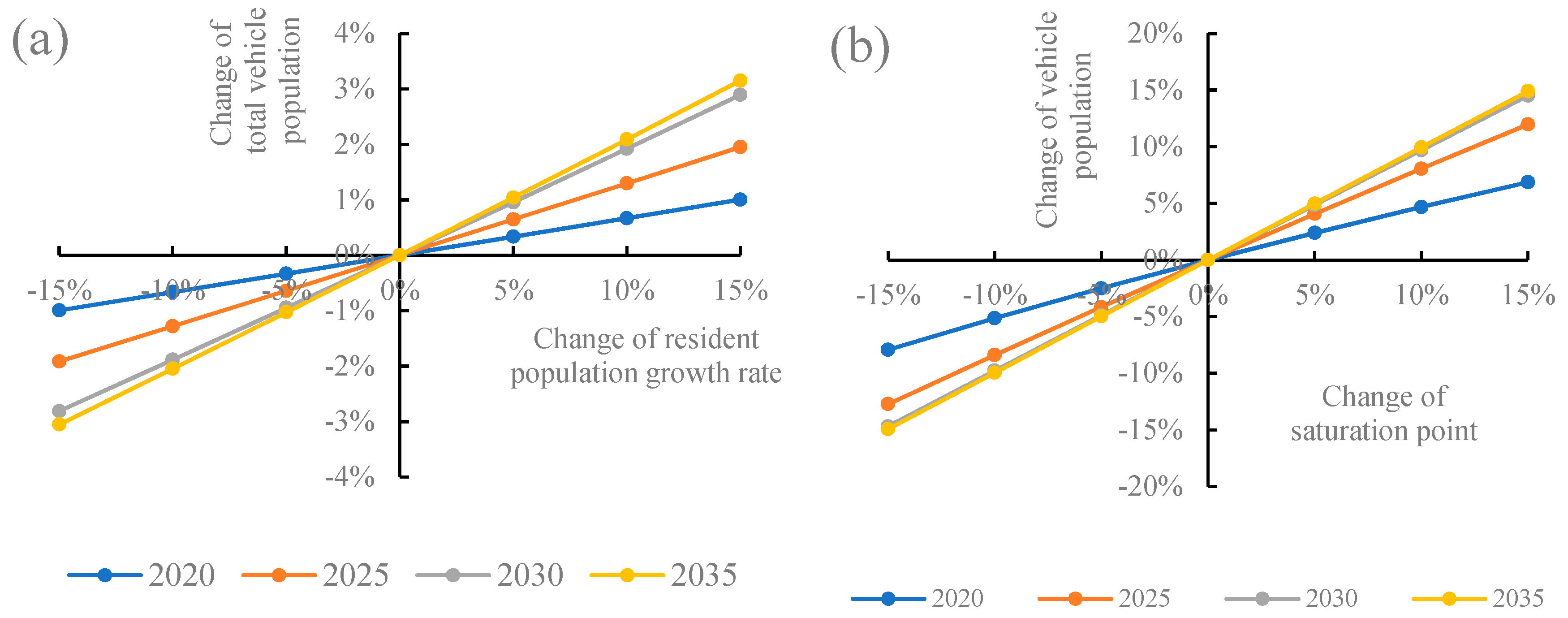
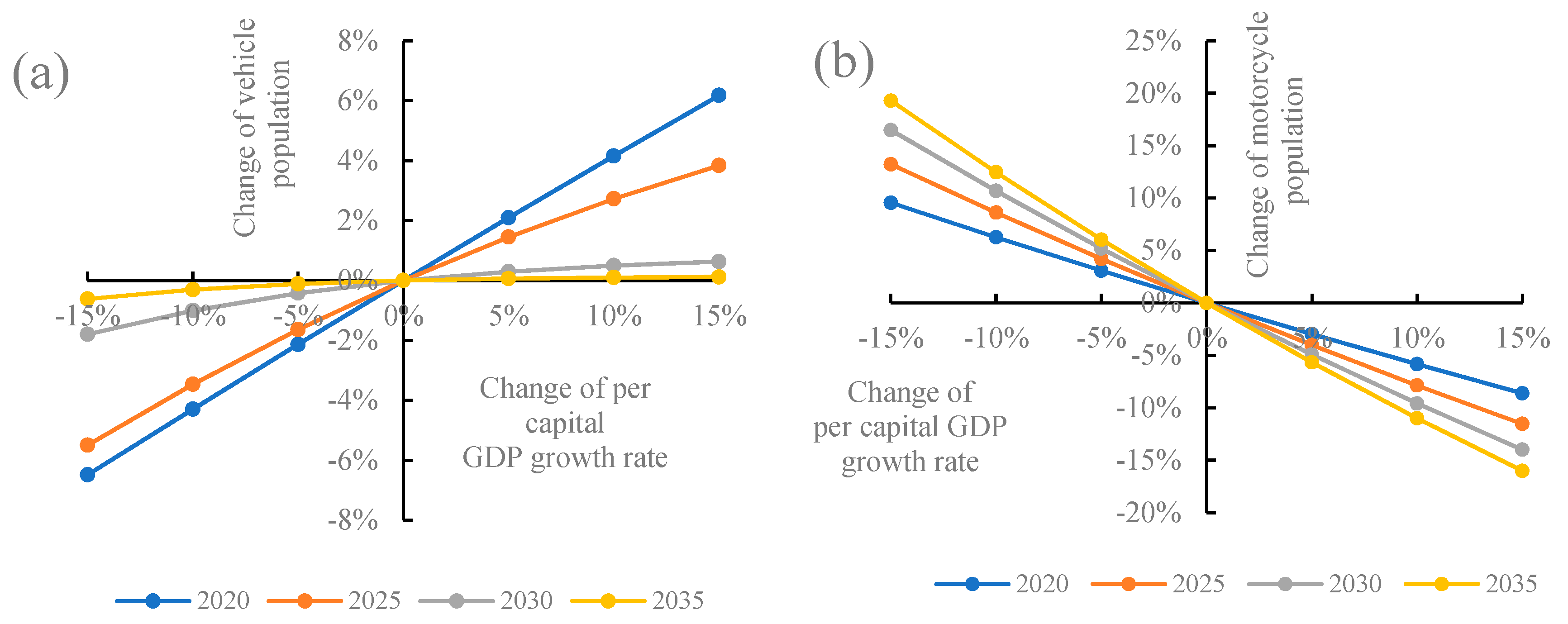
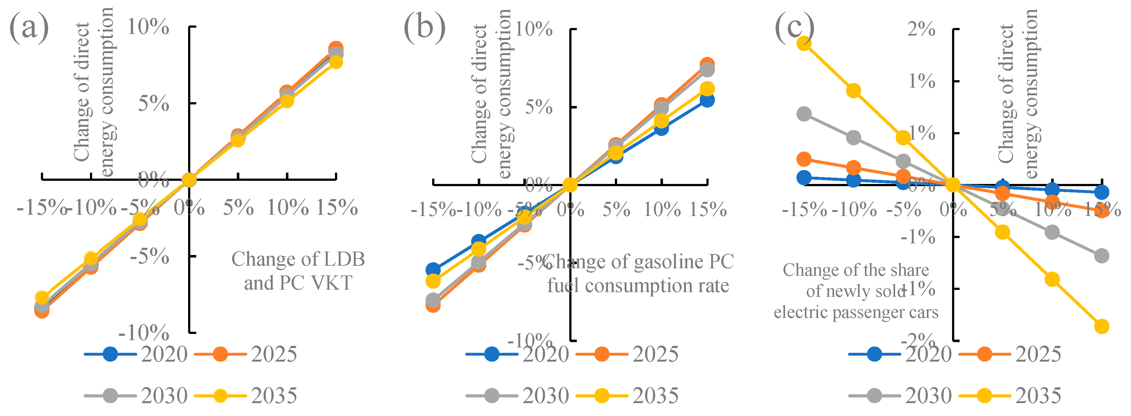
The process involving using models to predict the future vehicle energy consumption and GHG emissions employs the frequent use of postulates and parameter estimations, which have relatively high uncertainties. Despite the use of authoritative references to reduce these uncertainties, it is necessary to analyze uncertainties that exist in this study and that are closely related to the results of the model simulation. In this part, a few key postulates used in this research are selected for a discussion on uncertainties and an assessment of their impact.

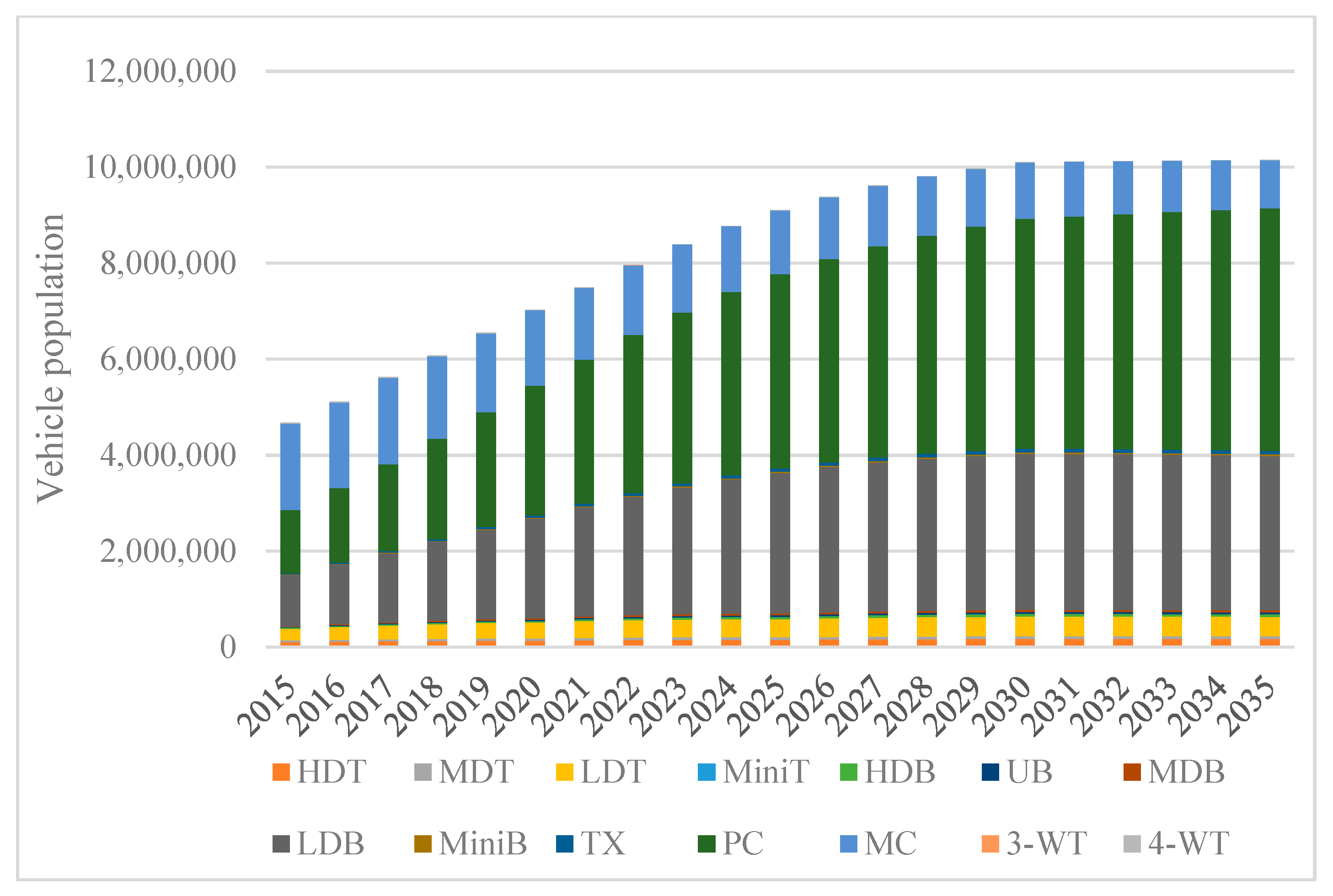
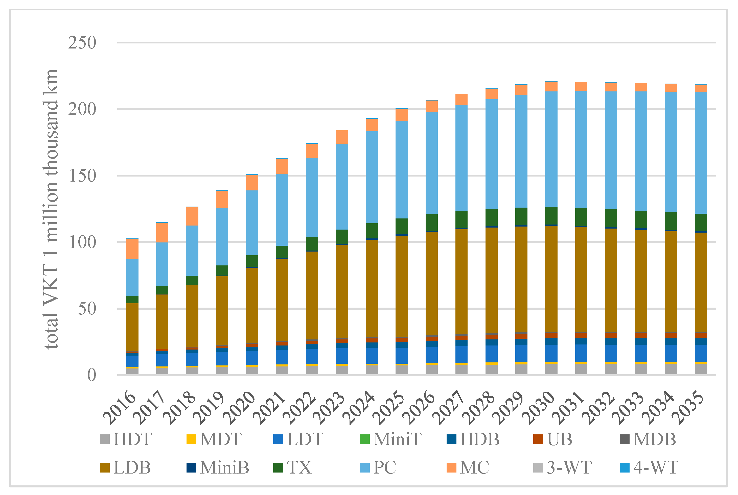
First, this study covers an analysis of the vehicle population, VKT, growth patterns of the population, and the economy in Chongqing City; however, due to difficulties in accessing data at the city level, the fuel-economy statistics at the national level are used for calculations, which might have affected the accuracy of the estimation of the fuel consumption and GHG emissions of vehicles. To improve the accuracy of our calculations, reliable data regarding the fuel economy at the province and city levels need to be provided, which requires not only the efforts of academic institutions, but also cooperation from the respective government agencies.

Second, this study works with a scenario analysis on the future targets of road-transportation low-carbon policies, but, in fact, there will be uncertainty due to human factors during the implementation of the policies. For example, people’s travel needs and behavior changes will affect the choice in terms of their travel mode and people’s willingness to purchase—and the affordability of—new-energy vehicles will affect the actual promotion rate of new-energy vehicles. Therefore, the resolution of these uncertainties requires a more detailed investigation and study in the future.

Based on the research results above, this paper puts forward the following policy suggestions for the low-carbon development of the road-transportation sector in Chongqing and China in the future:

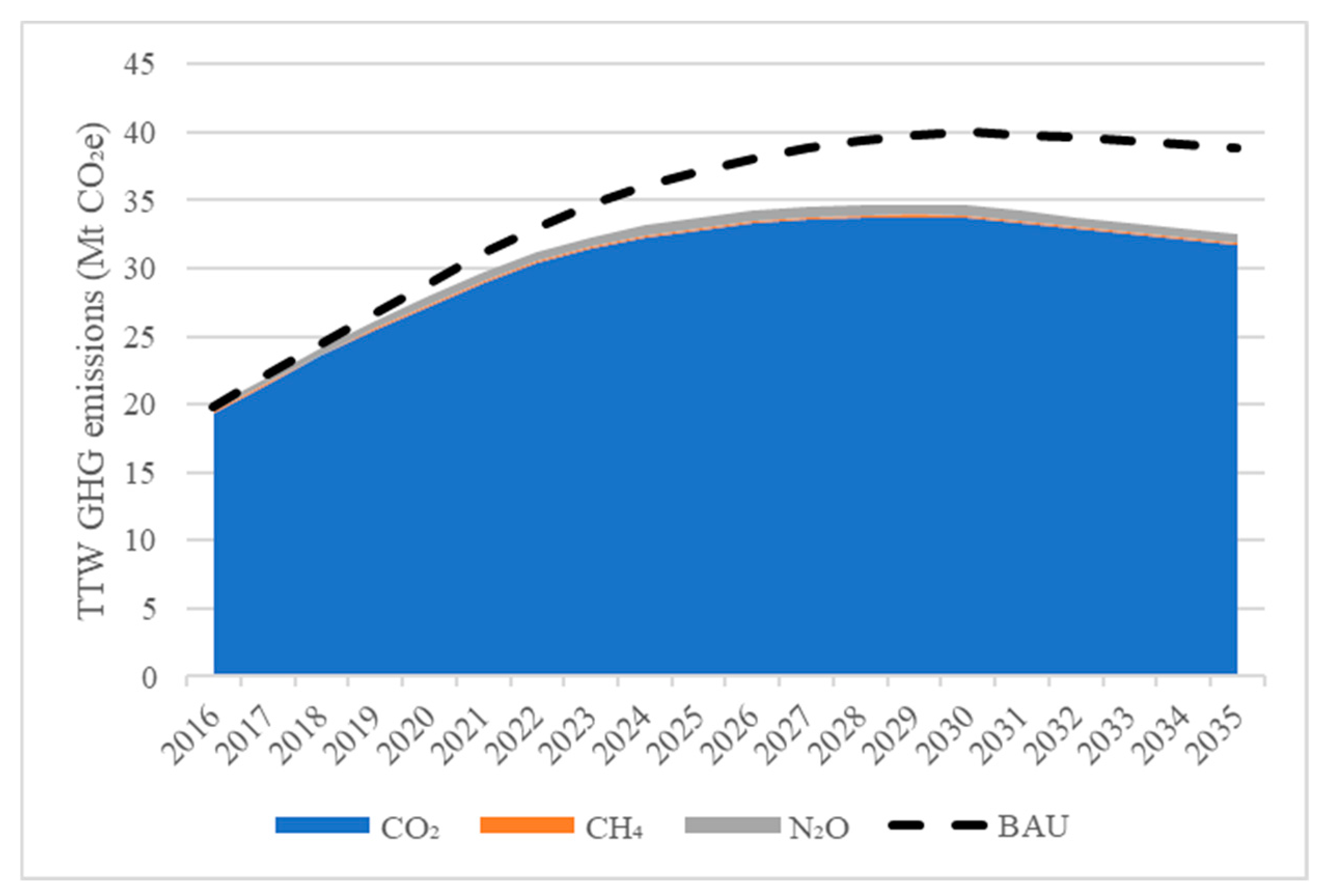
The national government should dominate regions to optimize power-generation energy structures. The GHG emission-reduction effect of new-energy vehicles, especially EVs, is closely related to the electricity-emission factor of the regional power grid. In China, the electricity-emission factor is still high due to the coal-dominated power-generation structure in China when compared to Europe, the USA, and other developed countries. According to the results of our analysis on the TTW and WTW GHG emissions, in the early period of implementing the promotion policy for AFVs, the effect of the WTW GHG emission-reduction policy will not be significant because of the high emission factors of the electricity. With an increase in the ratio of non-fossil energy for power generation, the electricity-emission factor will decrease and the WTW GHG reduction effect, stemming from the policy, will become significant. Therefore, the national and regional governments should continue to optimize the power-generation energy structure, while they promote EVs in the future and should promote the use of non-fossil renewable-energy power generation. As for Chongqing, we suggest that the Chongqing government should take advantage of the regional resources to vigorously develop hydropower, natural-gas power generation, and other clean energies to increase the effect of GHG emission reductions from EVs at the source.

Continue to expand natural-gas vehicle applications. Due to the abundant natural-gas resources in Chongqing, and the surrounding area of the Sichuan Province, the Chongqing government promoted the use of CNG buses and taxis early on and now their share has reached an upper limit of almost 99% at present. There are already many gas filling stations in the main urban area of Chongqing, but the fuel that current PCs use is still mainly gasoline. According to the scenario analysis promoting the AFV policy, the promotion of CNG and LNG vehicles in Chongqing will increase natural-gas energy consumption and, eventually, this will reduce the WTW GHG emissions of the road-transportation sector. In addition, the current Chongqing long-distance HDBs and HDTs still mainly use diesel as fuel. In the future, with adequate resources and sufficient funds, it is recommended that more effort could be made to promote the use of CNG and LNG in the field of PCs and heavy-duty vehicles, and to build gas stations at expressway service points and along key highways.

Develop and implement more effective fuel-economy standards. From the above analysis, we can see that the GHG emission-reduction effect of improving the fuel economy via the conventional-fuel passenger car policy is not very high in the early stage, but, with the cumulative effect of new vehicles, in the medium and long term, the WTW GHG will gradually become significant from 2020 onwards. Therefore, the Chongqing government and the Chinese central government should continue to make and implement fuel-economy standards and encourage the relevant automobile manufacturing enterprises to research and develop new technologies to improve the fuel economy through vehicle lightweight technology, reduced air-resistance technology, and so on. Moreover, a corresponding measurement assessment and reward-and-punishment system should be built so that, after specific timeframes, the fuel economy of any new vehicles from automobile manufacturing enterprises can be tested under actual road conditions.

Last, according to the results of this study, the two policies we analyzed will have a hedging effect on the direct energy consumption and GHG emission reductions, and, with improvements in vehicle fuel technology and the increasing proportion of new-energy vehicles, in the long term, the hedging effect will become more significant. Therefore, in the future, the policy makers in Chongqing or in similar cities across China might like to consider enhancing both policies and introducing or enhancing some other road-transportation policy options, such as reducing the purchase tax on motorcycles to encourage residents to buy and use more motorcycles instead of PCs and reducing bus ticket fees or increasing bus lanes to encourage residents to travel by bus to further reduce the energy consumption and GHG emissions generated by PCs. The specific GHG emission-reduction effects of these policy options can be further investigated and studied in the future.

5. Conclusions

Based on our previous research, this paper takes Chongqing City as an example and, using a bottom-up method to predict the motor-vehicle population by vehicle type and fuel structure, it estimates the energy demand and GHG emissions of road transportation at the city level from 2015 to 2035 under the BAU and other policy scenarios, including single-policy implementation scenarios for improving the fuel economy via the conventional-fuel passenger car policy, promoting AFVs, and a mixed-policy scenario. Moreover, this study analyzes the interaction effects of the policies and compares the evaluation results of the mixed policy with the evaluation results under the individual policy-implementation scenarios. We then discuss the causes of the interaction effect from the mixed policy. The main conclusions from the study are presented below:

(1)

The total population of motor vehicles in Chongqing will increase from 4.61 million in 2015 to 10.10 million in 2030 and reach saturation point at 10.15 million in 2035. The population of passenger cars will exceed motorcycles and will see the largest increase in the future;

(2)

in the BAU scenario, the road-transportation energy demand in Chongqing will keep increasing from 2015 and will peak at 576,437 TJ in 2030, before it begins to decline to 559,411 TJ by 2035. The trends for the TTW and WTW GHG emissions are similar to that of the energy demand. The WTW GHG emissions will increase from 24.9 Mt CO₂e in 2016 to 50.5 Mt CO₂e in 2030 and will then gradually decline to 48.9 Mt CO₂e in 2035;

(3)

in the IFE scenario, with improvements in the fuel economy of conventional passenger cars, the total vehicle direct energy demand will peak in 2029, one year earlier than in the BAU scenario and, compared to the BAU scenario, the WTW GHG emissions will reduce by 4.0%, 14.6%, and 17.4% in 2020, 2030, and 2035, respectively. In the PAFV scenario, more alternative vehicles, including EVs, PHEVs, CNG, and LNG vehicles, will gradually diffuse into the market. The total vehicle direct energy demand will peak in 2027, three years earlier than in the BAU scenario, and the WTW GHG emissions will reduce by 1.3%, 10.3%, and 18.2% in 2020, 2030, and 2035, respectively, peaking in 2028; and

(4)

the two types of policies have a hedging effect on the direct energy-consumption saving, TTW GHG emission reductions, and WTW GHG emission reductions. In the PM scenario, with the mixed policy being inclusive of the two types of policies, the WTW GHG emissions will reduce by 5.1%, 22.0%, and 29.4% in 2020, 2030, and 2035. respectively, and the WTW GHG emission reduction will be lower than the sum of WTW GHG emission-reduction effects from the two single-policy scenarios. The reason for this is that, with an incremental share of AFVs, the share of conventional-fuel vehicles will decrease, which indirectly reduces the fuel-consumption saving caused by the separate implementations for improving the fuel economy via the conventional-fuel passenger car policy, resulting in a hedging effect from these two types of policies.

In view of the above results from our analysis, this study proposes some policy implications to provide a reference for the formulation and adjustment of Chongqing’s—or even China’s—low-carbon road-transportation policies in the future. The work carried out for this study can provide a reference to help policy makers to develop and adjust their low-carbon transportation policies for cities and regions around the world in the future.

References

1. IEA. Key World Energy Statistics 2017. International Energy Agency: Paris, France, 2017. Available online: http://www.iea.org/publications/freepublications/publication/KeyWorld2017.pdf (accessed on 30 May 2018).
2. Fridstrøm, L.; Østli, V. The vehicle purchase tax as a climate policy instrument. Transp. Res. Part A Policy Pract. 2017, 96, 168–189. [Google Scholar] [CrossRef]
3. Wang, S.; Zhao, J. The distributional effects of lotteries and auctions—License plate regulations in Guangzhou. Transp. Res. Part A Policy Pract. 2017, 106, 473–483. [Google Scholar] [CrossRef]
4. Yang, J.; Liu, Y.; Qin, P.; Liu, A.A. A review of Beijing’s vehicle registration lottery: Short-term effects on vehicle growth and fuel consumption. Energy Policy 2014, 75, 157–166. [Google Scholar] [CrossRef]
5. Simmons, R.A.; Shaver, G.M.; Tyner, W.E.; Garimella, S.V. A benefit-cost assessment of new vehicle technologies and fuel economy in the U.S. market. Appl. Energy 2015, 157, 940–952. [Google Scholar] [CrossRef]
6. Zhang, X.; Bai, X. Incentive policies from 2006 to 2016 and new energy vehicle adoption in 2010–2020 in China. Renew. Sustain. Energy Rev. 2017, 70, 24–43. [Google Scholar] [CrossRef]
7. Wang, H.; Zhang, X.; Ouyang, M. Energy consumption of electric vehicles based on real-world driving patterns: A case study of Beijing. Appl. Energy 2015, 157, 710–719. [Google Scholar] [CrossRef]
8. Onat, N.C.; Kucukvar, M.; Tatari, O. Conventional, hybrid, plug-in hybrid or electric vehicles? State-based comparative carbon and energy footprint analysis in the United States. Appl. Energy 2015, 150, 36–49. [Google Scholar] [CrossRef]
9. Peterson, M.B.; Barter, G.E.; West, T.H.; Manley, D.K. A parametric study of light-duty natural gas vehicle competitiveness in the United States through 2050. Appl. Energy 2014, 125, 206–217. [Google Scholar] [CrossRef]
10. Gambhir, A.; Tse, L.K.C.; Tong, D.; Martinez-Botas, R. Reducing China’s road transport sector CO2 emissions to 2050: Technologies, costs and decomposition analysis. Appl. Energy 2015, 157, 905–917. [Google Scholar] [CrossRef]
11. Cheng, Y.-H.; Chang, Y.-H.; Lu, I.J. Urban transportation energy and carbon dioxide emission reduction strategies. Appl. Energy 2015, 157, 953–973. [Google Scholar] [CrossRef]
12. Huo, H.; Zheng, B.; Wang, M.; Zhang, Q.; He, K. Bin Vehicular air pollutant emissions in China: Evaluation of past control policies and future perspectives. Mitig. Adapt. Strateg. Glob. Chang. 2015, 20, 719–733. [Google Scholar] [CrossRef]
13. Malayath, M.; Verma, A. Activity based travel demand models as a tool for evaluating sustainable transportation policies. Res. Transp. Econ. 2013, 38, 45–66. [Google Scholar] [CrossRef]
14. Hoogwijk, M.; de la Rue du Can, S.; Novikova, A.; Urge-Vorsatz, D.; Blomen, E.; Blok, K. Assessment of bottom-up sectoral and regional mitigation potentials. Energy Policy 2010, 38, 3044–3057. [Google Scholar] [CrossRef]
15. Lutsey, N.; Sperling, D. Greenhouse gas mitigation supply curve for the United States for transport versus other sectors. Transp. Res. Part D Transp. Environ. 2009, 14, 222–229. [Google Scholar] [CrossRef]
16. Tessum, C.W.; Hill, J.D.; Marshall, J.D. Life cycle air quality impacts of conventional and alternative light-duty transportation in the United States. Proc. Natl. Acad. Sci. USA 2014, 111, 18490–18495. [Google Scholar] [CrossRef] [PubMed] [Green Version]
17. Wang, C.; Cai, W.; Lu, X.; Chen, J. CO2 mitigation scenarios in China’s road transport sector. Energy Convers. Manag. 2007, 48, 2110–2118. [Google Scholar] [CrossRef]
18. He, K.; Huo, H.; Zhang, Q.; He, D.; An, F.; Wang, M.; Walsh, M.P. Oil consumption and CO2 emissions in China’s road transport: Current status, future trends, and policy implications. Energy Policy 2005, 33, 1499–1507. [Google Scholar] [CrossRef]
19. Yan, X.; Crookes, R.J. Reduction potentials of energy demand and GHG emissions in China’s road transport sector. Energy Policy 2009, 37, 658–668. [Google Scholar] [CrossRef]
20. Huo, H.; Wang, M.; Zhang, X.; He, K.; Gong, H.; Jiang, K.; Jin, Y.; Shi, Y.; Yu, X. Projection of energy use and greenhouse gas emissions by motor vehicles in China: Policy options and impacts. Energy Policy 2012, 43, 37–48. [Google Scholar] [CrossRef]
21. Ou, X.; Zhang, X.; Chang, S. Scenario analysis on alternative fuel/vehicle for China’s future road transport: Life-cycle energy demand and GHG emissions. Energy Policy 2010, 38, 3943–3956. [Google Scholar] [CrossRef]
22. Hartgen, D.T.; Fields, M.G.; Scott, M.; Jose, E.S.; San Jose, E.; Moore, A.T. Impacts of Transportation Policies on Greenhouse Gas Emissions in U.S. Regions; Reason Foundation: Los Angeles, CA, USA, 2011. [Google Scholar]
23. Moore, A.T.; Staley, S.R.; Poole, R.W. The role of VMT reduction in meeting climate change policy goals. Transp. Res. Part A Policy Pract. 2010, 44, 565–574. [Google Scholar] [CrossRef]
24. Silva-Send, N.; Anders, S.; Narwold, A. Cost effectiveness comparison of certain transportation measures to mitigate greenhouse gas emissions in San Diego county, California. Energy Policy 2013, 62, 1428–1433. [Google Scholar] [CrossRef]
25. Zheng, B.; Zhang, Q.; Borken-Kleefeld, J.; Huo, H.; Guan, D.; Klimont, Z.; Peters, G.P.; He, K. How will greenhouse gas emissions from motor vehicles be constrained in China around 2030? Appl. Energy 2015, 156, 230–240. [Google Scholar] [CrossRef] [Green Version]
26. Peng, T.; Ou, X.; Yuan, Z.; Yan, X.; Zhang, X. Development and application of China provincial road transport energy demand and GHG emissions analysis model. Appl. Energy 2018, 222, 313–328. [Google Scholar] [CrossRef]
27. He, D.; Liu, H.; He, K.; Meng, F.; Jiang, Y.; Wang, M.; Zhou, J.; Calthorpe, P.; Guo, J.; Yao, Z.; Wang, Q. Energy use of, and CO2 emissions from China’s urban passenger transportation sector—Carbon mitigation scenarios upon the transportation mode choices. Transp. Res. Part A Policy Pract. 2013, 53, 53–67. [Google Scholar] [CrossRef]
28. Orsi, F.; Muratori, M.; Rocco, M.; Colombo, E.; Rizzoni, G. A multi-dimensional well-to-wheels analysis of passenger vehicles in different regions: Primary energy consumption, CO2 emissions, and economic cost. Appl. Energy 2016, 169, 197–209. [Google Scholar] [CrossRef]
29. Wu, Y.; Yang, Z.; Lin, B.; Liu, H.; Wang, R.; Zhou, B.; Hao, J. Energy consumption and CO2 emission impacts of vehicle electrification in three developed regions of China. Energy Policy 2012, 48, 537–550. [Google Scholar] [CrossRef]
30. Zhou, G.; Ou, X.; Zhang, X. Development of electric vehicles use in China: A study from the perspective of life-cycle energy consumption and greenhouse gas emissions. Energy Policy 2013, 59, 875–884. [Google Scholar] [CrossRef]
31. Zeng, Y.; Tan, X.; Gu, B.; Wang, Y.; Xu, B. Greenhouse gas emissions of motor vehicles in Chinese cities and the implication for China’s mitigation targets. Appl. Energy 2016, 184, 1016–1025. [Google Scholar] [CrossRef]
32. Zhang, G.; Zhu, J. Analysis and prediction of China’s motorcycle market. Forecasting 1996, 5, 37–41. (In Chinese) [Google Scholar]
33. Hao, H.; Wang, H.W.; Ouyang, M.G.; Cheng, F. Vehicle survival patterns in China. Sci. China Technol. Sci. 2011, 54, 625–629. [Google Scholar] [CrossRef]
34. Department of Social Development of the National Development and Reform Commission. Full Implementation of a Couple’s Policy of Having Two Children. Available online: http://shs.ndrc.gov.cn/shfzdt/201511/t20151110_758020.html (accessed on 30 May 2018).
35. Deng, Y.; Liu, S.; Cai, J.; Lu, X. Analysis method and demonstration of the evolution of inter provincial population spatial pattern in China. J. Geogr. 2014, 69, 1473–1486. (In Chinese) [Google Scholar]
36. Yang, Q.; Chen, G.; Ma, N.; Qiao, Q. Study on the motor vehicle share ratio in the downtown of Chongqing. J. Southwest China Norm. Univ. 2009, 34, 173–177. (In Chinese) [Google Scholar]
37. Wang, T. The Research of the Vehicular Emission Inventory in the Urban of Chongqing Based on IVE Model. Master’s Thesis, Chongqing Jiaotong University, Chongqing, China, 31 December 2013. (In Chinese). [Google Scholar]
38. Gao, Y.; Yu, M.; Yu, Y. Study on the quantitative model of urban public transport typical energy saving technology comprehensive transportation. China Transp. Rev. 2013, 5, 27–31. (In Chinese) [Google Scholar]
39. Chung, W.; Zhou, G.; Yeung, I.M.H. A study of energy efficiency of transport sector in China from 2003 to 2009. Appl. Energy 2013, 112, 1066–1077. [Google Scholar] [CrossRef]
40. Huo, H.; Wang, M.; Johnson, L.; He, D. Projection of Chinese Motor Vehicle Growth, Oil Demand, and CO2 Emissions through 2050. Transp. Res. Rec. J. Transp. Res. Board 2007, 2038, 69–77. [Google Scholar] [CrossRef]
41. Huo, H.; He, K.; Wang, M.; Yao, Z. Vehicle technologies, fuel-economy policies, and fuel-consumption rates of Chinese vehicles. Energy Policy 2012, 43, 30–36. [Google Scholar] [CrossRef]
42. Davis, S.C.; Williams, S.E.; Boundy, R.G. Transportation energy data book: Edition 29. Energy Conserv. Consum. Utilization 2015, 176, 319–338. [Google Scholar]
43. US Census Bureau. Vehicle Inventory and Use Survey. 1977–2002. Available online: https://www.census.gov/svsd/www/vius/products.html (accessed on 30 May 2018).
44. Technology Roadmap for Energy Saving and New Energy Vehicles Strategic Advisory Committee, Society of Automotive Engineers of China. Technology Roadmap for Energy Saving and New Energy Vehicles, 1st ed.; China Machine Press: Beijing, China, 2017; pp. 131–132. ISBN 978-7-111-55081-5. (In Chinese) [Google Scholar]
45. Rahman, M.M.; Canter, C.; Kumar, A. Well-to-wheel life cycle assessment of transportation fuels derived from different North American conventional crudes. Appl. Energy 2015, 156, 159–173. [Google Scholar] [CrossRef]
46. Liu, Z.; Guan, D.; Wei, W.; Davis, S.J.; Ciais, P.; Bai, J.; Peng, S.; Zhang, Q.; Hubacek, K.; Marland, G.; et al. Reduced carbon emission estimates from fossil fuel combustion and cement production in China. Nature 2015, 524, 335–338. [Google Scholar] [CrossRef] [PubMed] [Green Version]
47. Myhre, G.; Shindell, D.; Bréon, F.-M.; Collins, W.; Fuglestvedt, J.; Huang, J.; Koch, D.; Lamarque, J.-F.; Lee, D.; Mendoza, B.; et al. Anthropogenic and natural radiative forcing. In Climate Change 2013: The Physical Science Basis. Contribution of Working Group I to the Fifth Assessment Report of the Intergovernmental Panel on Climate Change; Cambridge University Press: Cambridge, UK; New York, NY, USA, 2013. [Google Scholar]
48. China Energy Research Association. China Energy Outlook 2030, 1st ed.; Economic & Management Publishing House: Beijing, China, 2016; pp. 193–215. ISBN 978-7-5096-4329-7. (In Chinese) [Google Scholar]
Figure 1. Causal chain of improving the fuel-economy policy.
Sustainability 10 02033 g001
Figure 2. Causal chain of promoting the development of the AFVs policy.
Sustainability 10 02033 g002
Figure 3. Vehicle population of vehicle types in Chongqing 2015–2035.
Sustainability 10 02033 g003
Figure 4. Vehicle kilometers travelled of vehicle types in Chongqing 2016–2035.
Sustainability 10 02033 g004
Figure 5. Direct energy demand of the road transport sector in Chongqing under IFE scenario.
Sustainability 10 02033 g005
Figure 6. Direct energy demand of the road transport sector in Chongqing under PAFV scenario.
Sustainability 10 02033 g006
Figure 7. Direct energy demand of the road transport sector in Chongqing under PM scenario.
Sustainability 10 02033 g007
Figure 8. 2016–2035 Direct energy savings of the road transport sector in Chongqing.
Sustainability 10 02033 g008
Figure 9. 2016–2035 WTW GHG emissions of the road transport sector in Chongqing.
Sustainability 10 02033 g009
Figure 10. 2016–2035 Please define this term. GHG emissions of the road transport sector in Chongqing.
Sustainability 10 02033 g010
Figure 11. Sensitivity analysis on (a) the effect of resident population growth rate on the total motor vehicle population projection and (b) the vehicle saturation point on the motor vehicle population projection (except for motorcycles).
Sustainability 10 02033 g011
Figure 12. Sensitivity analysis on (a) the effect of per capita GDP growth rate on the motor vehicle population projection (except for motorcycles) and (b) on the motorcycle population projection.
Sustainability 10 02033 g012
Figure 13. Sensitivity analysis on the (a) effect of VKT change of LDBs and PCs, (b) effect of gasoline PC fuel consumption rate, and (c) effect of the fuel share of newly sold electric passenger cars on the direct energy consumption.
Sustainability 10 02033 g013