Article

Relationship between Rural Built Environment and Household Vehicle Ownership: An Empirical Analysis in Rural Sichuan, China

1
Business School, Sichuan University, Chengdu 610065, Sichuan, China
2
College of Environment and Civil Engineering, Chengdu University of Technology, Chengdu 610059, Sichuan, China
3
Department of the Built Environment, Eindhoven University of Technology, 5600 MB Eindhoven, The Netherlands
4
Department of Engineering Management, Sichuan College of Architectural Technology, Deyang 618000, Sichuan, China
*
Authors to whom correspondence should be addressed.
Sustainability 2018, 10(5), 1566; https://doi.org/10.3390/su10051566
Submission received: 26 April 2018 / Revised: 5 May 2018 / Accepted: 10 May 2018 / Published: 14 May 2018
(This article belongs to the Section Sustainable Transportation)

Abstract

:
With the rapid rural urbanization and new rural construction in China, tremendous changes are occurring in rural built environments and rural household vehicle ownership. However, few studies have examined the relationship between rural built environments and rural household vehicle ownership. In this study, a questionnaire survey of 374 rural households was conducted and the built environment data of seven typical villages in rural Sichuan were collected using Geographic Information System (GIS) technology and on-site measurement. This study aimed to investigate the relationship between the rural built environment and rural household vehicle ownership in China through a multinomial logit (MNL) model. Results show that household structure attributes have the most significant relationship with vehicle ownership, followed by rural built environment attributes and the respondents’ driving skills. In the process of urbanization, with increases in building density, road density, and destination accessibility, an increase in high-carbon vehicle ownership is an inevitable trend among rural households. However, low-carbon-oriented rural planning can effectively control the increase in high-carbon vehicle ownership. For example, the distance between rural households and important destinations, such as hospitals, schools, and markets, should be shortened and rural residents should be encouraged to learn to ride bicycles. Moreover, rural residents riding motorcycles can effectively reduce household car ownership.

1. Introduction

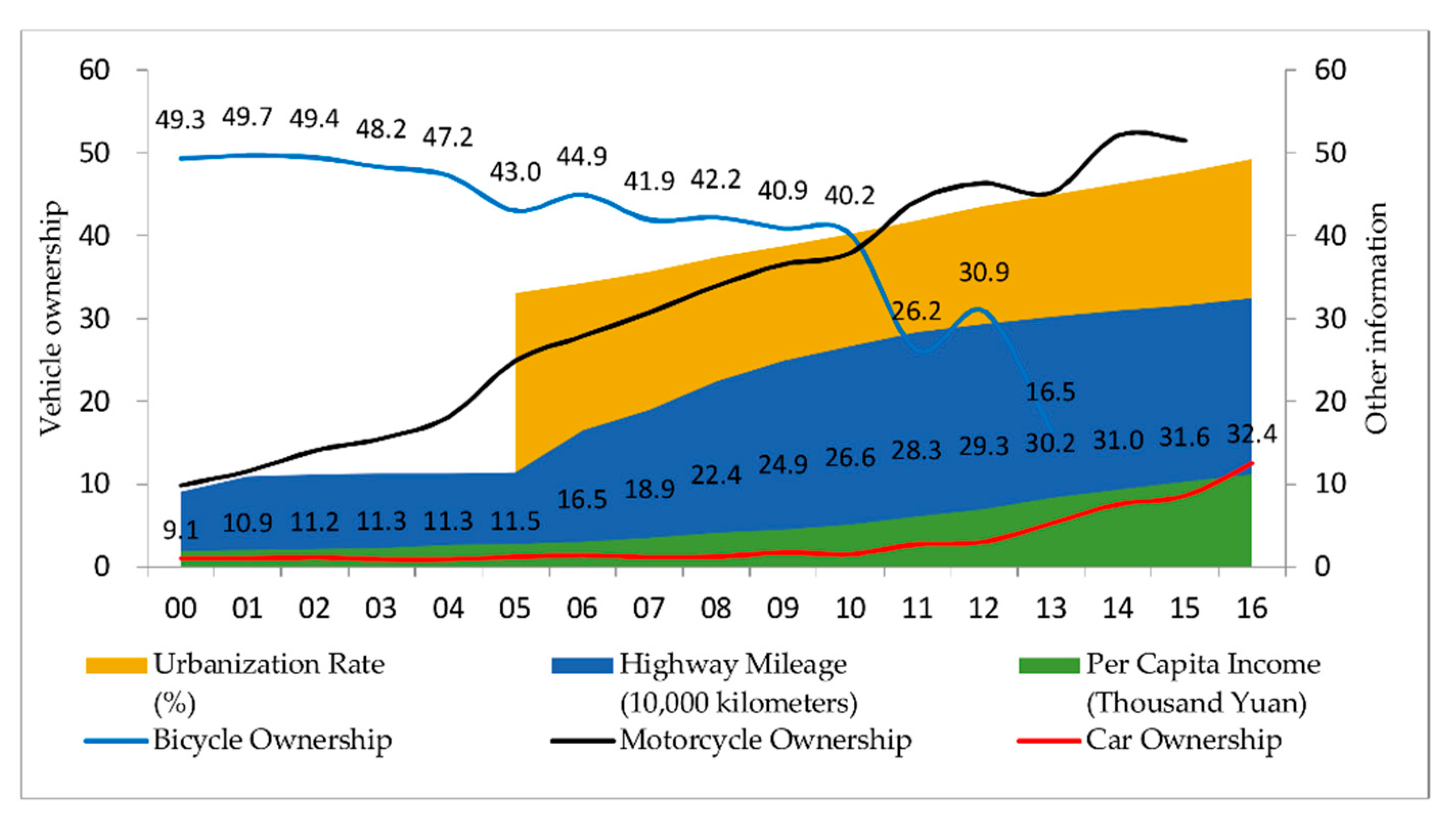
In 1978, China launched internal reforms that began with rural areas. After 40 years, rural China has undergone tremendous changes. By the end of 2016, the fixed-asset investment of rural households was 20.83 times that in 1985 and 3.43 times that in 2000; the disposable income of rural residents was 31.10 times that in 1985 and 5.49 times that in 2000 [1]. The gap between urban and rural areas is gradually narrowing with the rapid urbanization. By the end of 2016, China’s highway mileage reached 4,696,263 km, which was 3.35 times that in 2000 [1]. In the process of rural urbanization and new rural construction, temporal and spatial changes have occurred in built environments, and these changes have directly influenced household vehicle ownership. For example, in 2012, the number of bicycles per 100 households in rural China (79.00) was 0.66 times that in 2000 (120.50); in 2016, the number of motorcycles per 100 households in rural China (65.10) was 2.97 times that in 2000 (21.90); in 2016, the number of cars per 100 households in rural China (17.4) was 13.18 times that in 2000 (1.32) [1]. In Western developed countries, the rapid increase of high-carbon vehicle ownership and the reliance on cars have caused many problems. For example, the annual growth rate of fossil fuel demand in the transportation sector has reached 10.56% [2]. Moreover, automobiles have become the main cause of air pollution and photochemical smog pollution in China [3,4]. In addition, traffic congestion and obesity are also caused by people’s dependence on automobiles [3,5,6]. China is the most populous country in the world, thus a small increase in automobile ownership per capita will result in huge increases in energy consumption and carbon dioxide emissions. By the end of 2016, China’s rural population accounted for 42.65% of the total population of the country, along with tremendous changes in rural built environments. Thus, studying the relationship between rural built environments and rural household vehicle ownership is of great significance for energy conservation and traffic emission reduction. Household vehicle ownership and related information in rural China is shown in Figure 1. The x-axis reports the years from 2000 to 2016, abbreviated with the last two digits. The left y-axis reports the number of vehicles per 100 rural households, while the right y-axis reports urbanization rate (%), highway mileage (100,000 km), and per capita income of rural residents (1000 yuan). Obviously, in Figure 1 all the indicators show an increasing trend, except for bicycle ownership.
The present study divides rural household vehicles into low-carbon (bicycles and electric bicycles) and high-carbon (motorcycles and automobiles) vehicles. We use a multinomial logit (MNL) model to investigate the effects of the built environment on household vehicle ownership after controlling for household structure attributes and individual driving skills in rural Sichuan, China.
The structure of this paper is as follows. Section 2 reviews previous studies on the relationship between the built environment and vehicle ownership. Section 3 provides the data collected and the results of the descriptive analyses. Detailed explanations of the variables and the MNL model used in this study are presented in Section 4. The results and discussion of the MNL model are presented in Section 5. Finally, Section 6 presents the conclusion and policy implications.

2. Literature Review

The “6Ds” of built environment—density, diversity, design, destination accessibility, distance to transit, and demand management—have been widely used [7,8,9,10,11]. Specific measurement indicators for built environment variables are continuously accumulated and enriched [12,13]. The most commonly used measure indicators are shown in Table 1.
In addition to the 6Ds, other indicators are used to measure the built environment, such as traffic or personal safety [14], neighborhood type [15,16], infrastructure characteristics [17], and leisure facilities [18].
A large number of studies have shown that the built environment directly influences vehicle ownership. However, most empirical studies have focused on the relationship between the built environment and car ownership. Household car ownership decreases within creased built environment density [6,19,20,21,22,23]. Diversity is negatively correlated with car ownership [6,8,22,23,24,25,26]. Ewing et al. [21] and Hong et al. [25] found that road network density is also negatively correlated with household car ownership; however, the effect of design on car ownership is weaker than the effects of density and diversity [26]. Destination accessibility is a built environment index at the regional level and generally includes distance to central business district (CBD) and job accessibility [27,28]. Empirical studies have shown that vehicle ownership decreases with distance to CBD [20,29]. Similarly, distance to CBD can reduce driving mileage significantly and, to a certain degree, the number of family vehicles if the residence is close to the job or business center [6,9]. On the contrary, the demand for and dependence on cars increases with distance from the residence to the CBD [30]. Distance to transit also influences the level of household car ownership. For example, Pltoglou et al. [6] found that the number of cars can be reduced if public transportation stations are within walking distance and that excellent public transportation services will also reduce the number of cars [22]. Demand management usually refers to residential parking distance, number of parking lots, or parking service level. Demand management will increase car ownership if the community has low-cost parking lots [31,32]. Thus, Chatman et al. [33] suggested reducing the number of car parks to impede the increase in car ownership.
Some empirical studies have focused on bicycle, electric bicycle, and motorcycle ownership. Specifically, establishing commercial facilities within 300 ft of the settlement will increase the proportions of public transport use, walking, and cycling, and make using bicycles more feasible [34]. Accessibility, number of bicycle lanes, mixed environment, and street connectivity are positively related to bicycle use, whereas the service level of public transport is negatively related to bicycle use [17].
With regard to motorcycle ownership, Lee and Shiaw [35] (1995) developed a constrained diffusion model of motorcycle ownership and established a model with data obtained in Taiwan. Adults who favorably perceive access to public transport and destinations, presence of sidewalks, and safety from crimes at night are less likely to use motorcycles [36]. Oyedepo et al. [37] found that the likelihood of owning a motorcycle increases 1.43 times with a unit increase in the number of household members; by contrast, the likelihood of owning a motorcycle decreases by 1.66 times and 2.17 times with unit increases in average monthly income and academic qualification of the household head, respectively.
The effects of socio demographic characteristics on household vehicle ownership are stronger than those of the built environment [3]. The main socio demographic characteristics include household size, income, age, education level, occupation, and gender [23,26,38,39].
In the past 16 years, and especially after 2010, the number of household private vehicles has remarkably changed due to the rapid urbanization in China (Figure 1). In comparison with Western developed countries, China possesses certain unique factors that affect vehicle ownership, especially in housing properties such as traditional danwei compounds [2], reformed danwei communities [2], and commodity housing communities [2,3,40]. In the process of urbanization, China’s household hukou is also changing. Although the hukou system is a policy for the distribution of social wealth in the era of planned economy [41], the influence of hukou on Chinese households remains significant. Traffic policy also affects car ownership. One of the most significant characteristics in the literature on the relationship between the built environment and car ownership in China is that the study areas are mainly concentrated in large cities, such as Beijing, Guangzhou, Nanjing, and Jinan [3,42,43,44]. The current study is one of the first to relate the rural built environment to household vehicle ownership in the rural context [45]. This study can provide policy-makers and rural planners with insights into ecological rural construction and low-carbon travel behavior.

3. Data and Variables

3.1. Rural Context in Sichuan

The total economic output of Sichuan Province ranks sixth in China and first in the western part of the country, and its per capita gross domestic product (GDP) exceeds $4000. With rural urbanization and new rural construction, the built environment and household vehicle ownership have changed dramatically. By the end of 2016, the total rural population in Sichuan Province was 41.96 million, and the urbanization rate was 49.12%; the total highway mileage was 324,200 km, which was 3.57 times the mileage in 2000; per capital income was 11,203 yuan, which was 5.89 times that in 2000; and the number of cars per 100 households in rural areas was 12.5, which was 12.38 times that in 2010. By the end of 2015, the number of motorcycles per 100 households was 51.5, which was 5.23 times that in 2000. By the end of 2013, the number of bicycles per 100 households was 16.45, which was 0.33 times that in 2000. Household vehicle ownership and related information on rural Sichuan from 2000 to 2016 are shown in Figure 2. The x-axis reports the years from 2000 to 2016 and are abbreviated with the last two digits. The left y-axis reports the number of vehicles per 100 rural households, while the right y-axis reports China’s urbanization rate (%), highway mileage (10,000 km), and per capita income for rural residents (1000 yuan). Obviously, in Figure 2 all the indicators show an increasing trend except for bicycle ownership in rural Sichuan.

3.2. Sampling and Rural Household Survey

The College of Environment and Civil Engineering of Chengdu University of Technology and the Business School of Sichuan University organized a rural household survey and collected GIS data from 1 October 2017, to 31 January 2018, based on research experiences in 2016 and 2017. The survey sample villages had to meet two conditions: (1) each village had to have at least one local undergraduate or graduate student, and the residents had to be willing to participate in the questionnaire survey; and (2) at least one road was directly accessible to the village, and the roads were all hardened. The latter condition is a basic prerequisite for rural residents to have cars. From 117 sample villages with local students, seven sample villages were identified, including three concentrated-living new villages (Yan Jing, Dong Xing, and Shang Teng) and fours cattered-living traditional villages (Da Zhuang, Shuang Yan, Xin Long, and Wu Gang).
The initial survey questions were developed from previous studies, and the questionnaire was sent to the 117 rural students who were asked to complete the survey. Thereafter, a meeting was organized with the 117 students to discuss the survey questions one by one. On the basis of the discussion, the questionnaire was revised and improved in accordance with the actual situation of rural Sichuan.
From the 117 students, 30 surveyors, comprising 13 graduate and 17 undergraduate students, were completely recruited. All surveyors were uniformly trained before conducting the survey. It is hard to organize a household survey in a rural area, and this was a long questionnaire. We had to make full preparation to guarantee smooth progress of the survey. Thus, preinvestigation was needed to understand the residents’ responses to the survey, how long it would take to complete the questionnaire, and what kind of gift could attract residents to participate. In order to understand the problems that could arise, we randomly selected two sample villages from the seven and randomly investigated five households to complete the questionnaire in each selected village. Finally, we completed 10 preinvestigated questionnaires and found some problems: (1) rural residents lacked patience to complete the questionnaire; (2) incentives had a significant effect on encouraging residents to complete the questionnaire; and (3) residents from different sample villages had different preferences for incentives. Finally, we prepared different incentives (mainly household goods and food) according to the preferences of the respondents who would complete the questionnaire. In the formal investigation, each survey group was led by a local student, and each questionnaire was completed by a face-to-face question-and-answer method between the surveyor and the respondent. Each session lasted 60–80 min.
Two types of questionnaires were used, village and household survey questionnaires. The village survey questionnaire was conducted by the surveyor through an on-site measurement and an interview with the village chief. Rural households were randomly selected by the surveyor to complete the household questionnaire. If the selected household refused to accept the questionnaire, then it would be randomly transferred to the next household.
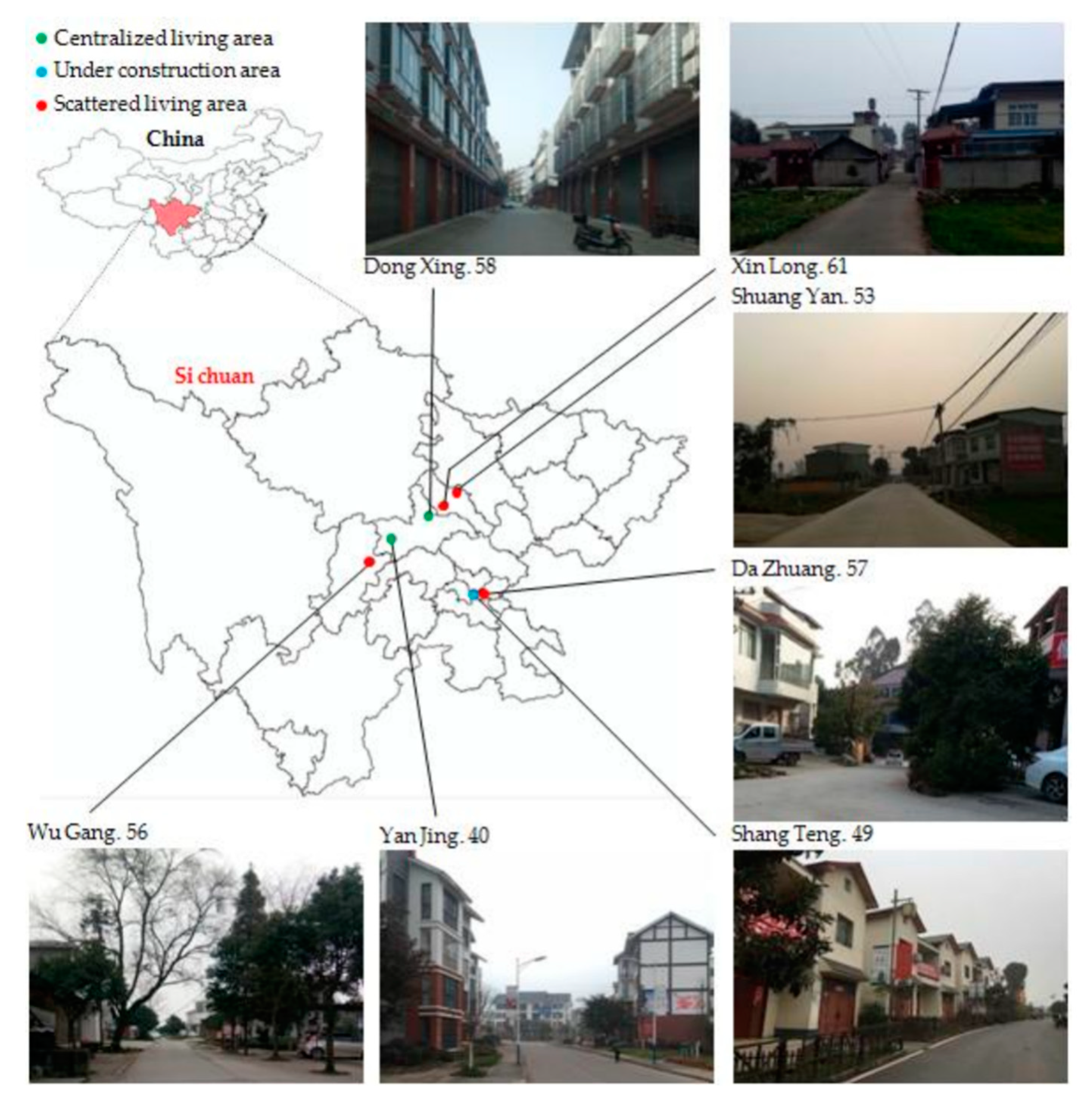
Finally, 413 completed questionnaires were returned, and 34 were eliminated because of missing data. The effective questionnaire rate was 90.56%. Thus, we obtained 374 valid household and seven valid village questionnaires involving 1758 and 16,953 respondents, respectively. The actual built environment, the regional location, and the number of valid questionnaires of the seven sample villages are shown in Figure 3.
The household structure attributes and vehicle ownership of the households in the sample villages were in good agreement with the statistical data of China and Sichuan in the China Statistical Yearbook. However, the questionnaire survey value of rural household car ownership was significantly higher than the value in the China Statistical Yearbook. This significant difference was mainly attributed to three reasons: (1) The household cars in this survey included all four-wheeled motor vehicles owned by rural households, including small cars, passenger cars, and small transport vehicles. (2) In China’s rural areas, some residents go out to work and do not always live in the village, therefore some households’ cars are not always in the village. The number of household cars used in this paper includes the cars that are not always in the village. (3) The level of infrastructure construction and economic development in the sample villages was higher than the average in China and Sichuan. The households in the sample villages were randomly selected, thus they were adequately representative of the villages. A comparison of the sample and population characteristics is shown in Table 2.
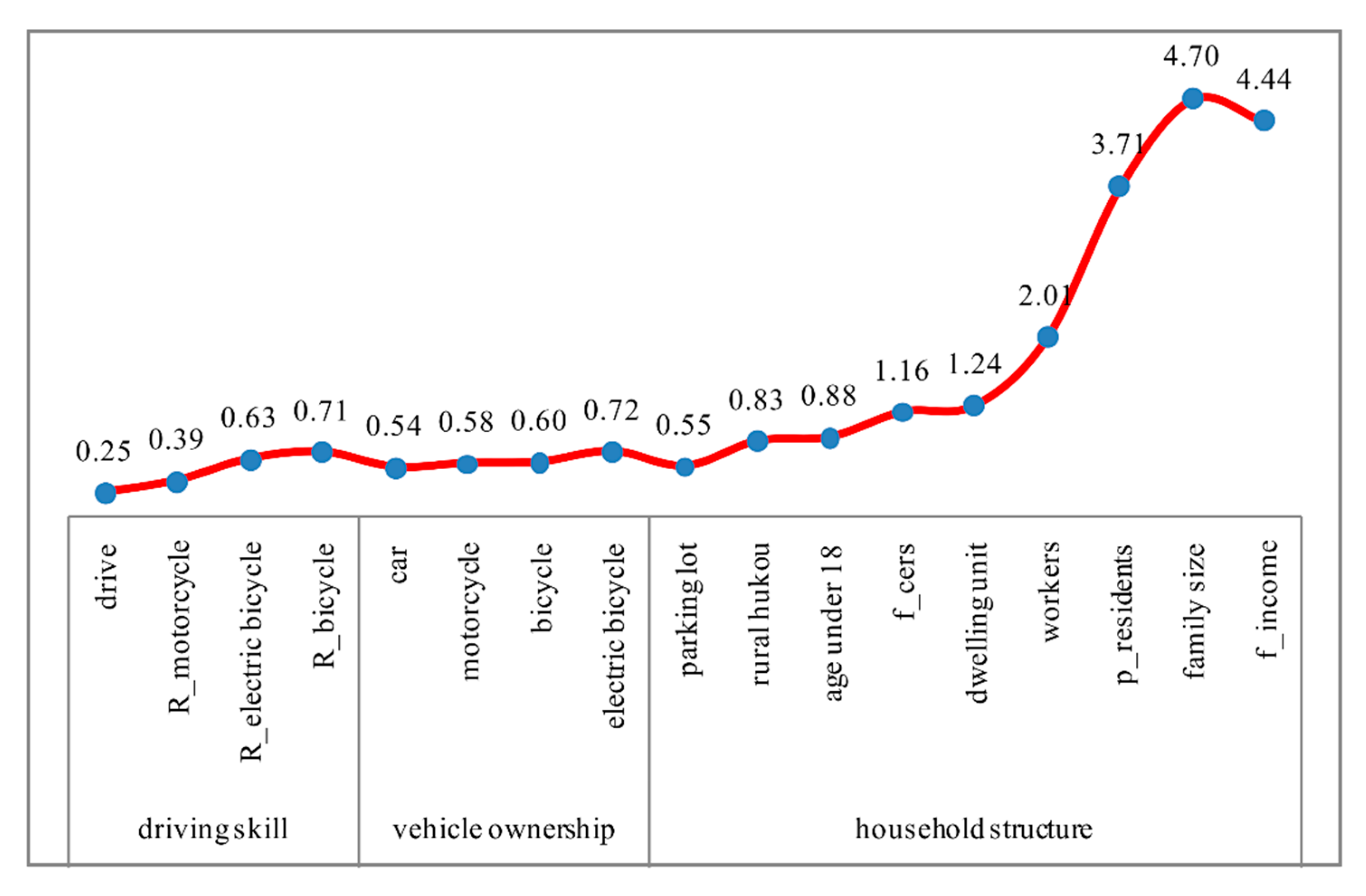
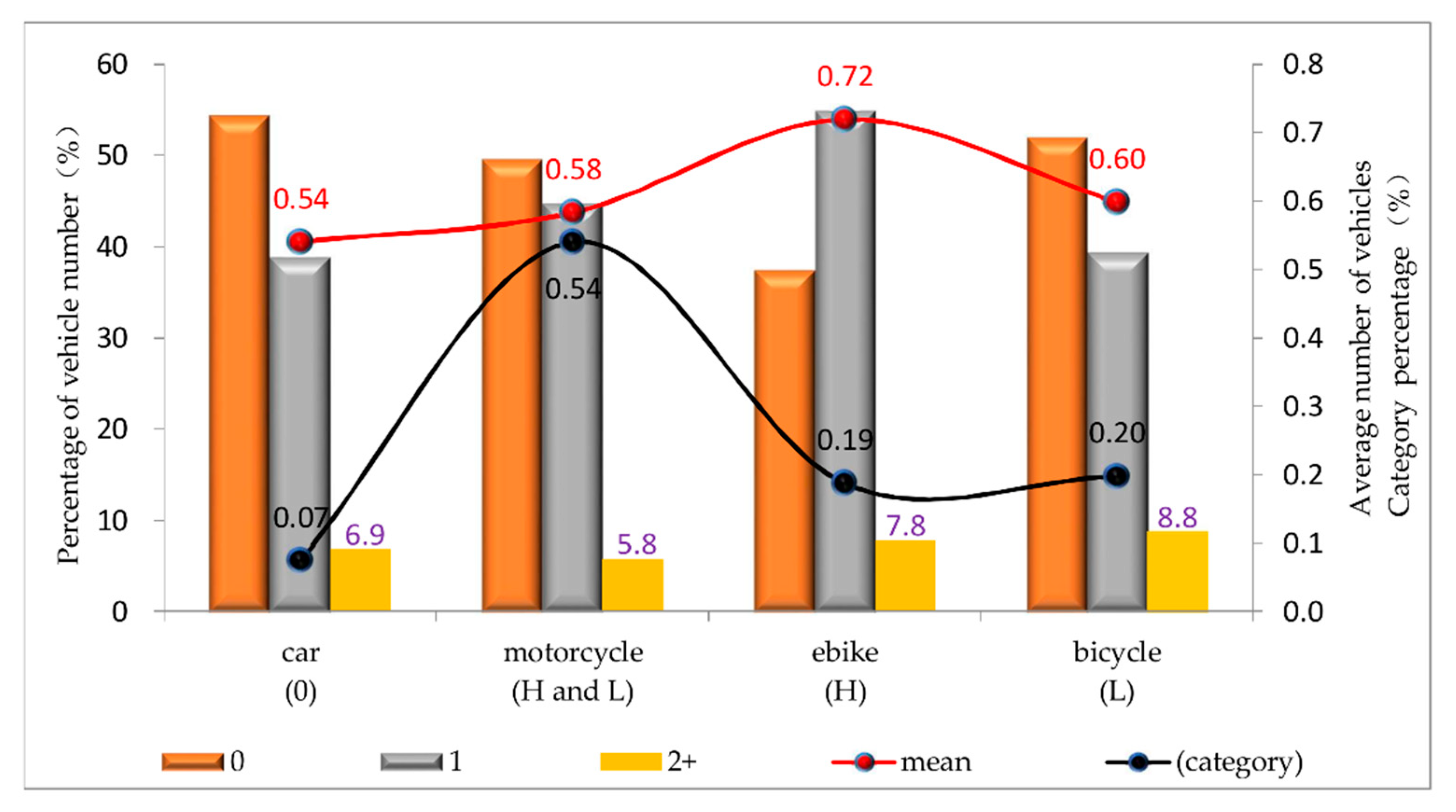
Respondent characteristics, including driving skills, household vehicle ownership, and household structure, are summarized in Figure 4. Of the respondents, 25% had a driver’s license. The percentage of respondents who could ride a motorcycle, electronic bicycle, and bicycle was 39%, 63%, and 71%, respectively. The average number of cars, motorcycles, bicycles, and electronic bicycles per household was0.54, 0.58, 0.60, and 0.72, respectively. Of all the respondents, 83% were rural hukou. Other information about household structure attributes are shown in Figure 4.

3.3. Measurement of Rural Built Environment

The rural built environment is different from the urban built environment in China. Thus, we regulated the scope of measurement by considering the living style of the sample village residents when measuring the built environment indicators. (1) The scope for calculating the built environment indicators was a circle with a 1 km radius from the village center (village committee or neighborhood committee office) for Huojing and Dongxing villages. Although the respondents from Shangteng also had a centralized living style, Shangteng is a new rural village under construction, thus the village possesses many characteristics of a scattered-living village. (2) The administrative village boundary is the scope for calculating the built environment indicators in scattered-living traditional villages. The main reason for this is that the administrative areas of scattered-living traditional villages in Sichuan Province vary considerably and the degree of decentralization is inconsistent. The surveyed households were not completely within the scope of the 1 km circle.
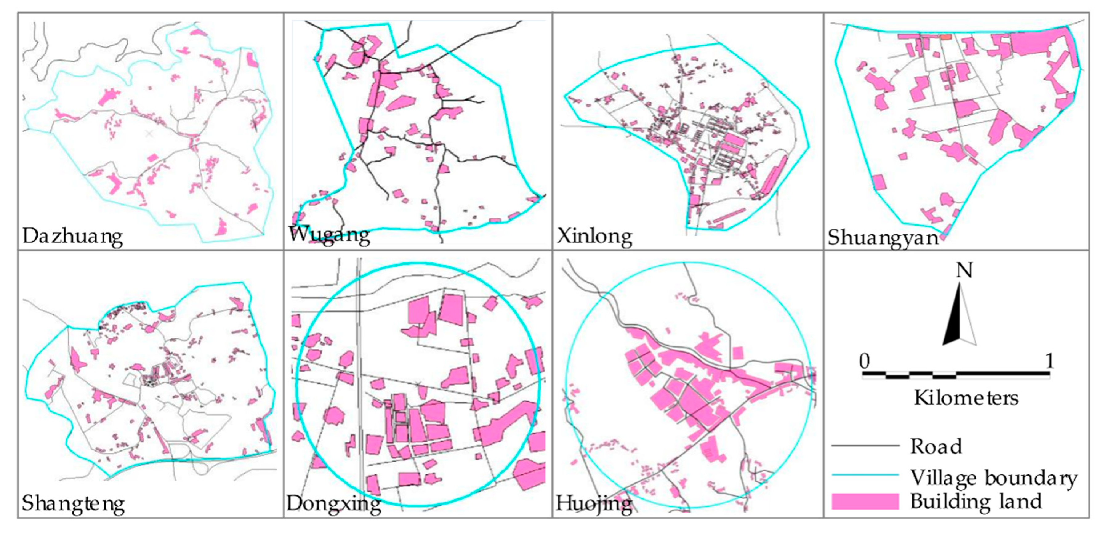
We mainly used two approaches to obtain basic data of the actual built environment considering the limited geographical information of rural areas in China. First, the researchers conducted an on-site measurement using the Baidu navigation app to search and measure the distance to the nearest bus station, train station, bus stop, main road, market, school, health center (hospital), and center of the city (county) from the village center. The basic data measured onsite are shown in Table 3. Second, the basic data of buildings and roads were coded from Tencent street view imagery (map.qq.com) using ArcGIS 10.2. The road and building land information from ArcGIS 10.2 is shown in Figure 5.

4. Methods

4.1. Variable Specification

4.1.1. Dependent Variables

In the basic statistical analysis, most of the households owned zero or one car, motorcycle, electric bicycle, and/or bicycle in the sample rural villages. Only 6.9%, 5.8%, 7.8%, and 8.8% of the households owned two or more cars, motorcycles, electric bicycles, and/or bicycles, respectively. Therefore, the households were classified into two groups: with or without a certain vehicle. In addition, electric bicycles and bicycles were considered as low-carbon vehicles, whereas motorcycles and cars were classified as high-carbon vehicles. This classification was based on the vehicle’s power source and carbon emission level. Finally, the rural household vehicle ownership combination set was no vehicles, only low-carbon vehicles, only high-carbon vehicles, and high- and low-carbon vehicles, which is denoted by {0, L, H, H&L}. Additional information about household vehicle ownership from the sample villages is shown in Figure 6.

4.1.2. Socio Demographic Variables

Socio demographic characteristics affect household vehicle ownership decisions. Thus, we also collected information about the respondents and their households. In this study, household structure attributes and respondents’ driving skills were selected as the main variables because of their significant effects on vehicle ownership. These variables include the numbers of permanent residents, workers, household members under 18, driver’s license holders, dwelling units, household parking lots, and rural hukou; household income; and respondents’ ability to operate vehicles such as cars, motorcycles, electric bicycles, and bicycles.
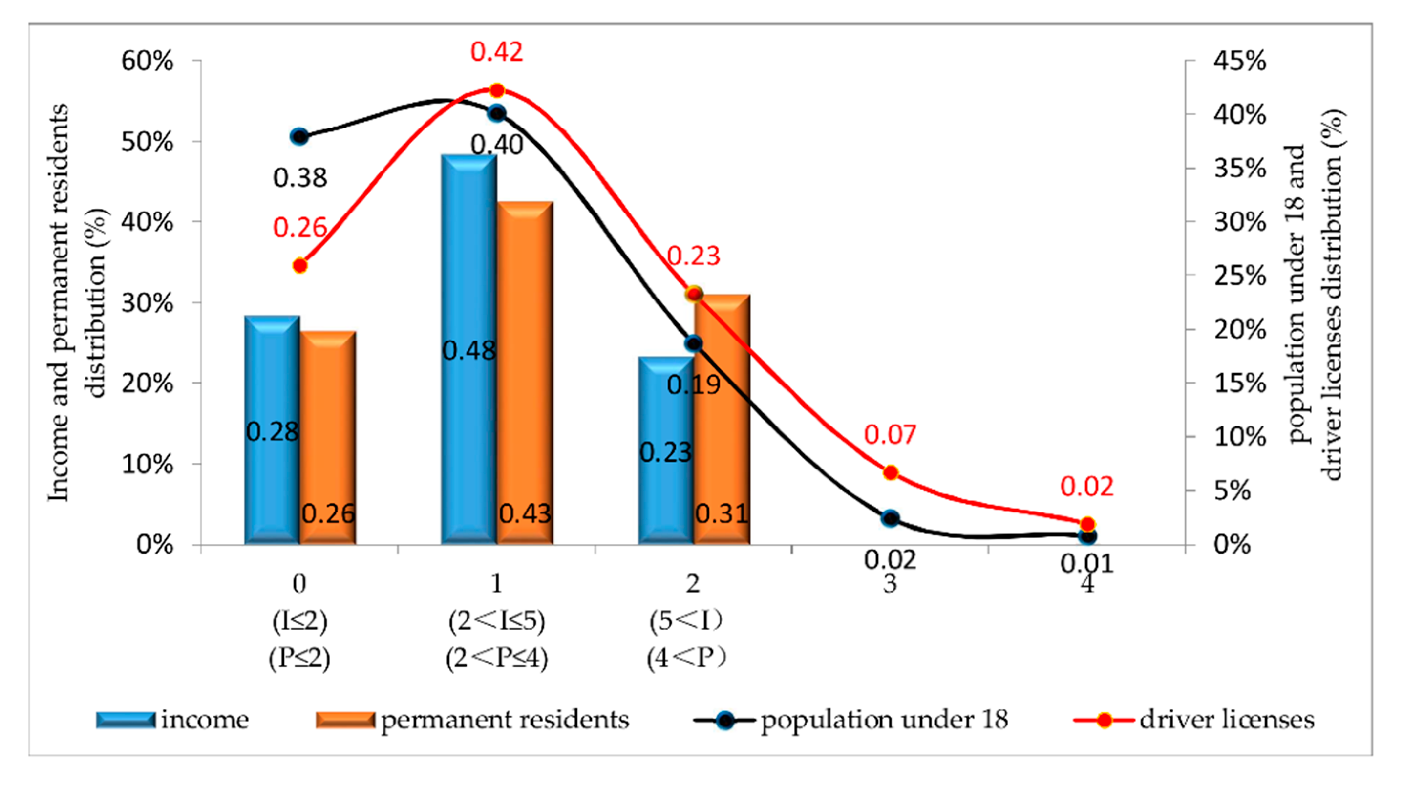
Household size, number of household members under 18, household income, and number of driver’s license holders always significantly influenced vehicle ownership. Thus, we coded these four as dummy variables based on the basic statistical analysis results to obtain additional detailed information about the relationship between these variables and vehicle ownership. Further information about these four variables is shown in Figure 7, and descriptive statistics are shown in Table 4.

4.1.3. Built Environment Variables

Built environments in rural areas are simpler than those in cities; however, rural built environments pose more difficulties in data collection. This study is mainly concerned about the “4Ds+1S” built environment variables on the basis of on-site measurement of basic data and GIS extraction data. These variables are design, diversity, distance to transit, destination accessibility, and living style. Although we investigated the population and number of households in the sample villages, we were unable to obtain accurate data on the population and households within the 1 km radius from the central residential area. Finally, we did not consider the density variables, population density and dwelling unit density.
The study design denotes road density and is calculated as
Design index = Total length of roads (m)/Total survey area (mu)
Land-use mix is consistently used in calculating the diversity index in most of the related studies. However, land use in rural areas is relatively single, and we can only read building land by using GIS technology. Thus, in this study, building density was used to calculate the diversity of rural land use. Here, mu is a unit of land area in China. Fifteen acres equals one hectare.
Diversity index = Building land area (m2)/Total survey area (m2)
Anowar et al. [46] used mix index to calculate the distance to transit. We simplified their formula to calculate the distance-to-transit mix index and destination accessibility mix index.
Distance - to - transit   mix   index = k { 1 / ( d k + 1 ) }
where k = 1 ,   2 ,   3 ,   4 , and d k represents the distance from the village center to the nearest bus station, train station, public transportation station, and main road.
Destination   accessibility   mix   index = k { 1 / ( d k + 1 ) }
where k = 1 ,   2 ,   3 ,   4 , and d k represents the distance from the village center to the nearest market, school, health center (hospital), and city (county) center.
As a result of urbanization, the lifestyle of rural residents is gradually shifting from traditional scattered living to urbanized centralized living, and such change directly influences household decisions on vehicle ownership. Thus, aside from the influences of the D variables, the influence of living style on vehicle ownership was also investigated in this study. All the variables used in this study are shown in Table 4.
Multicollinearity problems may cause low significance levels of various spatial variables [47]. Therefore, the multicollinearity of the independent variables in this study should be examined. The variable expansion factor (VIF) was used to test for multicollinearity. A larger VIF value indicates that a particular explanatory variable is more likely to be represented by a linear function model with other explanatory variables and that the model may have multicollinearity problems [48]. Our analysis implied that the VIF values of the explanatory variables were well below 5, indicating that no multicollinearity problem was present.

4.2. Model Specification

We classified vehicle ownership into four categories: no vehicles (0), owning low-carbon vehicles (L), owning high-carbon vehicles (H), and owning high-and low-carbon vehicles (H&L). The utility functions for vehicle ownership of each household can be expressed as follows [43,49]:
U ( 0 ) = β 0 x n 0 + ε n 0
U ( L ) = β L x n L + ε n L
U ( H ) = β H x n H + ε n H
U ( H & L ) = β H & L x n H & L + ε n H & L
where y n = i i f U n ( i ) > U n ( q ) q i , and ε is assumed to be independently and identically distributed with identical extreme value distribution. The distribution function is
F ( ε i ) = e x p ( e x p ( ε i ) )
On the basis of this specification, the choice probabilities are
P r o b ( i ) = P r o b ( U n ( i ) > U n ( q ) ) = e ( β i x n i ) / q = 0 J e ( β q x n q ) ,   q i ,   i = 0 ,   L ,   H ,   H & L
i = 0 ,   L ,   H ,   H & l P r o b ( y n = i ) = 1 ,   0 P r o b ( y n = i ) 1 ,   i = 0 ,   L ,   H ,   H & L
We used the option H as a reference option. With the coefficient β H = 0 , this equation can berewritten as
P r o b ( y n = i ) = P r o b ( U n ( i ) > U n ( q ) ) = 1 / ( e ( β 0 x n 0 ) + e ( β L x n L ) + e ( β H & L x n H & L ) + 1 ) ,   i = H
P r o b ( y n = i ) = P r o b ( U n ( i ) > U n ( q ) ) = ( e β i x n i ) / ( e ( β 0 x n 0 ) + e ( β L x n L ) + e ( β H & L x n H & L ) + 1 ) ,   i = 0 ,   L ,   H & L

5. Results and Discussion

The MNL model of vehicle ownership of rural households contains all the explanatory variables described in the previous section. We used NLOGIT 5.0 for the model estimation. The explanatory variables were entered into the model one by one, following the categories of household structure attributes, respondent driving skills, and rural built environment. Likelihood ratio tests were performed. The results of these tests are summarized in Table 5. The test results show that every variable category contributes significantly to the model, because all likelihood ratio values are well above the critical value. The log-likelihood value increased from −434.20 to −269.33, thus each category variable should be included in the set of explanatory variables to explain rural household vehicle ownership. However, the relative explanatory power of each category variable cannot be observed from the results in Table 5. Accordingly, another set of likelihood ratio tests was conducted, the results of which are shown in Table 6. The household structure attributes had the highest likelihood value, which implies that this variable had the highest explanatory power among all the explanatory variables. Built environment and personal driving skill variables follow the household structure attributes.
We set high-carbon vehicles (H) as the reference option to estimate the model parameters. We specified a full set of alternative specific constants corresponding to no vehicles, low-carbon vehicles, and high- and low-carbon vehicles, and all were statistically significant. Generally, specific constants capture unobserved information [50]. In the vehicle ownership model, alternative specific constants capture the costs associated with vehicle ownership: purchase, maintenance, and lease costs [51]. The cost information of household owned vehicles is difficult to collect accurately, thus the MNL model in this study does not include specific cost variables, and the relationship between unobserved information and vehicle ownership is reflected by the specific constant items. Under the same conditions, the utility of a rural household for owning no vehicle, low-carbon vehicles, high-carbon vehicles, and high- and low-carbon vehicles is gradually reduced for the unobserved information related to cost (Table 7). This result is easy to understand and fully meets our expectations. It also agrees with the findings of Choudhary et al. [52], who categorized household vehicle ownership into no vehicles (0), two-wheeled vehicles (2W), four-wheeled vehicles (4W), and two- and four-wheeled vehicles (2&4W), in descending order0 > 2W > 4W > 2&4W.

5.1. Household Structure Attributes

Nearly all the household structure attributes that were explanatory variables, except for numbers of dwelling units and household parking lots, had a significant influence on vehicle ownership. Households with a resident population >5 had the highest utility for owning high- and low-carbon vehicles, followed by owning only low-carbon vehicles. For households with a resident population of 3–4, the negative βvalue indicates that they were more willing to own high-carbon vehicles. In addition, compared with household utility for owning only high-carbon vehicles, household utility increased significantly with an increased number of permanent residents owning high- and low-carbon vehicles, only low-carbon vehicles, and no vehicles. Households with members under the age of 18 were inclined to own high- and low-carbon vehicles; however, the utility for owning high- and low-carbon vehicles did not increase significantly with an increased number of members under 18. Households with two or more members with a driver’s license were most likely to own only high-carbon vehicles, followed by high- and low-carbon vehicles, only low-carbon vehicles, and no vehicles; and the utilities of the different vehicle ownership categories significantly differed. The probability of owning vehicles for high-income households, in descending order, was H&L > H > L > 0. All the βvalues for high-income households were statistically significant, and the significant difference indicated that the utility of high-income households with different vehicle ownership categories were significantly different. By contrast, the βvalues for middle-income households were only statistically significant for no vehicles, and negative βvalues implied lower utility of middle-income households with no vehicles than with high-carbon vehicles. This finding agrees with previous studies, which asserted that household income is the key factor influencing vehicle ownership [6,49], especially for high-income households. All three estimated parameters (β) for rural hukou were negative and only statistically significant for low-carbon vehicles, indicating that rural households with rural hukou were more willing to own high-carbon vehicles. This finding is in contrast to previous studies on car ownership in the urban Chinese context. Specifically, Yang et al. [43] studied household car ownership in Jinan and found that households with rural hukou had a relatively low probability of buying cars. However, an in-depth analysis revealed that this difference was entirely dependent on the actual conditions of urban and rural areas in China. Compared to urban residents, rural residents who worked in urban areas had lower income and fewer resources. Although some rural residents have been urbanized and their lands have been expropriated in the process of urbanization, they rely on government subsidies to live without stable work. Therefore, urbanized rural households in rural areas and rural households in urban areas had lower utility of owning automobiles and were less likely to own more automobiles. Households with several workers were willing to own high-carbon vehicles; this finding is consistent with other studies on car ownership [6,53].

5.2. Personal Skills

In addition to household structure attributes, the driving skill of respondents was considered in this study. Although the respondents’ individual characteristics demonstrated a limited effect on household vehicle ownership, variability in driving skill is directly and significantly related to vehicle ownership. Personal driving skills involved four variables: whether they had a driver’s license, and whether they could ride a motorcycle, bicycle, and/or electric bicycle. As shown in Table 7, all four variables were statistically significant. All three estimated parameters of holding a driver’s license were negative, but only statistically significant for high- and low-carbon vehicles. The β values for riding a motorcycle for low-carbon vehicles and high- and low-carbon vehicles were negative and statistically significant. These results show that people skilled at driving high-carbon vehicles were inclined to own high-carbon vehicles. In addition, people who could ride a motorcycle had the lowest utility for owning low-carbon vehicles. This outcome demonstrates that motorcycles are deemed to have the kinetic energy of automobiles and the convenience of low-carbon vehicles. The estimated parameters of cycling and riding an electric bicycle were relatively consistent. For households that owned high- and low-carbon vehicles, both cycling and riding an electric bicycle had nearly the same positiveβ coefficient, indicating that both types of household were willing to own high- and low-carbon vehicles. By contrast, those who could ride an electric bicycle (or their household) had the highest utility to own low-carbon vehicles. However, those who could ride a bicycle (or their household) had a relatively low utility for owning low-carbon vehicles because of lower kinetic energy and convenience than electric bicycles. Thus, the ability to ride a motorcycle and/or electric bicycle had a significant influence on vehicle ownership decisions for households in rural areas.

5.3. The Built Environment

The effects of the five variables of the built environment on vehicle ownership of rural households are statistically significant. Specifically, building density, road density, and destination accessibility (distance to the nearest hospital/health center, school, market, and city/county center) had significant negative effects on owning no vehicles, indicating that with increased road density, building density, and destination accessibility in rural areas, households were more willing to own high-carbon vehicles. This result is in contrast to previous studies on household car ownership in Chinese urban areas. Building and road densities are generally believed to have a positive influence on walking activities for residents and negative influence on vehicle ownership [3,21,38,47]. Two studies indicated that a shorter distance from the CBD and job center implies lower vehicle ownership [6,9]. The main reason behind the contradicting results between the current study and previous studies is the huge gap between the rural and urban built environments in China. For Sichuan rural areas, building and road densities can represent the development level of infrastructure to some extent. Although rural areas are urbanizing rapidly, the rural built environment indicators still lag far behind cities. For example, the average building density of 20 districts in Jinan City is 0.407 [54], whereas that of the sample villages selected in this study is 0.119. In the process of rural urbanization, residents are more reluctant to have no vehicles than high-carbon vehicles as building density, road density, and destination accessibility increase. As shown in Table 7, destination accessibility had the largest influence on owning no vehicles, followed by road and building densities. Therefore, walking- or cycling-oriented rural planning could effectively reduce rural automobile ownership and vehicle carbon emissions. Locations of schools and health centers should be planned within walking and riding range for rural residents. In addition, building density and distance to transit positively influence downing high- and low-carbon vehicles, with distance to transit having a greater influence. Finally, the centralized living style had a significant positive effect on owning no vehicles, high- and low-carbon vehicles, and low-carbon vehicles, although the degree of influence weakened, in the stated order. This is consistent with our expectation that rural households with a centralized living style are more willing to own no vehicles, high- and low-carbon vehicles, or low-carbon vehicles than high-carbon vehicles. In the process of rural urbanization, the living style of households changes from traditional scattered living to urbanized centralized living, and the spatial distance between neighborhoods gradually shrinks. Although centralized living areas have the characteristics of a city and the comprehensive service level in these areas is higher than that in traditional scattered residential areas, a certain gap exists between the two living styles in the level of urban development. Thus, walking can meet the need for basic neighborhood interactions; however, important destinations, such as schools, hospitals/health centers, and bazaars, are still outside the walking distance. Finally, no vehicles and high- and low-carbon vehicles had the highest probabilities of being selected for centralized-living rural households.
In the estimation of the standardized parameters of all variables, household structure variables had the most significant influence on rural household vehicle ownership. This result is consistent with existing research findings [55,56]. The household structure variables were followed by built environment variables, indicating that the rapid and considerable changes in rural built environment have a significant effect on household vehicle ownership in rural China.

6. Conclusions and Policy Implications

With the rapid rural urbanization and new construction in rural China, tremendous changes are occurring, along with a considerable increase in the energy consumption of rural households. One of the key factors is the change in rural household vehicle ownership. The use of GIS technology and a discrete choice model allows scholars to investigate the relationship between built environment and household vehicle ownership.
This study is one of the first to investigate household vehicle ownership in the rural built environment context. The MNL model of vehicle ownership was derived from data collected through a rural village and household survey and with the use of GIS technology.
The results show that all household structure attributes, personal skills, and rural built environment variables have a significant influence on household vehicle ownership. The likelihood ratio tests also show that the built environment variables similarly have great effects. All these findings can help rural policy-makers and planners create effective policies and design potential interventions by considering personal driving skills and the rural built environment. To reduce travel energy consumption and carbon emissions, we suggest the following: (1) Important destinations, such as schools, hospitals/health centers, and bazaars, should be planned such that they are within walking and cycling distance. (2) In the process of urbanization, a reasonable scale of centralized residential areas should be established for urbanized rural households. (3) Rural residents should be encouraged to learn to ride bicycles and electric bicycles. (4) Rural residents also should be encouraged to learn to ride motorcycles, which can lead to a reduction in household car ownership.
Some possible future research opportunities could include: (1) exploring the effects of the rural built environment on rural individuals’ mode choice (including long and short distances); (2) testing the influence of fast changes in the rural built environment on rural residents’ travel behavior and/or activities; (3) considering the interaction among individual self-selection, the rural built environment, vehicle ownership, and travel activities; and (4) incorporating more rural built environments to test the spatial heterogeneity in rural China.

Author Contributions

All authors contributed to the research presented in this paper. C.C., Y.A., and D.Y. had the original idea for the study; the co-authors conceived and designed the questionnaire. Y.A. and Y.W. organized the investigation; Y.A. analyzed the data and drafted the manuscript, which was revised by C.C., D.Y., and Y.W. All authors have read and approved the final manuscript.

Acknowledgments

The authors appreciate financial support from (Jian Qi 666) Promoting the Cooperation 24 between the Government of Sichuan Province and Social Capital (0050205502123), the Fundamental Research Funds for the Central Universities (2012017yjsy215), the Natural Science Key Project from the Sichuan Provincial Department of Education (18ZA0048), the Fundamental Philosophy and Social Science Research Fund for Chengdu University of Technology (YJ2017-NS011), the Research on BIM Technology Resource Sharing Platform Construction and Cooperation Mechanism (CHJK{2017}119), and the Development Research Center of Oil and Gas, Sichuan (CYQK-SKB17-04).

Conflicts of Interest

The authors declare no conflict of interest.

References

  1. National Bureau of Statistics. China Statistical Yearbook. 1986–2017. Available online: http://tongji.cnki.net/kns55/Navi/HomePage.aspx?id=N2017100312&name=YINFN&floor=1 (accessed on 28 Janurary 2018).
  2. Wang, D.; Chai, Y.; Li, F. Built environment diversities and activity–travel behaviour variations in Beijing, China. J. Transp. Geogr. 2011, 19, 1173–1186. [Google Scholar] [CrossRef]
  3. Li, S.; Zhao, P. Exploring car ownership and car use in neighborhoods near metro stations in Beijing: Does the neighborhood built environment matter? Transp. Res. Part D Transp. Environ. 2017, 56, 1–17. [Google Scholar] [CrossRef]
  4. Ministry of Environment Protection. 2015 Annual Report of Automobile Air Pollution in China; Protection, M.O.E., Ed.; Ministry of Environment Protection: Beijing, China, 2016.
  5. Handy, S.; Cao, X.; Mokhtarian, P. Correlation or causality between the built environment and travel behavior? Evidence from Northern California. Transp. Res. Part D Transp. Environ. 2005, 10, 427–444. [Google Scholar] [CrossRef]
  6. Potoglou, D.; Kanaroglou, P.S. Modelling car ownership in urban areas: A case study of Hamilton, Canada. J. Transp. Geogr. 2008, 16, 42–54. [Google Scholar] [CrossRef]
  7. Vance, C.; Hedel, R. The impact of urban form on automobile travel: Disentangling causation from correlation. Transportation 2007, 34, 575–588. [Google Scholar] [CrossRef]
  8. Ewing, R.; Tian, G.; Goates, J.P.; Zhang, M.; Greenwald, M.J.; Joyce, A.; Kircher, J.; Greene, W. Varying influences of the built environment on household travel in 15 diverse regions of the United States. Urban Stud. 2015, 52, 2330–2348. [Google Scholar] [CrossRef]
  9. Ewing, R.; Cervero, R. Travel and the Built Environment. J. Am. Plan. Assoc. 2010, 76, 265–294. [Google Scholar] [CrossRef]
  10. Ewing, R.; Cervero, R. Travel and the built environment—A synthesis. Transp. Res. Rec. J. Transp. Res. Board 2001, 1780, 87–114. [Google Scholar] [CrossRef]
  11. Ewing, R.; Handy, S. Measuring the Unmeasurable: Urban Design Qualities Related to Walkability. J. Urban Des. 2009, 14, 65–84. [Google Scholar] [CrossRef]
  12. Zhang, Y.; Wu, W.; Li, Y.; Liu, Q.X.; Li, C.Y. Does the Built Environment Make a Difference? An Investigation of Household Vehicle Use in Zhongshan Metropolitan Area, China. Sustainability 2014, 6, 4910–4930. [Google Scholar] [CrossRef]
  13. Wang, Y.; Peng, Z.; Wang, K.; Song, X.; Yao, B.; Feng, T. Research on Urban Road Congestion Pricing Strategy Considering Carbon Dioxide Emissions. Sustainability 2015, 7, 10534–10553. [Google Scholar] [CrossRef]
  14. Broberg, A.; Sarjala, S. School travel mode choice and the characteristics of the urban built environment: The case of Helsinki, Finland. Transp. Policy 2015, 37, 1–10. [Google Scholar] [CrossRef]
  15. Cao, X.; Mokhtarian, P.L.; Handy, S.L. The relationship between the built environment and nonwork travel: A case study of Northern California. Transp. Res Part A Policy Pract. 2009, 43, 548–559. [Google Scholar] [CrossRef]
  16. Stewart, O.T.; Moudon, A.V. Using the built environment to oversample walk, transit, and bicycle travel. Transp. Res. Part D Transp. Environ. 2014, 32, 15–23. [Google Scholar] [CrossRef]
  17. Zhao, P.J. The Impact of the Built Environment on Bicycle Commuting: Evidence from Beijing. Urban Stud. 2014, 51, 1019–1037. [Google Scholar] [CrossRef]
  18. Feng, J.X. The influence of built environment on travel behavior of the elderly in urban China. Transp. Res. Part D Transp. Environ. 2017, 52, 619–633. [Google Scholar] [CrossRef]
  19. Hess, D.B.; Ong, P.M. Traditional neighborhoods and automobile ownership. Transp. Res. Rec. J. Transp. Res. Board 2002, 1805, 35–44. [Google Scholar] [CrossRef]
  20. Van Acker, V.; Witlox, F. Car ownership as a mediating variable in car travel behaviour research using a structural equation modelling approach to identify its dual relationship. J. Transp. Geogr. 2010, 18, 65–74. [Google Scholar] [CrossRef] [Green Version]
  21. Zegras, C. The Built Environment and Motor Vehicle Ownership and Use: Evidence from Santiago de Chile. Urban Stud. 2010, 47, 1793–1817. [Google Scholar] [CrossRef]
  22. Chatman, D.G. Does TOD Need the T? On the Importance of Factors Other Than Rail Access. J. Am. Plan. Assoc. 2013, 79, 17–31. [Google Scholar] [CrossRef]
  23. Keller, R.; Vance, C. Landscape pattern and car use: Linking household data with satellite imagery. J. Transp. Geogr. 2013, 33, 250–257. [Google Scholar] [CrossRef]
  24. Cervero, R. Mixed land-uses and commuting: Evidence from the American housing survey. Transp. Res Part A Policy Pract. 1996, 30, 361–377. [Google Scholar] [CrossRef]
  25. Hong, J.H.; Shen, Q.; Zhang, L. How do built-environment factors affect travel behavior? A spatial analysis at different geographic scales. Transportation 2014, 41, 419–440. [Google Scholar] [CrossRef]
  26. Holtzclaw, J.; Clear, R.; Dittmar, H.; Goldstein, D.; Haas, P. Location efficiency: Neighborhood and socioeconomic characteristics determine auto ownership and use—Studies in Chicago, Los Angeles and San Francisco. Transp. Plan. Technol. 2002, 25, 1–27. [Google Scholar] [CrossRef]
  27. McCormack, E.; Rutherford, G.S.; Wilkinson, M.G. Travel impacts of mixed land use neighborhoods in Seattle, Washington. Transp. Res. Rec. J. Transp. Res. Board 2001, 1780, 25–32. [Google Scholar] [CrossRef]
  28. Krizek, K.J. Residential relocation and changes in urban travel—Does neighborhood-scale urban form matter? J. Am. Plan. Assoc. 2003, 69, 265–281. [Google Scholar] [CrossRef]
  29. Miller, E.J.; Ibrahim, A. Urban form and vehicular travel—Some empirical findings. Transp. Res. Rec. J. Transp. Res. Board 1998, 1617, 18–27. [Google Scholar] [CrossRef]
  30. Cervero, R.; Arrington, G.B. Vehicle Trip Reduction Impacts of Transit-Oriented Housing. J. Public Transp. 2008, 11, 1–17. [Google Scholar] [CrossRef]
  31. Guo, Z. Does residential parking supply affect household car ownership? The case of New York City. J. Transp. Geogr. 2013, 26, 18–28. [Google Scholar] [CrossRef]
  32. Tyrinopoulos, Y.; Antoniou, C. Factors affecting modal choice in urban mobility. Eur. Transp. Res. Rev. 2013, 5, 27–39. [Google Scholar] [CrossRef]
  33. Chatman, D.G. Deconstructing development density: Quality, quantity and price effects on household non-work travel. Transp. Res Part A Policy Pract. 2008, 42, 1008–1030. [Google Scholar] [CrossRef]
  34. Cameron, I.; Kenworthy, J.R.; Lyons, T.J. Understanding and predicting private motorised urban mobility. Transp. Res. Part D Transp. Environ. 2003, 8, 267–283. [Google Scholar] [CrossRef]
  35. Lee, C.-K.; Shaw, M.-S. Constrained Diffusion Models for the Prediction of Multi-Class Motor Vehicle Ownership. Volume 1: Travel Behavior. In Proceedings of the 7th World Conference on Transport ResearchWorld Conference on Transport Research Society, Sydney, Australia, 16–21 July 1996. [Google Scholar]
  36. Lin, C.-Y.; Liao, Y. Perceptions of activity-supportive environment and motorcycle use among urban Taiwanese adults. BMC Public Health 2017, 17, 665. [Google Scholar] [CrossRef] [PubMed]
  37. Oyedepo, O.J.; Etu, J. Binomial logistic regression model of household motorcycle ownership in Akure, Ondo State, Nigeria. J. Transp. Lit. 2015, 9, 40–44. [Google Scholar] [CrossRef]
  38. Bhat, C.R.; Guo, J.Y. A comprehensive analysis of built environment characteristics on household residential choice and auto ownership levels. Transp. Res. Part B Methodol. 2007, 41, 506–526. [Google Scholar] [CrossRef]
  39. Cao, J.S.; Cao, X.S. The Impacts of LRT, Neighbourhood Characteristics, and Self-selection on Auto Ownership: Evidence from Minneapolis-St. Paul. Urban Stud. 2014, 51, 2068–2087. [Google Scholar] [CrossRef]
  40. Zhao, Y.; Chai, Y. Residents’ activity-travel behavior variation by communities in Beijing, China. Chin. Geogr. Sci. 2013, 23, 492–505. [Google Scholar] [CrossRef]
  41. Cheng, T.J.; Selden, M. The Origins And Social-Consequences of China Hukou System. China Q. 1994, 139, 644–668. [Google Scholar] [CrossRef]
  42. Zhao, P. Car use, commuting and urban form in a rapidly growing city: Evidence from Beijing. Transp. Plan. Technol. 2011, 34, 509–527. [Google Scholar] [CrossRef]
  43. Jiang, Y.; Gu, P.; Chen, Y.; He, D.; Mao, Q. Influence of land use and street characteristics on car ownership and use: Evidence from Jinan, China. Transp. Res. Part D Transp. Environ. 2017, 52, 518–534. [Google Scholar] [CrossRef]
  44. Feng, J.X.; Dijst, M.; Wissink, B.; Prillwitz, J. Understanding Mode Choice in the Chinese Context: The Case of Nanjing Metropolitan Area. Tijdschr. Voor Econ. Soc. Geogr. 2014, 105, 315–330. [Google Scholar] [CrossRef]
  45. Zhang, Y.; Yang, X.; Li, Y.; Liu, Q.; Li, C. Household, Personal and Environmental Correlates of Rural Elderly’s Cycling Activity: Evidence from Zhongshan Metropolitan Area, China. Sustainability 2014, 6, 3599–3614. [Google Scholar] [CrossRef]
  46. Anowar, S.; Yasmin, S.; Eluru, N.; Miranda-Moreno, L.F. Analyzing car ownership in Quebec City: A comparison of traditional and latent class ordered and unordered models. Transportation 2014, 41, 1013–1039. [Google Scholar] [CrossRef]
  47. Ding, C.; Wang, D.; Liu, C.; Zhang, Y.; Yang, J. Exploring the influence of built environment on travel mode choice considering the mediating effects of car ownership and travel distance. Transp. Res. Part A Policy Pract. 2017, 100, 65–80. [Google Scholar] [CrossRef]
  48. Yao, B.; Hu, P.; Lu, X.; Gao, J.; Zhang, M. Transit network design based on travel time reliability. Transp. Res. Part C Emerg. Technol. 2014, 43, 233–248. [Google Scholar] [CrossRef]
  49. Train, K.E. Discrete Choice Methods with Simulation; Cambridge University Press: Cambridge, UK, 2009. [Google Scholar]
  50. Moshe, B.-A.; Lerman, S. Discrete Choice Analysis: Theory and Application to Travel Demand; Massachusetts Institute of Technology: Cambridge, MA, USA, 1985. [Google Scholar]
  51. Ryan, J.; Han, G. Vehicle-ownership model using family structure and accessibility application to Honolulu, Hawaii. Transp. Res. Rec. J. Transp. Res. Board 1999, 1676, 1–10. [Google Scholar] [CrossRef]
  52. Choudhary, R.; Vasudevan, V. Study of vehicle ownership for urban and rural households in India. J. Transp. Geogr. 2017, 58, 52–58. [Google Scholar] [CrossRef]
  53. Hirota, K. Comparative Studies on Vehicle Related Policies for Air Pollution Reduction in Ten Asian Countries. Sustainability 2010, 2, 145–162. [Google Scholar] [CrossRef]
  54. Yang, Y. A Research on Neighborhood Built Environment and Household Travel Energy Consumption in Jinan. Ph.D. Thesis, Tsinghua University, Beijing, China, 2013. [Google Scholar]
  55. He, S.Y.; Thøgersen, J. The impact of attitudes and perceptions on travel mode choice and car ownership in a Chinese megacity: The case of Guangzhou. Res. Transp. Econ. 2017, 62, 57–67. [Google Scholar] [CrossRef]
  56. Cullinane, S. Hong Kong’s low car dependence: Lessons and prospects. J. Transp. Geogr. 2003, 11, 25–35. [Google Scholar] [CrossRef]
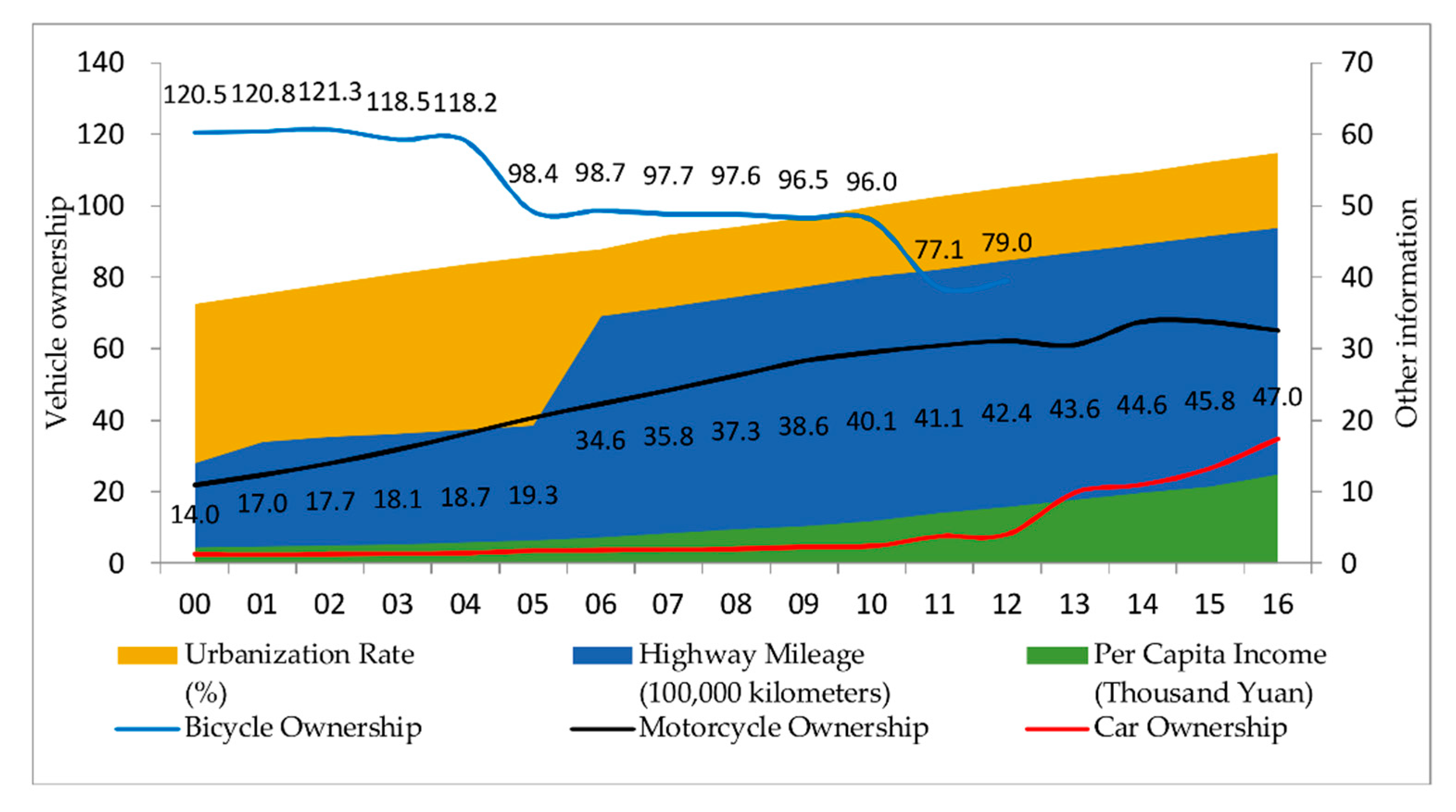
Figure 1. Household vehicle ownership and related information in rural China.
Sustainability 10 01566 g001
Figure 2. Household vehicle ownership and related information in rural Sichuan.
Sustainability 10 01566 g002
Figure 3. Built environment, regional location, and number of valid questionnaires of the sample villages.
Sustainability 10 01566 g003
Figure 4. Average values of socio demographic information.
Sustainability 10 01566 g004
Figure 5. Road and building land information.
Sustainability 10 01566 g005
Figure 6. Household vehicle ownership of the sample villages. Mean refers to average number of household vehicles; category refers to the set no vehicles, only low-carbon vehicles, only high-carbon vehicles, and high- and low-carbon vehicles {0, L, H, H&L}.
Sustainability 10 01566 g006
Figure 7. Distribution of the main socio demographic variables. I refers to household income (10,000 yuan); P refers to number of permanent residents.
Sustainability 10 01566 g007
Table 1. The commonly used indicators of “6Ds” of built environment variables.
6DsMeaningsCommonly Used Indicators
DensityVariable of interest per unit of areaDwelling unit density, employment density, population density, business density, job density
DiversityNumber of different land uses in a given area and degree to which they are representedLand-use mix (entropy index), jobs-population balance, jobs-housing balance
DesignStreet network characteristics within an areaIntersection density, street density, street connectivity, % four-way intersections
Destination accessibilityEase of access to destinationJob accessibility, distance to central business district (CBD), distance to other destinations
Distance to transitLevel of transit service at residences or workplacesDistance to bus stop, distance to rail station, distance to highway exit/subway station, bus stop density, walk minutes to transit
Demand managementResidential parking distance, quantity, or parking service levelAvg. price daily parking and hourly parking
Table 2. Sample vs. population characteristics.
Demographic Characteristics Household aVillage aRural Sichuan bRural China b
Total population
(Total permanent residents)
1758
(1388)
16,953419.6
2016: billion
5897.3
2016: billion
Total number of households3745888
Average permanent residents3.712.883.03 (2015)3.88 (2012)
Per capita income (10 k yuan)1.361.13 (2016)1.24 (2016)
Average household income (10 k yuan)4.44
Average number of household cars0.540.13 (2016)0.17 (2016)
Average number of household autobikes0.580.50 (2016)0.65 (2016)
Average number of household ebikes0.710.27 (2016)0.58 (2016)
Average number of household bicycles0.590.31 (2012)0.79 (2012)
a Data from face-to-face household survey between 29 December 2017, and 5 January 2018; b Source: China Statistical Yearbook (2013, 2016, and 2017).
Table 3. The basic data measured onsite (in km).
VillageBus StationTrain StationPublic Transport StationMain RoadMarketSchoolHealth Center (Hospital)City Center
Dazhuang18.2019.902.502.503.000.500.0519.60
Wugang0.2070.0016.000.003.502.500.2016.00
Shuangyan16.3013.400.500.501.601.600.6013.50
Xinlong13.4013.401.200.800.803.004.904.90
Dongxing3.9016.403.900.500.002.100.0010.00
Shangteng22.4024.800.690.691.501.501.6014.00
Yanjing0.50125.0034.000.501.500.501.7035.00
Table 4. Definitions and descriptive statistics of variables used in this study.
VariableDescriptionTypeMeanS.D.MinMax
Dependent variable
Vehicle ownershipNo vehicle, low-carbon vehicle, high-carbon vehicle, both low and high-carbon vehiclesCategory
Explanatory variables
Household structure
Resident population: ≥51 if household resident population is 5 or more; 0 otherwiseDummy0.310.460.001.00
Resident population: 3–41 if household resident population is 3 or 4; 0 otherwiseDummy0.430.500.001.00
Population under 18:11 if household has one member younger than 18 years of age; 0 otherwiseDummy0.400.490.001.00
Population under 18: ≥21 if household has two or more members younger than 18 years of age; 0 otherwiseDummy0.220.410.001.00
Number of license holders: 11 if number of license holders in the household is 1; 0 otherwiseDummy0.420.490.001.00
Number of license holders: ≥21 if number of license holders in the household is two or more; 0 otherwiseDummy0.320.470.001.00
Household income: high1 if income of household is more than RMB 50,000; 0 otherwiseDummy0.230.420.001.00
Household income: medium1 if income of household is between RMB 2000 and 50,000; 0 otherwiseDummy0.480.500.001.00
Household parking lot1 if household has parking lot; 0 otherwiseDummy0.540.500.001.00
Rural hukou1 if household is rural hukou; 0 otherwiseDummy0.830.370.001.00
Number of workersNumber of household workers between 18 and 65 years of ageOrdinal2.011.230.0011.00
Dwelling unitsNumber of housing unitsOrdinal1.200.540.003.00
Personal skills
Hold a driver’s license1 if respondent has a driver’s license; 0 otherwiseDummy0.250.440.001.00
Ride a motorcycle1 if respondent can ride a motorcycle; 0 otherwiseDummy0.390.490.001.00
Ride anebike1 if respondent can ride an ebike; 0 otherwiseDummy0.710.450.001.00
Ride a bicycle1 if respondent can ride a bicycle; 0 otherwiseDummy0.630.480.001.00
Built environment
Building densityDefined in Equation (1)Continuous11.815.604.7619.5
Road densityDefined in Equation (2)Continuous3.330.762.254.74
Distance to transitDefined in Equation (3)Continuous1.270.360.671.91
Destination accessibilityDefined in Equation (4)Continuous1.590.421.142.41
Living style1 if household is in concentrated area; 0 otherwiseDummy0.390.490.001.00
Table 5. Likelihood ratio index (LRI) test results: addition of explanatory variables.
KLog-Likelihood L(i)LRICritical Value *
Specific constant3L(c) = −434.20 11.345
Household structure39L(1) = −340.37−2[L(c) − L(1)] = 187.6762.428
Driving skills51L(2) = −302.98−2[L(1) − L(2)] = 74.7930.578
Built environment66L(3) = −269.33−2[L(2) − L(3)] = 67.2934.805
* Represents 0.01 significance level.
Table 6. Likelihood ratio index (LRI) test results: introduction of single explanatory variables.
KLog-Likelihood L(i)LRICritical Value *
Specific constant3L(c) = −434.20 11.345
Household structure39L(1) = −340.37−2[L(c) − L(1)] = 187.6762.428
Driving skills15L(2) = −385.99−2[L(c) − L(2)] = 96.4230.578
Built environment18L(3) = −374.47−2[L(c) − L(3)] = 119.4834.805
* Represents 0.01 significance level.
Table 7. Multinomial logit (MNL) estimated parameters of rural household vehicle ownership.
VariableH0LH&L
CoefficientPSigCoefficientPSigCoefficientPSig
Household structural attributes
Specific constant13.0080.006***3.9430.083*−4.0430.044**
Resident population: ≥50.4070.712 1.2020.063*1.5360.007***
Resident population: 3–4−1.7020.041**−0.3670.462 0.5130.262
Population under 18:11.0900.172 0.5220.294 1.0000.024**
Population under 18: ≥2−1.6210.243 0.0630.916 1.0380.044**
Number of license holders: 1−1.1940.172 0.0800.877 0.3830.447
Number of license holders: ≥2−3.4280.023**−1.4400.040**−0.1950.745
Household income: high−2.3610.062*−1.5520.029**1.2060.010**
Household income: medium−1.6850.041**−0.2080.668 0.6140.273
Household parking lot−0.9640.260 0.0930.843 0.0890.833
Rural hukou−0.3950.771 −1.3590.053*−0.8050.219
Number of workers−0.0510.895 −0.5000.017**−0.0710.647
Dwelling units−1.8750.100 −0.4380.397 0.2340.536
Personal skills
Hold a driver’s license−0.2410.851 −0.9240.144 −1.4850.004***
Ride a motorcycle0.3630.749 −1.9790.001***−1.4390.007***
Ride a bicycle−0.6950.523 0.3410.558 1.8350.002***
Ride an ebike−0.3830.779 2.2290.001***1.8350.002***
Built environment
Building density−0.0030.071*0.1080.132 0.1750.005***
Road density−1.3320.092*−0.2890.568 −0.5800.176
Destination accessibility−3.2150.091*−0.9080.318 −0.0790.921
Distance to transit mix index−2.7090.355 −0.5460.489 1.6250.007***
Living style2.5830.021**1.4400.009***1.6790.001***
Related statistics
Number of observation374
Log-likelihood with alternate specific constants(L(C))−434.204
Log-likelihood model(L(β))−269.332
Likelihood ratio = −2[L(c) − L(β)]329.745
Rho-squared (R2 = 1 − [L(β)/L(c)])0.380
Adjusted rho-squared (Adj-R2 = 1 − [(L(β) − M)/L(c)])0.330
* Significant at 10% level, ** Significant at 5% level, *** Significant at 1% level.