Article

Forest-Cover Increase Does Not Trigger Forest-Fragmentation Decrease: Case Study from the Polish Carpathians

1
Institute of Geography and Spatial Management, Jagiellonian University in Kraków, Gronostajowa 7, 30-387 Kraków, Poland
2
Institute of Environmental Sciences, Jagiellonian University in Kraków; Gronostajowa 7, 30-387 Kraków, Poland
3
Joint Research Centre, European Commission; Via Enrico Fermi 2749, I-21027 Ispra (VA), Italy, [email protected]
*
Author to whom correspondence should be addressed.
Sustainability 2018, 10(5), 1472; https://doi.org/10.3390/su10051472
Submission received: 12 April 2018 / Revised: 30 April 2018 / Accepted: 4 May 2018 / Published: 8 May 2018

Abstract

:
Understanding the causes and consequences of forest-fragmentation changes is critical for preserving various ecosystem services and to maintain biodiversity levels. We used long-term (1860s–2010s) and large-scale data on historical forest cover in the Polish Carpathians to identify the trajectories of forest fragmentation. Past forest cover was reconstructed for the 1860s, 1930s, 1970s and 2010s using historical maps and the contemporary national database of topographic objects. We analyzed forest-cover changes in 127 randomly selected circular test areas. Forest fragmentation was quantified with GuidosToolbox software using measures based on a landscape hypsometric curve (LHC). Despite a general increase in forest cover, forest fragmentation showed divergent trajectories: a decrease between the 1860s and 1930s (in 57% of test areas), and an increase between the 1930s and 1970s and between the 1970s and 2010s (in 58% and 72% of test areas, respectively). Although deforestation typically involves the increasing fragmentation of forest habitats, we found that forest expansion may not necessarily lead to more homogenous forested landscape, due to complex land-ownership and land-use legacy patterns. This is both a challenge and an opportunity for policy makers to tune policies in such a way as to maintain the desired fragmentation of forest habitats.

1. Introduction

The loss of forest habitats and forest fragmentation have been extensively investigated in the last few decades [1]. Studies carried out at various scales show that forest fragmentation is critical for maintaining biodiversity levels [2,3,4] and that deforestation increases forest fragmentation by dissecting intact forest areas, isolating forest patches, and eliminating forest corridors [5,6,7,8,9,10,11,12,13,14,15,16,17,18]. The vast evidence that forest-cover decrease is linked to increasing forest fragmentation may lead to a belief that forest expansion, on the contrary, decreases forest fragmentation. Only few studies have presented a quantitative analysis of forest fragmentation in the context of increasing or relatively stable forest cover, providing, however, inconclusive evidence for both increasing [19,20,21,22] and decreasing fragmentation [23,24]. The lack of evidence on the relationship between forest cover and forest fragmentation is remarkable in the context of the recently proposed habitat amount hypothesis [25] that underlines the influence of habitat amount on species richness, questioning at the same time the role of habitat fragmentation.
Forest expansion has been recorded since the 19th century in a number of countries all over the world [26] as a result of forest transition, referred to as the reversal of decreasing forest-cover trends [27,28,29]. The reversal, however, does not need to denote a full removal of all the consequences of the former forest-cover reduction—in particular those referring to the increased fragmentation and loss of connectivity of forested habitats. In Europe, forest transition is mostly related to the release of excess agricultural land from agricultural production (land abandonment) in marginal locations and natural secondary forest succession or afforestation [30,31,32,33,34,35,36]. Land-use legacies and persistence play a significant role as forest expansion occurs in areas with historically established settlements, infrastructural networks and land ownership, promoting some areas and excluding others from forest recovery [37,38,39]. Forest-cover increase following land abandonment is thus a slow and gradual process, in some aspects similar to the sprawl of urban areas, reproducing initial distribution of forest patches preserved in the landscape and spatial patterns of biophysical features in the landscape [40,41,42]. Contrary to deforestation that may decrease forest cover over large areas by tens of percent in a relatively short time, forest-cover increase by similar values occurs over at least several tens or hundreds of years. Therefore, studying forest-fragmentation changes related to forest cover increase requires spatial data sets encompassing periods of 50 years or more.
In general, how long-term, gradual forest-cover increase translates into forest fragmentation is far from known, as large-scale studies based on spatially explicit long-term forest-cover data are not common. In our study we aim, therefore, to assess relationships between forest area and forest fragmentation, under real conditions of the long-term (1860–2010) forest-cover increase in the Polish Carpathians (approximately 20,000 km2), based on map-derived forest-cover data. To assess forest fragmentation, we use a new concept of a landscape hypsometric curve (LHC) based on distances distribution within landscape elements. In the paper, we seek to address the following research questions:
  • How has forest fragmentation changed in the study region since the 1860s (rates, trajectories)? What are regional differences and why did they occur?
  • What is the relation between changes in forest fragmentation and rates of forest-cover change?
  • Which structural elements of forest cover (patches, branches, corridors, perforations) have the strongest influence on forest fragmentation and its changes?

2. Materials and Methods

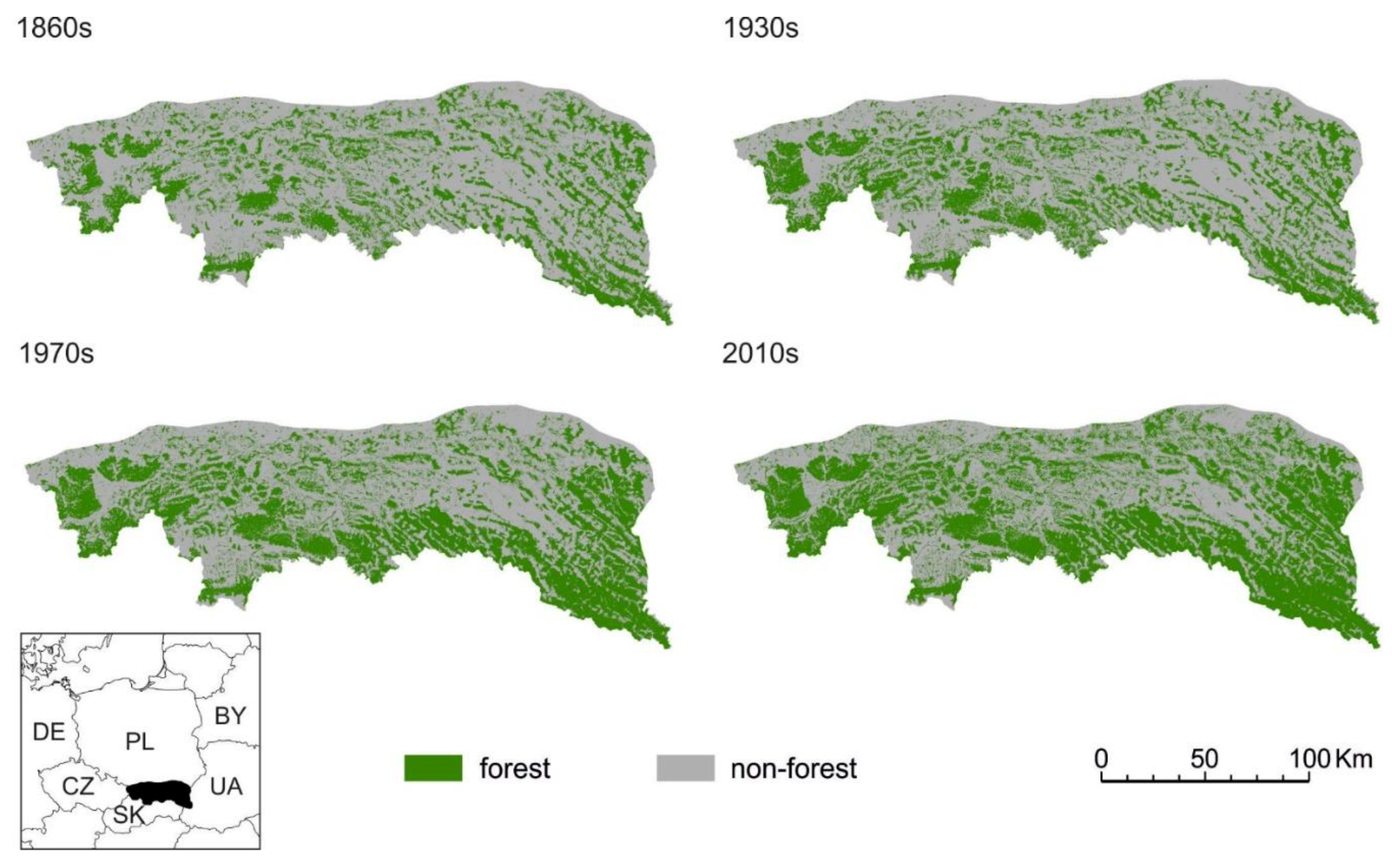
2.1. Study Area and Forest Data

The Polish Carpathians are located in the northern part of the Carpathian arc with altitudes ranging from 300 masl at the northern margin of the Carpathian foothills, and 2500 masl in the Polish part of the Tatra Mountains [43]. Forest transition started in the region in the mid-19th century when forest cover amounted to 27% [44,45]. As in all Carpathian countries, land-use change was driven by frequent regime shifts related to the complex history of the region [46]. Currently, typical landscapes in the Polish Carpathians consist of a mosaic of agricultural lands and forests, with most settlements located in valleys, and forests cover 47% of the area [45]. In the 1840s, almost all forests belonged to properties of large landowners [47]. After World War II, forest properties larger than 25 ha were nationalized and, currently, approximately 50% of forests in the Carpathians are owned by the State Forests National Holding. According to [33], approximately 14% of the farmland shows signs of secondary forest succession, and therefore forest-cover increase in the region is expected in the near future [48].
The pattern change of forest fragmentation and its relationship to forest area were analyzed in four time steps: the 1860s, 1930s, 1970s and 2010s (Figure 1). The boundaries of the forested areas in the 1860s and 1930s forest maps were obtained using manual vectorization of topographic maps, the Austro-Hungarian Second Military Survey Map (1:28,800; quick looks available at http://mapire.eu/), and the Polish Military Map (1:100,000; maps can be consulted at http://hgis.cartomatic.pl/), respectively. For the 1970s we extracted forest-cover information using a semi-automated feature-extraction procedure based on color separation and morphological processing followed by manual correction [49] applied to the Polish Topographic Map (1:25,000; available at http://mapy.geoportal.gov.pl/), published by the Head Office of Geodesy and Cartography (Główny Urząd Geodezji i Kartografii, GUGIK). The 2010s forest map was obtained through the integration of different available land-use and land-cover spatial databases. A primary data source on forest boundaries was the contemporary Polish national topographic vector database in scale 1:10,000 (BDOT10k, available at http://mapy.geoportal.gov.pl/), further verified using data from the Forest Numerical Map, the Forest Data Bank (https://www.bdl.lasy.gov.pl/portal/), the Polish Topographic Map for 1970s (1:25,000) and aerial and satellite imagery acquired between 2009 and 2015 (available at http://mapy.geoportal.gov.pl/). Forest maps for all time steps were converted to raster format with 10 m spatial resolution.

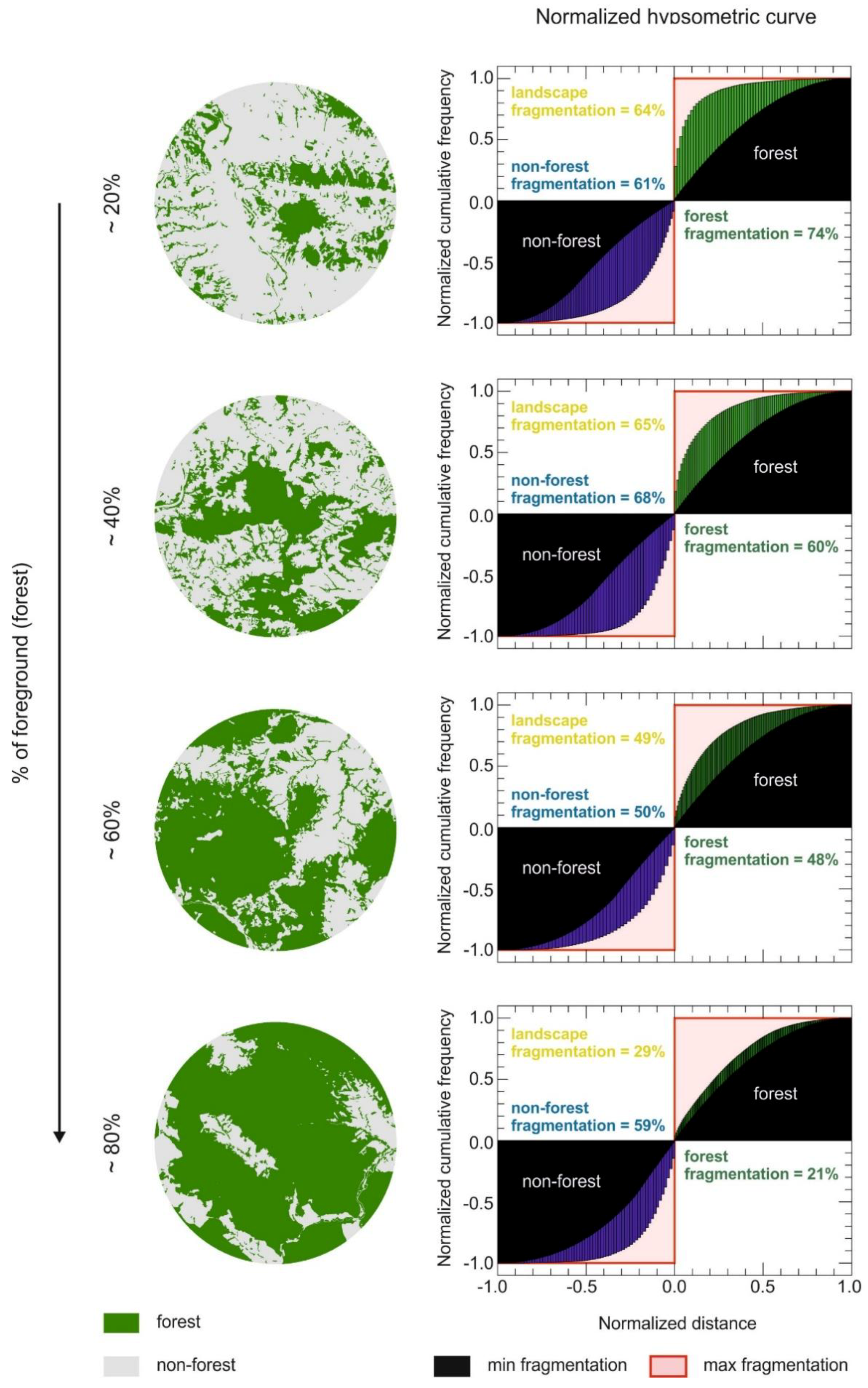
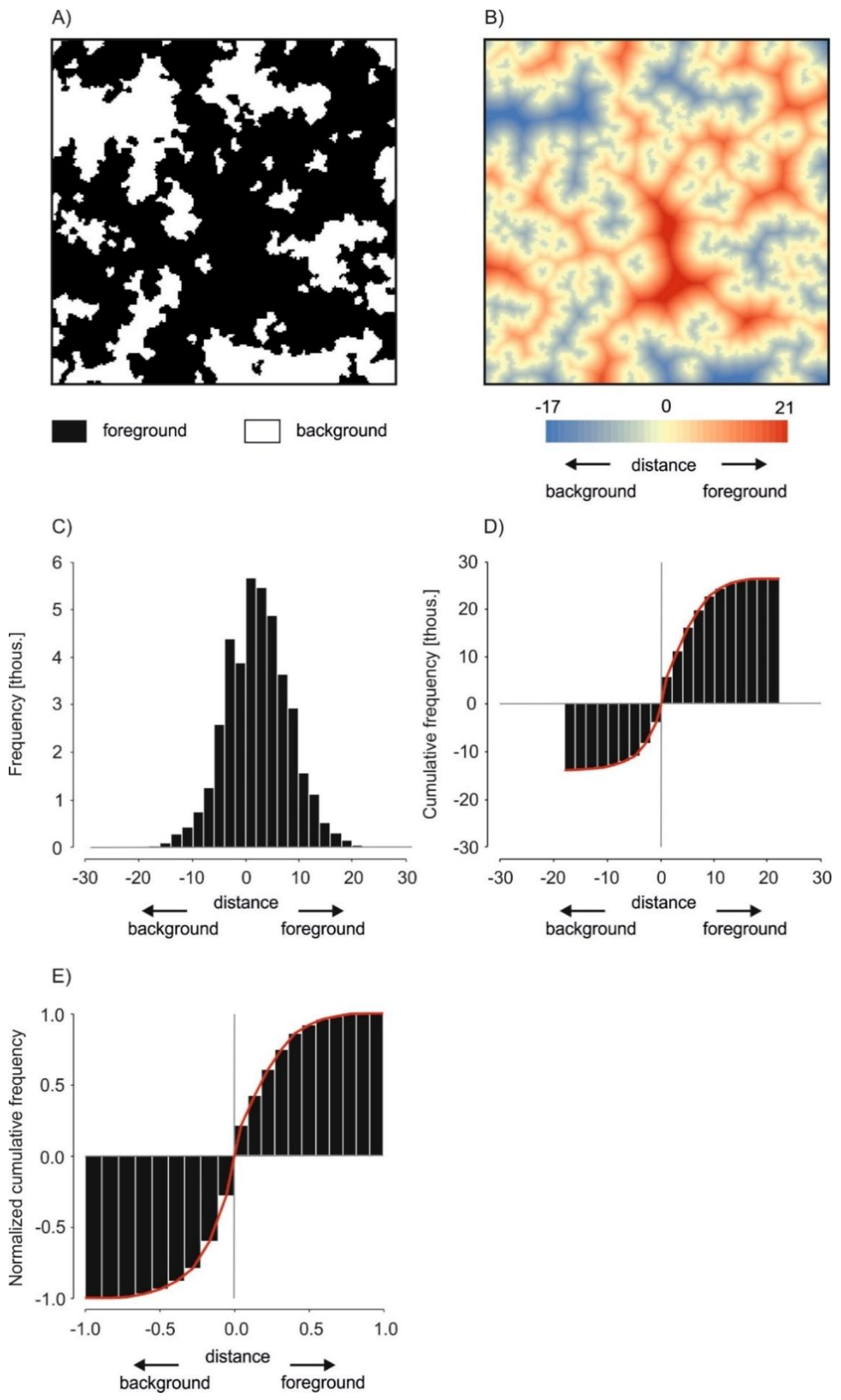
2.2. Landscape Hypsometric Curve and Forest-Fragmentation Index

Forest fragmentation was quantified with the software GuidosToolbox, version 2.6 [50] using measures based on the LHC (see Appendix A for a detailed description). Principally, those measures are based on distances to forest edges which are mostly used in landscape fragmentation studies to assess forest, or landscape dissection by roads (roadless volume) [9,51,52,53]. As implemented in GuidosToolbox, LHC summarizes the Euclidean distance distribution for a given binary landscape map, in which the foreground class represents the land-cover class of interest (here forest), and the background class represents the complementary class (here non-forest). Euclidean distances are calculated as positive values in the foreground and negative values in the background land-cover class. LHC is further normalized, i.e., scaled by the theoretical maximum distance in the foreground and in the background. The degree of fragmentation corresponds to the area under the LHC covered between minimum possible fragmentation (for a landscape with the same foreground area but clumped in a single circle) and maximum fragmentation (for a chessboard-like landscape configuration of foreground patches and foreground coverage of 50%). Fragmentation is then calculated separately for the foreground and background class, as well as summarized for the whole landscape (Appendix A, Equations (A1)–(A3)).
The LHC approach allows for a simultaneous account of different fragmentation aspects, including perforations, amount, division and dispersion of habitat patches, and provides one single value ranging from 0% to 100% referring to fragmentation, in this sense being an overall fragmentation measure. Based on the LHC concept, we defined the forest-fragmentation index as the degree of fragmentation of foreground area for a forest/non-forest binary map.

2.3. Quantifying Forest Fragmentation and Its Changes

We analyzed forest-fragmentation and forest-cover changes based on LHC in 127 randomly selected circular test areas with 5-km radii (an area of approximately 80 km2, close to the area of a typical commune in the study area) and with minimum distance between centers of circles equal to 5 km (that, is partial overlap was allowed). To ensure an even coverage of the entire study area, the Polish Carpathians were covered by the regular grid of 20 × 20 km square units, and at least one circle center-point was located in each unit. For each circular test area and time step, we calculated the LHC-based forest-fragmentation index (as described above), as well as forest-cover area. For each of the time periods (1860s–1930s, 1930s–1970s and 1970s–2010s), the change rates of forest fragmentation and the change rates of forest cover were calculated as a relative difference between the end- and the initial values.
Finally, for each test area we assessed its forest-fragmentation trajectory (FFT). An FFT was one of 27 possible sequences of stable, increasing or decreasing forest fragmentation in three analyzed time periods (for instance, a test area could have decreasing forest fragmentation in the period 1860s–1930s, a stable forest fragmentation in the period 1930s–1970s, and an increasing forest fragmentation in the period 1970s–2010s). Fragmentation for a given period was labelled as stable if the fragmentation change rate was lower than ¼ of the standard deviation of change rates for all analyzed test areas: below 1.45% for the period 1860s–1930s, below 1.81% for the period 1930s–1970s, and below 1.18% for the period 1970s–2010s.

2.4. Quantifying Potential Determinants of Forest Fragmentation

For each circular test area we calculated the percentage of forest structural components. To assess forest structure, we used morphological image segmentation available in GuidosToolbox [50]. Following [54], each forest pixel was categorized as either core forest (no non-forest neighbors), edge forest (at the outside of larger forest patches), loop/bridge/branch forest (thin, elongated forest structures with no core forest, attached to large forest patches), perforated forest (edges along openings inside larger forest patches), and islet forests (patches too small to contain core forest), using the forest edge width of 30 m (3 pixels). Change rates of forest structural components for each time period were then calculated in the same way as for forest fragmentation and forest cover, i.e., as a relative difference between the end- and the initial values.

3. Results

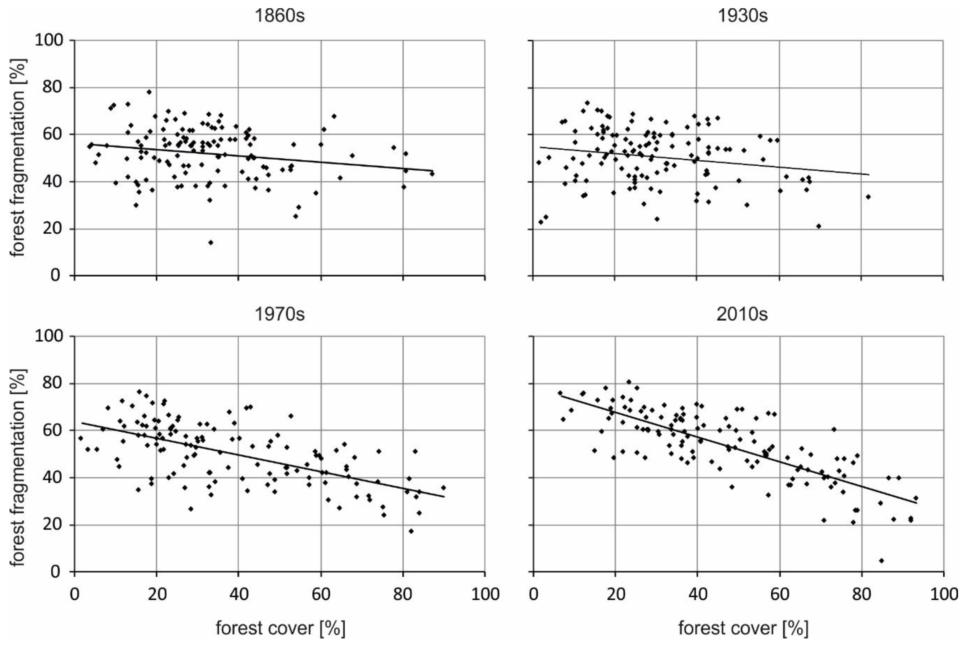
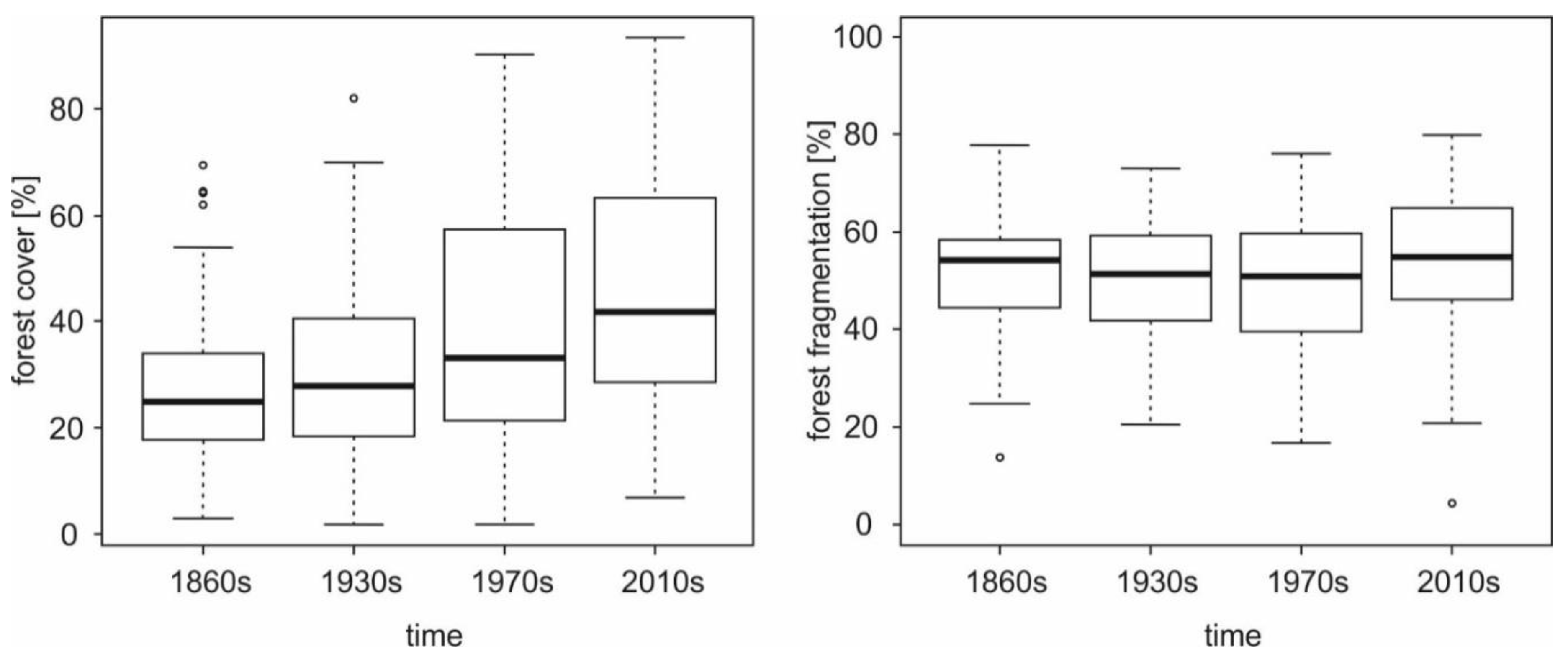
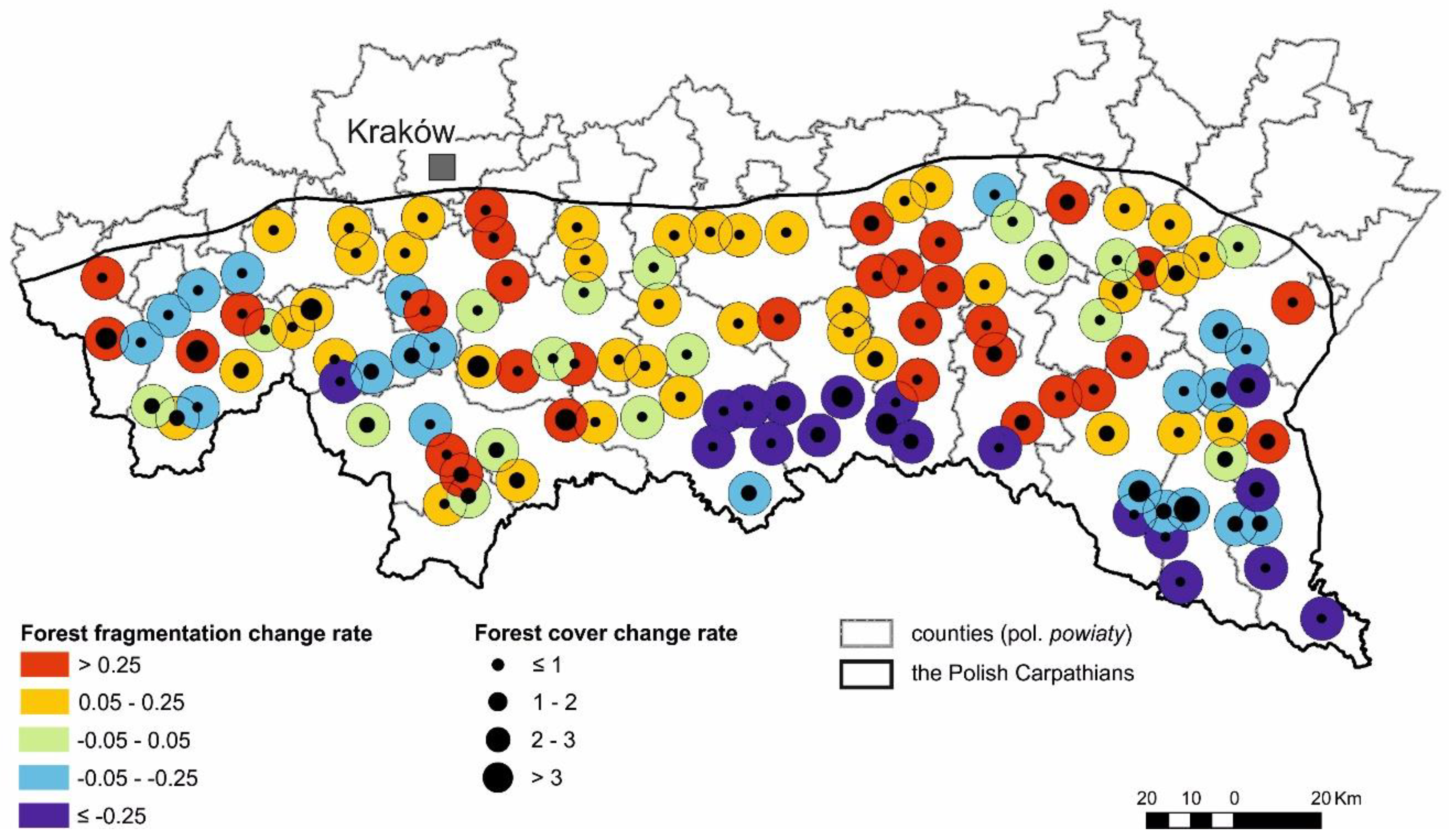
3.1. Patterns of Forest Fragmentation and Its Relation to Forest Area

Average forest fragmentation in the Polish Carpathians remained stable between the 1860s and 2010s, at an approximate level of 55% (Figure 2). However, we found fluctuations in specific periods: a general decrease of forest fragmentation between the 1860s and 1930s (in 57% of test areas), and a general increase between the 1930s and 1970s and between the 1970s and 2010s (in 58% and 72% of test areas, respectively). This trajectory of forest fragmentation was observed in the context of a significant increase of forest area in the region over the entire study period, from 27% to 47% (Figure 2). Most of the test areas experienced forest-cover increase through the whole analyzed period (61%). Forest-cover decrease was found in 34% of the test areas between the 1860s and 1930s, and in only 7% of the test areas between the 1930s and 1970s. Between the 1970s and 2010s, forest cover was increasing in all test areas.
We found no clear pattern when analyzing forest fragmentation in relation to forest area for the 1860s and 1930s (Figure 3). A negative relation between forest-fragmentation and forest-cover areas was found for the 1970s and 2010s, where forest area explained 38% and 61% of variation in forest fragmentation, respectively (Figure 3).
Changes in forest fragmentation differed also regionally. Looking at the entire study period, 1860s–2010s, forest fragmentation decreased most significantly in the south and south-eastern part of the region (Bieszczady and Beskid Niski Mountains), corresponding with the highest forest increase rates, while forest fragmentation increased mostly in the northern and central part of the study area. Several areas with high forest-cover increase rates showed decreases of fragmentation, yet in some cases we observed high forest-cover increase rates alongside fragmentation increase (Figure 4). In general, we found no clear correlation between forest-fragmentation change rate and forest-cover change rate for all analyzed time periods as well as for the whole studied period (R2 ≤ 0.1), with the sign of the relation variable in time: neutral for the period 1860s–1930s (and overall, 1860s–2010s), weakly negative for the period 1930s–1970s, and weakly positive for the period 1970s–2010s (Figure 5).

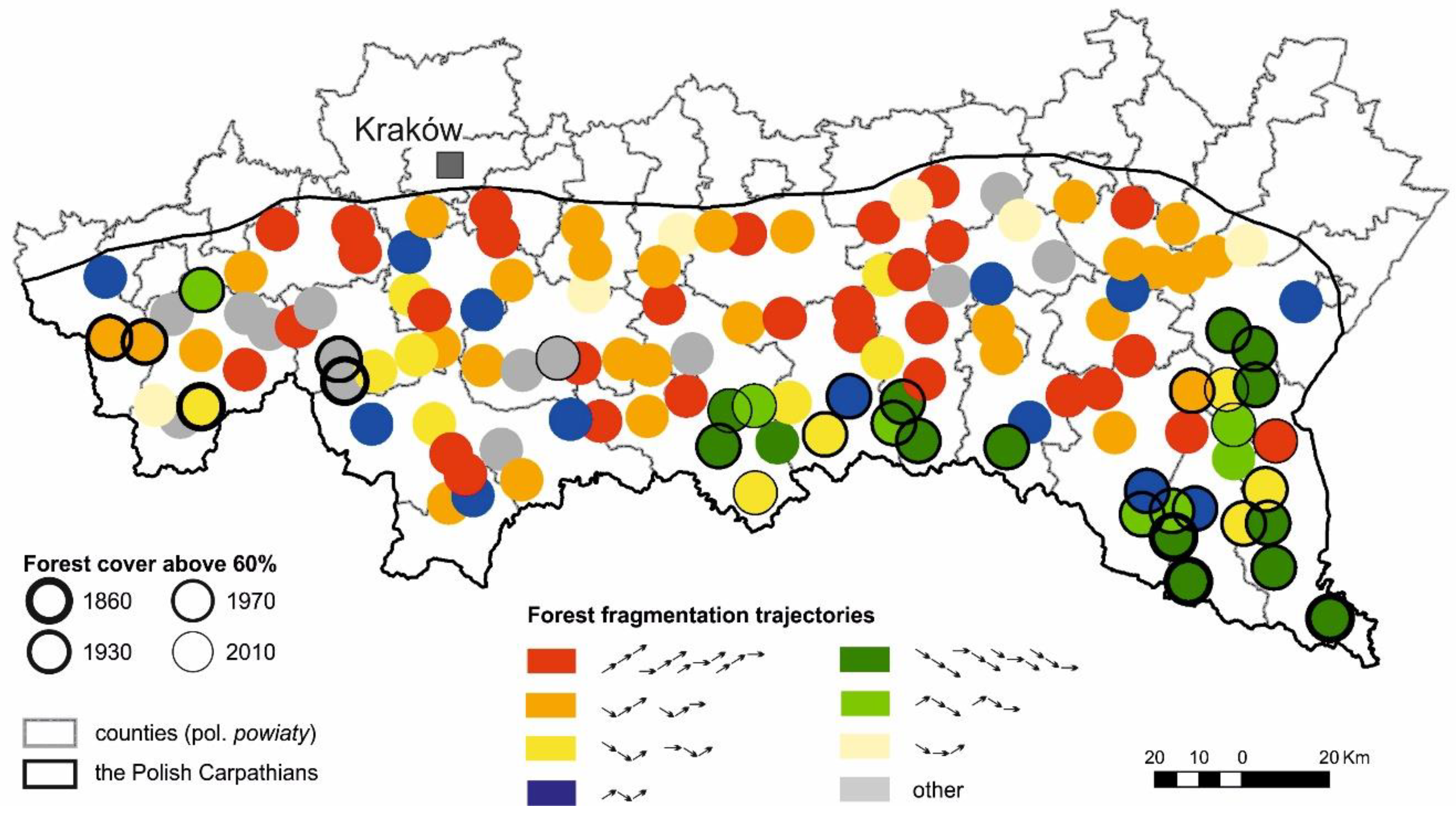
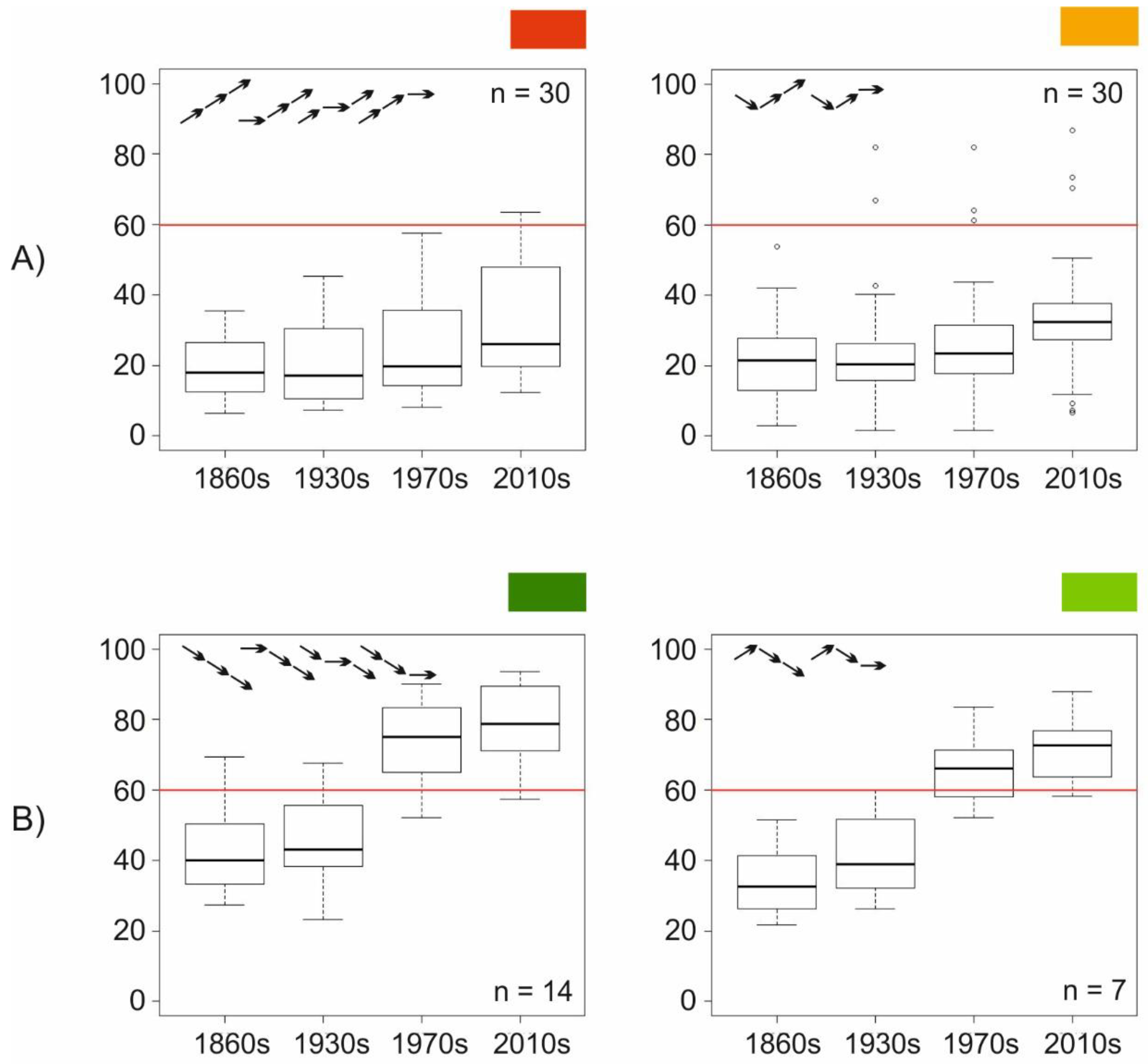
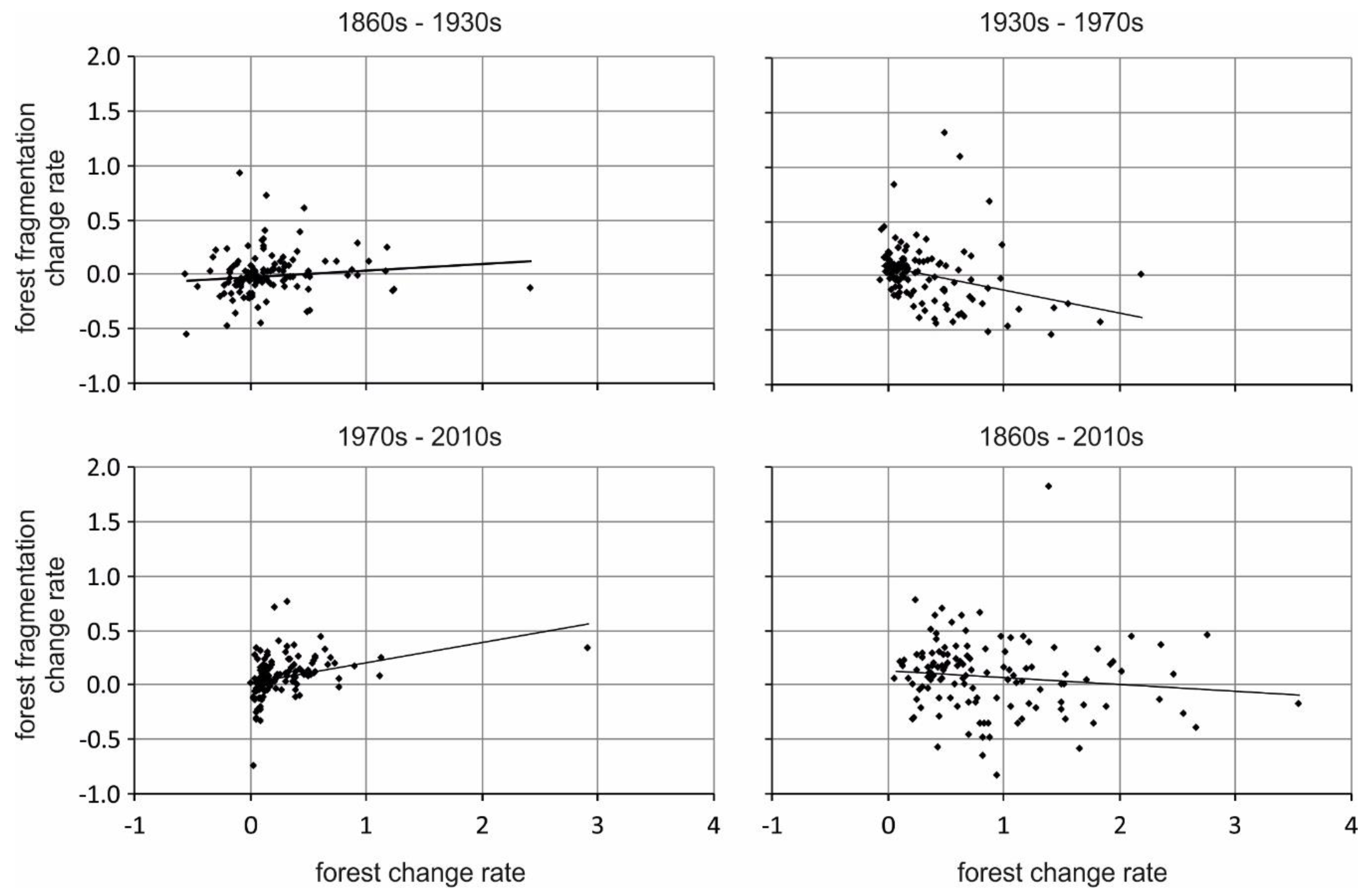
3.2. Forest-Fragmentation Trends

In our study area we found 22 individual FFTs (out of 27 theoretically possible ones). We found important regional differences in the distribution of trajectories in the study area (Figure 6): decreasing fragmentation was found mostly in the south-eastern part of the Polish Carpathians, while increasing fragmentation was prevalent in the northern part of the study area. The two most common trends were: decrease in forest fragmentation between the 1860s and 1930s and then increase in forest fragmentation between the 1930s and 2010s (24% of test areas), and increase in forest fragmentation throughout the whole analyzed period (24% of test areas). Test areas with these trajectories were characterized by the lowest forest-cover area in all time steps (Figure 7A). Decrease of forest fragmentation between the 1860s and 2010s and increase in forest fragmentation in the first period (1860s–1930s) followed by decrease in forest fragmentation in the second and third periods (1930s–1970s and 1970s–2010s) were found in 11% and 6% of test areas, respectively. Test areas with these trajectories were characterized by the highest forest-cover area in all time steps, with mean forest-cover percentage exceeding 60% already in the 1970s (Figure 7B).

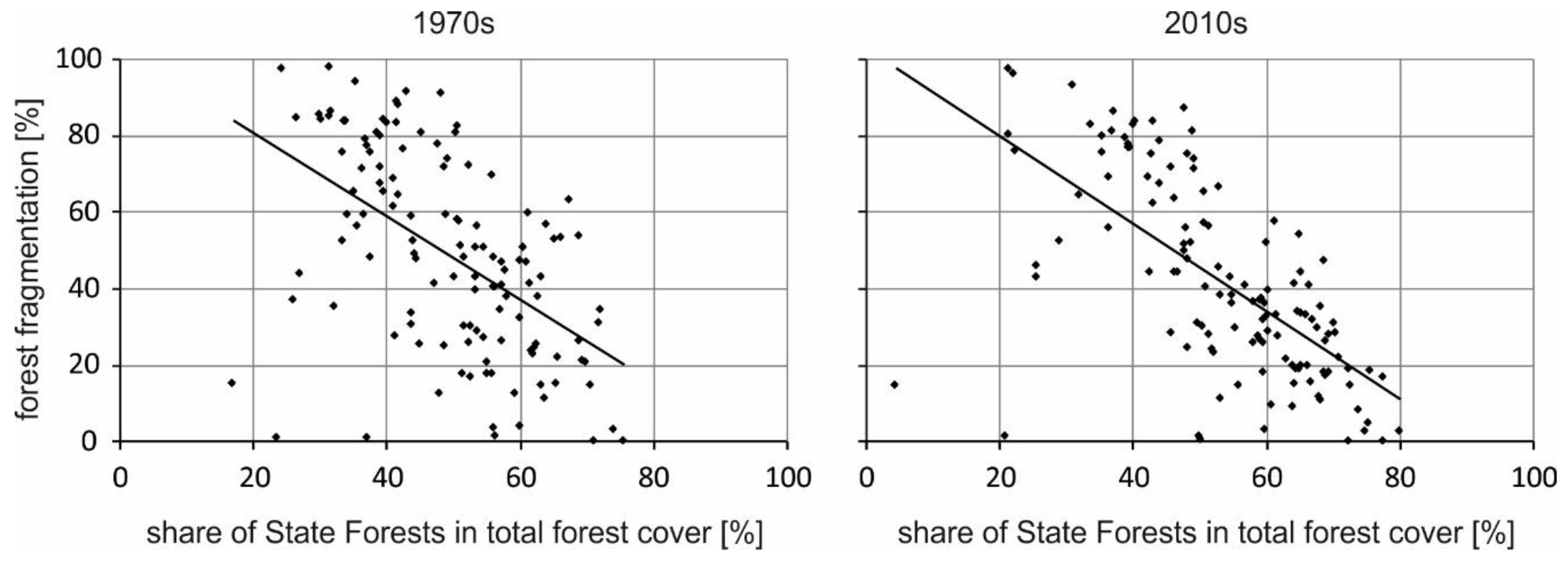
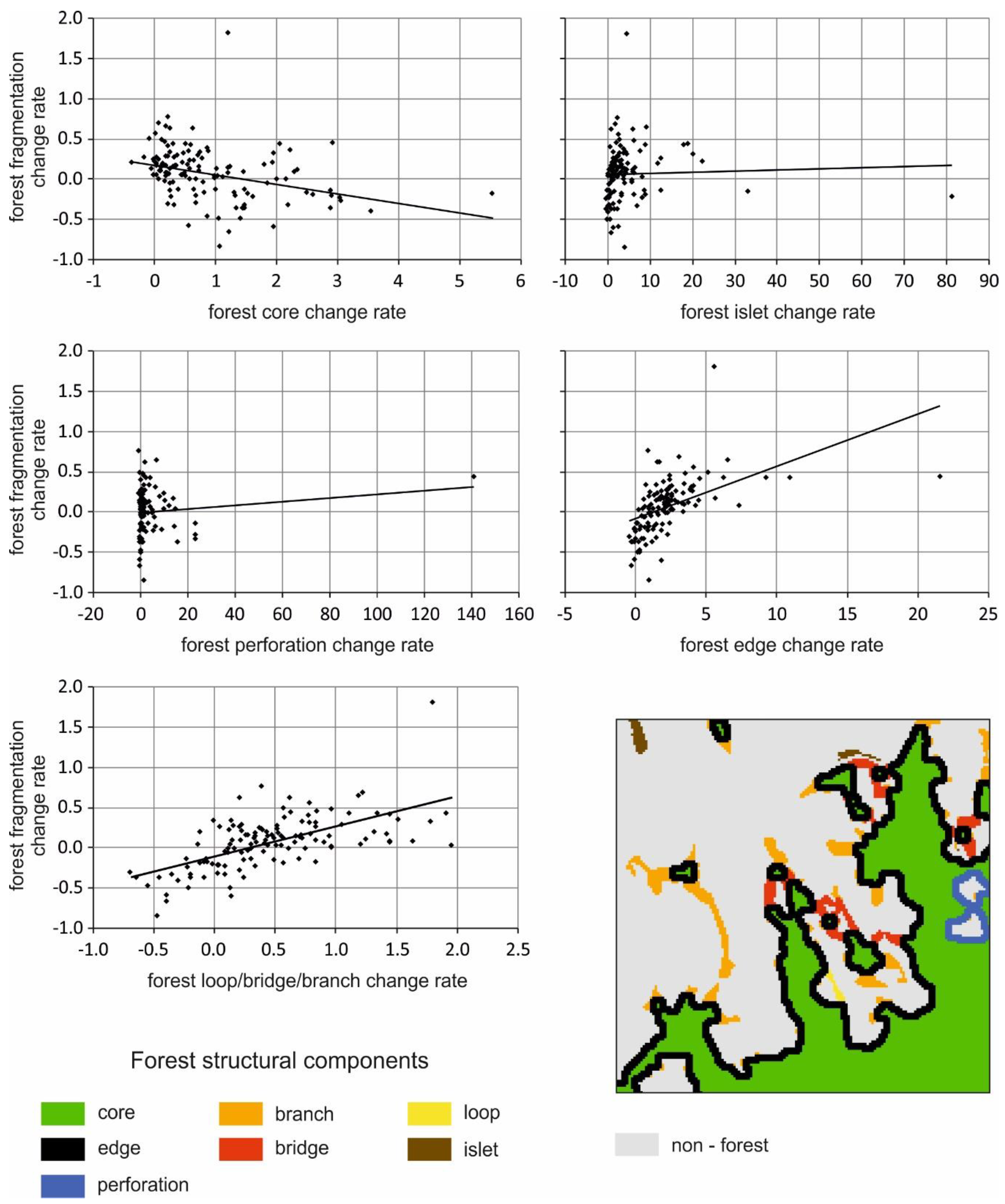
3.3. Dynamics of Forest Fragmentation and Structural Components

For the entire studied period (1860s–2010s), forest fragmentation change rates were negatively related to forest core change rate, and positively related to forest edge and forest loop/bridge/branch change rates (Figure 8). We found no significant relation of forest fragmentation to the changing amount of forest islets and perforations (R2 ≤ 0.01).

4. Discussion

We mapped forest cover for four time steps (1860s, 1930s, 1970s, 2010s) for the entire Polish Carpathians, and analyzed forest fragmentation using the LHC method. Forest fragmentation was then related to changes in forest cover and the amount of forest structural components. Our study thus spans 150 years, providing insights into long-term forest fragmentation trends over a large area. Only a few studies provide a comparable temporal framework [23,55], as many studies on forest increase and fragmentation change use remotely sensed data covering relatively short periods of 10–20 years. Due to the length of the studied period, and a relatively gradual change in forest cover over more than 150 years, to assess and compare forest fragmentation in space and time we used the LHC method, offering a uniform morphometric concept to measure the actual degree of fragmentation in a generic way.
Although not explicitly tested in this study, it is expected that LHC is sensitive to spatial data generalization, similar to many other fragmentation measures [56,57]. This may, in particular, apply to the map set of the 1930s with the scale 1:100,000, the only available for the study area for the interwar period, and the Austro-Hungarian Second Military Survey Map, the oldest map data used in our study. Our previous tests related to the consistency of the historical maps of the Polish Carpathians in the context of land-cover change analysis [58] showed, however, that spatial detail for the map set of the 1930s with the scale 1:100,000 is comparable with maps in much higher scale. Similarly, the Austro-Hungarian Second Military Survey Map was generalized from the 1:2880 cadastral maps and retains a very high level of detail in presenting land cover [59]. It was also successfully used in other land-use and land-cover change studies in the region [60]. We conclude, therefore, that the set of maps used to analyze long-term forest fragmentation changes has sufficient consistency in spite of various spatial scales’ generalization levels, yet the results need to be interpreted with caution.
Contrary to the expectations—that increasing forest cover causes decreasing forest fragmentation—we received several results showing lack of straightforward relation between forest cover and forest fragmentation. First, in spite of a significant forest-cover increase in the entire study area, forest fragmentation was found to be stable. Next, for the first (1860s) and second (1930s) time steps, the correlation between forest cover and forest fragmentation was found to be insignificant. Finally, we observed no significant correlation between forest-cover change rates and forest-fragmentation change rates for all analyzed periods (1860s–1930s, 1930s–1970s, 1970s–2010s, 1860s–2010s). These results, however, do not signify a lack of relationship between forest area and forest fragmentation, but rather imply its complexity. In the northern and north-western part of the study area, characterized mainly by low forest cover and slow forest increase, we found forest-cover increase related to increasing forest fragmentation. In such landscapes with initially low forest cover adding more forest is likely to happen in the form of isolated patches or irregular branches, thus triggering an increase in fragmentation. On the other hand, in the south-eastern part of the study area, where resettlements after World War II triggered land abandonment and quick forest expansion [40,61], we observed decreasing fragmentation (Figure 7). When forest cover is high, adding more forest is likely to happen through the merging of already existing forest patches or the closure of perforations inside forests, both resulting in a decrease of fragmentation. In our case, decreasing fragmentation in the study area was clearly visible when forest cover exceeded 60%, and this observation is in line with various studies which have shown the relation between the amount of cover and the pattern structures and the significant change of this relation close to the percolation threshold of 59.3% [62,63,64]. Importantly, random landscape analysis with LHC-based fragmentation index showed a similar effect already above 50% of foreground (Appendix A), although this slightly lower threshold is less evident in the real-world data. The transition of forest cover over the percolation threshold occurred in many test areas only in the last two time steps (1970s and 2010s). This is why the insignificant correlation between forest cover and forest fragmentation was noted in the 1860s and 1930s (most test areas had forest cover with values below 60% and high fragmentation levels) and why it turned to a significant negative correlation in the 1970s and 2010s (test areas had either high fragmentation levels for forest cover below 60% or low fragmentation with forest cover above 60%, Figure 3). Our results show that the habitat (e.g., forests) fragmentation does not need to be closely correlated with the amount of habitat (for instance, [65]), thus offering space to test empirically habitat amount–species richness relationships in landscapes with variable fragmentation of habitats as suggested by [25].
The increase of forest fragmentation in areas with increasing forest cover reflects the fact that forest-cover increase in the Polish Carpathians has occurred mostly through land abandonment and secondary forest succession on private farmland, composed of a huge number of very small parcels making up farms of individual landowners [33]. In this way, several new structural elements appear in the landscape, contributing to changes of fragmentation. Our results indicate that while loops, bridges, branches and edges were positively correlated with and contributed to increased forest fragmentation, islets and perforations had no significant influence. We hypothesize that although forest perforations—for instance, former pastures—are likely to disappear from the mountain landscapes [66,67] thus decreasing forest fragmentation, this change is not counterbalancing the effect of an emerging mosaic of forested and open land on overall forest fragmentation. The mosaic develops on the formerly homogenous farmland following decisions of individual landowners to abandon particular land parcels that later undergo secondary forest succession. As land abandonment occurs more frequently close to existing forests [33], new forested parcels are likely to form various branch-type patterns, thus increasing forest fragmentation. That land ownership has an effect on forest fragmentation is further confirmed by the significant negative correlation between the proportion of large forest estates managed by the State Forests National Holding and forest fragmentation (Figure 9).
Several studies point to the importance of land-use legacies and persistence for current dynamics of the landscape [39]. For instance, contemporary land abandonment in the Carpathian countries depends on the former land use, and length of cultivation period [38]. Our results prove the importance of land-ownership boundaries established in the past for contemporary forest expansion patterns and fragmentation of forest habitats. Up to the World War II period, farmland area, though split into a huge number of land parcels, was relatively homogenous and intensively used [67], forming the landscape matrix for forest patches being parts of large land properties [47]. In the post-war period, decline of agriculture triggered decisions by individual farmers leading to gradual conversion of several land parcels into forests, contributing to the current, highly fragmented landscape mosaic and increase of forest fragmentation in most of the study area except where forest cover significantly exceeded the percolation threshold.

5. Conclusions

Our study shows that increasing forest cover may trigger increasing or decreasing forest fragmentation, depending on the rate, extent and causes of forest-cover increase. In the first case, mostly in the north and western part of the Polish Carpathians, a typical, gradual forest expansion is framed by well-established land ownership boundaries and individual decisions of land owners which lead to the conversion of small farmland plots to forest patches in a mosaic-type fashion. How this “bottom-up” forest expansion transforms the Carpathian landscape differs significantly from changes imposed by political decisions and affecting large areas. Such a “top-down” large-scale forest expansion occurred between the 1930s and 1970s in the south-eastern part of the Polish Carpathians, following forced depopulation and extensive land abandonment by entire communes. These changes, independent of the individual decisions of land owners, resulted in the formation of extensive, homogenous forest patches, contributing to decreasing forest fragmentation. We conclude, therefore, that understanding the causes of the forest-cover increase is important to disentangle how it further contributes to changes of forest fragmentation. Knowledge of land abandonment and forest expansion trends and their causes may, thus, support landscape planning, for instance in the context of green infrastructures [68] designed to maintain landscape biodiversity and the connectivity of habitats. Appropriately targeted policies may trigger farmland to forest conversion in areas forming important corridors for wildlife, and prevent the conversion where it may negatively impact biodiversity.

Author Contributions

J.K. conceived the study and wrote the manuscript. E.Z. conceived the study, designed the experiment, performed the calculations, prepared the figures and wrote the manuscript. P.V. designed the landscape hypsometric curve tool and wrote the manuscript. M.D., D.K., N.K. and K.O. prepared the forest maps, commented and edited the manuscript.

Acknowledgments

Forest-cover maps were developed within the FORECOM project (Forest-cover changes in mountainous regions—drivers, trajectories and implications, PSRP 008/2010), supported by a grant from Switzerland through the Swiss contribution to the enlarged European Union.

Conflicts of Interest

The authors declare no conflict of interest. The founding sponsors had no role in the design of the study; in the collection, analyses, or interpretation of data; in the writing of the manuscript; and in the decision to publish the results.

Appendix A. Description of a New Fragmentation Index Based on a Landscape Hypsometric Curve

A hypsometric curve represents a cumulative distribution function of elevations in a given area. However, the concept can be extended to the so-called landscape hypsometric curve (LHC), which summarizes the distance distribution for a given binary landscape map in which the foreground depicts the class of interest, and the background depicts the complementary class. Examples of landscape binary masks include a forest/non-forest mask, a wetland/non-wetland mask, or a grassland/non-grassland mask. However, foreground/background classes can be also defined based on a multi-criteria approach to distinguish, for instance, habitat/non-habitat areas for a given species.
In the first step, for a given binary landscape map (Figure A1A), distances from foreground/background edge are calculated as positive values within a foreground class and negative values outside a foreground class (i.e., within a background class; Figure A1B). Typically, Euclidean distances are applied; however, functional distances can also be calculated within a landscape to construct LHC. The frequency distribution of distances (Figure A1C) depends on the amount of foreground/background classes in the landscape, and their configuration. In the next step, cumulated frequency distributions of distances are calculated, separately for the foreground and background, and a continuous function, i.e., LHC, is fitted to the resulting plot (Figure A1D). LHC is further normalized, i.e., scaled by the maximum distance in the foreground and in the background (Figure A1E).
The shape of the normalized LHC summarizes a spatial structure of a given landscape: the closer to Y axes the normalized LHC is, the bigger is the fragmentation of the foreground/background class (Figure A2). Therefore, for a given landscape, the degree of fragmentation corresponds to the area under the LHC covered between minimum possible fragmentation (black, Figure A2) and maximum fragmentation (red, Figure A2). By minimum possible fragmentation, we understand fragmentation of a landscape with the same proportion of foreground but maximum foreground aggregation, i.e., all foreground pixels are accumulated to a circle in the center of the landscape. By maximum fragmentation we understand fragmentation of a checkerboard-type landscape, with 50% foreground coverage. This theoretical maximum condition for fragmentation is characterized by all foreground as well as all background pixels having a distance of 1 and thus a cumulative distance represented by the step-function outlined in red in Figure A2.
The area under the LHC is calculated separately for the foreground (frag_FG, area highlighted in green in Figure A2) and background (frag_BG, area highlighted in blue in Figure A2) class. Foreground and background fragmentation is defined then as, respectively:
f r a g _ F G = 0 1 N L H C F G 0 1 N L H C F G M N ,
f r a g _ B G = 1 0 N L H C B G 1 0 N L H C B G M N ,
where NLHCFG/NLHCBG is a normalized LHC for the foreground/background class of a given landscape, and NLHCFGMIN/NLHCBGMIN is a normalized LHC for the foreground/background class of a landscape with the same proportion of foreground but maximum foreground aggregation (i.e., minimum fragmentation).
Figure A1. Summary of landscape hypsometric curve (LHC) concept: (A) an exemplary binary landscape map; (B) a distance map for foreground and background classes of the binary map; (C) frequency distribution of distance values; (D) cumulative frequency distribution of distance values with LHC marked in red; (E) normalized cumulative frequency distribution of distance values with normalized LHC marked in red.
Sustainability 10 01472 g0a1
Figure A2. Normalized LHCs and fragmentation indices calculated for exemplary test areas with different forest cover. The landscape fragmentation index is shown in yellow, while fragmentation of its foreground (i.e., forest) component in green, and of its background component (i.e., non-forest) in blue.
Sustainability 10 01472 g0a2
Accounting for the dual nature of fragmentation (foreground is fragmented by background and vice versa), the degree of fragmentation for a given landscape is defined by the weighted sum of fragmentation in the foreground and the background:
frag = (AFG/100 × frag_FG) + (ABG/100 × frag_BG),
where AFG/ABG is the foreground/background area, respectively, and frag_FG/frag_BG is the foreground/background fragmentation, respectively.
The landscape fragmentation index as designed provides values in the range of 0–100%, accounting for and summarizing key fragmentation aspects: duality, perforations, amount, division, and dispersion of image objects. To illustrate the behavior of the LHC-based fragmentation index, we computed it for a series of simulated binary (foreground/background) landscapes with known landscape patterns using tools implemented in the GuidosToolbox software [50]. To generate artificial landscapes, we applied the modified random cluster algorithm [69], implemented as ‘randomHabitat’ function within the ‘secr’ R library [70].
The ‘RandomHabitat’ function generates patches according to the initial probability (parameter p), which controls the degree of aggregation or fragmentation of the simulated landscape. Then, patches composed of marked pixels are identified based on a certain neighborhood rule (parameter directions = rook’s move 4 or queen’s move 8) and assigned to either habitat (foreground) class or non-habitat (background) class based on the class abundance probability (parameter A = expected proportion of habitat). Both random and clumped landscape maps can be generated. For smaller p values, more fragmented landscapes with a large number of small patches will be generated, while larger p values generate more aggregated landscapes with more large patches. Specifically, a simple random map is obtained when p is close to 0.
Artificial landscapes were generated by varying three landscape pattern attributes:
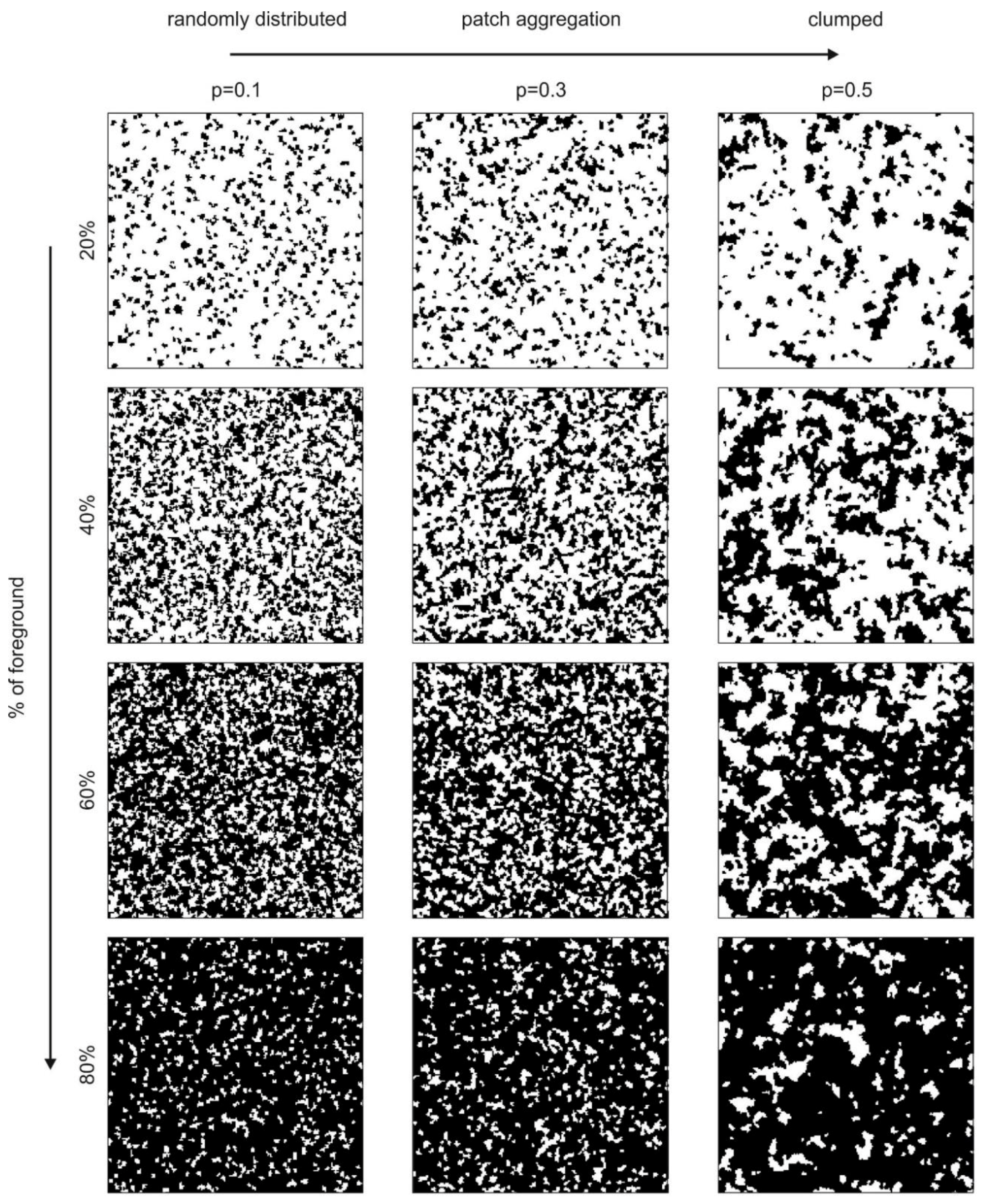
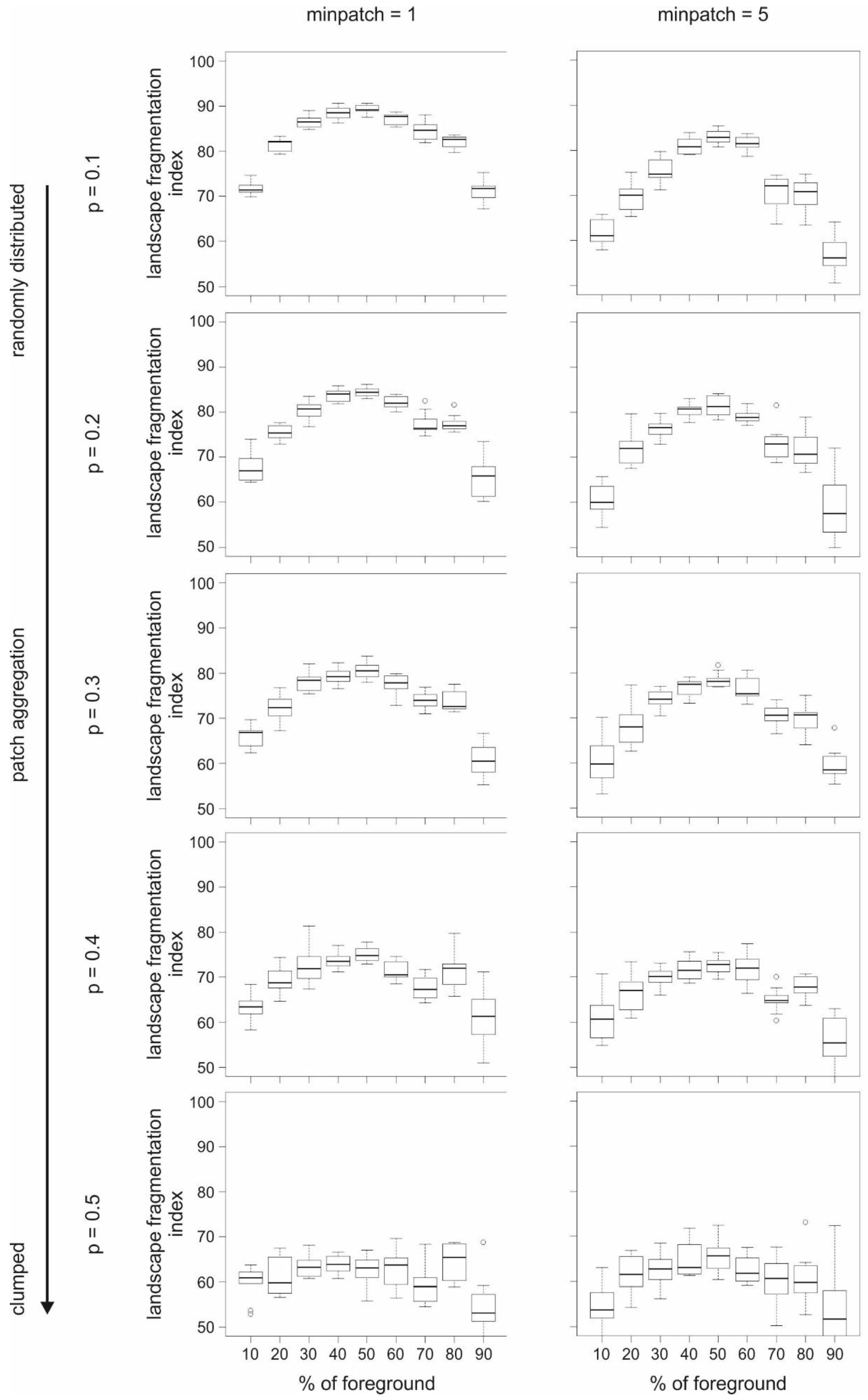
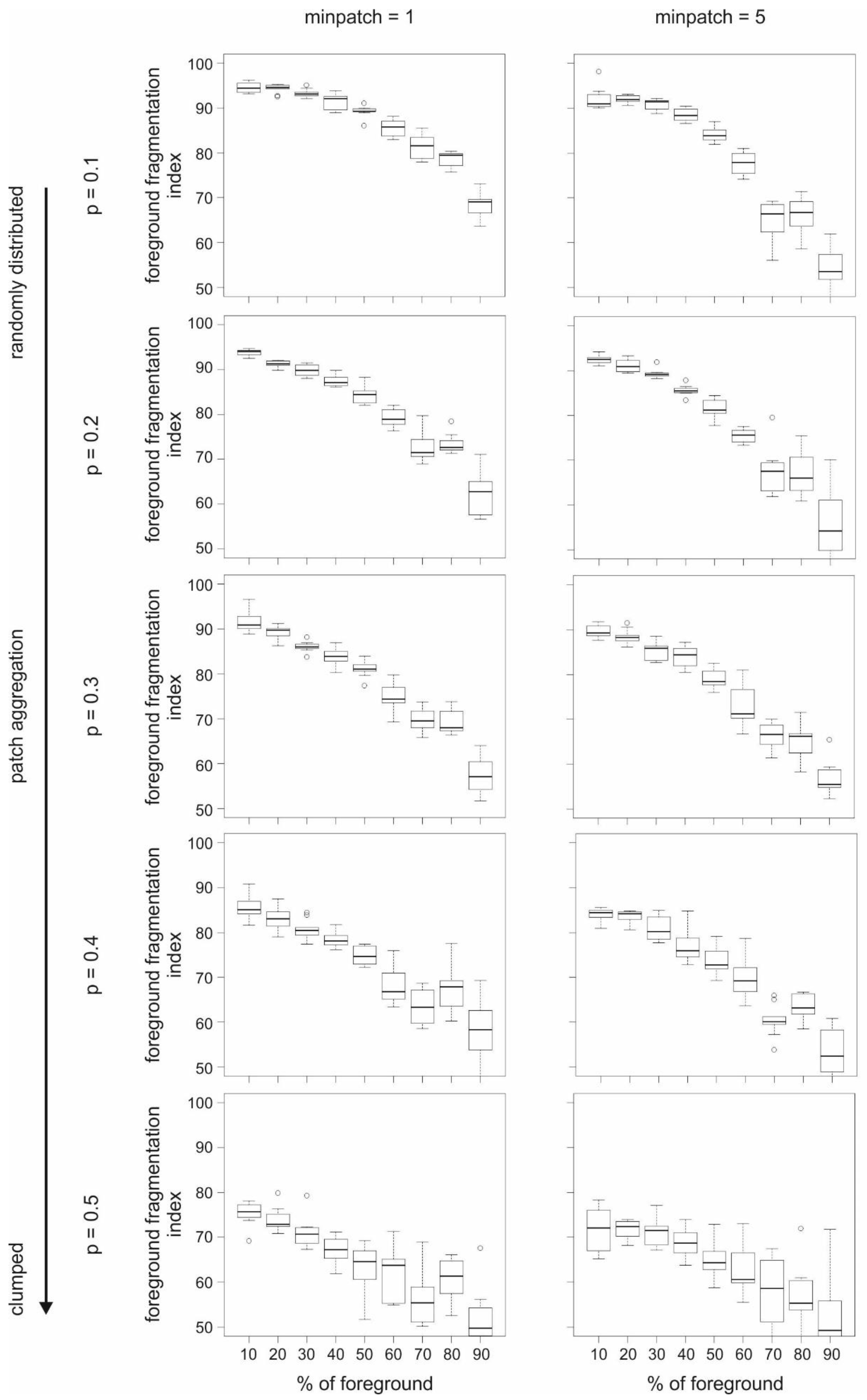
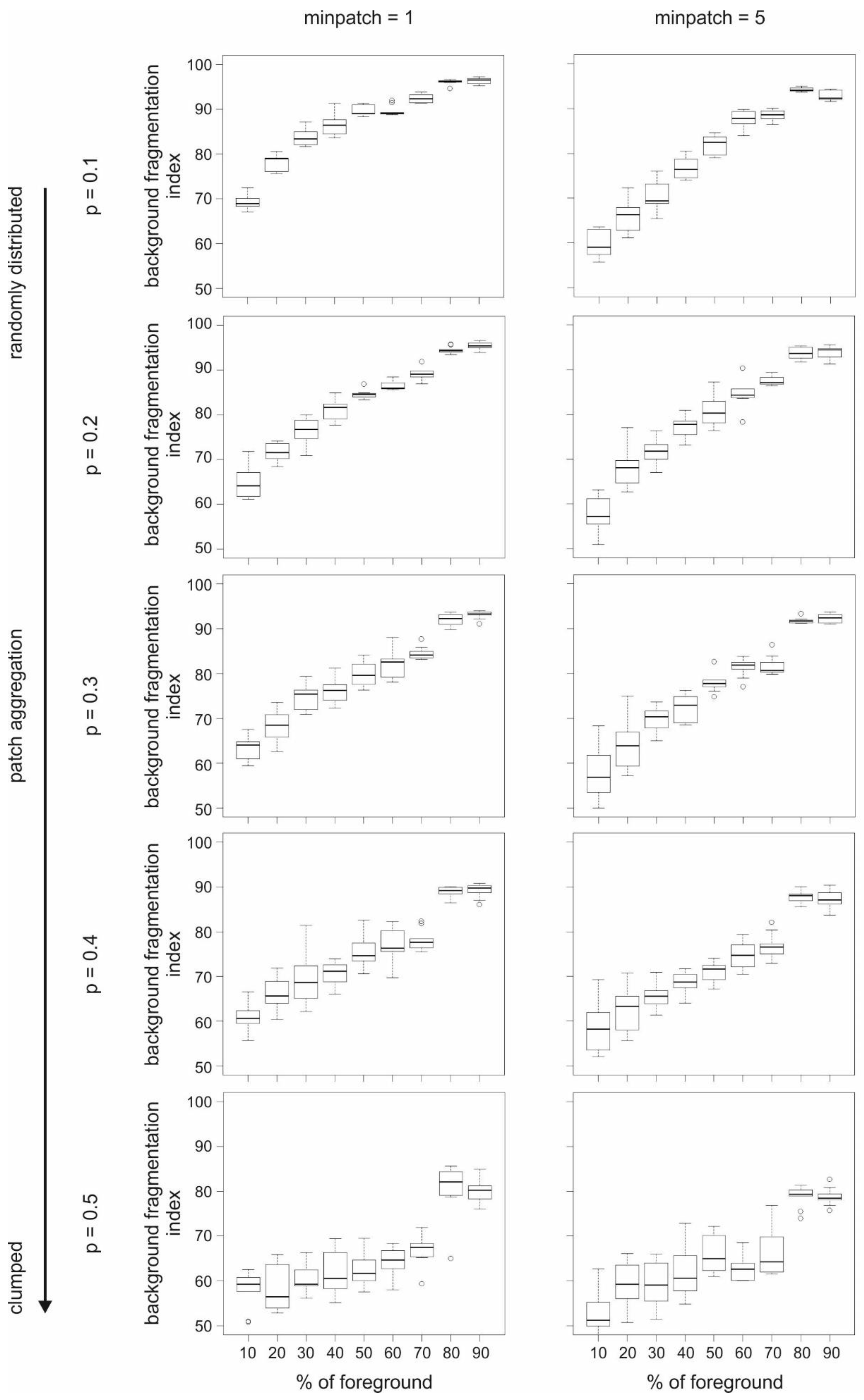
  • Class abundance distribution (A) being the proportion of the whole landscape area occupied by the foreground class; with 9 values ranging from 10% to 90%, with a 10% step;
  • Patch aggregation/clumpiness (p), i.e., spatial distribution patterns of patches; with 5 values ranging from 0.1 (randomly distributed) to 0.5 (clumped), with a step of 0.1;
  • Minimum patch size (minpatch) with 2 values: 1 or 5.
In this way, we received in total 90 combinations (Figure A3). For each combination, we generated 10 replicate landscapes. In all simulated landscapes, rook’s move was used as a neighborhood rule.
Generally, the highest degree of landscape fragmentation measured by the LHC-based landscape fragmentation index was found for simulated landscapes with around 50% of foreground coverage (Figure A4). For foreground coverage below 50%, there was a positively correlated relationship between foreground coverage and the LHC-based landscape fragmentation index. For foreground coverage exceeding 50%, we found a negatively correlated relationship between foreground coverage and the LHC-based landscape fragmentation index (Figure A4, Table A1). These findings are in line with expectations: when foreground cover is low (<50%) adding foreground cover into an empty landscape will form more patches, thus increasing fragmentation. When foreground cover is more than 50%, further adding foreground cover will close up existing holes and increase the extent of compact foreground area, hence fragmentation will decrease. However, for simulated landscapes with minpatch = 1 and the highest degree of aggregation (p = 0.5), this relationship was slightly weaker (R2 = 0.62 for foreground coverage ≤50%; and R2 = 0.31 for foreground coverage ≥50%, Table A1). In terms of foreground and background fragmentation components, foreground fragmentation decreased (Figure A5; R2 ≥ 0.89, Table A1) and background fragmentation increased (Figure A6; R2 ≥ 0.80, Table A1) with increasing foreground coverage, respectively. As with the LHC-based landscape fragmentation index, its foreground and background components decreased with increasing patch aggregation from p = 0.1 to p = 0.5 (Figure A4, Figure A5 and Figure A6).
Figure A3. Examples of simulated landscapes with varying percentage of foreground and patch aggregation (minpatch = 5) used for testing properties of the LHC-based fragmentation index.
Sustainability 10 01472 g0a3
Figure A4. Boxplots illustrating the effects of landscape pattern attributes on values of the LHC-based landscape fragmentation index.
Sustainability 10 01472 g0a4
Table A1. Coefficients of determination and signs of relation between the LHC-based fragmentation index (and its foreground and background components) and the foreground coverage for simulated landscapes with varying pattern attributes.
minpatch = 1
pfragfrag_FGfrag_BG
0.1(a) (+) 0.85(−) 0.89(+) 0.90
(b) (−) 0.86
0.2(a) (+) 0.91(−) 0.94(+) 0.97
(b) (−) 0.84
0.3(a) (+) 0.88(−) 0.96(+) 0.98
(b) (−) 0.83
0.4(a) (+) 0.88(−) 0.94(+) 0.95
(b) (−) 0.67
0.5(a) (+) 0.62(−) 0.93(+) 0.80
(b) (−) 0.31
minpatch = 5
0.1(+) 0.97(−) 0.90(+) 0.96
(−) 0.91
0.2(+) 0.87(−) 0.95(+) 0.97
(−) 0.89
0.3(+) 0.92(−) 0.96(+) 0.98
(−) 0.91
0.4(+) 0.89(−) 0.94(+) 0.96
(−) 0.76
0.5(+) 0.83(−) 0.93(+) 0.86
(−) 0.82
(a) Foreground coverage ≤50%; (b) foreground coverage ≥50%.
Figure A5. Boxplots illustrating the effects of landscape pattern attributes on values of the LHC-based foreground fragmentation index.
Sustainability 10 01472 g0a5
Figure A6. Boxplots illustrating the effects of landscape pattern attributes on values of the LHC-based background fragmentation index.
Sustainability 10 01472 g0a6

References

  1. Fardila, D.; Kelly, L.T.; Moore, J.L.; McCarthy, M.A. A systematic review reveals changes in where and how we have studied habitat loss and fragmentation over 20 years. Biol. Conserv. 2017, 212, 130–138. [Google Scholar] [CrossRef]
  2. Fischer, J.; Lindenmayer, D.B. Landscape modification and habitat fragmentation: A synthesis. Glob. Ecol. Biogeogr. 2007, 16, 265–280. [Google Scholar] [CrossRef]
  3. Haddad, N.M.; Brudvig, L.A.; Clobert, J.; Davies, K.F.; Gonzalez, A.; Holt, R.D.; Lovejoy, T.E.; Sexton, J.O.; Austin, M.P.; Collins, C.D.; et al. Habitat fragmentation and its lasting impact on Earth’s ecosystems. Sci. Adv. 2015, 1, e1500052. [Google Scholar] [CrossRef] [PubMed]
  4. Pfeifer, M.; Lefebvre, V.; Peres, C.A.; Banks-Leite, C.; Wearn, O.R.; Marsh, C.J.; Butchart, S.H.M.; Arroyo-Rodríguez, V.; Barlow, J.; Cerezo, A.; et al. Creation of forest edges has a global impact on forest vertebrates. Nature 2017, 551, 187–191. [Google Scholar] [CrossRef] [PubMed]
  5. Abdullah, S.A.; Nakagoshi, N. Forest fragmentation and its correlation to human land use change in the state of Selangor, peninsular Malaysia. For. Ecol. Manag. 2007, 241, 39–48. [Google Scholar] [CrossRef]
  6. Harper, G.J.; Steininger, M.K.; Tucker, C.J.; Juhn, D.; Hawkins, F. Fifty years of deforestation and forest fragmentation in Madagascar. Environ. Conserv. 2007, 34, 325–333. [Google Scholar] [CrossRef]
  7. Li, M.; Zhu, Z.; Vogelmann, J.E.; Xu, D.; Wen, W.; Liu, A. Characterizing fragmentation of the collective forests in southern China from multitemporal Landsat imagery: A case study from Kecheng district of Zhejiang province. Appl. Geogr. 2011, 31, 1026–1035. [Google Scholar] [CrossRef]
  8. Reddy, C.S.; Sreelekshmi, S.; Jha, C.S.; Dadhwal, V.K. National assessment of forest fragmentation in India: Landscape indices as measures of the effects of fragmentation and forest cover change. Ecol. Eng. 2013, 60, 453–464. [Google Scholar] [CrossRef]
  9. Ahmed, S.E.; Lees, A.C.; Moura, N.G.; Gardner, T.A.; Barlow, J.; Ferreira, J.; Ewers, R.M. Road networks predict human influence on Amazonian bird communities. Proc. R. Soc. B Biol. Sci. 2014, 281. [Google Scholar] [CrossRef] [PubMed]
  10. Molinario, G.; Hansen, M.C.; Potapov, P.V. Forest cover dynamics of shifting cultivation in the Democratic Republic of Congo: A remote sensing-based assessment for 2000–2010. Environ. Res. Lett. 2015, 10. [Google Scholar] [CrossRef]
  11. Tapia-Armijos, M.F.; Homeier, J.; Espinosa, C.I.; Leuschner, C.; de la Cruz, M. Deforestation and Forest Fragmentation in South Ecuador since the 1970s—Losing a Hotspot of Biodiversity. PLoS ONE 2015, 10, e0133701. [Google Scholar] [CrossRef] [PubMed]
  12. Liu, Y.; Feng, Y.; Zhao, Z.; Zhang, Q.; Su, S. Socioeconomic drivers of forest loss and fragmentation: A comparison between different land use planning schemes and policy implications. Land Use Policy 2016, 54, 58–68. [Google Scholar] [CrossRef]
  13. Sharma, M.; Areendran, G.; Raj, K.; Sharma, A.; Joshi, P.K. Multitemporal analysis of forest fragmentation in Hindu Kush Himalaya—A case study from Khangchendzonga Biosphere Reserve, Sikkim, India. Environ. Monit. Assess. 2016, 188. [Google Scholar] [CrossRef] [PubMed]
  14. Chakraborty, A.; Ghosh, A.; Sachdeva, K.; Joshi, P.K. Characterizing fragmentation trends of the Himalayan forests in the Kumaon region of Uttarakhand, India. Ecol. Inform. 2017, 38, 95–109. [Google Scholar] [CrossRef]
  15. Reddy, C.S.; Vazeed Pasha, S.; Satish, K.V.; Saranya, K.R.L.; Jha, C.S.; Krishna Murthy, Y.V.N. Quantifying nationwide land cover and historical changes in forests of Nepal (1930–2014): Implications on forest fragmentation. Biodivers. Conserv. 2017, 27, 91–107. [Google Scholar] [CrossRef]
  16. Rosa, I.M.D.; Gabriel, C.; Carreiras, J.M.B. Spatial and temporal dimensions of landscape fragmentation across the Brazilian Amazon. Reg. Environ. Chang. 2017, 17, 1687–1699. [Google Scholar] [CrossRef] [PubMed]
  17. Sharma, M.; Chakraborty, A.; Garg, J.K.; Joshi, P.K. Assessing forest fragmentation in north-western Himalaya: A case study from Ranikhet forest range, Uttarakhand, India. J. For. Res. 2017, 28, 319–327. [Google Scholar] [CrossRef]
  18. Ramachandran, R.M.; Roy, P.S.; Chakravarthi, V.; Sanjay, J.; Joshi, P.K. Long-term land use and land cover changes (1920–2015) in Eastern Ghats, India: Pattern of dynamics and challenges in plant species conservation. Ecol. Indic. 2018, 85, 21–36. [Google Scholar] [CrossRef]
  19. Kozak, J.; Estreguil, C.; Vogt, P. Forest cover and pattern changes in the Carpathians over the last decades. Eur. J. For. Res. 2007, 126, 77–90. [Google Scholar] [CrossRef]
  20. Zhou, W.; Huang, G.; Pickett, S.T.A.; Cadenasso, M.L. 90 Years of Forest Cover Change in an Urbanizing Watershed: Spatial and Temporal Dynamics. Landsc. Ecol. 2011, 26, 645–659. [Google Scholar] [CrossRef]
  21. Gong, C.; Yu, S.; Joesting, H.; Chen, J. Determining socioeconomic drivers of urban forest fragmentation with historical remote sensing images. Landsc. Urban Plan. 2013, 117, 57–65. [Google Scholar] [CrossRef]
  22. Gao, Q.; Yu, M. Discerning fragmentation dynamics of tropical forest and wetland during reforestation, Urban Sprawl, and policy shifts. PLoS ONE 2014, 9, e0113140. [Google Scholar] [CrossRef] [PubMed]
  23. Camarretta, N.; Puletti, N.; Chiavetta, U.; Corona, P. Quantitative changes of forest landscapes over the last century across Italy. Plant Biosyst. Int. J. Deal. All Asp. Plant Biol. 2017, 1–9. [Google Scholar] [CrossRef]
  24. Xie, H.; He, Y.; Zhang, N.; Lu, H. Spatiotemporal changes and fragmentation of forest land in Jiangxi Province, China. J. For. Econ. 2017, 29, 4–13. [Google Scholar] [CrossRef]
  25. Fahrig, L. Rethinking patch size and isolation effects: The habitat amount hypothesis. J. Biogeogr. 2013, 40, 1649–1663. [Google Scholar] [CrossRef]
  26. Meyfroidt, P.; Lambin, E.F. Global Forest Transition: Prospects for an End to Deforestation. Annu. Rev. Environ. Resour. 2011, 36, 343–371. [Google Scholar] [CrossRef]
  27. Mather, A.S. The forest transition. Area 1992, 24, 367–379. [Google Scholar]
  28. Grainger, A. The forest transition: An alternative approach. Area 1995, 27, 242–251. [Google Scholar]
  29. Rudel, T.K.; Coomes, O.T.; Moran, E.; Achard, F.; Angelsen, A.; Xu, J.; Lambin, E. Forest transitions: Towards a global understanding of land use change. Glob. Environ. Chang. 2005, 15, 23–31. [Google Scholar] [CrossRef]
  30. MacDonald, D.; Crabtree, J.R.; Wiesinger, G.; Dax, T.; Stamou, N.; Fleury, P.; Gutierrez Lazpita, J.; Gibon, A. Agricultural abandonment in mountain areas of Europe: Environmental consequences and policy response. J. Environ. Manag. 2000, 59, 47–69. [Google Scholar] [CrossRef]
  31. Price, B.; Kienast, F.; Seidl, I.; Ginzler, C.; Verburg, P.H.; Bolliger, J. Future landscapes of Switzerland: Risk areas for urbanisation and land abandonment. Appl. Geogr. 2015, 57, 32–41. [Google Scholar] [CrossRef]
  32. Pazúr, R.; Lieskovský, J.; Feranec, J.; Oťaheľ, J. Spatial determinants of abandonment of large-scale arable lands and managed grasslands in Slovakia during the periods of post-socialist transition and European Union accession. Appl. Geogr. 2014, 54, 118–128. [Google Scholar] [CrossRef]
  33. Kolecka, N.; Kozak, J.; Kaim, D.; Dobosz, M.; Ostafin, K.; Ostapowicz, K.; Wężyk, P.; Price, B. Understanding farmland abandonment in the Polish Carpathians. Appl. Geogr. 2017, 88, 62–72. [Google Scholar] [CrossRef]
  34. Baumann, M.; Kuemmerle, T.; Elbakidze, M.; Ozdogan, M.; Radeloff, V.C.; Keuler, N.S.; Prishchepov, A.V.; Kruhlov, I.; Hostert, P. Patterns and drivers of post-socialist farmland abandonment in Western Ukraine. Land Use Policy 2011, 28, 552–562. [Google Scholar] [CrossRef]
  35. Campagnaro, T.; Frate, L.; Carranza, M.L.; Sitzia, T. Multi-scale analysis of alpine landscapes with different intensities of abandonment reveals similar spatial pattern changes: Implications for habitat conservation. Ecol. Indic. 2017, 74, 147–159. [Google Scholar] [CrossRef]
  36. Terres, J.-M.; Scacchiafichi, L.N.; Wania, A.; Ambar, M.; Anguiano, E.; Buckwell, A.; Coppola, A.; Gocht, A.; Källström, H.N.; Pointereau, P.; et al. Farmland abandonment in Europe: Identification of drivers and indicators, and development of a composite indicator of risk. Land Use Policy 2015, 49, 20–34. [Google Scholar] [CrossRef]
  37. Munteanu, C.; Kuemmerle, T.; Keuler, N.S.; Müller, D.; Balázs, P.; Dobosz, M.; Griffiths, P.; Halada, L.; Kaim, D.; Király, G.; et al. Legacies of 19th century land use shape contemporary forest cover. Glob. Environ. Chang. 2015, 34, 83–94. [Google Scholar] [CrossRef]
  38. Munteanu, C.; Kuemmerle, T.; Boltiziar, M.; Lieskovský, J.; Mojses, M.; Kaim, D.; Konkoly-Gyuró, É.; Mackovčin, P.; Müller, D.; Ostapowicz, K.; et al. Nineteenth-century land-use legacies affect contemporary land abandonment in the Carpathians. Reg. Environ. Chang. 2017, 17, 2209–2222. [Google Scholar] [CrossRef]
  39. Lieskovský, J.; Bürgi, M. Persistence in cultural landscapes: A pan-European analysis. Reg. Environ. Chang. 2017, 18, 175–187. [Google Scholar] [CrossRef]
  40. Kozak, J.; Estreguil, C.; Troll, M. Forest cover changes in the northern Carpathians in the 20th century: A slow transition. J. Land Use Sci. 2007, 2, 127–146. [Google Scholar] [CrossRef]
  41. Bolliger, J.; Schmatz, D.; Pazúr, R.; Ostapowicz, K.; Psomas, A. Reconstructing forest-cover change in the Swiss Alps between 1880 and 2010 using ensemble modelling. Reg. Environ. Chang. 2017, 17, 2265–2277. [Google Scholar] [CrossRef]
  42. Loran, C.; Munteanu, C.; Verburg, P.H.; Schmatz, D.R.; Bürgi, M.; Zimmermann, N.E. Long-term change in drivers of forest cover expansion: An analysis for Switzerland (1850–2000). Reg. Environ. Chang. 2017, 17, 2223–2235. [Google Scholar] [CrossRef]
  43. Balon, J.; German, K.; Kozak, J.; Malara, H.; Widacki, W.; Ziaja, W. Regiony fizycznogeograficzne. In Karpaty Polskie; Warszyńska, J., Ed.; Uniwersytet Jagielloński: Kraków, Poland, 1995; pp. 117–130. ISBN 83-233-0852-7. [Google Scholar]
  44. Kozak, J. Forest Cover Changes and Their Drivers in the Polish Carpathian Mountains since 1800. In Reforesting Landscapes Linking Pattern and Process; Nagendra, H., Southworth, J., Eds.; Springer: Dordrecht, The Netherlands; Heidelberg, Germany; London, UK; New York, NY, USA, 2010; pp. 253–273. ISBN 978-1-4020-9655-6. [Google Scholar]
  45. Kozak, J.; Szwagrzyk, M. Have there been forest transitions? Forest transition theory revisited in the context of the Modifiable Areal Unit Problem. Area 2016, 48, 504–512. [Google Scholar] [CrossRef]
  46. Munteanu, C.; Radeloff, V.; Griffiths, P.; Halada, L.; Kaim, D.; Knorn, J.; Kozak, J.; Kuemmerle, T.; Lieskovsky, J.; Müller, D.; et al. Land change in the Carpathian region before and after major institutional changes. In Land-Cover and Land-Use Changes in Eastern Europe after the Collapse of the Soviet Union in 1991; Gutman, G., Radeloff, V., Eds.; Springer: Cham, Switzerland, 2017; pp. 57–90. ISBN 978-3-319-42636-5. [Google Scholar]
  47. Ślusarek, K. Rola gospodarcza lasów w dobrach ziemskich w Galicji w XIX w. Stud. Mater. Ośr. Kult. Leśne. 2014, 13, 357–374. [Google Scholar]
  48. Price, B.; Kaim, D.; Szwagrzyk, M.; Ostapowicz, K.; Kolecka, N.; Schmatz, D.R.; Wypych, A.; Kozak, J. Legacies, socio-economic and biophysical processes and drivers: The case of future forest cover expansion in the Polish Carpathians and Swiss Alps. Reg. Environ. Chang. 2017, 17, 2279–2291. [Google Scholar] [CrossRef]
  49. Ostafin, K.; Iwanowski, M.; Kozak, J.; Cacko, A.; Gimmi, U.; Kaim, D.; Psomas, A.; Ginzler, C.; Ostapowicz, K. Forest cover mask from historical topographic maps based on image processing. Geosci. Data J. 2017, 4, 29–39. [Google Scholar] [CrossRef]
  50. Vogt, P.; Riitters, K. GuidosToolbox: Universal digital image object analysis. Eur. J. Remote Sens. 2017, 50, 352–361. [Google Scholar] [CrossRef]
  51. Watts, R.D.; Compton, R.W.; McCammon, J.H.; Rich, C.L.; Wright, S.M.; Owen, T.; Ouren, D.S. Roadless space of the conterminous United States. Science 2007, 316, 736–738. [Google Scholar] [CrossRef] [PubMed]
  52. Nega, T.; Smith, C.; Bethune, J.; Fu, W.H. An analysis of landscape penetration by road infrastructure and traffic noise. Comput. Environ. Urban Syst. 2012, 36, 245–256. [Google Scholar] [CrossRef]
  53. Ibisch, P.L.; Hoffmann, M.T.; Kreft, S.; Pe’Er, G.; Kati, V.; Biber-Freudenberger, L.; DellaSala, D.A.; Vale, M.M.; Hobson, P.R.; Selva, N. A global map of roadless areas and their conservation status. Science 2016, 354, 1423–1427. [Google Scholar] [CrossRef] [PubMed]
  54. Soille, P.; Vogt, P. Morphological segmentation of binary patterns. Pattern Recognit. Lett. 2009, 30, 456–459. [Google Scholar] [CrossRef]
  55. Zhou, W.; Zhang, S.; Yu, W.; Wang, J.; Wang, W. Effects of Urban Expansion on Forest Loss and Fragmentation in Six Megaregions, China. Remote Sens. 2017, 9, 991. [Google Scholar] [CrossRef]
  56. Saura, S. Effects of remote sensor spatial resolution and data aggregation on selected fragmentation indices. Landsc. Ecol. 2004, 19, 197–209. [Google Scholar] [CrossRef]
  57. Townsend, P.A.; Lookingbill, T.R.; Kingdon, C.C.; Gardner, R.H. Spatial pattern analysis for monitoring protected areas. Remote Sens. Environ. 2009, 113, 1410–1420. [Google Scholar] [CrossRef]
  58. Kaim, D.; Kozak, J.; Ostafin, K.; Dobosz, M.; Ostapowicz, K.; Kolecka, N.; Gimmi, U. Uncertainty in historical land-use reconstructions with topographic maps. Quaest. Geogr. 2014, 33, 55–63. [Google Scholar] [CrossRef]
  59. Kaim, D.; Kozak, J.; Kolecka, N.; Ziółkowska, E.; Ostafin, K.; Ostapowicz, K.; Gimmi, U.; Munteanu, C.; Radeloff, V.C. Broad scale forest cover reconstruction from historical topographic maps. Appl. Geogr. 2016, 67, 39–48. [Google Scholar] [CrossRef]
  60. Feurdean, A.; Munteanu, C.; Kuemmerle, T.; Nielsen, A.B.; Hutchinson, S.M.; Ruprecht, E.; Parr, C.L.; Perşoiu, A.; Hickler, T. Long-term land-cover/use change in a traditional farming landscape in Romania inferred from pollen data, historical maps and satellite images. Reg. Environ. Chang. 2017, 17, 2193–2207. [Google Scholar] [CrossRef]
  61. Affek, A. Spatially explicit changes in land ownership through 3 socio-political systems: A case study from southeast Poland. Geogr. Pol. 2015, 88, 519–530. [Google Scholar] [CrossRef]
  62. Gardner, R.H.; Milne, B.T.; Turner, M.G.; O’Neill, R.V. Neutral models for the analysis of broad-scale landscape pattern. Landsc. Ecol. 1987, 1, 19–28. [Google Scholar] [CrossRef]
  63. De Oliveira Filho, F.J.B.; Metzger, J.P. Thresholds in landscape structure for three common deforestation patterns in the Brazilian Amazon. Landsc. Ecol. 2006, 21, 1061–1073. [Google Scholar] [CrossRef]
  64. Riitters, K.H.; Vogt, P.; Soille, P.; Kozak, J.; Estreguil, C. Neutral model analysis of landscape patterns from mathematical morphology. Landsc. Ecol. 2007, 22, 1033–1043. [Google Scholar] [CrossRef]
  65. Hanski, I. Habitat fragmentation and species richness. J. Biogeogr. 2015, 42, 989–994. [Google Scholar] [CrossRef]
  66. Kozak, J.; Troll, M.; Widacki, W. Semi-natural landscapes of the Western Beskidy Mts. Ekol. Bratislava 1999, 18, 53–62. [Google Scholar]
  67. Kaim, D. Land cover changes in the Polish Carpathians based on repeat photography. Carpathian J Earth Environ. Sci. 2017, 12, 485–498. [Google Scholar]
  68. Vallecillo, S.; Polce, C.; Barbosa, A.; Perpiña Castillo, C.; Vandecasteele, I.; Rusch, G.M.; Maes, J. Spatial alternatives for Green Infrastructure planning across the EU: An ecosystem service perspective. Landsc. Urban Plan. 2018, 174, 41–54. [Google Scholar] [CrossRef]
  69. Saura, S.; Martinez-Millan, J. Landscape patterns simulation with a modified random clusters method. Landsc. Ecol. 2000, 15, 661–677. [Google Scholar] [CrossRef]
  70. Density. Spatially Explicit Capture—Recapture. Available online: https://www.otago.ac.nz/density/ (accessed on 10 April 2018).
Figure 1. Forest cover in the study area and its location.
Sustainability 10 01472 g001
Figure 2. Changes in forest cover and fragmentation in the Polish Carpathians between the 1860s and 2010s for the set of test areas. The boxes show the upper (Q1) and lower quartiles (Q3). Median values are shown in thick black lines. Dots represents values beyond the extremes of the whiskers, i.e., below Q1 − 1.5 × (Q3 − Q1), or above Q3 + 1.5 × (Q3 − Q1).
Sustainability 10 01472 g002
Figure 3. Forest fragmentation vs. forest cover for each time step.
Sustainability 10 01472 g003
Figure 4. Forest-cover and forest-fragmentation change rates in the period 1860s–2010s.
Sustainability 10 01472 g004
Figure 5. Forest-fragmentation change rate vs. forest-cover change rate for each time period.
Sustainability 10 01472 g005
Figure 6. Forest-fragmentation trajectories between the 1860s and 2010s. Circle outlines denote the year when forest cover exceeded 60% for the first time.
Sustainability 10 01472 g006
Figure 7. Changes of forest-cover area [%] within test areas with different forest fragmentation trajectories: (A) trajectories with mostly increasing forest fragmentation; (B) trajectories with mostly decreasing forest fragmentation. Colored rectangles as in Figure 6. Red line indicates forest cover = 60%.
Sustainability 10 01472 g007
Figure 8. Forest-fragmentation change rate vs. change rates of forest structural components for the period 1860s–2010s.
Sustainability 10 01472 g008
Figure 9. Forest fragmentation vs. share of state forests in the total forest cover.
Sustainability 10 01472 g009

