The Spatial Analysis of Regional Innovation Performance and Industry-University-Research Institution Collaborative Innovation—An Empirical Study of Chinese Provincial Data

Abstract

Previous studies have pointed out that Industry-University-Research Institution (IUR) collaborative innovation is an important means to ensure the sustainable development of regional innovation, and there may be spillover effects among different regional innovation systems. However, the impact of regional spatial correlation and IUR collaborative innovation synergy degree on regional innovation performance is not that clear. Based on the panel data of 31 regions in China from 2006 to 2015, we construct static and dynamic spatial econometrics models to analysis the relationships among regional innovation performance, IUR collaborative innovation and spatial correlation. The research results show that there are significant positive spillover effects among different regions, indicating that the dynamic flows of innovation elements among regions is conducive to improve the regional innovation performance. In addition, IUR collaboration innovation also has a positive impact on regional innovation performance: the current period of IUR synergy degree has a negative impact, while the lagged one has a positive impact. It means that it will take a while for IUR collaborative innovation to be effective and it will have far-reaching contributions to long-term improvements rather than short-term benefits in social development. The results are significant for both static and dynamic spatial econometrics models. The conclusions of this paper have important policy significance to fully understand the coordination of innovative elements and promote the sustainable development of regional innovation systems.

1. Introduction

There has been a lot of research discussing the importance of knowledge-based innovations, which will always occur when universities, industries and government Research & Development (R&D) institutions interact to find a solution for common problems. With the determination of China’s Innovation Driven Development Strategy, Industry- University- Research Institution (IUR) collaborative innovation has increasingly become the hot spot of concern in China. In addition, the Chinese State Council promulgated a guideline in 2013 named ‘The Guideline on Strengthening the Core Status of Enterprise Technology Innovation and Improve Enterprise Innovation Ability Comprehensively’ [1], which committed to build a market-oriented IUR collaborative innovation system and encourage enterprises becoming core subjects of technological innovation. IUR collaborative innovation is an effective way to combine the resources of industries, universities and research institutions. However, how to coordinate tripartite resources effectively and improve the efficiency of collaborative innovation system are problems that deserve attention.

As an important part of a whole national innovation system—regional innovation system, the organization and coordination of regional innovation elements can be considered from two aspects. One is the use of the resources within the regional innovation systems, including the cooperation of government, industries, universities and research institutions, which we call IUR collaborative innovation. The other is innovation elements flows, including R&D personnel flows and capital flows, among different regions, which reflects the spatial correlation of innovation activities, and we call them spatial correlations. Previous studies have pointed out that IUR collaborative innovation is an important means to ensure the sustainable development of regional innovation and there may be spillover effects among different regional innovation systems. However, the impact of regional spatial correlation and IUR collaborative innovation synergy degree on regional innovation performance is not that clear.

Thus, an analysis of the effects of IUR collaborative innovation synergy degree on regional innovation performance that consider regional spatial correlation is imperative. The research results provide useful policy references for government authorities to improve regional innovation performance. Compared with the previous studies, the contributions of this paper may be mainly reflected in the following three aspects: firstly, we analyze the relationships among the various subjects within a regional innovation system, trying to explain the ‘black box’ of regional innovation systems; secondly, we quantitatively measure the synergy degree of IUR collaborative innovation systems and empirically analyze the impact of IUR collaborative innovation synergy degree on regional innovation performance; and, thirdly, we take the inter-regional spatial spillover effects into account, and systematically examine the spatial correlation of regional innovation performance. In this paper, we will bring IUR collaborative innovation and spatial correlation into a unified analytical framework and analyze their influences on regional innovation performance.

The remainder of this paper is structured as follows: the second part reviews the literature in related fields; the third part introduces the measure methods of indices used in the spatial econometric model, including regional innovation performance, collaborative innovation of IUR and spatial correlation matrix; the fourth part builds the spatial econometric model; the fifth part contains empirical analysis results and discussions; and the sixth part gives the conclusions and policy recommendations.

2. Literature Review

2.1. IUR Interaction and Collaborative Innovation

With the advantages of IUR collaborative innovation becoming increasingly significant, more and more scholars are committed to studying the IUR collaborative innovation and have obtained many achievements. Bonaccorsi & Piccaluga integrate previous research findings and set up a theoretical framework of IUR collaborative innovation process from the angle of subjects’ motivation- expectations and divided the innovation process into four stages, including: (a) perceived importance of the relationship; (b) information exchange; (c) conflict resolution procedures; and (d) expected rewards, which lay a solid theoretical basis for many of following the studies [2]. The study of Bonaccorsi & Piccaluga focused more on subjective feelings than real R&D outputs, which is difficult for empirical research. Subsequent scholars build theory from the real inputs and outputs of IUR collaborative innovation processes, which is more objective as it can be counted scientifically [2]. Perkman et al. divide the IUR collaborative innovation process into four stages by building a success map, which includes inputs before IUR cooperation, IUR cooperation innovation activities, IUR cooperation outputs and impacts after IUR cooperation [3]. There are many scholars who believe that the influence after IUR cooperation innovation is the most important, just like the effect of the commercialization phase. The real input and output indicators during cooperation innovation activities reflect the IUR collaborative innovation achievement, but these results are meaningless if they do not improve enterprises’ production capacity or competitiveness. In other words, the late-output stage is also an important index of IUR collaborative innovation [4,5].

There are a number of papers studying the mediators of IUR interaction. Former studies indicate that the existence of technology transfer department/office is important for transferring IUR collaborative innovation achievements and promoting collaborative innovation performance of IUR [6,7,8]. The establishment of technology transfer departments can decrease the distance among IUR innovation objects and play significant roles in the IUR collaborative innovation process: on one hand, they can promote the transfer of knowledge and technology to industries; and on the other hand, they can also protect and license the intellectual property rights of academic institutions [9,10].

It can be seen that there is much literature focusing on the factors that influence the IUR collaborative innovation performance, but rarely involving the analysis of the relationship between IUR collaborative innovation and regional innovation performance; and much discussion on the mechanism of IUR collaborative innovation, but rarely quantitative measurement of the IUR collaborative innovation synergy degree nor empirical analysis of the impact of synergy degree on regional innovation performance. However, considering each region as a subsystem of the whole national innovation system, IUR collaborative innovation is an important manifestation of the interrelationship among the main elements within the subsystem and the spatial correlation reflecting the connection between sub-systems. How to promote an effective cooperation between IUR, and the relationship between IUR collaboration innovation and regional innovation performance is an important issue worthy of further study.

2.2. Regional Innovation Performance and Absorptive Capacity

Due to national innovation development needs, many regions in China have increased their investment in R&D innovation, and have also raised attention in academic circles of the importance of improving the regional innovation performance [11,12,13]. Some scholars have carried on discussions about how to improve the efficiency of innovation resources utilization and reduce redundancy by analyzing the data at provincial level. There is a widespread belief that regional technology innovation is a complicated system, which is not only influenced by internal-system factors but also external-system factors.

As for the internal-system factors that influence regional technology innovation performance, some scholars find that regional innovation performance has strong sensitivity to innovation environment, including creation ability for mining new science and technology, human capital and social capital [14,15,16]. Different government policies or social systems also have important impacts on regional innovation performance [17,18]. Enterprises, universities and research institutions that have closer geographical location or more similar profession can research jointly, which will also improve the regional innovation performance [19,20].

The regional absorptive capacity has been discussed by many scholars as well. Many scholars agree that differences in regional absorptive capacity may lead to different diffusion process of technology innovation [21,22,23,24]. Jung & López-Bazo use a sample of 215 European regions confirm the importance of regional absorptive capacities, which is directly related to the spillover effects of technology [25]. Escribano et al. draw the conclusion from firm level data that firms with higher level absorptive capacities can manage external knowledge flows more efficiently and stimulate more innovative outcomes [26]. In addition, they find that absorptive capacity is indeed an important sources of competitive advantage, especially in sectors characterized by turbulent knowledge and strong intellectual property rights protection. Miguelez & Moreno use an unbalances panel of 274 regions over 8 years to estimate a regional knowledge production function with fixed-effects, they assess absorptive capacity critically adds a premium to tap into remote knowledge pools convey by mobility and networks [27].

2.3. Spatial Correlation and Spatial Econometrics

The effect factors from ‘external-system’ mainly refer to the spatial correlation caused by the flows of R&D elements among different regional systems [28,29]. There is a general belief that regional innovation performance of the Eastern region of China is higher than that of the Midwestern and has a gradually narrowing trend [30]. Some scholars use Moran Index to analyze why the differences of regional innovation performance exist, and draw the conclusion that there are obvious regional spatial correlations [29,31,32]. Through the spatial econometric analysis of collaborative innovation, spatial correlation and regional innovation performance, Bai and Jiang came to the conclusion that the higher innovation cooperation synergy degree of government, enterprises, universities and research institutions, the more regional innovation performance improvement, and the flows of innovation elements among regions will lead to knowledge spillover, which will eventually promote the regional innovation performance [33]. In addition, there are many researches discussing about the measuring methods of regional innovation performance. Among them, there are two mainstream methods—the parametric and the nonparametric method. The former is represented by stochastic frontier analysis method (SFA) and the latter is represented by data envelopment analysis method (DEA). So far, most scholars use the data envelopment analysis method, and we will introduce the basic thought of DEA in following chapters.

The concept of spatial econometrics was put forward by Paelinck and Klaassen for the first time [34], after that, Anselin continued to expand and formed a relatively complete framework of it [35]. Anselin pointed out that ‘almost all of the spatial data have spatial dependence characteristics’ [36], independent spatial data is not common in real life [37]. A spatial econometric model was used to analyze sectional data of spatial data initially, and then be extended to a spatial econometric model of static panel data, whose advantage is making full use of data and improving accuracy of the model; although it is still likely to ignore the continuity and dynamic of data on time features. In this paper, we use the spatial econometric model of panel data, which is better to deal with the innovation problem, for its continuousness. There have been some applications of the spatial econometric model in the field of innovation [29,38], although most use the social and economic characteristics or geographical characteristics of regions to measure the spatial correlations, which ignore the regional spatial correlation affected by the flows of R&D elements among different regions.

3. Model Construction and Measure Methods

In the empirical analysis section, we analyze the panel data of 31 regions in China from 2006 to 2015, which removes Taiwan, Hong Kong and Macau because of different statistical calibers. The data is collected from China Science & Technology Statistics Yearbook, China Statistical Yearbook and statistical yearbook of provinces. In the following subsections, we construct the spatial econometric model and introduce the measures of three indices used in the model, including regional innovation performance, IUR collaborative synergy degree and spatial correlation.

3.1. The Construction of Spatial Econometric Model

The main characteristics of the spatial econometric model is fully considering the spatial dependence of different regions, which joined the location information and R&D elements flows information. The spatial econometric model can be divided into two forms, one is the spatial autocorrelation model (SAR), and the other is spatial error model (SEM). The former model can be understood as closer regions have similar variable values: if the high value and high value are gathered together, it is called positive spatial correlation; if the high value and low value are gathered together, it is called negative spatial correlation. The latter model can be used when the space model error terms are related.

Referring to the model of Bai & Jiang [33], we set up the spatial autocorrelation model (SAR) as shown below:

$${\theta }_{it}=\alpha +\mathsf{\rho }\mathrm{W}{\theta }_{it}+{\beta }_{1}G{R}_{it}+{\beta }_{2}I{R}_{it}+{\beta }_{3}G{U}_{it}+{\beta }_{4}I{U}_{it}+{\displaystyle \sum }_k{x}_{kit}{\delta }_k+{\mu }_{it}$$

(1)

Among them, ${\theta }_{it}$ represents the regional innovation performance of region i at time t, W represents the spatial weight matrix, $\mathrm{W}{\theta }_{it}$ represents the spatial correlated provinces’ spatial weighted autocorrelation variables of innovation performance, $\mathsf{\rho }$ represents regression coefficient of spatial autocorrelation, GU, GR, IU and IR represent the collaborative degree of government and universities, government and research institutions, enterprises and universities, enterprises and research institutions respectively, and $\beta$ is the coefficient of them, $x$ represent five control variables, including regional scale (POP), economic development level (GDPP), R&D personnel inputs (RDP), R&D capital inputs (RDC) and application number of patents (Pat).

As can be seen from the Formula (1) that regional innovation performance is not only influenced by local innovation behaviors, but also influenced by innovation behaviors of other relevant regions. If the coefficient $\mathsf{\rho }$ is positive, indicating that innovation behaviors of other relevant regions have positive influence on regional innovation performance, and vice versa.

We set up the spatial error model (SEM) as shown below:

$$\begin{array}{c}{\theta }_{it}=\alpha +{\beta }_{1}G{R}_{it}+{\beta }_{2}I{R}_{it}+{\beta }_{3}G{U}_{it}+{\beta }_{4}I{U}_{it}+{\mathsf{\Sigma }}_k{x}_{kit}{\delta }_k+{\mu }_{it}\\ {\mu }_{it}=\tau W{\mu }_{it}+{\epsilon }_{it}\end{array}$$

(2)

Among them, space error coefficient $\tau$ measures the dependence of random error, which means that other regions’ spatial correlation error of innovation performance has effects on local innovation performance. $\epsilon$ is the random error term, and other variables are defined in accordance with Formula (1).

In addition, innovation production is a continuous process, which means that the accumulation of previous innovations and output performance are likely to have an impact on current innovation performance. What’s more, although we have controlled some of the variables that affect regional innovation performance, it is quite possible to miss some important variables that will also affect the results. For these reasons, we introduce the one lagged period of explained variable as an explanatory variable and establish a dynamic spatial panel model, which is shown as below:

$$\begin{array}{c} {\theta }_{it}=\alpha +L.{\theta }_{it}+\mathsf{\rho }\mathrm{W}{\theta }_{it}+{\beta }_{1}G{R}_{it}+{\beta }_{2}I{R}_{it}+{\beta }_{3}G{U}_{it}+{\beta }_{4}I{U}_{it}+{\displaystyle {\displaystyle \sum }_k}{x}_{kit}{\delta }_k+{\mu }_{it}\\ {\theta }_{it}=\alpha +L.{\theta }_{it}+{\beta }_{1}G{R}_{it}+{\beta }_{2}I{R}_{it}+{\beta }_{3}G{U}_{it}+{\beta }_{4}I{U}_{it}+{\mathsf{\Sigma }}_k{x}_{kit}{\delta }_k+{\mu }_{it}\end{array}$$

(3)

$${\mu }_{it}=\tau W{\mu }_{it}+{\epsilon }_{it}$$

(4)

Among them, $L.{\theta }_{it}$ is the one lagged period of ${\theta }_{it}$, which is used to control the endogeneity of the explained variable. Other variables are defined in accordance with above.

How to choose one model over the two above is based on the Lagrange Multiplier Test or Robust Lagrange Multiplier Test, which will calculate four statistics including LM—SAR and LM—error, robust LM—SAR and robust LM—error. First compare LM—SAR and LM—error and choose the significant one; if both of them are significant, then compare robust LM—SAR and robust LM—error and adopt the more significant one.

3.2. The Measure of Regional Innovation Performance

Regional innovation performance is a relative indicator to measure the relationships between regional R&D inputs and outputs, which is high when inputs are less and outputs are higher. There are two aspects we should mainly consider, measure indicators and the method of measurement, when measuring regional innovation performance. Scholars generally choose R&D personnel and R&D capital stock to evaluate the regional R&D input. When it comes to regional output indicators, some scholars choose patent application quantity to measure it. The advantage of patent data is that it covers the basic information about technology and invention and is easy to get and compare, because of the national patent authorization system. However, the disadvantages of it are obvious that it cannot measure the quality or commercialization level of innovation results. There are some other scholars use new product sales as a measure of R&D output, which can easily reflect the quality and commercial level of innovation products but ignore the technology creation process. In view of these above, we select R&D personnel and R&D capital stock to evaluate the regional R&D inputs, patent application quantity and new product sales to weight regional R&D outputs.

There are two mainstream methods—the parametric and the nonparametric method—to measure regional innovation performance. The parametric method is represented by Stochastic Frontier Analysis, which can clearly show the production process, while the downside of it is that we need to set the production function in advance. If the production function is set wrong, there will be great deviations of calculation results. The nonparametric method is represented by Data Envelopment Analysis (DEA), using linear programming method to measure the efficiency by keeping the input and output of decision-making unit unchanged, which can handle the problem of multiple inputs and outputs and does not need to set production function in advance. Considering the factors above, we chose the DEA method to measure regional innovation performance.

3.3. The Measure of Synergy Degree of IUR Collaborative Innovation System

Synergy degree of IUR collaborative innovation system is embodied in various aspects, such as R&D capital flows, R&D personnel flows, and the flow of knowledge, and so on. The flow of R&D capital can be divided into two aspects. One is the direct flows of capital among IUR, including flows of R&D capital between industries and universities and flows of R&D capital between industries and research institutions, while the cooperation between universities and research institutions mainly refers to the flow of knowledge; a small amount of R&D capital flows between universities and research institutions, and is not involved in the statistical yearbook, so we do not take this kind of relationship into our consideration [33]. The other one is the indirect flows of capital among them, including government and other supports institutions for scientific research of IUR, including flows of R&D capital between government and universities and flows of R&D capital between government and research institutions. In conclusion, we use the four indicators to measure synergy degree of the IUR collaborative innovation system, including industry R&D capital accounting for the proportion of R&D funds in universities and research institutes, and government capital accounting for the proportion of R&D funds in universities and research institutions.

3.4. The Measurement of Spatial Correlation

In this paper, spatial correlation mainly refers to the innovation elements flows among different regional innovation systems, which we use the gravity model to measure. The gravity model is extended from the physics of Newton’s law of universal gravitation, whose connotation mainly refers to the force between two objects, which is positively related to the quality of them and negatively related to the distance between them. The gravity model has been widely used in international trade flow measurement, population migration, and transnational investment and other fields, and has been interpreted from a microcosmic perspective as well [39,40,41]. We apply this model to analysis of the spatial correlation by constructing the corresponding spatial correlation matrix, which measures the R&D personnel flows and R&D capital flows among regional innovation systems.

The simplified form of the gravity model is as shown below:

$$T_{ij}=K{M}_i{M}_j/D_{ij}.$$

(5)

Among them, $T_{ij}$ represents the spatial correlation degree between region i and region j, K represents a constant, which usually values as one, $M_i \mathrm{and} M_j$ usually represent a certain scale of region i and region j, such as population quantity or economic quantity, $D_{ij}$ represents the distance between two regions.

In this paper, we use gravity model to measure spatial correlation of R&D personnel flows which can be represented as follows:

$$T{P}_{ij}=K{P}_i{P}_j/D_{ij}$$

(6)

Among them, $T{P}_{ij}$ represents the spatial correlation of R&D personnel flows between region i and region j, K represents a constant, and we value as one, $D_{ij}$ represents the distance between two provincial capitals, which we calculate through the 1:4,000,000 electronic map provided by national geographic information system website, using Geoda095i Software.

Thus we can use the spatial correlation matrix form to define R&D personnel flows degree between two regions as follows:

$$W={\omega }_{ij}=\{ \begin{array}{c}T{P}_{ij} , i\ne j \\ 0 , i=j\end{array}$$

(7)

Among them, ${\omega }_{ij}$ represents an element of the spatial correlation matrix of R&D personnel. And the spatial correlation matrix of R&D capital flows can also be calculated according to the formula above, which only need to replace the R&D personnel flows with R&D capital flows.

4. Descriptive Analysis and Data Test

4.1. Descriptive Analysis of Key Indicators

4.1.1. Descriptive Analysis of Regional Innovation Performance

We use the DEA method and the indicators of inputs and outputs mentioned above to calculate the regional innovation performance. The results are shown in Figure 1, from which we can see that the regional innovation performance of the four provinces are the highest including Shanghai, Jiangsu, Zhejiang and Xizang. Among them, Jiangsu, Zhejiang and Shanghai are all high-input and high-output provinces, while Tibet is a low-input and low-output province. In Jiangsu, for example, R&D internal expenditure in 2015 was 180 billion RMB and new product sales was as much as 24,463 billion. It is worth noting that Beijing’s innovation performance level is 0.27, which is different from our expectation, with R&D internal expenditure of 138 billion RMB and new product sales of as little as 356 billion RMB in 2015. The main reason for this phenomenon is that Beijing, as the capital of China, has many scientific research institutions and researchers gathered here that have led to a high internal expenditure, while the new product sales was not as high as R&D expenditure. We can see from the whole map that the regional innovation performance in the Southern regions of China is generally higher than that of the Northern regions and there is a clustering effect, which makes us pay attention to the spatial correlation of different regional innovation systems, which we will introduce in the following part.

4.1.2. Descriptive Analysis of Synergy Degree

Figure 2, Figure 3, Figure 4 and Figure 5 are the distribution maps of the proportion of industry capitals in total research funding of research institutions, the proportion of government capitals in total research funding of research institutions, the proportion of industry capitals in total research funding of universities and the proportion of government capitals in total research funding of universities separately. From the figures we can see that the regions with relatively high proportion of government research funding are concentrated in Northwest and Southwest China, while the regions with higher proportions of industry research funding are generally concentrated in Central and Eastern China and the southeast coastal areas. In 2015, the top three regions of the proportion of government capitals in both universities and research institutions are the Tibet Autonomous Region, Ningxia Autonomous Region and Hainan Province. And the top three regions of the proportion of government capitals are Liaoning Province, Sichuan Province and Hunan Province. In the process of data processing, we found that government capitals and industry capitals are the main sources of research funding for both universities and research institutions. More than 90% of the total R&D capitals in universities come from government and industry, while the proportion of research funds coming from markets and financial institutions is very low, which indicates that China’s scientific research innovation system has not formed a market-oriented, mature financing system yet.

4.2. Spatial Correlation Test and Unit Root Test

To ensure the effectiveness of spatial econometric models, we test the spatial correlation of the data first, which generally includes Moran’s Index Test, Geary’s C Test and the Moran scatterplot test. The value of Moran’s Index generally ranges from −1 to 1. When the index is greater than 0, it means that there is a positive correlation between the spatial units. Similarly, when the index is less than 0, it means that the spatial units are negatively correlated; and when the index is equal to 0, it means that there is no spatial correlation. On the other side, Geary’s C ranges from 0 to 2, when the value greater than one means there is a negative correlation between the spatial units, less than one means positive correlation, and equal to one means no spatial correlation.

Table 1. The results of Moran’s Index and Geary’s C.

Year	2006	2007	2008	2009	2010	2011	2012	2013	2014	2015
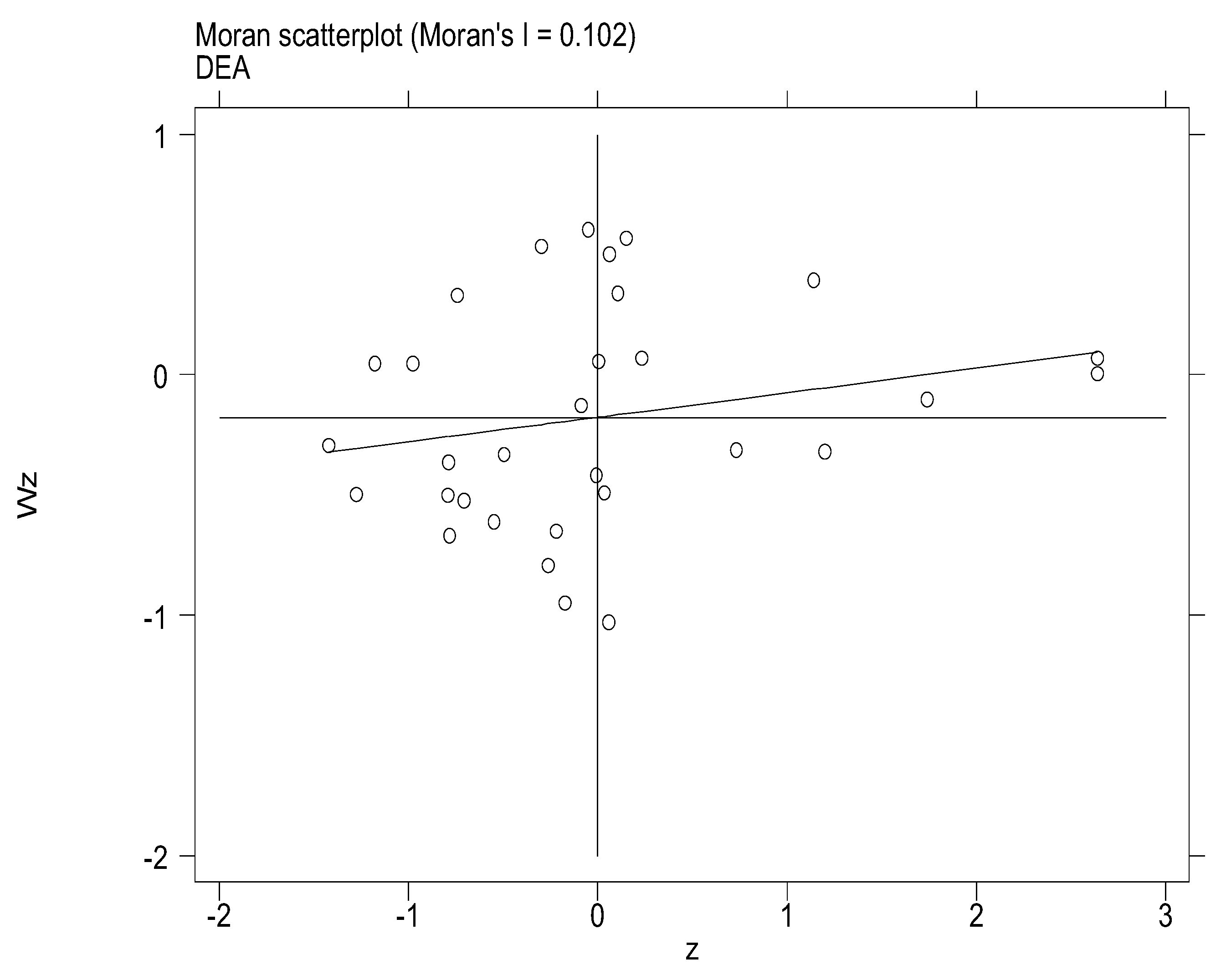
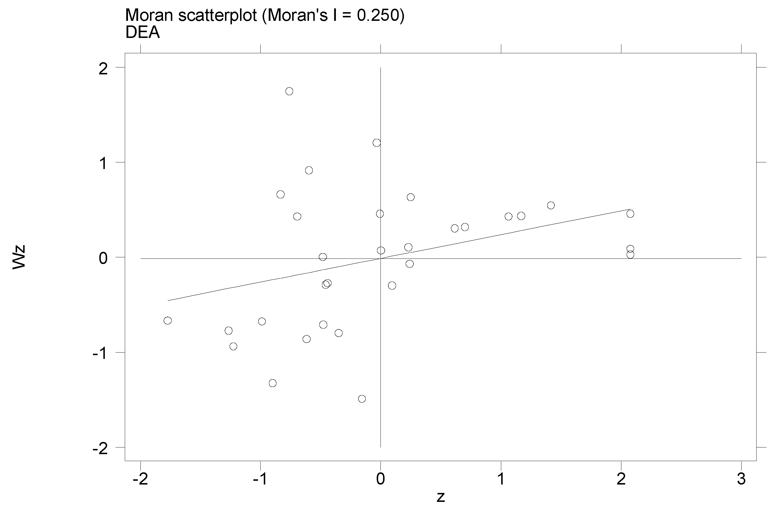
Moran’s I	0.09	0.14 **	0.11 *	0.15 **	0.28 ***	0.21 ***	0.28 ***	0.29 ***	0.29 ***	0.29 ***
Geary’s C	0.67 **	0.68 **	0.74 *	1.03	0.83	0.82	0.78	0.73 **	0.76 *	0.78 *

Notes: ***, **, * denote significance at the 1%, 5%, 10% level; the same applies below.

shows the results of Moran’s Index and Geary’s C of regional innovation performance. As can be seen in Table 1, the Moran’s Index of regional innovation performance in all 31 regions in China is above zero, indicating that there is a positive correlation among regions and the positive correlation level is increasing. From the results of significance test, the Moran’s Index of regional innovation performance is significant except in 2006, and since 2008, Moran’s Index has passed the significance test of 1% level. The results of Geary’s C and Moran’s Index are roughly the same as Moran’s Index. In general, the regional innovation performance of China’s 31 regions shows a significant positive spatial correlation.

Moran scatterplots can show the spatial correlation in all regions more directly. The Moran scatterplot is divided into four quadrants by the horizontal and vertical axes and represents the four kinds of spatial correlations respectively. The first quadrant indcates that the high value observations are surrounded by high value ones. Similarly, the third quadrant indicates the values are also low in the vicinity of the low observed value neighboring areas. And the second quadrant and fourth quadrant indicate that the low-level region is surrounded by the high-value areas and the high-value one is surrounded by the low-value ones, respectively. Due to space limitations, we only list the Moran scatter plots in 2006 and 2015, as shown in Figure 6 and Figure 7. Figure 6 and Figure 7 show that there is a clear positive spatial correlation of innovation performance among the regions which locate in the first quadrant and the third, and the regions with the same high or low regional innovation performance are more likely to gather together.

The results of the spatial correlation test above show that there is a significant positive spatial correlation of regional innovation performance in China. And the results may be biased if we use traditional econometric methods for analysis. Therefore, the spatial econometric model is a better choice to deal with the data which has spatial correlations.

In addition, the panel data needs to be tested for stationarity (unit root test) before the model is estimated. In panel data, when the number of cross-section units is greater than the number of periods, the stationarity of the data will be affected. Unit root test is used before time series modeling or panel data modeling to determine that there is no unit root process in the data. If there are unit roots in the data, that is, the data do not pass the unit root test, it indicates that a pseudo regression may occur during the modeling. If the data is not stable, it will lead to deviation of the estimation results. For this reason, we use the unit root test of LLC (Levin, Lin and Chu) [42] to analyze the stationarity of the data.

As we can see from

Table 2. The results of unit root test.

Variables	$\mathsf{\rho }$	lnGDPP	lnPOP	lnRDP	lnRDC	lnPat	GR	IR	GU	IU
t-value	−15.69	−7.03	−8.69	−14.14	−9.88	−10.10	−9.75	−14.10	−9.06	−10.46
p > t	0.00	0.00	0.00	0.00	0.00	0.00	0.00	0.00	0.00	0.00
Results	Stable	Stable	Stable	Stable	Stable	Stable	Stable	Stable	Stable	Stable

, all of the indicators used in this paper have passed the unit root test; it means that the data is suitable for panel data modeling and that there are no spurious regression problems in the model. The ‘stable’ in Table 2 means that the data have passed the unit root test, that is, the data can be used for spatial econometric model of panel data. In the next part, we will analyze the spatial econometric model from static aspect and dynamic aspect respectively.

5. Results and Discussion

5.1. The Results of Static Panel Data Spatial Econometric Model

Due to the possibility of endogeneity in the spatial econometric model, we use the spatial panel maximum likelihood estimation method (MLE) instead of using the ordinary least-squares estimation method according to Anselin and Elhorst [36,43]. The software we use is stata12.0. Based on the model choice principle of Anselin et al. [44] and the results of Hausman test, the Spatial Autocorrelation Model (SAR) of fixed effect (FE) is selected as the final report result. In addition, considering the influence of collaborative innovation may be lagging, we add both the current and lagged variables of collaborative innovation among IUR into the model. Moreover, in order to ensure the robustness of the estimation method, we also use the GMM (Generalized Method of Moments) method to estimate the model and compare it with the MLE estimation results. At the same time, in order to ensure the robustness of the model index, this paper constructs two kinds of spatial weight matrix, one is R&D Capital Weight Matrix and the other is R&D Personnel Weight Matrix. In summary, the static panel space measurement model results are shown in the following

Table 3. The results of static panel data spatial econometric model.

Variables	R&D Capital Weight Matrix			R&D Personnel Weight Matrix
	MLE-SAR	MLE-SAR-FE	GMM	MLE-SAR	MLE-SAR-FE	GMM
$\mathsf{\rho }$	0.0003 *** (0.0000)	0.0003 *** (0.0000)	-	0.0002 *** (0.000)	0.0002 *** (0.0000)	-
GR	−0.1659 *** (0.0634)	−0.1438 * (0.0774)	−0.1426 * (0.0794)	−0.1342 ** (0.0598)	−0.0938 (0.0728)	−0.1577 ** (0.0800)
L.GR		0.0173 (0.0800)	−0.0541 (0.0830)	-	−0.0188 (0.0751)	−0.0338 (0.0839)
IR	−0.1180 (0.1518)	−0.3224 ** (0.1644)	−0.3752 ** (0.1745)	−0.1575 (0.1424)	−0.3505 ** (0.1536)	−0.3723 ** (0.1745)
L.IR	-	0.4672 *** (0.1701)	0.3360 * (0.1763)	-	0.4173 *** (0.1590)	0.4382 ** (0.1777)
GU	−0.1669 (0.1375)	−0.1421 (0.1538)	0.0931 (0.1600)	−0.0762 (0.1265)	−0.0765 (0.1429)	0.0961 (0.1585)
L.GU	-	−0.0362 (0.1602)	0.1242 (0.1608)	-	0.0088 (0.1487)	0.1165 (0.1593)
IU	−0.1099 (0.1310)	−0.2183 (0.1587)	0.0230 (0.1678)	0.0179 (0.1212)	−0.1314 (0.1483)	0.0057 (0.1698)
L.IU	-	0.1407 (0.1648)	0.3333 ** (0.1652)	-	0.2096 (0.1528)	0.3520 ** (0.1652)
lnGDPP	0.1854 *** (0.06312)	0.1946 *** (0.0624)	0.1897 *** (0.0731)	0.1276 *** (0.0590)	0.1429 *** (0.0581)	0.2055 *** (0.0739)
lnPOP	0.1216 *** (0.0456)	0.1202 *** (0.0447)	−0.0237 *** (0.0492)	0.0514 (0.0390)	0.0526 (0.0383)	−0.0162 (0.0500)
lnRDP	−0.1873 *** (0.0585)	−0.1765 *** (0.0584)	−0.1473 *** (0.0616)	−0.2741 *** (0.0568)	−0.2698 *** (0.0565)	−0.1286 ** (0.0612)
lnRDC	−0.8792 *** (0.0651)	−0.8917 *** (0.0641)	−0.8221 *** (0.0706)	−0.7126 *** (0.0633)	−0.7203 *** (0.0619)	−0.8277 *** (0.0692)
lnPat	0.8555 *** (0.0303)	0.8538 *** (0.0304)	0.8869 *** (0.0352)	0.7928 *** (0.0301)	0.7888 *** (0.0301)	0.8783 *** (0.0355)
constant	0.0737 (0.2869)	0.0170 (0.2972)	0.2308 (0.3506)	0.3857 (0.2656)	0.3109 (0.2761)	0.1531 (0.3581)
Adjust R2	0.5952	0.5985	0.7404	0.5246	0.5235	0.7387

Notes: Standard Error is in the brackets; MLE-SAR represents the spatial autocorrelation (SAR) model estimated by the maximum likelihood estimation (MLE) method, MLE-SAR-FE represents the SAR fixed effect (FE) model estimated by the MLE method, GMM represents the model estimated by GMM method; the same applies below.

.

It can be seen from the table above that the estimation results of the GMM method are basically the same as those of the MLE method, and the estimation results of the R&D Capital Weight Matrix and R&D Personnel Weight Matrix are basically the same, which mean that estimation methods and index selection in the model are robust. The following article analyzes the fixed-effect SAR model results estimated by MLE. The spatial autocorrelation coefficients of R&D Capital Weight Matrix and R&D Personnel Weight Matrix are 0.0002 and 0.0003, respectively, and pass the test at the significance level of 1%. As mentioned above, the innovative elements of R&D personnel and R&D capital contain a great deal of knowledge and information about technological innovation. The dynamic flow between the regional innovation systems facilitates the dissemination and application of knowledge information, which in turn promotes inter-regional knowledge spillover effect. In addition, the dynamic flow of innovation elements such as R&D personnel and R&D capital can also improve the scale of regional innovation systems and optimize the allocation efficiency of elements, which all contribute to the improvement of regional innovation performance. The reason for the value of $\mathsf{\rho }$ being very close to zero is that $\mathsf{\rho }$ is the regression coefficient of regional innovation performance $\theta$, which is measured by DEA method and ranges from 0 to 1. So the coefficient of $\theta$ is generally small, while the size of $\mathsf{\rho }$ has no effect on the significance of it. The relationship of regional innovation performance among different regions as well as the relationship between regional innovation performance and its one period lagging variables are significantly related.

We can see from the four indicators which characterize the synergy of IUR that the current period of government funding and industry funding to universities or research institutes have a negative impact on regional innovation performance. However, the lagged period has a significant positive impact, which indicates that collaborative innovation in IUR is a long process. The cooperation of IUR takes a great deal of time for each part to determine the coordination goal, coordinate resources, and ultimately achieve the innovation goals. However, the current funding of government and industry often cannot directly produce innovation performance, which will have a negative impact on regional innovation performance. On the other hand, industries often prefer to support those scientific research projects with short cycles, low risk and quick returns. They hope to see the benefits in the short term, which lead to innovation cooperation lack of depth and durability and have a negative impact on the overall regional innovation performance. Among several control variables, the coefficients of lnGDPP, lnPOP and lnPat are all significantly positive, which shows improvement of regional economic and development level are all conducive to promoting regional innovation performance.

5.2. The Results of Dynamic Panel Data Spatial Econometric Model

We use a dynamic spatial econometric model to control the endogeneity of the explained variable, and estimate the models in Formulas (3) and (4). The results of the dynamic panel data spatial econometric model are shown in

Table 4. The results of dynamic panel data spatial econometric model.

Variables	R&D Capital Weight Matrix			R&D Personnel Weight Matrix
	SAR	SAR	SAR-FE	SAR	SAR	SAR-FE
$\mathsf{\rho }$	0.0003 ** (0.0001)	0.0004 ** (0.0002)	0.0003 (0.0002)	0.0002 *** (0.0001)	0.0003 *** (0.0001)	0.0002 (0.0001)
L.DEA	0.9344 *** (0.2170)	0.8114 *** (0.1389)	0.8430 *** (0.1686)	0.9261 *** (0.2132)	0.7750 *** (0.1251)	0.8065 *** (0.1387)
GR	−0.0344 (0.0624)	−0.0116 (0.0657)	0.0082 (0.0704)	−0.0237 (0.0614)	−0.0045 (0.0654)	0.0015 (0.0707)
L.GR	-	−0.0230 (0.0631)	0.0037 (0.0678)		−0.0144 (0.0631)	0.0009 (0.0679)
IR	−0.2698 ** (0.1244)	−0.1455 (0.1344)	−0.1522 (0.1442)	−0.2590 ** (0.1226)	−0.1554 (0.1338)	−0.1406 (0.1440)
L.IR	-	0.3059 ** (0.1319)	0.2974 ** (0.1401)		0.2988 ** (0.1312)	0.3011 ** (0.1400)
GU	−0.3173 *** (0.1235)	−0.2542 ** (0.1286)	−0.3085 ** (0.1431)	−0.3113 ** (0.1217)	−0.2500 * (0.1282)	−0.2661 * (0.1422)
L.GU		−0.0832 (0.1287)	−0.0983 (0.1389)		−0.0592 (0.1276)	−0.0905 (0.1392)
IU	−0.3958 *** (0.1379)	−0.3224 ** (0.1470)	−0.3965 ** (0.1581)	−0.3650 *** (0.1350)	−0.3149 ** (0.1460)	−0.3654 ** (0.1597)
L.IU		−0.0135 (0.1360)	−0.0509 (0.1484)		0.0172 (0.1344)	−0.0373 (0.1487)
lnGDPP	0.3167 * (0.1722)	0.0069 (0.2122)	0.1913 (0.2371)	0.2885 * (0.1616)	0.0998 (0.2122)	0.0468 (0.2590)
lnPOP	0.3303 ** (0.1320)	0.7345 *** (0.2831)	0.6061 (0.9654)	0.2438 ** (0.1158)	0.4718 ** (0.2255)	0.5463 (0.9710)
lnRDP	−0.4821 *** (0.0466)	−0.4846 *** (0.0459)	−0.4957 *** (0.0491)	−0.4918 *** (0.0462)	−0.4864 *** (0.0459)	−0.4986 *** (0.0491)
lnRDC	−0.5451 *** (0.0963)	−0.6030 *** (0.1104)	−0.5473 *** (0.1297)	−0.5103 *** (0.0870)	−0.5618 *** (0.1067)	−0.6090 *** (0.1317)
lnPat	0.7755 *** (0.0504)	0.7266 *** (0.0574)	0.7356 *** (0.0606)	0.7574 *** (0.0494)	0.7323 *** (0.0567)	0.7261 *** (0.0621)
constant	−0.1664 (0.1335)	−0.1134 (0.0777)	−0.3542 (0.8663)	−0.0953 (0.1359)	−0.0912 (0.0892)	−0.1690 (0.6422)
Adjust R2	0.6403	0.6208	0.5899	0.6575	0.6285	0.5876

. From the table below we can see that the lagged period of the explained variables all passed the significance test, indicating that there are indeed accumulation effects and inertia effects in innovation production. Previous scientific and technological activities would have an impact on the innovation performance in the current period. The effect of synergy of IUR on regional innovation performance is basically consistent with the results of the static panel model. The co-innovation variables of the current period will have a negative impact on the regional innovation performance, while the lagged one of the co-innovation variables will have a positive impact on the regional innovation performance. These conclusions are consistent with the previous analysis, indicating that the use of dynamic spatial panel econometric model, adding the lagged term of the explanatory variables does not change the conclusion of static panel model, and the results of the model are robust.

6. Conclusions and Recommendations

Based on the panel data of 31 provinces in China from 2006 to 2015, we use spatial econometrics models to analyze the relationships among regional innovation performance, IUR collaborative innovation and spatial correlation by measuring regional innovation performance, constructing R&D Personnel Weight Matrix and R&D Capital Weight Matrix and the synergy index of IUR cooperation. The main findings are as follows:

In terms of policies, firstly, encouraging the government to further increase government investment in R&D innovation and give full play to its guiding role will help promote regional innovation performance. Secondly, strengthening the construction of a collaborative innovation platform for IUR, improving the institutional environment for collaborative innovation, fully mobilizing the enthusiasm of all innovation subjects in participating in collaborative innovation, and giving full play to their respective advantages, will also help enhance the improvement of regional innovation performance. Thirdly, through the establishment of a diversified and competitive financial intermediation system, the functions of R&D resources allocation of financial institutions should be further optimized so as to make them more integrated into the collaborative innovation system and provide more opportunities for industries and research institutions.

Both the coefficients of R&D Personnel Weight Matrix and R&D Capital Weight Matrix are significantly positive, which means that there is a spatial spillover effect and a significant spatial positive correlation among different regions. To a certain extent, this shows that the flow of R&D personnel and R&D capital among different regions can help to promote the spillover effect of regional innovation performance. This conclusion shows that further strengthening the decisive role of the market in the allocation of resources, breaking down institutional barriers to the flow of innovative elements such as R&D personnel and R&D capital, and striving to create an external environment conducive to the flow of innovative elements will improve overall regional innovation performance. In addition, to further improve the benefits and working conditions of R&D personnel and to broaden the investment channels of R&D capital will help the region to attract more R&D personnel and R&D capital so as to expand its production scale, improve its structure and promote the development of regional innovation activities.

References

- The Central People’s Government of the People’s Republic of China. The Guideline on Strengthening the Core Status of Enterprise Technology Innovation and Improve Enterprise Innovation Ability Comprehensively. Available online: http://www.gov.cn/zwgk/2013-02/04/content_2326419.htm (accessed on 6 April 2018).
- Bonaccorsi, A.; Piccaluga, A. A theoretical framework for the evaluation of university-industry relationships. R D Manag. 1994, 24, 229–247. [Google Scholar] [CrossRef]
- Perkmann, M.; Neely, A.; Walsh, K. How should firms evaluate success in university–industry alliances? A performance measurement system. R D Manag. 2011, 41, 202–216. [Google Scholar] [CrossRef]
- Pertuze, J.A.; Calder, E.S.; Greitzer, E.M.; Lucas, W.A. Best practices for industry-university collaboration. MIT Sloan Manag. Rev. 2010, 51, 83–90. [Google Scholar]
- Bolling, M.; Eriksson, Y. Collaboration with society: The future role of universities? Identifying challenges for evaluation. Res. Eval. 2016, 25, 209–218. [Google Scholar] [CrossRef]
- Bonaccorsi, A.; Colombo, M.G.; Guerini, M.; Rossi-Lamastra, C. University specialization and new firm creation across industries. Small Bus. Econ. 2013, 41, 837–863. [Google Scholar] [CrossRef]
- D’Este, P.; Iammarino, S. The spatial profile of university-business research partnerships. Papers Reg. Sci. 2010, 89, 335–350. [Google Scholar] [CrossRef]
- Muscio, A.; Nardone, G. The determinants of university-industry collaboration in food science in Italy. Food Policy 2012, 37, 710–718. [Google Scholar] [CrossRef]
- Bigliardi, B.; Galati, F.; Marolla, G.; Verbano, C. Factors affecting technology transfer offices’ performance in the Italian food context. Technol. Anal. Strateg. Manag. 2015, 27, 361–384. [Google Scholar] [CrossRef]
- Maietta, O.W. Determinants of university-firm R & D collaborative and its impact on impact on innovation: A perspective from a low-tech industry. Res. Policy 2015, 44, 1341–1359. [Google Scholar]
- Guan, J.; Liu, S. Comparing regional innovative capacities of PR China based on data analysis of the national patents. Int. J. Technol. Manag. 2005, 32, 225–245. [Google Scholar] [CrossRef]
- Wu, J.; Zhou, Z.X.; Liang, L. Measuring the performance of Chinese regional innovation systems with two-stage DEA-based model. Int. J. Sustain. Soc. 2010, 2, 85–99. [Google Scholar] [CrossRef]
- Guan, J. Measuring the Efficiency of China’s Regional Innovation Systems: Application of Network Data Envelopment Analysis (DEA). Reg. Stud. 2012, 46, 355–377. [Google Scholar]
- Aghion, P.; Howitt, P. On the Macroeconomic Effects of Major Technological Change. Ann. Decon. Stat. 1998, 3, 53–75. [Google Scholar] [CrossRef]
- Kim, C.S.; Inkpen, A.C. Cross-border R & D alliances, absorptive capacity and technology learning. J. Int. Manag. 2005, 11, 313–329. [Google Scholar]
- Maurer, I.; Bartsch, V.; Ebers, M. The Value of Intra-Organizational Social Capital: How It Fosters Knowledge Transfer, Innovation Performance, and Growth. Organ. Stud. 2011, 32, 157–185. [Google Scholar] [CrossRef]
- Mowery, D.C.; Sampat, B.N. Universities in National Innovation Systems; Oxford Handbook of Innovation; Oxford University Press: Oxford, MS, USA, 2005. [Google Scholar]
- Metcalfe, S.; Ramlogan, R. Innovation systems and the competitive process in developing economies. Q. Rev. Econ. Financ. 2008, 48, 433–446. [Google Scholar] [CrossRef]
- Cooke, P. Regional Innovation Systems: General Findings and Some New Evidence from Biotechnology Clusters. J. Technol. Transf. 2002, 27, 133–145. [Google Scholar] [CrossRef]
- Arvanitis, S.; Kubli, U.; Woerter, M. University-industry knowledge and technology transfer in Switzerland: What university scientists think about co-operation with private enterprises. Res. Policy 2008, 37, 1865–1883. [Google Scholar] [CrossRef]
- Bernard, A.; Jones, A. Technology and Convergence. Econ. J. R. Econ. Soc. 1995, 106, 1037–1044. [Google Scholar] [CrossRef]
- Kallio, A.; Harmaakorpi, V.; Pihkala, T. Absorptive capacity and social capital in regional innovation systems: The case of the Lahti region in Finland. Urban Stud. 2010, 47, 303–319. [Google Scholar] [CrossRef]
- Azagra-Caro, J.M.; Archontakis, F.; Gutierrez-Gracia, A.; Fernandex-de-Lucio, I. Faculty support for the objectives of university-industry relations versus degree of R & D cooperation: The importance of regional absorptive capacity. Res. Policy 2006, 35, 37–55. [Google Scholar]
- Lai, I.K.; Lu, T.W. How to improve the university-industry collaboration in Taiwan’s animation industry? Academic vs. industrial perpectives. Technol. Anal. Strateg. Manag. 2016, 28, 717–732. [Google Scholar] [CrossRef]
- Jung, J.; López-Bazo, E. Factor Accumulation, Externalities, and Absorptive Capacity in Regional Growth: Evidence from Europe. J. Reg. Sci. 2017, 57, 266–289. [Google Scholar] [CrossRef]
- Escribano, A.; Fosfuri, A.; Tribo, J.A. Managing external knowledge flows: The moderating role of absorptive capacity. Res. Policy 2009, 38, 96–105. [Google Scholar] [CrossRef]
- Miguélez, E.; Moreno, R. Knowledge flows and the absorptive capacity of regions. Res. Policy 2015, 44, 833–848. [Google Scholar] [CrossRef]
- Li, X. China’s regional innovation capacity in transition: An empirical approach. Res. Policy 2009, 38, 338–357. [Google Scholar] [CrossRef]
- Li, J.; Tan, Q.; Bai, J. Spatial Econometrics Analysis of China Regional Innovation Technology. Manag. World 2010, 7, 43–65. (In Chinese) [Google Scholar]
- Shi, X.; Zhao, S.; Wu, F. Analysis of Regional Innovation Efficiency and Spatial Discrepancy in China. J. Quant. Techn. Econ. 2009, 3, 45–55. (In Chinese) [Google Scholar]
- Zhang, Y.; Li, K. Research on the Spatial Dependence of Chinese Province-Level Innovation Output. Stud. Sci. Sci. 2008, 26, 659–665. (In Chinese) [Google Scholar]
- Li, J.; He, Y. Study of Knowledge Spillover Effect on Regional Innovation Performance from the Perspective of Spatial Correlation—Based on provincial Data Samples. R D Manag. 2017, 29, 42–54. (In Chinese) [Google Scholar]
- Bai, J.; Jiang, F. Synergy Innovation, Spatial Correlation and Regional Innovation Performance. Econ. Res. J. 2015, 7, 174–187. (In Chinese) [Google Scholar]
- Paelinck, J.; Klaassen, L. Spatial Econometrics; Saxon House: Farnborough, Hampshire, UK, 1979. [Google Scholar]
- Anselin, L.; Varga, A.; Acs, Z. Local Geographic Spillovers between University Research and High Technology Innovations. J. Urban Econ. 1997, 42, 422–448. [Google Scholar] [CrossRef]
- Anselin, L. Spatial Econometrics: Methods and Models; Kluwer Academic Publishers: Dordrecht, The Netherlands, 1988. [Google Scholar]
- Getis, A.; Griffith, D.A. Comparative Spatial Filtering in Regression Analysis. Geogr. Anal. 2002, 34, 130–140. [Google Scholar] [CrossRef]
- Fischer, M.M.; Varga, A. Spatial knowledge spillovers and university research: Evidence from Austria. Ann. Reg. Sci. 2003, 37, 303–322. [Google Scholar] [CrossRef]
- Smith, S.L.J. Tourism Analysis: A Handbook; Longman: Harlow, UK, 1989. [Google Scholar]
- Witt, S.F.; Witt, C.A. Forecasting tourism demand: A review of empirical research. Int. J. Forecast. 1995, 11, 447–475. [Google Scholar] [CrossRef]
- Roy, J.R.; Thill, J.C. Spatial Interaction Modelling; Springer: Heidelberg/Berlin, Germany, 2004. [Google Scholar]
- Levin, A.; Lin, C.F.; Chu, C.S.J. Unit root tests in panel data: Asymptotic and finite-sample properties. J. Econom. 2002, 108, 1–24. [Google Scholar] [CrossRef]
- Elhorst, J.P. Specification and Estimation of Spatial Panel Data Models. Int. Reg. Sci. Rev. 2003, 26, 244–268. [Google Scholar] [CrossRef]
- Anselin, L.; Bera, A.K.; Florax, R.; Yoon, M.J. Simple diagnostic tests for spatial dependence. Reg. Sci. Urban Econ. 1996, 26, 77–104. [Google Scholar] [CrossRef]