Abstract
Quantifying the impact of the application of sustainable transport policies is essential in order to mitigate effects of greenhouse gas emissions produced by the transport sector. One of the most common approaches used for this purpose is that of traffic modelling and simulation, which consists of emulating the operation of an entire road network. This article presents the results of fitting 8 well known data science methods for transport choice modelling, the area in which more research is needed. The models have been trained with information from Biscay province in Spain in order to match as many of its commuters as possible. Results show that the best models correctly forecast more than 51% of the trips recorded. Finally, the results have been validated with a second data set from the Silesian Voivodeship in Poland, showing that all models indeed maintain their forecasting ability.
1. Introduction
Transport systems performance evaluation and forecasting is a difficult task currently under consideration by many research centers. This complexity emerges mainly due to its stochastic nature, whereby a large number of variables and personal preferences come into play [1]. Transport infrastructures are highly expensive and if the solution does not fit the necessities of the citizens, the infrastructure might need to be upgraded, increasing the cost or, even worse, becoming a worthless investment [2]. Therefore, a cheap and flexible method for testing future transport developments is to use computer simulations supported by advanced mathematical models [3].
To calculate the impact of the transport sector, traditional approaches are relying on simulations, a paradigm that has become a popular and effective technique to analyze a wide range of dynamically changing systems. The essence of simulating is to carry out a series of computational experiments using a model that describes the operations of the real system (how drivers, vehicles, signals, pedestrians, etc. interact) and to generate output data that characterizes the subject system [4]. Traffic simulation allows one to check, monitor, and evaluate the behavior of the real systems under different realistic conditions in an artificial-computer-based environment [5]. Most common traffic simulations focus on simulating everyday traffic activity in search of congestions, assessing different ways of enabling traffic in intersections (crossings, roundabouts, traffic lights, etc.) or applying dynamic speed limits to avoid jams.
Over the last decades, many universal approaches have been widely used for modeling stochastic processes, such as Monte Carlo techniques [6], Markov chain models [7], or queuing theory methods [8]. Today’s state-of-the-art simulation packages (listed later) add features such as graphical interfaces and object-oriented programming and even allow one to simulate both continuous and discrete events. Regarding transport simulation, two mutually interrelated pieces of information are needed [9]: the demand that characterizes the need for movement (passengers or freight) and a description of the transport network, traffic zones, and vehicles. By combining these data sets, state-of-the-art models follow the standard concept of the four-step model (FSM) [10]. FSM is a primary tool for the analysis of transport systems, assessment of their performance, and prediction of their future behavior. This model is composed of the following phases:
- Trip generation: Generate a specific, whether fixed or approximated, amount of vehicles that represents the population.
- Trip distribution: Spread the population along the scenario in a realistic distribution.
- Transport choice: Schedule their transport mode and itineraries throughout the city to reach their destination.
- Traffic simulation: Estimate the global impact derived from the configuration of a single scenario and compare the results with those obtained from others.
In this sense, multi-agent systems (MASs) have been an active area of research in the last three decades [11]. What started as isolated systems for simple problem-solving has turned into full-scale simulation platforms that are able to integrate several state-of-the-art technologies. Specially, for transport systems evaluation, agent-based simulation models have been proven to be very useful [12]. In these models, each vehicle is represented as a software object, a so-called intelligent agent, that has its own set of parameters and attributes that define how the agent will behave, interact, make decisions, and communicate with the other agents in the system [13]. This approach allows one to build a thoroughly detailed description of the model population. According to their accuracy and scope, simulation models can be classified as follows:
- Micro-simulation models: These models describe traffic with a high level of detail and distinguish separate elements in the traffic flow, such as types of vehicles and pedestrians. Though the use of this high level of detail entails very precise analysis, it must be limited to a small area or intersection due to its complexity. The most popular micro-simulation tools are PTV Vissim [14], Aimsun [15], and Corsim [16].
- Meso-simulation models: These models describe traffic with an intermediate level of detail, distinguishing separate elements in the traffic flow but not taking into account the interactions between them. They are less precise and can be applied to cover larger areas than those of the micro-simulation. The most popular meso-simulation tools are Dynasmart [17] and Transims [18].
- Macro-simulation models: These models describe traffic with a high level of aggregation, as a uniform traffic flow. They are based on deterministic relationships between the parameters characterizing the traffic flow, such as volume, speed, or density. Macroscopic simulation has been developed to model an entire transport network and/or system. The most popular macro-simulation tools are Emme/2 [19], PTV Visum [20], and Transcad [21].
A great amount of research effort has been put into understanding transport mode choice modeling and how the travelers’ background, trips and transport facilities influence the attractiveness of transport [22]. The evaluation of transport systems depends completely on how people adapt to it. This implies modeling social preferences that have particular importance when traveling, such as time, cost, comfort, or environment-friendly awareness. Even as the aforementioned simulators are relatively easy to run and have many proven success stories, most focus primarily on the calculation and estimation of routes and congestion avoidance, leaving out the social behavior that influences the traveler’s choice of using one transport method or another.
For those simulators that model transport selection, discrete choice regression models (probit and logit models) [23] are the most widespread techniques [24]. In fact, the three simulators that include transport choice models (Aissum, TRANSIMS, and TransCAD) implement these types of models. However, the addition of new transport modes, the alteration of the transport network, or the evaluation of the application of new incentives and restrictions requires calibrating (and sometimes building) the entire model again.
Within this scope, this article compares eight methodologies to model human decision making when choosing between transport modes. The objective is to emphasize the models that perform better and assess the difficulty of extending them to assess the introduction of new policies or transport methods. All models will be trained with a real data set, and their results will be validated with another data set. This process is of great importance for analyzing the impacts that sustainable transport policies will have when applied over the specific geographical and demographic characteristics of a certain area.
The rest of the paper is organized as follows. Section 2 describes the materials used and details of the proposed transport choice methodologies. Section 3 presents and analyzes the results derived from the application of these methodologies to two different scenarios. The final section presents the conclusions and discussion that emerge from the analysis of the results.
2. Materials and Methods
In order to better understand the methodology presented, the next subsections will detail its implementation according to the stages defined in the FSM.
2.1. Trip Generation and Distribution
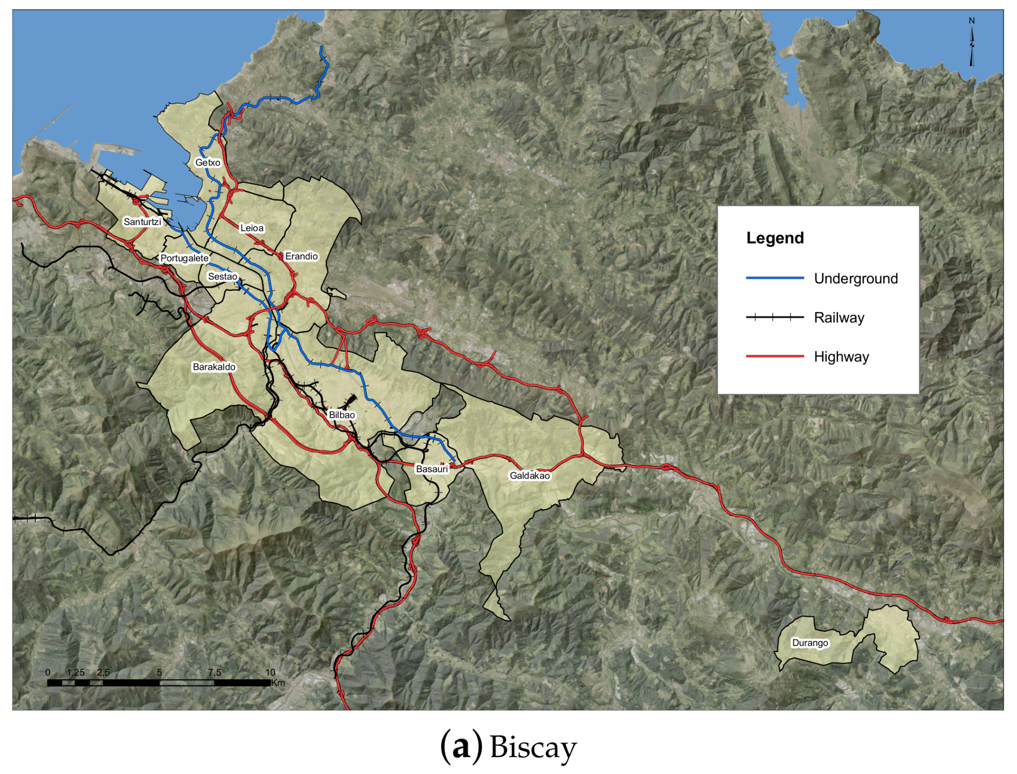
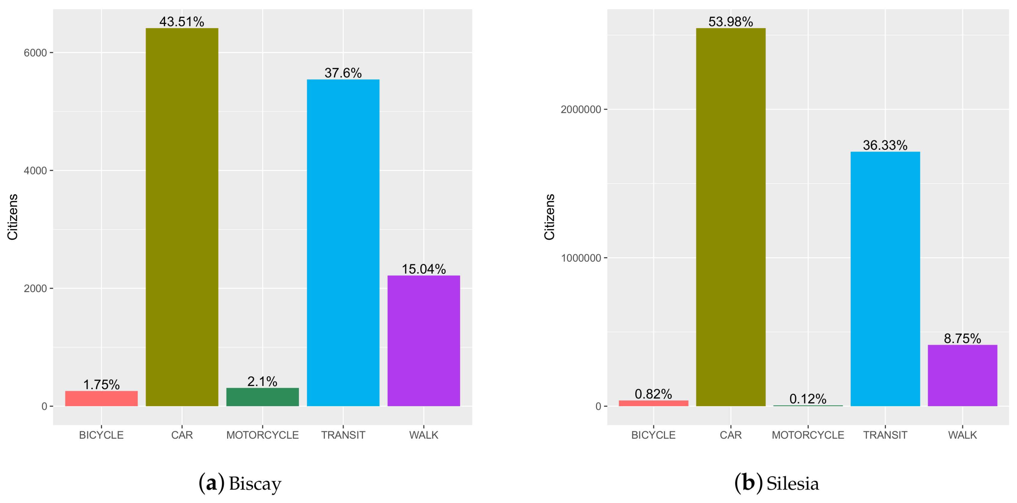
In order to generate the information to train the models, agent-based simulations were extensively used. The main characters of the simulation are the citizens, where each citizen agent has a set of personal preferences that will directly influence the transport choice for traveling. For the generation and distribution of the trips for the experimentation, two data sets were used. On the one hand, Biscay’s commute data (depicted in Figure 1a and Figure 2a) was extracted from the census performed every 10 years by the Spanish National Statistics Institute [25]. This data set covers the region of Biscay, in the Basque Country, with an area of 2217 km2. The census also details the points of origin and destination of traveling for the most populated 11 municipalities of the region, with a total population of about 1,100,000 citizens. This data set will be used to train the different models. On the other hand, Silesia commutes (depicted in Figure 1b and Figure 2b) were extracted from the green traveling project’s surveys [26]. The data set covers 19 municipalities of the central part of Silesian Voivodeship with a population of 4,710,000 citizens. This data set will be used to validate the results.

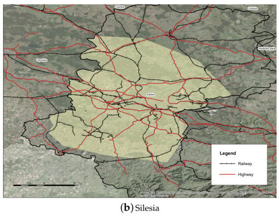
Figure 1.
Area and transport links of Biscay (Spain) and Silesia (Poland) data sets. Source: own research generated from real boundaries and transport networks.
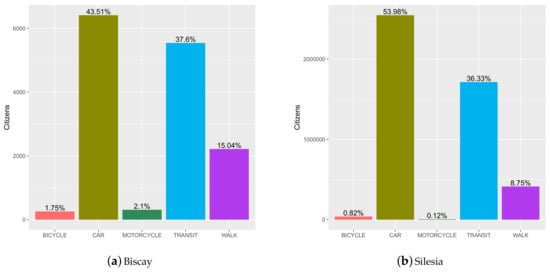
Figure 2.
Modal splits for the Biscay and Silesia data sets. Source: own research from the datasources of [25,26].
When the data set is brought to life by the simulation, each citizen agent registers its point of origin, point of destination, departure time, and the itinerary for the five transport modes. The platform preprocesses the input data to geolocate each citizen agent on the environment through a weighted distribution. This process assigns the origin of each citizen agent to household buildings in the municipality and the destination to available amenities, commercial, or industrial buildings. The weighted distributions are based on the buildings’ size and levels, i.e., the bigger and the taller the building, the higher the probability of assigning a citizen agent to it. Once located, citizens will calculate the five itineraries for CAR, MOTORCYCLE, TRANSIT, BICYCLE, and WALK. For each itinerary, the main characteristics of every choice (see Section 2.2 for details) will be stored in order to build their decision process. Some itineraries might be null due to a lack of public transport stop nearby or an inability to calculate the route.
2.2. Transport Mode Choice
There are many features that determine the modal split of a territory. More than 45 years ago, the authors of [27] identified the main features that influence commuters’ choices, and since then other important characteristics have been added to the list [28]. In spite of using different techniques, researchers agree that itinerary dependent variables can be grouped into four main categories that represent the physical and factual features of a trip [29]: duration, price, length, and environmental impact. Table 1 describes these categories and shows how they are usually further divided in other second-level features. Nonetheless, these four variables do not cover some other features listed in the literature, which are directly linked to the traveler’s background. These background variables, presented in Table 2 do not appear in the census nor in the surveys and are therefore beyond the scope of this study (see Section 4 for details).

Table 1.
Itinerary features used for transport choice. Source: Adapted from [29].

Table 2.
Itinerary features are not present in the data sets and are beyond the scope of the study. Source: own research, conducted by analyzing the features mentioned in [27], which are not present in the data sets.
Missing values have been the main source of problem. In these data sets, missing values appear as NaN (not a number), representing that the itinerary is undefined. There are valid reasons to have missing values in the data set (for example, it is not possible to travel from one place to other using public transport), but a closer look reveals that the missing values are randomly distributed and do not follow any logical pattern (for example, itineraries that can be performed by MOTORCYCLE and not by CAR). This suggests that missing values originated from the routing algorithm time-out errors due to the inability to calculate complex routes. For this reason, all NaN values were replaced with an arbitrary number that was greater than any of the real measured values (in this case, all NaNs were replaced by the maximum value in the data set).
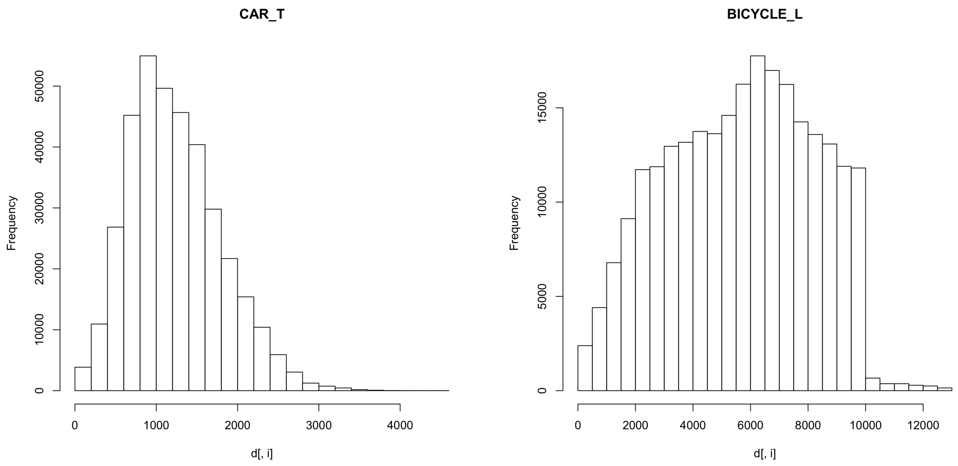
The rest of the variables do not present any obvious problems. In fact, they clearly show an expected distribution. For example, Figure 3 shows the length of the trips made with BICYCLE. As expected, there is a point where the trips using BICYCLE are too costly and fall sharply. Another expected result is, for example, the distribution of time expended in CAR trips. As seen in the left panel of Figure 3, the distribution almost follows a distribution. As citizens tend to be normally geographically distributed [30], the distance traveled follows a distribution, as does the time spent.
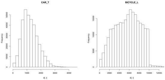
Figure 3.
Distribution of time (left) and length (right) for CAR and BICYCLE transport modes in Silesian Voivodeship.
The influence of these variables on transport choice was modeled through eight modeling techniques: k-nearest neighbors (KNNs) [31], multinomial logit (M) [32], support vector machines (SVMs) [33], neural networks (NNs) [34], naïve Bayes (B) [35], fuzzy logic (CE) [36], expert knowledge (EK) [37], and random search (RA).
2.2.1. Multinomial Logit Models
Following the so-called latent construct interpretation, multinomial models work by adjusting a helper function p that takes as input a vector of external factors that affect the choice and gives as output the selected one. For a two class case, the function p takes the form:
where X is a vector of the variables considered to make the regression, is the vector of regressors to be estimated, and is a random variable following the logistic (logit) or normal (probit) distribution. Details can be consulted in [32].
2.2.2. Support Vector Machines
This technique builds a black-box model that can be tailored for classification and regression problems [33]. A more detailed explanation is beyond the scope of this document and readers interested can consult [33] for details. Since the transport choice is a classification problem, the default approach -classification was followed. This technique features three hyper-parameters: C controls the penalization to the errors in the training sample, controls the margin of tolerance to errors, and controls the bandwidth of the radial function. These hyper-parameters have been optimized using a grid search following the advice given in [38].
2.2.3. Neural Networks
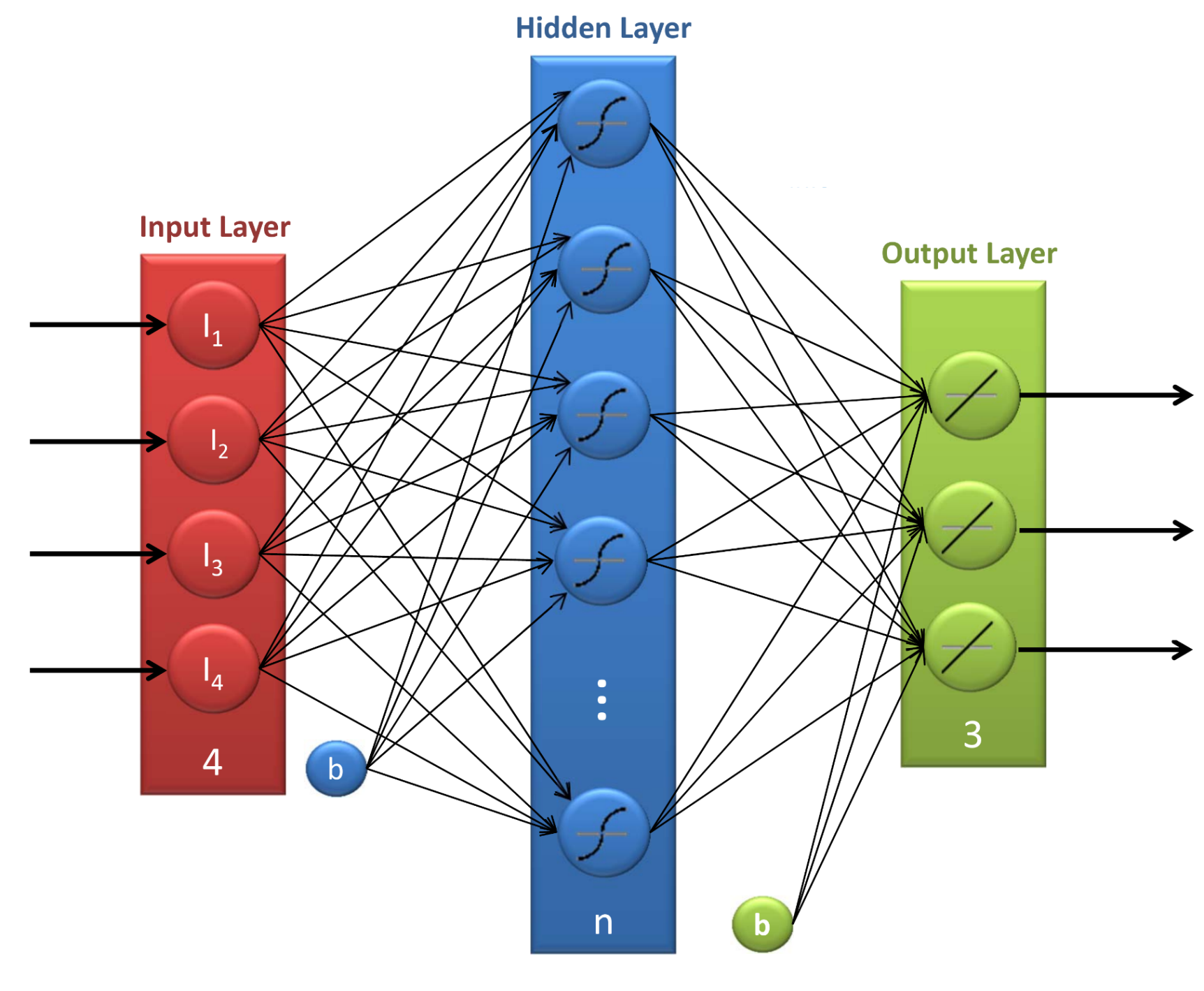
This technique builds a black-box model that tries to mimic the behavior of the natural neurons. This way, a neural network is composed of a set of artificial networks arranged into three layers: an input layer, a hidden layer, and an output layer (see Figure 4). The outputs of one layer are connected to the inputs of the subsequent layers, building in this way a network of neurons. Finally, each neuron computes the following function:
where x is the input vector w, b are the parameters of the model (wights and bias), and denotes the sigmoid function [39]. Further details can be consulted in [34]. The hidden layer features several numbers of neurons, and the parameters of the model have been adjusted through backpropagation.
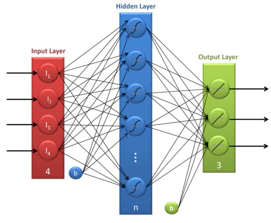
Figure 4.
Structure of a neural network (NN).
The main hyper-parameter of this model is the number of neurons m in the hidden layer. In this case, a grid search has been followed to optimize this value such that is the best value.
2.2.4. The Naïve Bayes (B) model
This model extends Bayes’ theorem to perform classifications. This way, this model estimates a probability of every transport mode given the vector of variables considered to make the prediction X. For this end, the algorithm just needs to calculate an estimation of the probability of X conditional of every transport mode c and then use Bayes’ Theorem. The output class will be the one with the greatest probability. Details of this model can be found in [35].
2.2.5. k-Nearest Neighbours
This method uses the notion of the closeness of the input to perform classifications. This way, given a new element y to classify, the algorithm searches the k-nearest elements known in the training set with respect to a given metric (usually the Euclidean) and classifies y as the weighted mean value of the nearest neighbours (in a regression setting) or the most common class among the k-nearest elements (in a classification setting as this one). Using a grid search procedure, it was found that was the best value for this project.
2.2.6. Fuzzy Logic
All methods presented above are black-box models or are not straightforward in considering new transport modes or new input variables. Fuzzy logic [36], however, has been shown to achieve high success in the emulation of individual preferences for transport mode choice [40,41], therefore enabling a wider level of parametrization for each citizen’s profile. A well trained fuzzy logic engine and accurately defined rule sets are expected to provide consistent results even in the case of variation in the characteristics of the transport network.
Fuzzy logic engines build discrete choice models through a simple natural language rule-based approach [42]. Classical logic only allows conclusions to be true or false. In contrast, fuzzy logic defines a set of rules that map numeric data into linguistic terms and creates fuzzy sets, indicating the extent to which each term is part of. That is, a variable can have several values (called terms) that can be overlapped and shaped. Thereby, it is possible to model how each feature increases or decreases the likelihood of choosing a given transport mode. Fuzzy logic engines are parametrized though their inputs, outputs, and rules. For this research, the fuzzy logic was built as follows:
- Inputs, terms, and membership functions: For the engine to translate from linguistic terms to numbers, inputs are composed of a name that identifies the input, the possible terms or values that the input can take, and a membership function that limits the extent to which each term can be classified. The inputs of the model presented here are built from the four previously mentioned itinerary features: DURATION, PRICE, LENGTH, and ENVIRONMENTAL IMPACT. Each of these inputs feature a fixed set of three terms: LOW, MEDIUM, and HIGH, shaped as triangles. The anchors of these triangles (, , , and ), shown in Figure 5, are key values that describe how citizens understand these qualitative variables.
 Figure 5. Fuzzy engine input membership functions, with the configurable anchors that modify the shape of the terms. Source: own research for better understanding the input membership functions.
 - Outputs, terms, and membership functions: Similarly to the inputs, the outputs are composed of a name that identifies the output, the possible terms or values the output can take, and a membership function for each term. The model presented here features a single output with five fixed, non-overlapping terms that represent the transport modes among which to choose: CAR, MOTORCYCLE, PUBLIC TRANSPORT, BICYCLE, and WALK, as represented in Figure 6.
 Figure 6. Fuzzy engine output. Each term represents a mode of transport one may choose. Source: own research for better understanding the fuzzy logic output membership function.
 - Rules: Rules follow the following structure: if INPUT is INPUT_TERM and … then OUTPUT is OUTPUT_TERM. The engine needs a set of rules, each with one output but with one or more terms, as depicted in Table 3. Additionally, the engine provides fuzzy value modifiers or hedges through natural language keywords to help describe border cases without the need to include additional terms: ANY, NOT, EXTREMELY, SELDOM, SOMEWHAT, or VERY. The defuzzifier will be the maximum value between the three terms, that is, the term that receives the maximum value and thus the one chosen by the citizen. Please note that only AND conjunctions will be used between rule terms, since disjunctions can be represented by splitting a rule in two or using the NOT hedge.
 Table 3. Example of fuzzy engine rule sets. Source: own research for explaining the structure and examples of fuzzy logic rules.
Expert Fuzzy Knowledge (EK)
A first approach of the definition of the fuzzy logic inputs and rules was created according to both literature [37] and internal transport surveys carried out for the green traveling project [43,44]. From this information, a simple set of rules was extracted. These rules can be consulted in Table 4.

Table 4.
Fuzzy engine rule sets extracted from surveys and expert knowledge. Source: own research generated from the surveys in [43,44].
A Co-Evolutionary Fuzzy Logic Algorithm (CE)
While expert knowledge can lead to accurate solutions and is crucial for a better understanding of the problem, it is not flexible enough to variations in the inputs used to build that knowledge. Therefore, it is always advisable to further search whether a better solution can be reached. Trying to manually improve the expert knowledge rules to match a wider number of citizens from the census involves applying many changes to interrelated inputs and rule sets in a very large search space. One of the approaches to automate this is to use an evolutionary algorithm and to divide the search space in subsets of problems.
Genetic programming techniques have already been used to train fuzzy logic models [45]. Here, a cooperative co-evolution programming method (CE) is presented. CE is a form of evolutionary computation method that divides a large problem into sub-components and solves them independently in order to solve the large problem [46]. The sub-components are implemented as sub-populations and the only interaction between sub-populations is in the cooperative evaluation of each individual of the sub-populations. The cooperative evaluation of each individual in a sub-population is done by concatenating the current individual with the best individuals from the rest of the sub-populations. The algorithm presented hereby tackles both the adjustment of the the input linguistic variables membership functions and the search of the rule sets that most faithfully fit the census data. These two variables are strongly related since any change in the input terms’ extent requires adapting the rules to the new meaning of the linguistic variable. Thus, the CE algorithm suits perfectly the problem of the optimizing two interrelated variables in two sub-components:
- Input-evolving sub-component: This is composed of a population of 200 input sets. Each input set features the four input variables already mentioned—DURATION, PRICE, LENGTH, and ENVIRONMENT. Each input has three fixed and ordered terms—LOW, MEDIUM, and HIGH—whose triangle anchors , , , and (see Figure 5 for details) can be modified in search of limits that better fit the citizens’ appreciation for these qualitative terms.
- Rule evolving sub-component: This is composed of a population of 200 rule sets. Each rule set features a list with a variable number of rules, and, for each rule, its terms and output are modified to extract the combination of rules that more faithfully represents citizens’ transport choice from the census.
Each combination of input membership functions and rules defines what is called a fuzzy experiment. On evaluation, each fuzzy experiment configures the fuzzy logic engine to test how accurate the outputs of the engine are compared to the census. On the evolution of the input sets, whenever a change is applied in any of the triangle anchors, a fuzzy experiment will be created with corresponding input set, the fixed output, and the best found rule set to calculate the input set’s fitness. Likewise, on the evolution of the rule sets, whenever a change is applied to the rules (whether it is an addition, a deletion, or a change in the terms), a fuzzy experiment will also be created with a corresponding rule set, and the best input set for calculating its fitness will be found.
Although evolutionary algorithm operators traditionally use mutation and crossover, rule set mutations produce only slight changes in the population. Therefore, a more abrupt approach has been designed by relying only on the crossover operator. The crossover operators for evolving rule sets and evolving input sets are detailed below.
- Operators used for Rules:
- rule set slice crossover Given two rule sets, this operator creates a new rule set, taking the first to n rules from the first set and the n to last rules from the second set.
- rule set combine crossover Given two rule sets, this operator creates a new rule set, appending for each position a randomly selected rule from the same position of the two provided rule sets.
- rule set slice terms crossover Given two rule sets, this operator clones the first rule set and selects a p rule in the set. The p rule’s terms are replaced by the first to n terms from the p rule of the first set and n to last from the p rule of the second provided set.
- Fuzzy Logic Input Membership Functions:
- input set combine crossover Given two input sets, this function creates a new input set, appending for each position a randomly selected element from the same position of the two provided input sets.
- input set shape mutation Given an input set, this function modifies one of the , , , or values from the shapes in Figure 5. It will displace at the same time the first term’s triangle’s third point, the second term’s triangle’s mid-point, and the third term’s triangle’s first point.
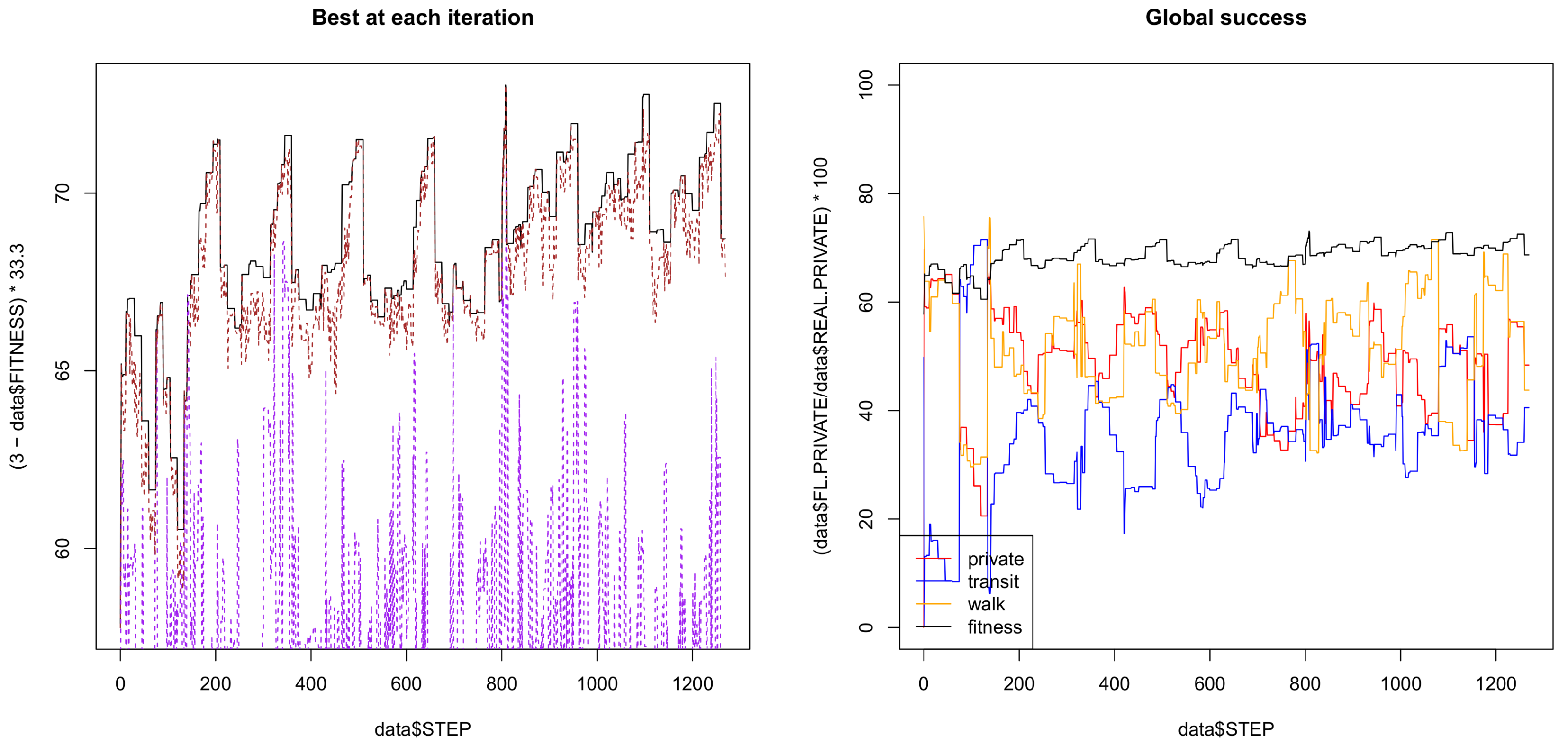
The fitness of a fuzzy experiment is given by the amount of citizens that match the transport choice originally registered in the census (that is, the accuracy of the forecasting model). The goal of the CE algorithm is, therefore, to maximize the fitness in order to estimate as many correct transport choices as possible. For this, a confusion matrix is calculated within each fitness evaluation. Confusion matrices are square matrices with a number of rows and columns equal to the number of output terms. Columns denote the amount of real elements, and rows denote the predicted elements of that class, that is, a column contains a split of 100% of the elements. Namely, cell denotes the percentage of elements classified as i that are of class j. The diagonal of this matrix (namely the elements ) describes the correctly classified elements. For instance, in Table A1, 19.8004% of C (CAR) instances were forecast correctly, but 14.4995% of C users were forecast as M (MOTORCYCLE) users. The global fitness is composed of the best element of the input and rules populations as seen in Figure 7.
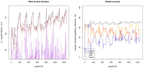
Figure 7.
Iterations of the co-evolutive fuzzy algorithm. Source: own research by plotting the evolution in time of the algorithm.
Since the number of elements for each vehicle type is not balanced, a fuzzy experiment that matched only CAR would obtain a better fitness than other operating on a more distributed modal split. Therefore, the previously defined correctly classified elements has been improved to include balanced correctly classified elements. In this sense, let denote the relative partial matches of class k, namely,
Then, the fitness function f is defined as the sum of the logarithm of the partial matches . Namely,
Please note that we add 1 to the partial matches to avoid undefined values of the fitness function when a model does not correctly classify any element. Thus, with this approximation, not only are all vehicle types balanced, but rules that match the census in a more distributive way also weigh more.
Additionally, a gradually growing subset of the census is used to calculate the fitness. This subset is extended as the matched percentage of that subset increases. That is, the first iteration’s fitness is calculated with a 10% subset of the entire census data set. Following iterations, the subset will be kept equal or increased parallel to the matched percentage. In this way, as matched elements increase, more elements are introduced in the census, against which the next iteration’s fitness can be evaluated. Moreover, in order to go through all the elements of the census, at every 15 iterations, the subset to extract from the census is moved by 10%. This changes in the reference data with which to evaluate the fitness and generates the repeating pattern visible in Figure 7.
As a summary, the pseudo code for the CE algorithm is described in Figure 8. The algorithm is divided into two main procedures:
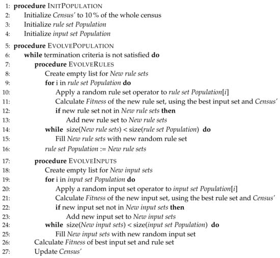
Figure 8.
Pseudocode of the co-evolutionary fuzzy logic algorithm. Source: own research simplification of the real code programmed in the algorithm.
- initialize the population of rule sets and input sets that will take part in the co-evolutionary process, and
- initialize the co-evolutionary process itself where the rule sets and input sets evolve together through the application of the evolutionary operators, the calculation of the fuzzy experiments’ fitness on each iteration, and the update of the percentage of census being used for evaluation.
Random Search (RA)
In order to assess whether the results had been produced by chance or, indeed, due to the evolutionary process, a simple yet powerful method, random search, was also trained and validated. For this purpose, the same amount of random fuzzy models as that of fitness evaluations for the CE were produced. As 200 rules are in the population and 200 generations have been made, 400,000 random search rules have been generated. All models, in general, and the CE algorithm, in particular, are expected to produce far better results than this method.
2.3. Transport Simulation
Since the current research focuses primarily on transport choice modeling, the description and evaluation of the transport simulation stage will be featured in future works. Section 4 describes how this phase will be tackled in future works.
3. Experimental Results
This section presents the results for the execution of the eight data science methods described in Section 2. The experiments were carried out using the following:
- The GeoWorldSim platform [47] with the open-source fuzzy logic library Fuzzylite [48]. GeoWorldSim is a powerful software that eases the integration of multi-agent systems with reference simulations tools such as Matlab or EPA-NET.
- The Caret package [49] of the R Statistical Suite [50]. This package uniforms the access to several libraries and stages needed to build data-based models. For example, it provides a uniform way to tune the hyper-parameters, train the models, and produce a forecast among other facilities.
Simulations were executed on two computers: large experiments were run on a system with an AMD Opteron 6168 CPU and 32 GB of RAM, and short experiments were run on a system with an Intel Core i7-2600 CPU and 16 GB of RAM.
Table 5 shows the global accuracy results, that is, the number of trips correctly classified. The first row (5-TM) shows the results with the five transport modes, while the second row (3-TM) shows the results after grouping CAR and MOTORCYCLE into PRIVATE VEHICLE as well as WALK and BICYCLE into WALK.

Table 5.
Global accuracy (%) of the algorithm. Column T (testing) shows the results for Biscay’s data set and Column V (validation) for Silesia. Source: own research by extracting the forecast accuracy of the different models in Table A1. EK: expert knowledge; CE: fuzzy logic; SVM: support vector machine; M: multinomial logit; NN: neural network; B: naive Bayes; KNN: knearest neighbor; RA: random search.
As seen, all techniques are able to transfer the results almost seamlessly since the differences between the accuracy of the training (T) and validation (V) sets are rather small. As explained previously, each method was trained with data from the census of Biscay (Basque Country, Spain) and validated over the data set of Silesian Voivodeship (Poland). The models can be classified in three groups: the cluster of the best models, the contrast models, and the rest of the models. As expected, the worst model is the random search (RA). The best models are the most complex ones: SVM, NN, and M. Surprisingly, the KNN method, while being very simple, achieves the best results. The rest of the models—EK, CE, and B—complete the clusters of the other models. In all cases, the best models can correctly predict the transport choice of almost half of the trips registered in the data set.
For more detail, Table A1 contains the confusion matrices of all models included in this article. As previously stated, within these matrices, columns show the observed modes, and rows show the forecasted real modes. In theses tables, it is clear that some of the models have difficulties differentiating between CAR - MOTORCYCLE and WALK - BICYCLE. This may be caused by the existence of other additional variables, such as socio-demographics, car/motorcycle ownership, or climatology factors that are not taken into consideration in this article. Therefore, since the census lacked information about these features, the five transport modes were grouped into three categories. This way, CAR and MOTORCYCLE were gathered into PRIVATE VEHICLE, WALK - BICYCLE into WALK, and TRANSIT is maintained as its own class.
With these three transport modes, all techniques are able to correctly transfer the results from the training to the validation set (Table 5). As before, three clusters of techniques appear. On the one hand, RA continues to be the worst method, but it is close to B. On the other hand, EK has greatly improved its performance and produces the best cluster. In any case, the best models have not improved their performance, yet they are still able to correctly predict the transport choice of half of the trips made.
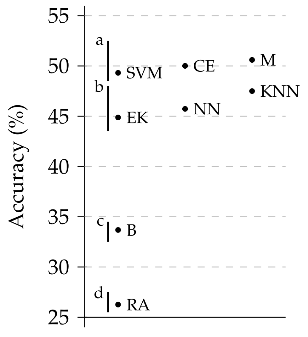
In order to validate the previous claims, a bootstrapping validation was used [51]. Thus, 100 samples were randomly built following the original distribution for the Silesia data sets. Figure 9 shows a box plot with the results of the different models bringing to light the significant differences among them. In fact, a Friedman test confirms this hypothesis (p-value ). In order to assess the differences among the different models, a post-hoc analysis has been made following the procedure described in [52]. This procedure clusters all methods with similar results and gives them the same letter. It should be taken into consideration that these groups are not sorted, namely, the best algorithms are not labeled with an a. The results are shown in Figure 10. In this figure, the mean value of the different algorithms is plotted and groups are identified with a letter. As can be seen, the test confirm our claims. The three groups are clearly visible.
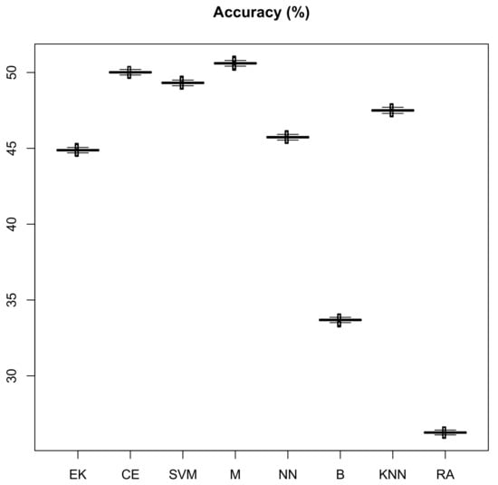
Figure 9.
Box plot of the distribution of the models’ accuracy of the three transport modes on 100 bootstrapping samples. In Biscay, the probability of using BICYCLE, CAR, MOTORCYCLE, TRANSIT, and WALK is 1.75%, 43.51%, 2.1%, 37.6%, and 15.04%, respectively. In Silesia, the probability of using BICYCLE, CAR, MOTORCYCLE, TRANSIT, and WALK is 0.82%, 53.96%, 0.12%, 36.33%, and 8.75%, respectively. Therefore, if a model can produce such a forecast, it will achieve an accuracy of 100 %. Source: own research generated from R Statistical Suite [50].
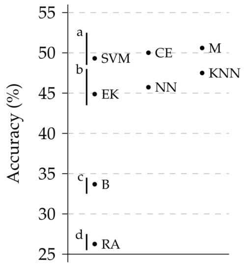
Figure 10.
Results of an ALL vs. ALL post-hoc analysis of the accuracy of the models. Source: own research by plotting the results from R Statistical Suite [50].
Again, when analyzing the results in detail, problems arise for some of the models. Looking at the confusion matrices (Table A2) highlights the fact that some models continue to have problems with some of the classes. For example, the SVM cannot correctly predict any WALK trip (even if it has correctly predicted half of the trips). The same problem occurs, when looking at the M and NN models, though it is not as acute. In the end, it seems that only the KNN, EK, and CE models do not suffer these problems in the setting.
Finally, Table 6 shows the forecasts that the different models share. As before, 100 bootstrapping samples were built from the Silesia data set. Column Real shows the results of the survey carried out in 2015 [26], and Columns L.C.I. and U.C.I. contain the lower and upper confidence interval at the 0.05 significant level () for the forecast value made. As expected, given the low variance of the bootstrapped samples (see Figure 9) the modal split forecasts of all models are quite similar (the confidence intervals are quite narrow). Nevertheless, the real value is not included in the confidence interval.

Table 6.
Bootstraping values (in %) for the modal split forecast by the different models. Source: own research.
4. Conclusions and Future Work
This article presents eight methodologies for building transport choice models according to FSM. The methodologies were trained for one scenario, Biscay (Basque Country, Spain), and later evaluated with a second scenario, Silesian Voivodeship (Poland). As explained in Section 3, the results suggest the existence of three groups of models: On the one hand, as expected, the most complex models tested (SVM, CE, and M) perform quite well, hitting almost half of the trips. Next, there is another set of complex algorithms but with slightly worse results (NN, EK, and KNN). The results of the KNN algorithm was in fact unexpected, as it is a very simple algorithm. On the other hand, the control methods (B and RA) do not achieve good results, as expected. In order to draw meaningful conclusions, a qualitative analysis should also be made:
- Some of the models produce unbalanced predictions, like M, SVM and NN, which completely ignore some of the transport modes. Therefore, given the similar prediction capabilities, the models with more balanced predictions should be used, namely, the EK, CE, and KNN models.
- The number of parameters and complexity of the models are not the same either. In this sense, simpler models should be preferred to more complex models. However, EK, CE, and KNN are non-parametric, and their complexity is difficult to assess. On the one hand, the number of parameters of KNN is indeed the amount of points in the training data set, but the complexity of the model is quite low (understanding here the complexity in terms of its VC dimension or similar measures [53]). On the other hand, the amount of parameters in the EK and CE models is quite low (compared to the number of parameters of KNN), but the complexity of the model is higher [54].
- Comparing the EK and CE fuzzy rule sets, both have similar amounts of rules (EK has 33 and CE has 30). However, the EK rules are only composed of one or two terms, which makes it easy to follow and modify, while the CE evolved rules usually have about 10 or more terms with a relation between them that is not very clear.
- It is always better to use a model that is easy to be understood than a data-driven model. Following this advice, EK and M should be preferred to the rest of the models.
Based on the above considerations, it is clear that the best model is EK, as it is possible to be understood, is easy to be extended so as to cover new transport policies, has a complexity that is similar to other models that produce similar numerical results, and its predictions are well balanced among the classes.
Even though the results are good, the models need to be improved. At the moment, the methodology does not take into account socio-economic variables, which are not present on the tested data sets (see Table 2). Recent works ([55,56]) have achieved successful results by using demographic and socio-economic features. As shown in [56] (where they have almost reached a 90% chance of success), socio-economic information from commuters enables the clustering and creation of custom utility functions for each group. Furthermore, climatic variables have been identified as relevant [28]. Future refinements of the model may introduce both sets of variables in search of reducing error. A first approach should consist of adding these non-trip related features to the global census models and evaluate their improvement. In case this is not satisfactory, the next step will be to try clustering the commuters and adjusting the models for each group.
Additionally, the ownership of private vehicles is a relevant parameter not detailed in the used data sets. In order to introduce this information, the model will use Monte Carlo simulations so that several distributions of these variables are simulated and the results assessed.
Finally, once the transport choice model is fitted, the next step is to determine the extent to which different non-physical incentives, such as changes in the price of the journey, discounts on public transport, additional taxes on the use of private vehicles, reductions in the duration of the journey, and congestion charges, affect commuters’ choices. These incentives alter the features of the itineraries, resulting in a different modal split. In order to check the suitability of these incentives, the citizen agents within the simulation will be given a set of preferences that will determine whether they are prone to accept or ignore a certain policy, based on the itinerary features already modeled in the transport choice model. This approach will involve defining the thresholds at which the applications of transport policies will be effective, all the while seeking an equilibrium between the objectives of the policies and the citizens’ preferences in order to avoid social rejection or oversizing.
Acknowledgments
This work was partially supported by (a) the GREENTRAVELLING project (Era NET Transport 6/12/IN/2014/195 label) partially funded by Diputación Foral de Bizkaia through the Plan de Promoción de la Innovación (6/12/-IN/2014/195) and the Basque Government through the GAITEK program IG-2014/0000133), (b) the S-MILE project (Era NET Transport ENTIII Flagship 2015 label) funded by Basque Government through the HAZITEK program (ZL-2017/00081), and (c) the Industrial Ph.D. grant given by the University of Deusto (2015–2018).
Author Contributions
Ander Pijoan, Oihane Kamara-Esteban, Ainhoa Alonso-Vicario and Cruz E. Borges. conceived and designed the experiments, performed the analysis of the results and contributed to the writing of the manuscript.
Conflicts of Interest
The authors declare no conflict of interest.
Appendix A. Result tables
Table A1.
Confusion matrices for all the models for the five transport modes (in %). Source: own research.

(a) Expert Knowledge Confusion Matrix
(a) Expert Knowledge Confusion Matrix
| Biscay | Silesia | ||||||||||
|---|---|---|---|---|---|---|---|---|---|---|---|
| Observed | Observed | ||||||||||
| B | C | M | T | W | B | C | M | T | W | ||
| Forecast | B | 20.9302 | 25.9588 | 13.5483 | 16.9042 | 22.9138 | 39.8180 | 6.3235 | 0 | 0.0005 | 0.0051 |
| C | 14.3410 | 19.8004 | 11.6129 | 18.5639 | 6.8561 | 3.597 | 23.9876 | 8.5339 | 5.12764 | 53.5860 | |
| M | 18.9922 | 14.4995 | 23.8709 | 21.0896 | 23.0491 | 13.3028 | 8.1699 | 20.8480 | 1.726741 | 12.15994 | |
| T | 12.7906 | 17.5709 | 14.8387 | 14.0898 | 4.2399 | 16.4029 | 12.1599 | 60.1307 | 24.0259 | 33.56175 | |
| W | 32.9457 | 22.1702 | 36.1290 | 29.3523 | 42.9409 | 26.8792 | 49.3589 | 10.4874 | 69.1292 | 0.6872 | |

(b) Co-evolutionary Fuzzy Algorithm Confusion Matrix
(b) Co-evolutionary Fuzzy Algorithm Confusion Matrix
| Biscay | Silesia | ||||||||||
|---|---|---|---|---|---|---|---|---|---|---|---|
| Observed | Observed | ||||||||||
| B | C | M | T | W | B | C | M | T | W | ||
| Forecast | B | 25.5814 | 18.45266 | 28.70968 | 22.90614 | 20.75812 | 4.3421 | 3.6566 | 3.2258 | 4.0652 | 5.2098 |
| C | 5.03876 | 26.15817 | 3.870968 | 5.018051 | 3.745487 | 43.2894 | 55.6609 | 20.9677 | 50.0042 | 14.4617 | |
| M | 0 | 0 | 0 | 0 | 0 | 46.3157 | 35.6888 | 64.5161 | 40.3782 | 48.2227 | |
| T | 24.03101 | 31.14959 | 24.51613 | 29.07942 | 5.685921 | 0.3947 | 0.1415 | 0 | 0.1385 | 0.5517 | |
| W | 45.34884 | 24.23959 | 42.90323 | 42.99639 | 69.81047 | 5.6578 | 4.8519 | 11.2903 | 5.4137 | 31.5539 | |

(c) Support Vector Machine Confusion Matrix
(c) Support Vector Machine Confusion Matrix
| Biscay | Silesia | ||||||||||
|---|---|---|---|---|---|---|---|---|---|---|---|
| Observed | Observed | ||||||||||
| B | C | M | T | W | B | C | M | T | W | ||
| Forecast | B | 0 | 0 | 0 | 0 | 0 | 0 | 0 | 0 | 0 | 0 |
| C | 34.1085 | 63.6576 | 36.7741 | 38.2283 | 11.1411 | 61.7693 | 68.9583 | 43.7908 | 65.7117 | 77.1642 | |
| M | 0 | 0 | 0 | 0 | 0 | 0 | 0 | 0 | 0 | 0 | |
| T | 65.8914 | 36.3423 | 63.2258 | 61.7716 | 88.8588 | 38.2306 | 31.0416 | 56.2091 | 34.2882 | 22.8357 | |
| W | 0 | 0 | 0 | 0 | 0 | 0 | 0 | 0 | 0 | 0 | |

(d) Multinomial Confusion Matrix
(d) Multinomial Confusion Matrix
| Biscay | Silesia | ||||||||||
|---|---|---|---|---|---|---|---|---|---|---|---|
| Observed | Observed | ||||||||||
| B | C | M | T | W | B | C | M | T | W | ||
| Forecast | B | 3.0076 | 0 | 0 | 0 | 0 | 0 | 0 | 0 | 0 | 0 |
| C | 34.2105 | 64.5774 | 118 | 2306 | 248 | 63.1384 | 71.4683 | 44.117 | 68.3363 | 15.8941 | |
| M | 0 | 0 | 0 | 0 | 0 | 0.1843 | 0.6491 | 0 | 0.5331 | 0.0051 | |
| T | 62.7819 | 35.3445 | 192 | 3236 | 1969 | 36.5718 | 27.8083 | 55.8823 | 31.0581 | 83.6567 | |
| W | 0 | 0.0779 | 0 | 1 | 0 | 0.1053 | 0.0742 | 0 | 0.0723 | 0.4439 | |

(e) Neural Network Confusion Matrix
(e) Neural Network Confusion Matrix
| Biscay | Silesia | ||||||||||
|---|---|---|---|---|---|---|---|---|---|---|---|
| Observed | Observed | ||||||||||
| B | C | M | T | W | B | C | M | T | W | ||
| Forecast | B | 0 | 0.0155 | 0 | 0 | 0 | 0.0263 | 0.0233 | 0 | 0.0316 | 0.0487 |
| C | 33.0827 | 63.5640 | 115 | 2250 | 298 | 42.7330 | 52.2078 | 26.1437 | 48.8802 | 17.4520 | |
| M | 0 | 0 | 0 | 0 | 0 | 0.1053 | 0.0623 | 0 | 0.0593 | 0.2540 | |
| T | 62.4060 | 36.0773 | 193 | 3257 | 1883 | 56.7667 | 47.2574 | 72.8758 | 50.5170 | 81.1723 | |
| W | 1.5037 | 0.3429 | 2 | 36 | 36 | 0.3686 | 0.4490 | 0.9803 | 0.5116 | 1.0727 | |

(f) Naïve Bayesian Confusion Matrix
(f) Naïve Bayesian Confusion Matrix
| Biscay | Silesia | ||||||||||
|---|---|---|---|---|---|---|---|---|---|---|---|
| Observed | Observed | ||||||||||
| B | C | M | T | W | B | C | M | T | W | ||
| Forecast | B | 3.3835 | 0.2806 | 0.3225 | 0.2164 | 0 | 0.9215 | 2.4044 | 1.6339 | 1.0844 | 0.8469 |
| C | 9.3984 | 29.7006 | 7.7419 | 7.4688 | 4.1948 | 26.5139 | 31.6341 | 17.9738 | 30.5481 | 17.5213 | |
| M | 0 | 0 | 0 | 0 | 0 | 0.7635 | 0.5622 | 0 | 0.6038 | 0.6980 | |
| T | 18.7969 | 27.2840 | 20.3225 | 26.3575 | 5.1420 | 18.6677 | 24.3470 | 7.8431 | 21.9218 | 0.1154 | |
| W | 68.4210 | 42.7346 | 71.6129 | 65.9570 | 90.6630 | 53.1332 | 41.0521 | 72.5490 | 45.8417 | 80.8181 | |

(g) k-Nearest Neighbours Confusion Matrix
(g) k-Nearest Neighbours Confusion Matrix
| Biscay | Silesia | ||||||||||
|---|---|---|---|---|---|---|---|---|---|---|---|
| Observed | Observed | ||||||||||
| B | C | M | T | W | B | C | M | T | W | ||
| Forecast | B | 0 | 0 | 0 | 0 | 0 | 0 | 0 | 0 | 0 | 0 |
| C | 33.4586 | 64.4839 | 37.0967 | 33.1048 | 21.2449 | 52.9489 | 61.7642 | 38.2352 | 58.5322 | 26.5013 | |
| M | 0 | 0 | 0 | 0 | 0 | 0 | 0 | 0 | 0 | 0 | |
| T | 54.1353 | 31.6027 | 54.8387 | 60.7793 | 60.9833 | 44.7077 | 36.1090 | 58.8235 | 39.1705 | 61.8109 | |
| W | 12.406 | 3.9133 | 8.0645 | 6.1158 | 17.7717 | 2.3433 | 2.1267 | 2.9411 | 2.2972 | 11.6877 | |

(h) Random Search Confusion Matrix
(h) Random Search Confusion Matrix
| Biscay | Silesia | ||||||||||
|---|---|---|---|---|---|---|---|---|---|---|---|
| Observed | Observed | ||||||||||
| B | C | M | T | W | B | C | M | T | W | ||
| Forecast | B | 0 | 0 | 0 | 0 | 0 | 0 | 0 | 0 | 0 | 0 |
| C | 100 | 100 | 100 | 100 | 100 | 0 | 0.1434 | 1.9608 | 5.1742 | 23.0056 | |
| M | 0 | 0 | 0 | 0 | 0 | 100 | 85.717 | 98.0392 | 91.1507 | 76.2244 | |
| T | 0 | 0 | 0 | 0 | 0 | 0 | 0 | 0 | 3.6751 | 0 | |
| W | 0 | 0 | 0 | 0 | 0 | 0 | 14.1396 | 0 | 0 | 0.7699 | |
Table A2.
Confusion matrices for all the models for the three transport modes (in %). Source: own research.

(a) Expert Knowledge Confusion Matrix
(a) Expert Knowledge Confusion Matrix
| Biscay | Silesia | ||||||
|---|---|---|---|---|---|---|---|
| Observed | Observed | ||||||
| P | T | W | P | T | W | ||
| Forecast | P | 27.2306 | 8.5771 | 10.8617 | 64.3052 | 60.4932 | 32.9044 |
| T | 47.6867 | 51.6633 | 27.5583 | 0.0528 | 0.0587 | 0.4739 | |
| W | 25.0826 | 39.7595 | 61.5798 | 35.6419 | 39.4479 | 66.6216 | |

(b) Co-evolutionary Confusion Matrix
(b) Co-evolutionary Confusion Matrix
| Biscay | Silesia | ||||||
|---|---|---|---|---|---|---|---|
| Observed | Observed | ||||||
| P | T | W | P | T | W | ||
| Forecast | P | 27.8851 | 6.9637 | 5.2929 | 23.3397 | 26.4874 | 15.1919 |
| T | 44.8245 | 46.1122 | 21.0505 | 40.5583 | 55.2673 | 59.8538 | |
| W | 27.2903 | 46.9240 | 73.6565 | 36.102 | 18.2453 | 24.9543 | |

(c) Suport Vector Machine Confusion Matrix
(c) Suport Vector Machine Confusion Matrix
| Biscay | Silesia | ||||||
|---|---|---|---|---|---|---|---|
| Observed | Observed | ||||||
| P | T | W | P | T | W | ||
| Forecast | P | 63.9797 | 40.0144 | 14.1414 | 63.9771 | 60.4658 | 20.4924 |
| T | 36.0202 | 59.9855 | 85.7373 | 36.0228 | 39.5341 | 79.5075 | |
| W | 0 | 0 | 0.1212 | 0 | 0 | 0 | |

(d) Multinomial Confusion Matrix
(d) Multinomial Confusion Matrix
| Biscay | Silesia | ||||||
|---|---|---|---|---|---|---|---|
| Observed | Observed | ||||||
| P | T | W | P | T | W | ||
| Forecast | P | 65.9131 | 44.1096 | 15.1919 | 76.5456 | 74.0214 | 22.5083 |
| T | 34.0124 | 55.8722 | 84.8080 | 23.3329 | 25.8451 | 77.0076 | |
| W | 0.0743 | 0.0180 | 0 | 0.1214 | 0.1334 | 0.4840 | |

(e) Neural Network Confusion Matrix
(e) Neural Network Confusion Matrix
| Biscay | Silesia | ||||||
|---|---|---|---|---|---|---|---|
| Observed | Observed | ||||||
| P | T | W | P | T | W | ||
| Forecast | P | 58.0011 | 36.3882 | 14.9090 | 47.2961 | 47.0370 | 24.9403 |
| T | 41.6121 | 63.1968 | 83.9595 | 51.6283 | 51.9418 | 70.7169 | |
| W | 0.3866 | 0.4149 | 1.1313 | 1.0754 | 1.0211 | 4.3426 | |

(f) Naïve Bayes Confusion Matrix
(f) Naïve Bayes Confusion Matrix
| Biscay | Silesia | ||||||
|---|---|---|---|---|---|---|---|
| Observed | Observed | ||||||
| P | T | W | P | T | W | ||
| Forecast | P | 28.9708 | 7.6853 | 4.8080 | 34.6062 | 32.2438 | 19.8774 |
| T | 26.9333 | 26.3575 | 6.6262 | 24.3029 | 21.9127 | 1.7585 | |
| W | 44.0957 | 65.9570 | 88.5656 | 41.0908 | 45.8434 | 78.3639 | |

(g) Random Search Confusion Matrix
(g) Random Search Confusion Matrix
| Biscay | Silesia | ||||||
|---|---|---|---|---|---|---|---|
| Observed | Observed | ||||||
| P | T | W | P | T | W | ||
| Forecast | P | 99.9366 | 99.9431 | 100 | 22.3468 | 100 | 100 |
| T | 0 | 0 | 0 | 77.6532 | 0 | 0 | |
| W | 0.0633 | 0.0568 | 0 | 0 | 0 | 0 | |

(h) K-Nearest Neighbours Confusion Matrix
(h) K-Nearest Neighbours Confusion Matrix
| Biscay | Silesia | ||||||
|---|---|---|---|---|---|---|---|
| Observed | Observed | ||||||
| P | T | W | P | T | W | ||
| Forecast | P | 65.9875 | 36.4604 | 25.3737 | 64.2006 | 61.2099 | 31.7244 |
| T | 29.0898 | 55.9985 | 53.4949 | 33.0386 | 35.7617 | 54.8664 | |
| W | 4.9226 | 7.5410 | 21.1313 | 2.7607 | 3.0282 | 13.4091 | |
References
- De Donnea, F.X. The Determinants of Transport Mode Choice in Dutch Cities: Some Disaggregate Stochastic Models; Universitaire Pers Rotterdam: Rotterdam, The Netherlands, 1971. [Google Scholar]
- Holtsmark, B.; Skonhoft, A. The Norwegian support and subsidy policy of electric cars. Should it be adopted by other countries? Environ. Sci. Policy 2014, 42, 160–168. [Google Scholar] [CrossRef]
- Karlaftis, M.G.; Vlahogianni, E.I. Statistical methods versus neural networks in transportation research: Differences, similarities and some insights. Transp. Res. Part C Emerg. Technol. 2011, 19, 387–399. [Google Scholar] [CrossRef]
- Fernández-Isabel, A.; Fuentes-Fernández, R. An agent-based platform for traffic simulation. In Soft Computing Models in Industrial and Environmental Applications, 6th International Conference SOCO 2011; Springer: Berlin/Heidelberg, Germany, 2011; pp. 505–514. [Google Scholar]
- Bazzan, A.L.; Klügl, F. A review on agent-based technology for traffic and transportation. Knowl. Eng. Rev. 2014, 29, 375–403. [Google Scholar] [CrossRef]
- Rubinstein, R.Y.; Kroese, D.P. Simulation and the Monte Carlo Method; John Wiley & Sons: Hoboken, NJ, USA, 2016; Volume 10. [Google Scholar]
- Keilson, J. Markov Chain Models—Rarity and Exponentiality; Springer Science & Business Media: Berlin, Germany, 2012; Volume 28. [Google Scholar]
- Allen, A.O. Probability, Statistics, and Queueing Theory; Academic Press: Cambridge, MA, USA, 2014. [Google Scholar]
- Meyer, M.D.; Miller, E.J. Urban Transportation Planning: A Decision-Oriented Approach; McGraw-Hill: New York, NY, USA, 1984. [Google Scholar]
- McNally, M.G. The four-step model. In Handbook of Transport Modelling, 2nd ed.; Emerald Group Publishing Limited: Bingley, UK, 2007; pp. 35–53. [Google Scholar]
- Wooldridge, M.; Jennings, N.R. Intelligent Agents: Theory and Practice; Cambridge University Press: Cambridge, UK, 1995. [Google Scholar]
- Owen, L.E.; Zhang, Y.; Rao, L.; McHale, G. Street and traffic simulation: Traffic flow simulation using CORSIM. In Proceedings of the 32nd conference on Winter simulation, Orlando, FL, USA, 10–13 December 2000; pp. 1143–1147. [Google Scholar]
- Saad, F. In-depth analysis of interactions between drivers and the road environment: Contribution of on-board observations and subsequent verbal report. In Proceedings of the 4th Workshop of ICTCT, University of Lund, Vienna, Austria, November 1992. [Google Scholar]
- PTV AG. PTV Vissim 7—USER MANUAL; PTV AG: Karlsruhe, Njemačka, 2015. [Google Scholar]
- Barceló, J.; Casas, J. Dynamic network simulation with AIMSUN. In Simulation Approaches in Transportation Analysis; Springer: Boston, MA, USA, 2005; pp. 57–98. [Google Scholar]
- Halati, A.; Lieu, H.; Walker, S. CORSIM-corridor traffic simulation model. In Proceedings of the Traffic Congestion and Traffic Safety in the 21st Century: Challenges, Innovations, and Opportunities, Chicago, IL, USA, 8–11 June 1997. [Google Scholar]
- Mahmassani, H. Dynamic traffic assignment and simulation for advanced network informatics (DYNASMART). In Proceedings of the 2nd International Seminar on Urban Traffic Networks, Capri, Italy, 5–8 July 1992. [Google Scholar]
- Smith, L.; Beckman, R.; Anson, D.; Nagel, K.; Williams, M. TRANSIMS: Transportation Analysis and Simulation System; Technical Report; Los Alamos National Lab.: Los Alamos, NM, USA, 1995.
- Babin, A.; Florian, M.; James-Lefebvre, L.; Spiess, H. Emme/2 an interactive graphic method for road and transit planning. In Proceedings of the RTAC Annual Conference Preprints, Washington, DC, USA, 18–22 January 1981; Volume 1. [Google Scholar]
- PTV Group Ptv Visum. 2016. Available online: http://your.visum.ptvgroup.com/FreeDemoVersion (accessed on 4 November 2016).
- Ji, M.; Yu-long, P. Development and application of TransCAD for urban traffic planning. J. Harbin Univ. Civ. Eng. Archit. 2002, 5, 028. [Google Scholar]
- Balcombe, R.; Mackett, R.; Paulley, N.; Preston, J.; Shires, J.; Titheridge, H.; Wardman, M.; White, P. The Demand for Public Transport: A Practical Guide; Transportation Research Laboratory: Wokingham, UK, 2004. [Google Scholar]
- Train, K. Qualitative Choice Analysis: Theory, Econometrics, and an Application to Automobile Demand, 1st ed.; The MIT Press: Cambridge, MA, USA, 1985; Volume 1. [Google Scholar]
- Rich, J.; Holmblad, P.; Hansen, C. A weighted logit freight mode-choice model. Transp. Res. Part E Logist. Transp. Rev. 2009, 45, 1006–1019. [Google Scholar] [CrossRef]
- Instituto Nacional de Estadística. Censos 2011. 2011. Available online: http://www.ine.es/censos2011_datos/cen11_datos_resultados.html (accessed on 13 April 2018).
- Green Travelling Consortium. A Platform to Analyse and Foster the Use of Green Travelling Options; Technical Report, Project Proposal, The ERA-NET Transport III: Future Travelling; Avda. Universidades: Bilbao, Spain, 2013. [Google Scholar]
- Domencich, T.A.; McFadden, D. Urban Travel Demand—A Behavioral Analysis; North-Holland Publishing Co.: Amsterdam, The Netherlands, 1975. [Google Scholar]
- Chiu Chuen, O.; Karim, M.R.; Yusoff, S. Mode Choice between Private and Public Transport in Klang Valley, Malaysia. Sci. World J. 2014, 2014, 394587. [Google Scholar] [CrossRef] [PubMed]
- Clauss, T.; Döppe, S. Why do urban travelers select multimodal travel options: A repertory grid analysis. Transp. Res. Part A Policy Pract. 2016, 93, 93–116. [Google Scholar] [CrossRef]
- Pijoan, A.; Borges, C.E.; Oribe-Garcia, I.; Martin, C.; Alonso-Vicario, A. Agent Based Simulations for the Estimation of Sustainability Indicators. Procedia Comput. Sci. 2015, 51, 2943–2947. [Google Scholar] [CrossRef]
- Altman, N.S. An introduction to kernel and nearest-neighbor nonparametric regression. Am. Stat. 1992, 46, 175–185. [Google Scholar]
- Lemeshow, S.; Sturdivant, R.X.; Hosmer, D.W. Applied Logistic Regression; Wiley: Hoboken, NJ, USA, 2013. [Google Scholar]
- Cristianini, N.; Shawe-Taylor, J. An Introduction to Support Vector Machines and Other Kernel-Based Learning Methods; Cambridge University Press: Cambridge, UK, 2000. [Google Scholar]
- Schalkoff, R.J. Artificial Neural Networks; McGraw-Hill: New York, NY, USA, 1997; Volume 1. [Google Scholar]
- Lewis, D.D. Naive (Bayes) at forty: The independence assumption in information retrieval. In Machine Learning: ECML-98; Springer: Berlin/Heidelberg, Germany, 1998; pp. 4–15. [Google Scholar]
- Mendel, J.M. Uncertain Rule-Based Fuzzy Logic Systems: Introduction and New Directions; Prentice Hall PTR: Upper Saddle River, NJ, USA, 2001. [Google Scholar]
- Souche, S. Measuring the structural determinants of urban travel demand. Transp. Policy 2010, 17, 127–134. [Google Scholar] [CrossRef]
- Chang, C.C.; Lin, C.J. LIBSVM: A Library for Support Vector Machines. ACM Trans. Intell. Syst. Technol. 2011, 2, 27:1–27:27. [Google Scholar] [CrossRef]
- Von Seggern, D.H. CRC Standard Curves and Surfaces with Mathematica; CRC Press: Boca Raton, FL, USA, 2006. [Google Scholar]
- Kumar, M.; Sarkar, P.; Madhu, E. Development of fuzzy logic based mode choice model considering various public transport policy options. Int. J. Traffic Transp. Eng. 2013, 3, 408–425. [Google Scholar] [CrossRef]
- Tuzkaya, U.R.; Önüt, S. A fuzzy analytic network process based approach to transportation-mode selection between Turkey and Germany: A case study. Inf. Sci. 2008, 178, 3133–3146. [Google Scholar] [CrossRef]
- Berkan, R.C.; Trubatch, S. Fuzzy System Design Principles; Wiley-IEEE Press: Hoboken, NJ, USA, 1997. [Google Scholar]
- Staniek, M.; Sierpiński, G. Cost Criteria as a Means to Support Travelling Mode Related Decisions—A Case Study for the Central Part of Silesian Voivodeship (Poland). In Sustainable Transport Development, Innovation and Technology; Springer: Cham, Switzerland, 2016; pp. 137–150. [Google Scholar]
- Sierpiński, G.; Staniek, M.; Celiński, I. Travel behavior profiling using a trip planner. Transp. Res. Procedia 2016, 14, 1743–1752. [Google Scholar] [CrossRef]
- Herrera, F. Genetic fuzzy systems: Taxonomy, current research trends and prospects. Evolut. Intell. 2008, 1, 27–46. [Google Scholar] [CrossRef]
- Potter, M.A.; De Jong, K.A. A cooperative coevolutionary approach to function optimization. In Parallel Problem Solving from Nature; Springer: Berlin/Heidelberg, Germany, 1994; pp. 249–257. [Google Scholar]
- Pijoan, A.; Kamara-Esteban, O.; Borges, C.E. Environment modelling for spatial load forecasting. In Agent Environments for Multi-Agent Systems IV; Springer: Verlag, New York, 2014; pp. 188–206. [Google Scholar]
- Rada-Vilela, J. Fuzzylite: A Fuzzy Logic Control Library. 2017. Available online: https://www.fuzzylite.com/ (accessed on 13 April 2018).
- Kuhn, M. caret: Classification and Regression Training; R Package Version 6.0-78; ASCL: Leicester, UK, 2017. [Google Scholar]
- R Core Team. R: A Language and Environment for Statistical Computing; R Foundation for Statistical Computing: Vienna, Austria, 2017. [Google Scholar]
- Efron, B. Bootstrap Methods: Another Look at the Jackknife. Ann. Stat. 1979, 7, 1–26. [Google Scholar] [CrossRef]
- Piepho, H.P. An Algorithm for a Letter-Based Representation of All-Pairwise Comparisons. J. Comput. Graph. Stat. 2004, 13, 456–466. [Google Scholar] [CrossRef]
- Vapnik, V.N.; Chervonenkis, A.Y. On the Uniform Convergence of Relative Frequencies of Events to Their Probabilities. Theory Probab. Appl. 1971, 16, 264–280. [Google Scholar] [CrossRef]
- Chen, Y.; Wang, J.Z. Support vector learning for fuzzy rule-based classification systems. IEEE Trans. Fuzzy Syst. 2003, 11, 716–728. [Google Scholar] [CrossRef]
- Khattak, Z.H.; Magalotti, M.J.; Miller, J.S.; Fontaine, M.D. Using New Mode Choice Model Nesting Structures to Address Emerging Policy Questions: A Case Study of the Pittsburgh Central Business District. Sustainability 2017, 9, 2120. [Google Scholar] [CrossRef]
- Ding, L.; Zhang, N. A travel mode choice model using individual grouping based on cluster analysis. Procedia Eng. 2016, 137, 786–795. [Google Scholar] [CrossRef]
© 2018 by the authors. Licensee MDPI, Basel, Switzerland. This article is an open access article distributed under the terms and conditions of the Creative Commons Attribution (CC BY) license (http://creativecommons.org/licenses/by/4.0/).

