Empirical Study of How Traffic Intensity Detector Parameters Influence Dynamic Street Lighting Energy Consumption: A Case Study in Krakow, Poland

Abstract

The deployment of dynamic street lighting, which adjusts lighting levels to fulfill particular needs, leads to energy savings. These savings contribute to the overall lighting infrastructure maintenance cost. Yet another contribution is the cost of traffic intensity data. The data is read directly from sensor systems or intelligent transportation systems (ITSs). The more frequent the readings are, the more costly they become, because of hardware capabilities, data transfer and software license costs, among others. The paper investigates a relationship between the frequency of readings, in particular the averaging window size and step, and achieved energy savings. It is based on a simulation, taking into account a representative part of a city and traffic intensity data, which span over a period of one year. While the energy consumption reduction is simulated, all data, including each luminaire power setting, induction loop locations and street characteristics, come from a representative sample of the city of Krakow, Poland. Controlling the power settings complies with the lighting standard CEN/TR 13201. Analysis of the outcomes indicates that the shorter the window size or step are, the more energy saving that is available. In particular, for the previous standard CEN/TR 13201 2004, having the window size and step at 15 min results in 26.75% of energy saving, while reducing these values to 6 min provides 27%. Savings are more profound for the current standard (CEN/TR 13201 2014), assuming a 15 min size and step results in 47.43%, while having a 6 min size and step provides 47.69%. The results can serve as a guideline for identifying the economic viability of dynamic lighting control systems. Additionally, it can be observed that the current lighting standard provides far greater potential for dynamic control then the previous standard.

1. Introduction

One of the main targets of the smart city concept is to improve quality of life. Among others it is provided through increased safety and sustainability. There are multiple domains these can be applied to, which are office and residential buildings, energy grids, natural resources, transport, mobility and logistics [1]. Street lighting is one of such domains. If appropriately deployed, it increases safety by delivering proper lighting where and when needed. It benefits both motorized citizens and pedestrians. On the other hand, proper lighting optimization, which regards pole and fixture placement, fixture selection and dynamic lighting control, leads to a significant power consumption reduction, enabling sustainability [2].

Outdoor lighting, and specifically street and road lights, play a significant role in increasing safety, as was mentioned above. However, economic aspects are also extremely important. Even a small energy saving, a single watt, at the luminaire level, contributes significantly to the operational cost, because of the effect of scale. It is estimated that a city with a population of 1 million has approximately 80,000 light points, which consume from 20 to 50 GWh per year, in Poland. A relationship between the population density and the number of light points in urbanized areas has been established experimentally—it is 8 light points per 100 citizens for Poland. It is based on the assumption that the wattage of a single luminaire varies from 60 to 150 on average.

There are also other effects such as light pollution, which is closely tied with well-being. Non-economic aspects of outdoor lighting and their analysis is out of the scope of this paper; however they are important side effects of both optimized design and dynamic control, which deliver as much light as needed and exactly where and when needed.

Dynamic outdoor lighting control also reduces lighting infrastructure operational costs. This is due to adjusting lighting levels to actual traffic conditions, weather, and so on, which results in energy saving [3,4]. In general, the less traffic, the dimmer the light points could be. On the other hand, acquiring access to traffic intensity data comes with some cost. It depends on capabilities of the traffic intensity detectors and their control systems, traffic control system software licensing, data transmission, processing and storage costs. In general, increasing the traffic intensity measurement frequency increases the operational cost. Thus finding a balance between energy savings and the sensor infrastructure cost is a key task for the successful deployment of economically viable outdoor lighting control.

The paper proposes guidelines that help with answering the question of whether dynamic control, taking into account traffic intensity, would reduce its cost of use. In particular this cost is influenced by traffic intensity data source parameters. Because the required information is a number of vehicles per time unit, the parameters of such readings are how often traffic intensity has to be read from the sensors, and what the time window size in which the measurements are accumulated is. As a result of multivariant photometric calculations and precise traffic intensity measurements, dependencies between the above two parameters and the energy saving are put forward. Knowing the energy savings, one can identify the most economically viable traffic intensity detector infrastructure.

It needs to be pointed out that outdoor lighting remote control also comes with some cost. However, it is often balanced by benefits such as reduced maintenance cost. This is due to precise information regarding luminaire health, including failure detection and failure prediction, as well as turning it remotely on and off, which makes additional controllers unnecessary, lowering infrastructure cost. The direct cost of the deployment and maintenance of such control systems is not the subject of this paper. It is due to its significant variability and high margins of both luminaire and control system manufacturers. The actual cost varies from deployment to deployment.

To summarize, the main goal of this paper is to verify a relationship between energy saving due to dynamic control of street lighting and traffic intensity data source parameters (how often data is read and how long the period over which it is accumulated is). Knowing the relationship gives guidelines towards the economic viability of the dynamic control. The analysis is performed for the current lighting standard CEN/TR 13201, as well as for the previous standard, to identify possible energy-saving-related differences and make them applicable to existing and future deployments. It is based on a representative example of street lighting installation and traffic intensity detection in highly urbanized area of Krakow, Poland.

2. Related Research

Smart city and smart environment concepts and technologies are becoming part of everyday life. A growing number of available data sources providing information about our environment is one of the main reasons behind this. Data comes from standalone sensor systems and Internet-of-Things (IoT) devices [5,6,7]. Some of the main drivers are safety, quality of life and sustainability, including electric energy savings [2,8]. The smart city concepts can be applied at different scales. These could be the indoor or block scale [9,10], city scale, or regional scale [11]. Depending on the scale, a different type, amount and quality of sensor data is needed. We take a look at presence detection. At a building level, or at the general indoor scale, it is implemented as motion sensors with high spatial density. At the city level, such a detection is performed by motion or pressure sensors in the sidewalks and traffic intensity sensors in the streets—most commonly induction loops—with their spatial density decreased. At the regional level, it is mostly sparse traffic detection at highway entrances and exits—commonly with induction loops.

Street lighting is a representative example of applying smart city concepts, increasing safety and sustainability by adjusting lighting levels to particular needs [2,3,8]. Depending on the light source technology, control availability and actual area under consideration, being either highways or urban areas, different levels of energy consumption reduction can be achieved. Safety is guaranteed by complying with lighting norms and regulations [4].

It needs to be pointed out that one of the key enablers to dynamically adjust lighting levels is the light source technology shift. It replaces high-pressure sodium (HPS) sources with LEDs. LEDs are more energy efficient, but what is more important in this case is that their life span is not reduced by the act of dimming. Furthermore, it was confirmed that the energy consumption of the luminaires, which were subject to the experiments, depends almost linearly on the luminous flux, which cannot be said about HPS [3].

3. Dynamic Control Concept

The safety and convenience of outdoor lighting are precisely defined by the lighting standards, such as CEN/TR 13201 [12]. They define a notion of a lighting class. For a given street, a lighting class has to be selected on the basis of parameters such as the design speed or speed limit, traffic volume, traffic composition, separation of carriageway, junction density, presence of parked vehicles, ambient luminosity, navigational task difficulty, and so on. The class precisely defines lighting requirements that need to be met, such as light intensity and uniformity. To provide street lighting, for a given class at a given street, precise photometric calculations have to be performed in order to identify particular luminaire parameters, such as its type, power level, position on the pole, overhang, and so on, which are also subject to optimization [13].

The dynamic control selects the class, on the basis of data from sensors identifying varying environmental parameters such as traffic intensity. Changing the lighting class is possible as a result of Piéron’s law. The law describes a psychophysical regularity regarding signal detection. In particular, it states that mean response times (MRTs) decrease proportionally to a power of the stimulus intensity. Originally, the law was coined on the basis of observations of detection tasks in which the MRT was inverse to the stimulus luminance. A higher traffic intensity requires a shorter MRT, which could be achieved by increasing the light intensity [14]. If the traffic intensity drops below a certain threshold defined by the lighting standard, a lower lighting class can be selected, which results in less light and reduced energy consumption. Other class selection parameters, such as ambient light, weather conditions, and so on, could also be taken into consideration.

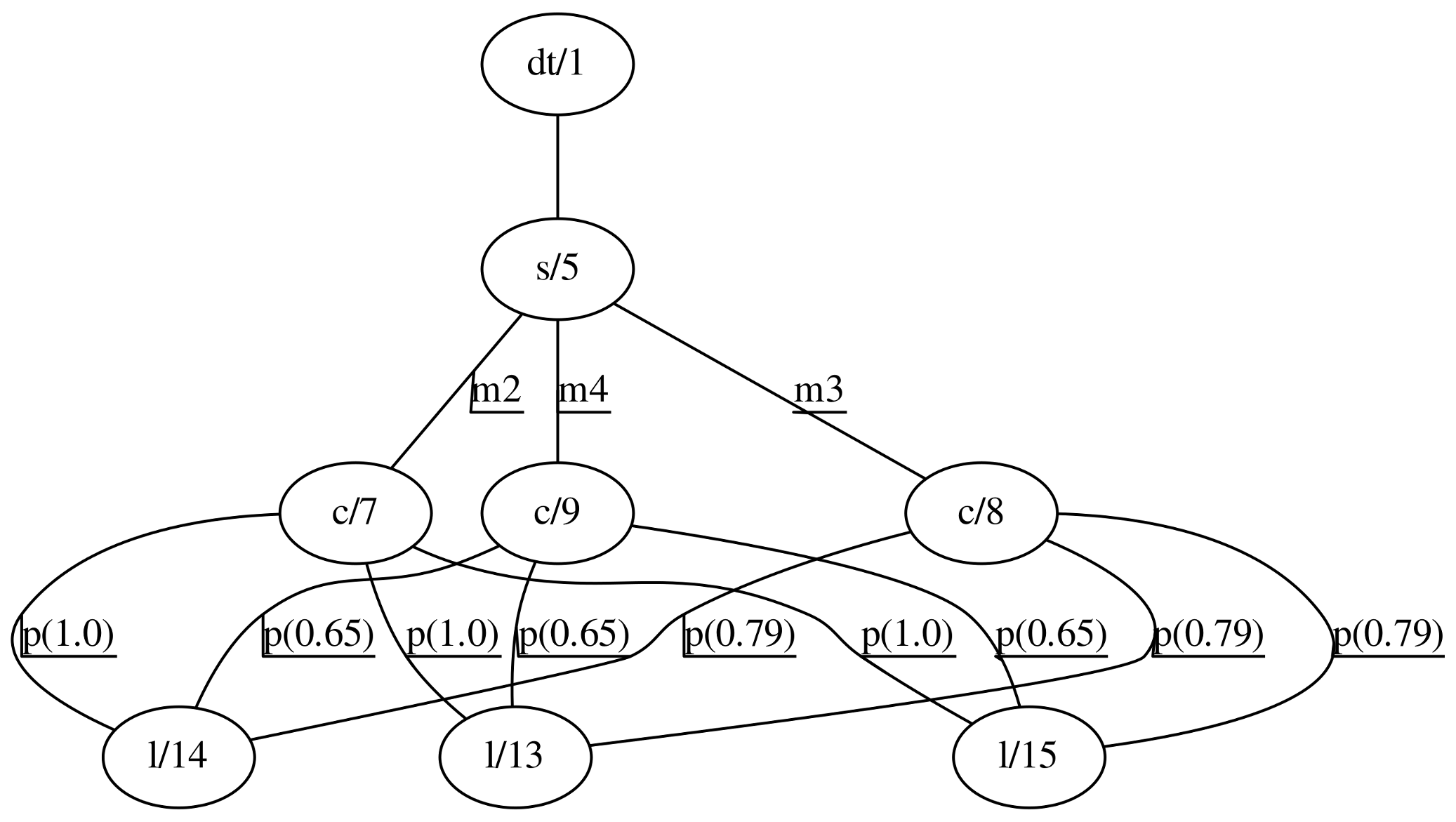
Furthermore, the dynamic control applies particular power settings for each of the luminaires to meet a given lighting class on a given street. Thus, it needs a formal model binding the above. An example of such a model is given in Figure 1 in the form of a control availability graph [4]. The proposed model utilizes a notion of segments. A segment is a uniform length of a street with all physical parameters being constant—for example, the same width, number of lanes, presence of sidewalks or median, and so on. A segment corresponds to a lighting situation in terms of the CEN/TR 13201 standard. The model is given as an undirected, labeled and attributed graph. Significant labels are shown at the corresponding vertices and edges. Optional vertex indices are preceded with “/”. For example, “s/5” stands for a vertex labeled with “s” and with an index of “5”, while “m2” indicates just a label. The meanings of the labels are as follows: “dt”: traffic intensity detector; “s”: street segment; “m2”, “m3” and “m4”: lighting classes; “c”: luminaire configuration; “l”: luminaire. The example graph models an environment with a single traffic intensity detector (“dt/1”) which delivers information about traffic intensity in the segment “s/5”. The segment has three configurations calculated: “c/7”, “c/8” and “c/9”, which if applied result in having “m2”, “m3” or “m4” lighting classes met. Each of the configurations holds particular power levels of the luminaires “l/13”, “l/14” and “l/15”, expressed as attributes and denoted as “name(value)”. For example, an edge between “c/7” and “l/14” is attributed “p(1.0)”, which indicates that upon selecting the configuration “c/7”, the power of luminaire “l/14” has to be set to “1.0”, which translates to 100% of the nominal power. Particular power levels are precalculated by photometric calculations, in accordance with the CEN/TR 13201 standard, which take into account the influence of the neighboring luminaires [15]. While the introduced graph regards a single detector (“dt”), the model is capable of processing not only traffic intensity information, but also ambient light levels (ambient luminosity), the presence of parked vehicles or speed limits (if it varies). The validity of other parameters such as weather conditions are still being researched. Thus, a single segment can have more detectors of diverse types. The model is compliant both with the CEN/TR 13201 2004 [16] and 2014 [12] standards. Any combination of parameter values and thresholds can be utilized in order to establish a proper lighting class according to the rules defined by the standards. The class selection depends on the data from sensors. Particular luminaire power settings are precalculated by performing photometric calculations and storing their results in the model. Having the proposed model ensures that the lighting always complies with the standards.

Furthermore, the model can be easily deployed in new locations, just by introducing topological relationships among segments, detectors and luminaires. For comparison, such new deployments with other smart lighting control solutions [17,18,19] are usually challenging—each deployment needs to be analyzed case by case and appropriately configured, which takes time and is costly.

4. Calculating Traffic Intensity

According to the lighting standard CEN/TR 13201, one of the factors that influences the selection of the lighting class, and thus the light intensity level, is the average traffic intensity. This is true both for an older version [16] and the current version [12]. The traffic intensity is expressed as the number of vehicles per day. However, the norm gives liberty regarding the method of how the actual traffic intensity is to be calculated. For the dynamic control, there is a need to have the traffic intensity calculated over a recent period of time. Answering the questions of “how recently” and “how often” the traffic intensity should be read influences the behavior of the control system, making it more or less responsive, and more or less economically viable. The more often the readings are taken, the more responsive the system is. The longer the time over which the readings are accumulated, the smoother the transitions between lighting classes are, which hypothetically can lead to less energy savings. More insights are given below.

In general, the more often the sensors deliver data, the more expensive it becomes. There are three main total cost components. First is the sensor system cost. The more capable detectors are, in terms of measurement frequency, the more expensive they become. Second is the communication cost. At some point all the measurements have to be transmitted either by hard lines or GPRS, which involves maintenance and transmission fees. Third is data processing and storage. The more data we have the more expensive its storage and processing are. The effect of scale is also there. A medium-size city is expected to have several thousands of traffic intensity detectors. Thus, they can generate massive amounts of data to be collected, transmitted and processed.

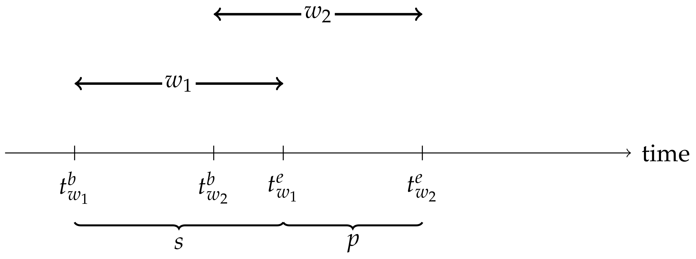
The traffic intensity is measured over a period of time with some frequency, which follows the moving averaging window concept. This is a time window in which traffic intensity is accumulated. There are two parameters of the window: the size s and the time step p. The time step indicates how often the data is delivered to the third parties, in this case, the dynamic lighting control system. The window size defines the period over which the vehicle count is accumulated. Utilizing the window applies a low-pass filter over the measurements. The greater the window size, the lower the frequency, or in other words, the smoother the characteristics become. An example visualizing such a window is given in Figure 2. For a moving window $w_n$ at the time $t_{w_n}^e$, there is a traffic intensity reading that takes into account traffic accumulated over a period of time from $t_{w_n}^b$ to $t_{w_n}^e$. The window size s is defined as

$$s=t_{w_n}^e-t_{w_n}^b=const,$$

while the step p is

$$p=t_{w_{n+1}}^e-t_{w_n}^e=const.$$

It needs to be pointed out that traffic intensity aggregation with short window sizes, which are comparable to the traffic light’s cycle time, is not reliable. They are subject to traffic intensity fluctuations due to traffic jams. Having a jam for 1.5 min results in counting zero vehicles moving within this period. However it does not mean that there is no traffic at all. Especially taking into account drivers’ anxiety [20], dimming lights on this account at the very moment could significantly impact safety. The traffic lights’ cycle time varies from intersection to intersection and from country to country [21,22]. Typical values range from 60 to 120 s. Thus, the window step should be significantly greater than the cycle time, or the window size should be long enough to compensate.

There are many sensor systems that deliver traffic intensity data, available both as an integral part of traffic lights (e.g., offered by Siemens) or standalone (e.g., offered by Kapsch). They can be standalone or part of an ITS. There are also third parties that deliver such data, for example, TomTom (both free and commercial licensing schemas), acting as providers. The data delivery frequency varies from 1 min to 1 h. A common value is a 15 min interval [5,19].

From the CEN/TR 13201 2004 [16] lighting standard perspective and possible lighting class change, the following traffic intensity values, expressed in vehicles per 24 h, are considered as thresholds: 7000, 15,000 and 25,000. If the traffic intensity crosses the threshold, it gives a basis for a lighting class change, which leads to dimming some luminaires, setting them to lower power. The 2014 standard [12] formally introduces adaptive control. It provides a notion of the normal class, which defines lighting conditions with the maximum value of average luminance or illuminance at any period of operation. Such a class can be lowered if the traffic volume drops below a certain percentage of the maximum capacity for a given point or uniform segment of a lane or carriageway.

As a result, it is expected to obtain power consumption characteristics on the basis of the window size and step. This would deliver a guideline for finding a balance between the sensor system costs and benefits from the energy savings.

The following sections regard

• the presentation of the representative test case in terms of luminaires, segments, lighting classes and traffic volume sensor availability,
• showing motivation for dynamic control on the basis of actual traffic intensity,
• an explanation for why both the current CEN/TR 13201 standard and the previous standard are taken into consideration,
• presenting energy savings for different moving window sizes and steps, and
• a discussion of the outcomes.

5. Representative Test Case

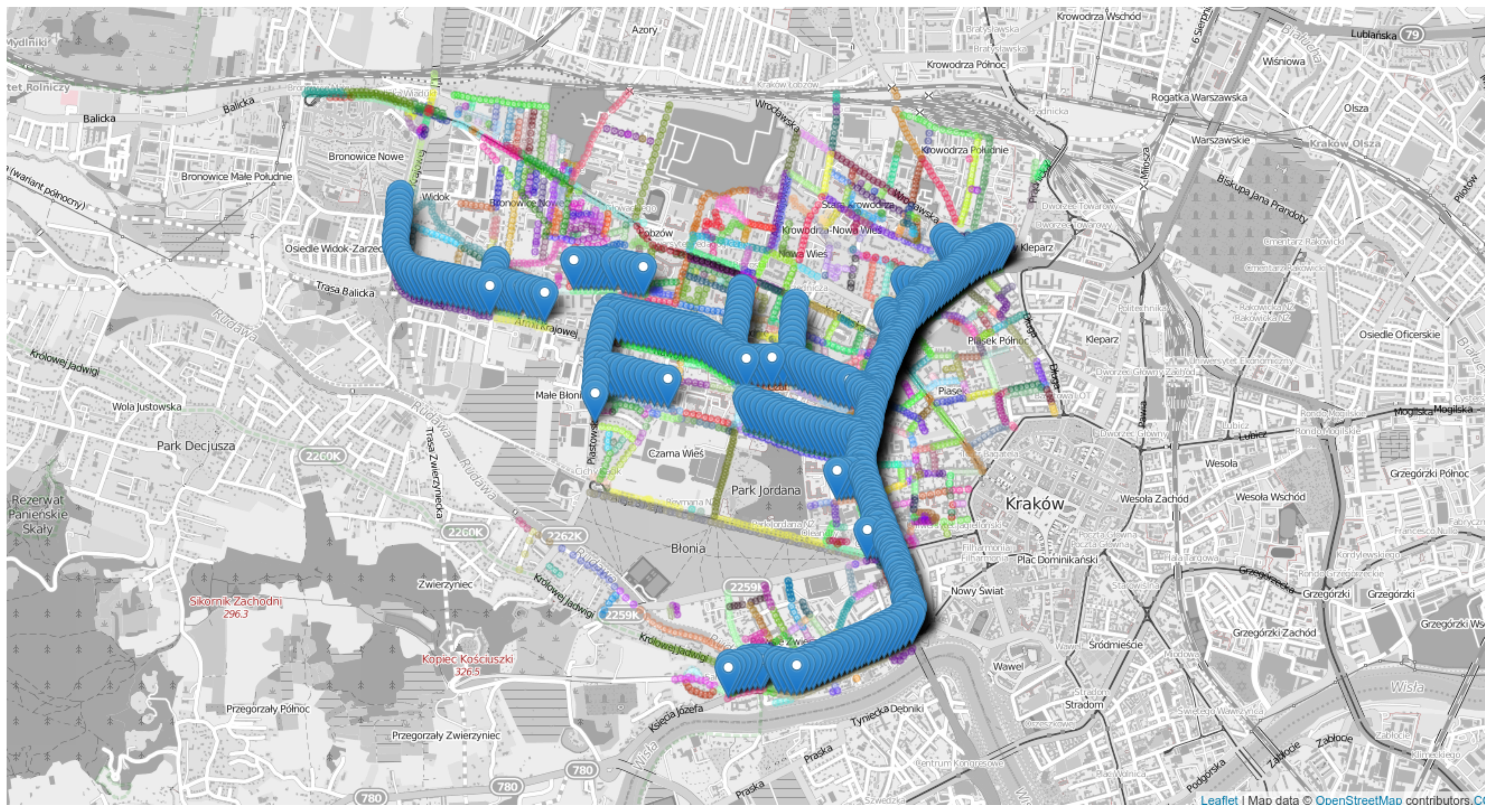
The test case regards a highly urbanized area, which is a part of the city of Krakow, one of the largest cities in Poland; see Figure 3. There were 324 remotely controlled fixtures with a cumulative power of 35.3 kW. They were clustered as 42 distinctive segments for which the traffic intensity was measured with induction loops (traffic intensity detectors).

There were 107 loops. Only the loops that measured traffic intensity in a particular segment were taken into consideration. No traffic flow in neighboring segments that did not have traffic intensity detectors was considered for this analysis. The traffic was measured over a period of every 1.5 min, which delivered raw data. On top of that, different window steps and sizes were simulated. A years’ worth of data ranges from 2015-06-23 to 2016-06-22.

The case took into consideration both CEN/TR 13201 2004 and 2014 standards regarding lighting class identification, photometric calculations and traffic-volume-based lighting class switching. This was to provide the aforementioned guideline for finding a balance between the sensor system cost and benefits from the energy savings for both the existing and future deployments. Therefore, the majority of existing deployments complied with the 2004 standard, while the new deployments should comply with the 2014 standard, considering both standards seem to be well justified. Thus, the simulation was run twice: once for the 2004 and once for 2014 standard—with appropriately adjusted control rules and the control availability graph to remain standard compliant.

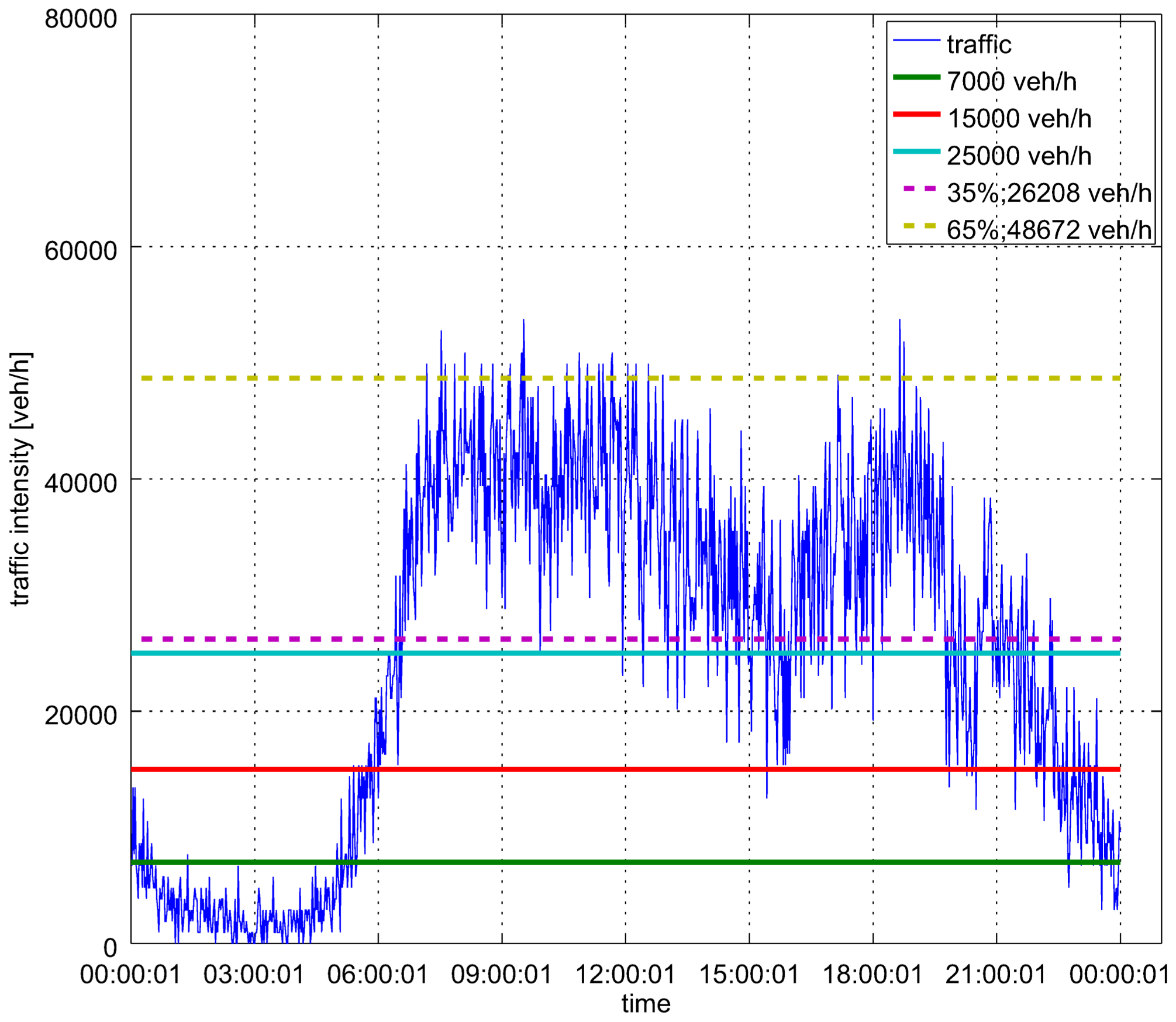
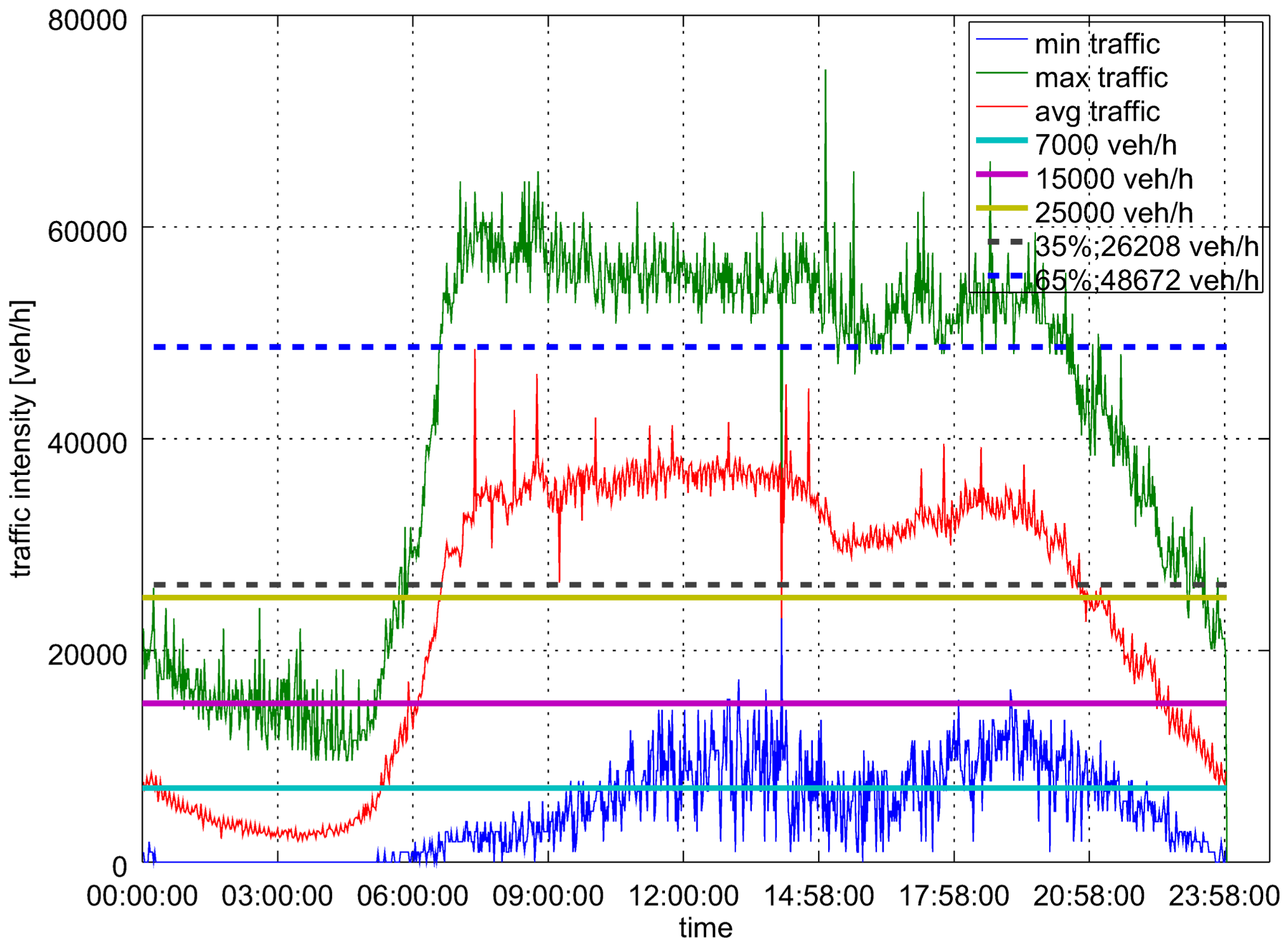
The daily traffic volume variability is shown in Figure 4 to present a rationale for lighting class switching. There are 7000, 15,000 and 25,000 vehicles per 24 h marks superimposed on the plot, which indicate possible lighting class changes according to the 2004 standard [16]. Marks for the 2014 standard [12] are shown as dashed lines. They are expressed as 35% and 65% of the maximum capacity of the multilane road in this case. If the traffic intensity crosses these marks, according to CEN/TR 13201, it enables lighting class switching, which results in dimming the luminaires, and in turn reducing energy usage.

Traffic intensity significantly varies on a day to day basis, which gives a motivation for dynamic control. Figure 5 shows these fluctuations indicating maximum, minimum and average traffic distributions over a 24 h period, taking into account a years’ worth of data. The 7000, 15,000 and 25,000 vehicles per 24 h marks together with the 35% and 65% marks are also superimposed.

The test case is a representative sample of a diverse street network. Details regarding lighting classes, the number of luminaires and the installed power are given in

Table 1. Base lighting classes for the test case, CEN/TR 13201 2004.

Class	Reduced Class	Luminaires (%)	Installed Power (%)
me2	me3b, me4a	65	76
me3c	me4b	30	19
me4b	me5	5	5

and

Table 2. Base lighting classes for the test case, CEN/TR 13201 2014.

Class	Reduced Class	Luminaires (%)	Installed Power (%)
m2	m3, m4	65	76
m3	m4, m5	30	19
m4	m5, m6	5	5

for the 2004 and 2014 standards, respectively. For the the 2004 standard, there were three base classes: “me2”, “me3c” and “me4b”, which could be lowered if the traffic intensity was reduced. Street classification resulted in the lighting situation set A3 being used with “me2” being assigned, which was switched at 25,000 or 15,000 vehicles per 24 h; B1 with “me3c” or “me4b” switched at 7000; and B2 with “me3c” switched at 7000. There were six lighting classes considered in total: “me2”, “me3c”, “me3b”, “me4b”, “me4a” and “me5”. For the the 2014 standard, there were three normal lighting classes: “m2”, “m3” and “m4”. Street classification resulted in “m2” being assigned to multilane routes. It could be switched to lower classes when the traffic volume was at 65% or 35% of the maximum capacity. The “m3” and “m4” were assigned to two lane routes for which switching could take place at 45% and 15%. There were a total of five classes being considered: “m2”, “m3”, “m4”, “m5” and “m6”.

We calculate the reference energy usage for the CEN/TR 13201 2004 standard. This is the total energy consumption on the basis of astronomical clock control. It assumes that the lights are turned on at sunset and that they are turned off at sunrise. It translates to 4,292.27 h/year, and 143,191,110 Wh consumed.

Applying a typical window size and step equal to 15 min, in which traffic is aggregated, and a years’ worth of traffic intensity readings regarding the test case area leads to energy consumption at 104,882,218 Wh. It yields 26.75% of energy savings compared with the reference.

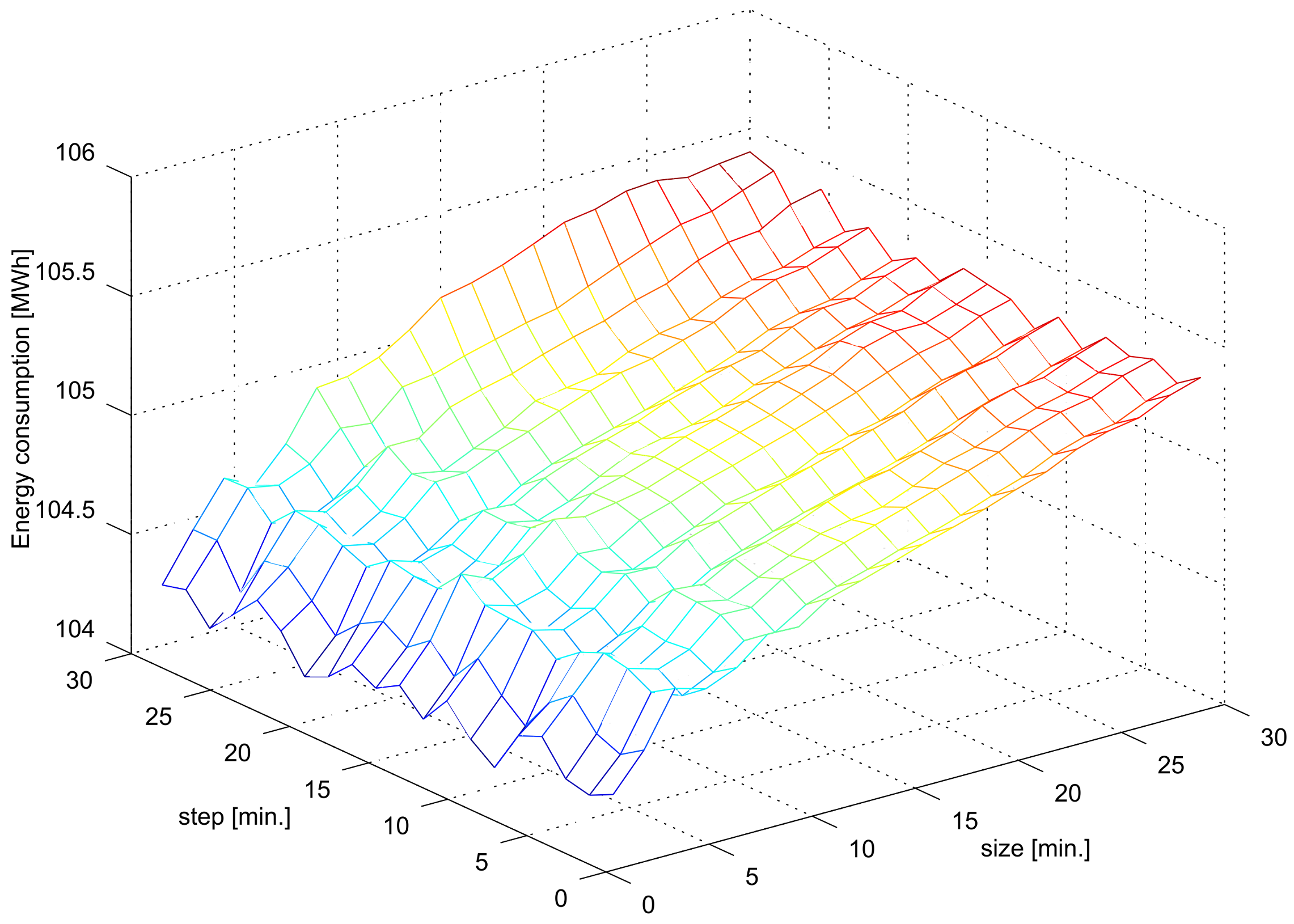
Adjusting the window size and step can provide better results. A comparison of different moving window sizes and steps’ overview is given in Figure 6. If the window step is greater than its size, then some traffic data is not taken into consideration. This could cause both over- or under-estimation, depending on whether the traffic was more or less intense in the missing period. It could make a particular street’s lighting invalid because of wrongly calculated traffic intensity. Hence, only cases with a size greater than or equal to the step should be considered. 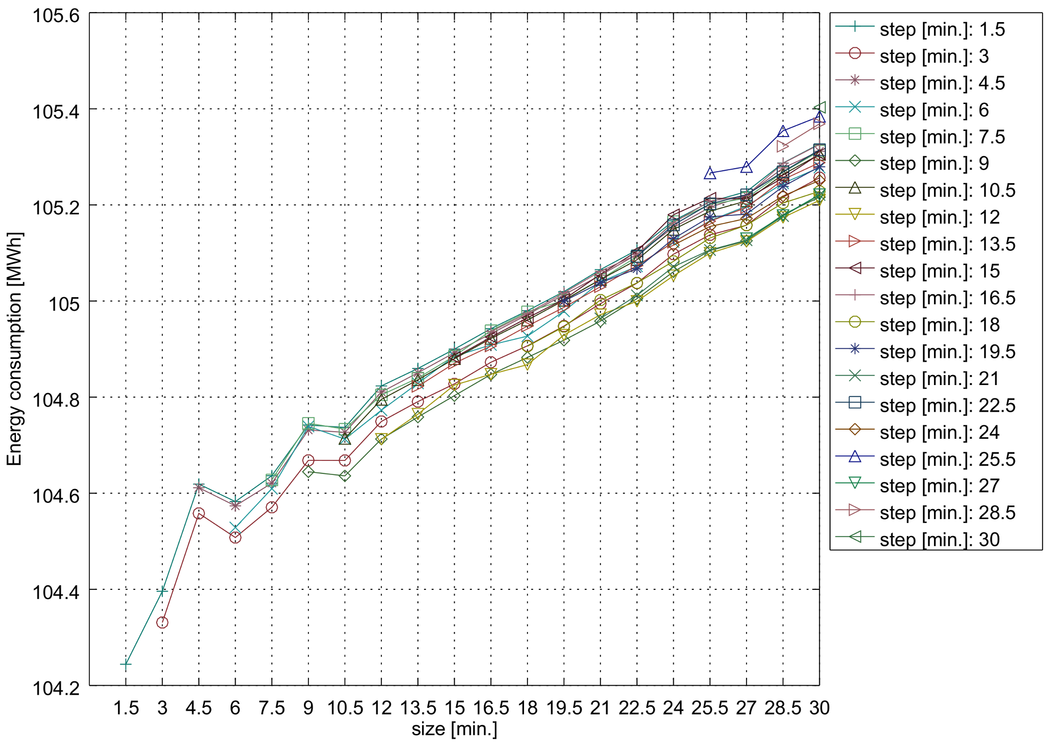More detailed results are presented in Figure 7, which enables easier identification of particular values. The worst result (the most energy consumed) was for the longest window size and step tested, which were equal to 30 min. The greatest energy savings were achieved for small sizes and steps, namely, 1.5 min. However, it needs to be pointed out that such small values are subject to aforementioned reliability issues caused by the traffic’s light cycle time and traffic jams. Additionally, using such a window would lead to an undesired effect of a visible and apparent fluctuation of lighting levels. It would impact safety, aesthetics and comfort.

Figure 7 gives a guideline to estimate the frequency of traffic intensity readings in terms of their economic viability. It has to be kept in mind that having high-frequency, accurate sensor data is desirable, but it comes with some cost. This is the cost of the devices, data transmission, communication hardware, storage and software licensing. Detailed window sizes and steps ordered by energy savings are given in

Table 3. Energy savings (%) and consumption (Wh) with different time window size (min) and step (min): ordered by the savings, the installation compliant with the CEN/TR 13201 2004 standard; typical and prospective sizes and steps are in bold.

Energy Saving	Energy Consumption	Size	Step	Energy Saving	Energy Consumption	Size	Step
27.19	104,244,133	1.50	1.50	26.79	104,825,094	15.00	12.00
27.13	104,331,020	3.00	3.00	26.79	104,827,602	15.00	3.00
27.09	104,396,012	3.00	1.50	26.79	104,828,757	13.50	6.00
27.01	104,507,834	6.00	3.00	26.78	104,836,034	13.50	10.50
27.00	104,528,675	6.00	6.00	26.78	104,839,572	13.50	7.50
26.98	104,558,063	4.50	3.00	26.77	104,847,208	16.50	9.00
26.97	104,570,737	7.50	3.00	26.77	104,847,529	16.50	12.00
26.96	104,573,755	6.00	4.50	26.77	104,850,669	13.50	4.50
26.96	104,582,646	6.00	1.50	26.76	104,859,612	13.50	1.50
26.94	104,609,467	7.50	6.00	26.76	104,867,556	18.00	12.00
26.94	104,611,447	4.50	4.50	26.76	104,870,538	15.00	13.50
26.93	104,618,977	4.50	1.50	26.76	104,872,598	16.50	3.00
26.93	104,621,037	7.50	4.50	26.75	104,879,850	15.00	10.50
26.93	104,627,737	7.50	7.50	26.75	104,882,218	15.00	15.00
26.92	104,636,128	10.50	9.00	26.75	104,882,584	18.00	9.00
26.92	104,636,548	7.50	1.50	26.75	104,884,969	15.00	6.00
26.91	104,644,680	9.00	9.00	26.75	104,885,496	15.00	7.50
26.90	104,668,194	10.50	3.00	26.74	104,892,451	15.00	4.50
26.90	104,668,380	9.00	3.00	26.74	104,899,905	15.00	1.50
26.87	104,712,165	12.00	12.00	26.73	104,905,835	18.00	18.00
26.87	104,712,592	10.50	6.00	26.73	104,906,494	16.50	13.50
26.87	104,712,810	12.00	9.00	26.73	104,906,764	18.00	3.00
26.87	104,714,042	10.50	10.50	26.73	104,908,685	16.50	6.00
26.86	104,726,766	10.50	4.50	26.72	104,918,446	19.50	9.00
26.85	104,731,530	9.00	4.50	26.72	104,922,062	16.50	10.50
26.85	104,733,236	10.50	7.50	26.72	104,924,829	16.50	15.00
26.85	104,736,888	10.50	1.50	26.72	104,926,889	18.00	6.00
26.85	104,739,167	9.00	6.00	26.72	104,929,168	19.50	12.00
26.85	104,741,898	9.00	1.50	26.71	104,931,966	16.50	4.50
26.84	104,745,543	9.00	7.50	26.71	104,936,360	16.50	16.50
26.84	104,749,379	12.00	3.00	26.71	104,938,219	16.50	7.50
26.84	104,758,577	13.50	9.00	26.71	104,942,449	16.50	1.50
26.83	104,764,605	13.50	12.00	26.70	104,946,673	19.50	18.00
26.83	104,772,861	12.00	6.00	26.70	104,947,946	18.00	13.50
26.81	104,790,691	13.50	3.00	26.70	104,947,962	19.50	3.00
26.81	104,795,278	12.00	10.50	26.70	104,958,104	21.00	9.00
26.80	104,803,041	15.00	9.00	26.69	104,960,188	18.00	10.50
26.80	104,804,634	12.00	7.50	26.69	104,963,740	21.00	21.00
26.80	104,810,617	12.00	4.50	26.69	104,964,876	18.00	15.00
26.79	104,822,414	13.50	13.50	…	…	…	…
26.79	104,823,331	12.00	1.50	26.38	105,403,071	30.00	30.00

. The savings are expressed as percentages of the reference energy usage with no dynamic control. The actual energy consumption is also given for reference. The maximum energy consumption is 105,403,071 Wh/year, with the window size and step at 30 min. The minimum energy consumption is 104,244,133 Wh/year, with the window size and step at 1.5 min. The maximum and minimum energy consumption differ only by 1.1% from each other. However, taking into consideration a city-wide deployment at 60,000 luminaires, this would yield over 214 MWh of energy savings each year. Thus, depending on the deployment scale, the benefits, in the form of energy saving, become apparent. They can overcome the cost related to more frequent readouts from the sensor systems.

We summarize the findings for the 2004 standard. A commonly used window size and step is 15 min. This yields 104,882,218 Wh, which is 26.75% of energy savings if compared with the reference with no dynamic control. Promising results can be obtained by having a window size of 6 min. with a step of 3 min., yielding energy usage at 104,507,834 Wh, which translates to 27.01%, or 6 and 6 min. with 104,528,675 Wh, being 27.00%. If this measurement frequency is too costly, a next measurement to consider is 10.5 min. with a step of 9 min., yielding 104,636,128 Wh, translating to 26.92%, or the marginally worse 9 and 9 min., with 104,644,680 Wh. These results are presented in Table 3 in bold.

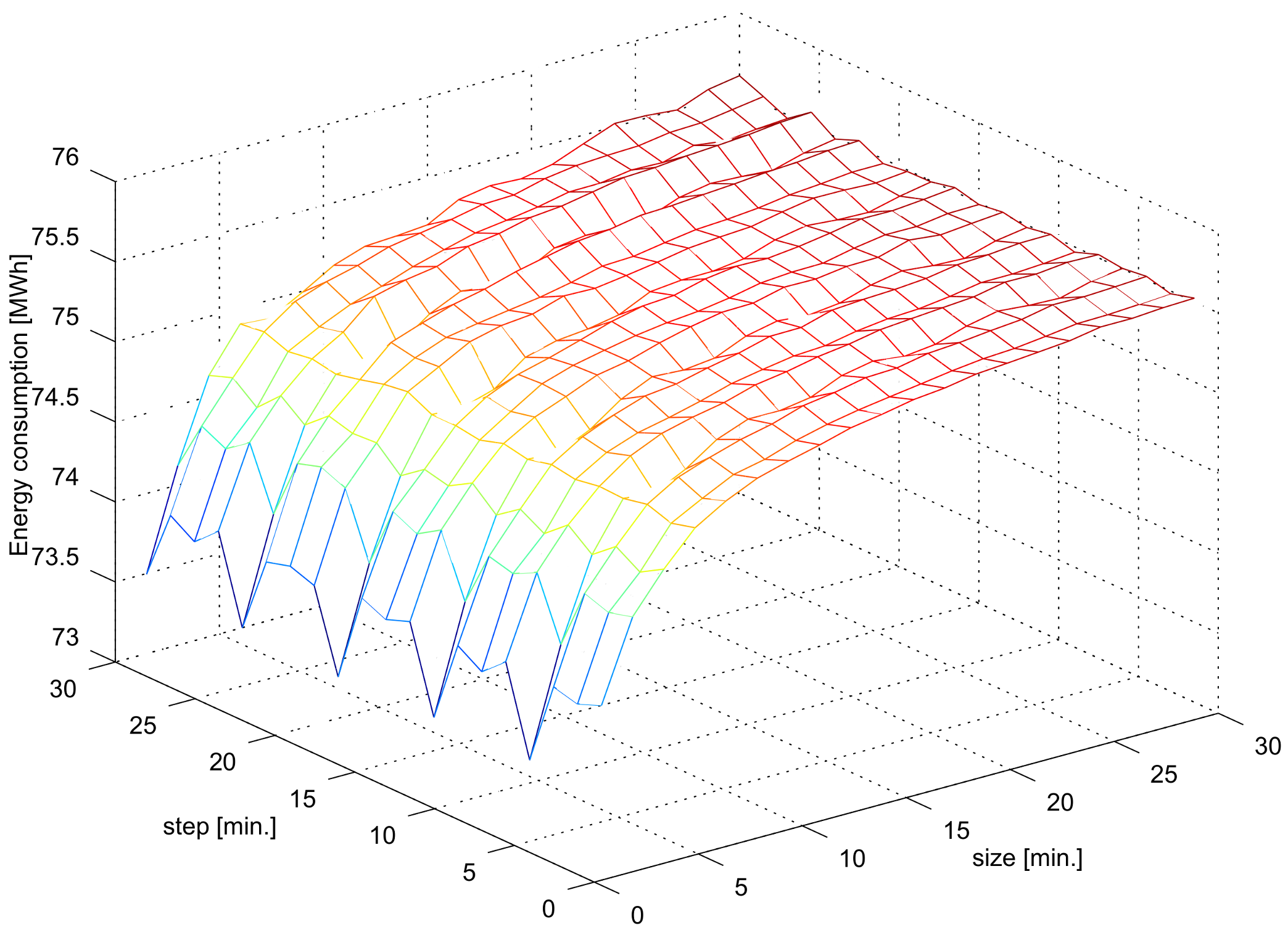
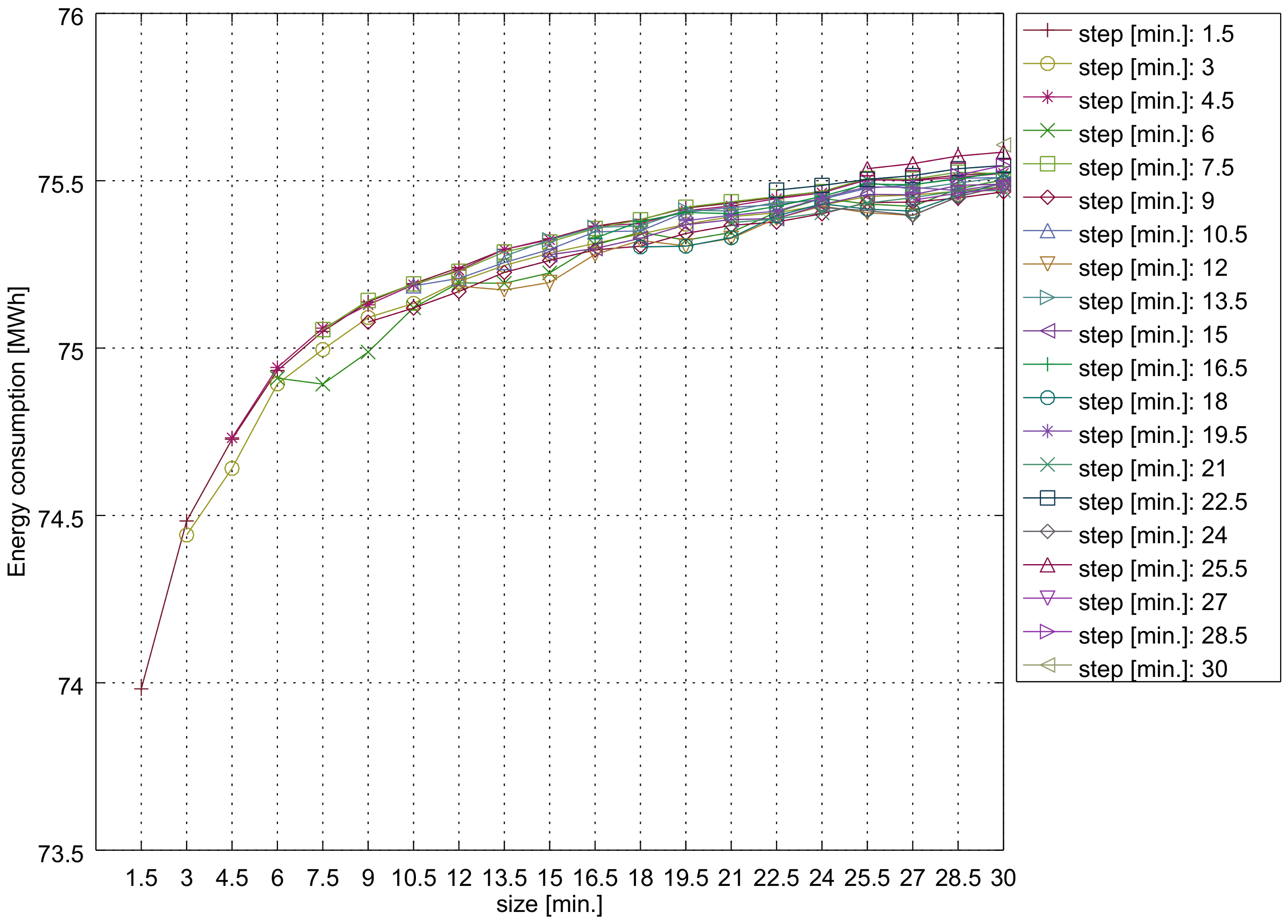
The reference energy usage for the CEN/TR 13201 2014 standard is the same as for the 2004 standard, which is 143,191,110 Wh. Applying a typical window size and step equal to 15 min indicates energy consumption at 75,278,974 Wh. It yields 47.43% of energy savings compared with the reference. A comparison of the different moving window sizes and steps’ overview is given in Figure 8, with a more detailed diagram in Figure 9 and particular values in

Table 4. Energy savings (%) and consumption (Wh) with different time window size (min) and step (min); ordered by the savings, the installation compliant with the CEN/TR 13201 2014 standard, typical and prospective sizes and steps are in bold.

Energy Saving	Energy Consumption	Size	Step	Energy Saving	Energy Consumption	Size	Step
48.33	73,981,862	1.50	1.50	47.45	75,246,738	13.50	3.00
48.01	74,441,605	3.00	3.00	47.44	75,255,460	13.50	10.50
47.98	74,483,398	3.00	1.50	47.44	75,261,756	15.00	9.00
47.87	74,640,570	4.50	3.00	47.43	75,274,712	13.50	13.50
47.81	74,727,749	4.50	1.50	47.43	75,278,974	15.00	15.00
47.81	74,731,862	4.50	4.50	47.43	75,279,940	16.50	12.00
47.70	74,892,350	7.50	6.00	47.42	75,283,685	15.00	3.00
47.70	74,893,002	6.00	3.00	47.42	75,287,177	13.50	7.50
47.69	74,910,090	6.00	6.00	47.42	75,293,378	16.50	9.00
47.67	74,933,113	6.00	1.50	47.42	75,294,654	13.50	1.50
47.66	74,942,074	6.00	4.50	47.42	75,294,820	13.50	4.50
47.63	74,988,222	9.00	6.00	47.42	75,294,977	15.00	10.50
47.63	74,995,698	7.50	3.00	47.41	75,297,583	16.50	15.00
47.59	75,049,758	7.50	1.50	47.41	75,302,259	18.00	18.00
47.58	75,055,338	7.50	7.50	47.41	75,304,565	18.00	9.00
47.58	75,059,594	7.50	4.50	47.41	75,304,592	19.50	18.00
47.57	75,077,612	9.00	9.00	47.41	75,305,269	19.50	12.00
47.56	75,091,435	9.00	3.00	47.41	75,308,192	16.50	6.00
47.54	75,119,812	10.50	9.00	47.40	75,312,939	16.50	3.00
47.54	75,120,543	10.50	6.00	47.40	75,317,053	15.00	7.50
47.53	75,129,439	9.00	4.50	47.40	75,321,712	18.00	12.00
47.53	75,133,466	10.50	3.00	47.40	75,322,502	19.50	6.00
47.53	75,137,940	9.00	1.50	47.40	75,323,295	15.00	13.50
47.52	75,142,345	9.00	7.50	47.40	75,323,961	15.00	4.50
47.50	75,169,011	12.00	9.00	47.39	75,326,361	15.00	1.50
47.50	75,173,506	13.50	12.00	47.39	75,327,645	21.00	12.00
47.49	75,185,042	12.00	12.00	47.39	75,328,034	18.00	15.00
47.49	75,186,072	10.50	10.50	47.39	75,328,681	16.50	16.50
47.49	75,189,252	10.50	4.50	47.39	75,329,974	21.00	18.00
47.49	75,191,803	10.50	7.50	47.38	75,340,764	18.00	3.00
47.49	75,192,687	10.50	1.50	47.38	75,342,424	19.50	9.00
47.49	75,193,637	13.50	6.00	47.38	75,345,467	21.00	6.00
47.49	75,194,868	12.00	6.00	47.38	75,346,169	18.00	6.00
47.49	75,195,989	15.00	12.00	47.38	75,347,345	16.50	10.50
47.48	75,198,830	12.00	3.00	47.38	75,349,926	18.00	10.50
47.48	75,208,382	12.00	10.50	47.37	75,357,425	16.50	7.50
47.47	75,224,605	15.00	6.00	47.37	75,360,567	16.50	13.50
47.46	75,226,080	13.50	9.00	47.37	75,364,173	16.50	4.50
47.46	75,229,516	12.00	7.50	47.37	75,364,354	16.50	1.50
47.46	75,232,910	12.00	4.50	…	…	…	…
47.45	75,240,380	12.00	1.50	47.20	75,607,209	30.00	30.00

—ordered according to the energy consumption. The maximum energy consumption is 75,607,209 Wh/year, with the window size and step at 30 min. The minimum energy consumption is 73,981,862 Wh/year, with the window size and step at 1.5 min. The maximum and minimum energy consumption differ by 2.1% from each other. However, taking into consideration a city-wide deployment at 60,000 luminaires, this would yield over 185 MWh of energy savings each year.

We summarize the findings for the 2014 standard. Promising results can be obtained having the window size of 7.5 min. with a step of 6 min., yielding energy usage at 74,892,350 Wh, which is 47.70%, or the slightly worse 6 and 6 min., with 74,910,090 Wh, being 47.69%. If this measurement frequency is too costly, a next measurement to consider is 9 and 9 min., yielding 75,077,612 Wh, translating to 47.57%. These results are presented in Table 4 in bold.

It needs to be noted that, besides the energy savings due to different window steps and sizes, applying the 2014 standard for a dynamic control leads to far greater savings than the 2004 standard for the same infrastructure. This is yet another economic argument for the deployment of lighting control systems. The increase in savings is due to two factors. First, the traffic volume at which lighting class switching can take place is in relation to the maximum capacity for the 2014 standard, as opposed to fixed values for the 2004 standard. Second, the lighting class can be lowered by two as a result of a traffic volume decrease, for any normal class, as can be seen in Table 2. Such lowering can take place only for some classes on the basis of lighting situation sets for the 2004 standard.

The actual costs of lighting control and sensor systems are not considered here. This is due to significant price differences even for the same luminaires or sensors for different deployments. Luminaire prices from a single vendor can differ by up to 50%. To equip a luminaire with a remote control increases its price by 0–142 EUR. Because of the above, any cost-based comparison would be subject to significant errors.

6. Conclusions

The economic feasibility of dynamic street lighting is based on a balance between energy savings and the cost of obtaining sensor data. The paper investigates, on a representative test case, how data source parameters influence these savings. It can serve as a guideline to select proper cost-wise parameters for how frequently traffic intensity information should be read. It offers a support to make economically viable decisions while designing intelligent outdoor lighting.

The research was carried out using 324 lighting fixtures and 107 induction loops, in Kraków, Poland. The energy consumption was calculated by using a simulation of the aforementioned infrastructure. It utilized a graph-based dynamic control system, which ensured compliance with the lighting standards. Thus, all safety requirements regarding lighting intensity were met at any time. Different data source parameters such as the averaging window sizes and steps were simulated. Their influence on the energy consumption reduction was verified.

The case was analyzed with the use of the 2004 and 2014 lighting standards. When the deployment was in accordance with the CEN/TR 13201 2004 standard and assuming a typical window step and size equal to 15 min [5,19], it resulted in energy savings of 26.75% . Decreasing these to 9 min returned 26.92%. Decreasing these further to 6 min resulted in 27.00%. These results are presented in Table 3 in bold. When the deployment was in accordance with the CEN/TR 13201 2014 standard, the 15 min step and size resulted in 47.43%. Decreasing these to 9 and 9 min. provided 47.57%, and decreasing these even further to 6 and 6 min. returned 47.69%. The above percentages can be further used as a guideline to verify if investment in more capable sensor infrastructure is viable.

An additional observation should be made that, for the dynamic control, the 2014 standard provided greater energy efficiency than the 2004 standard. This was due to an improved lighting class switching schema. This could serve as a convincing argument to redesign existing remotely controlled installations to make them compliant with the 2014 standard, particularly given that the cost of such a redesign would be a fraction of the actual savings due to decreased energy consumption.

The research was carried out using LED light sources. Thus, it was based on the assumptions that the dimming of a light source does not reduce its life span, and that there is a linear relationship between the light intensity and energy consumption over a wide range of power settings from 20% to 100%. Such characteristics are out of reach for older technologies such as HPS. Thus, the results confirm that choosing LEDs gives yet greater economic leverage for more energy efficient and sustainable living.

To summarize:

• the lighting standard compliant dynamic control of street lighting on the basis of traffic intensity detection results in substantial energy saving;
• the savings depend on traffic intensity measurement parameters: the moving window size and step;
• the cost of traffic intensity detection is also based on the moving window size and step;
• the proposed guidelines (see Table 3 and Table 4) indicate that the shorter the window size and step, the greater the savings achievable;
• there are two sets of the guidelines for both the previous (2004) and current (2014) CEN/TR 13201 standards to make them applicable to existing and future deployments;
• there are substantially greater savings if the installation is compliant with the CEN/TR 13201 2014 compared to the CEN/TR 13201 2004 standard.

Further research focuses on the analysis of extending environmental parameters, and finding economically viable conditions for applying the dynamic street lighting control. These parameters include ambient or vehicle lights [23,24], as well as weather conditions. It needs to be pointed out that there is a feedback between vehicle lights and street or road lighting, which results in complex interactions between them [25,26,27]. The main challenge is to obtain reliable data. Incorporating this into the existing model does not pose any difficulty, as the model is capable of accepting diverse sensor data sources by design, as was mentioned before.