Geographically Weighted Regression Models in Estimating Median Home Prices in Towns of Massachusetts Based on an Urban Sustainability Framework


Abstract
1. Introduction
1.1. Background
1.2. Modeling Framework
2. Materials and Methods
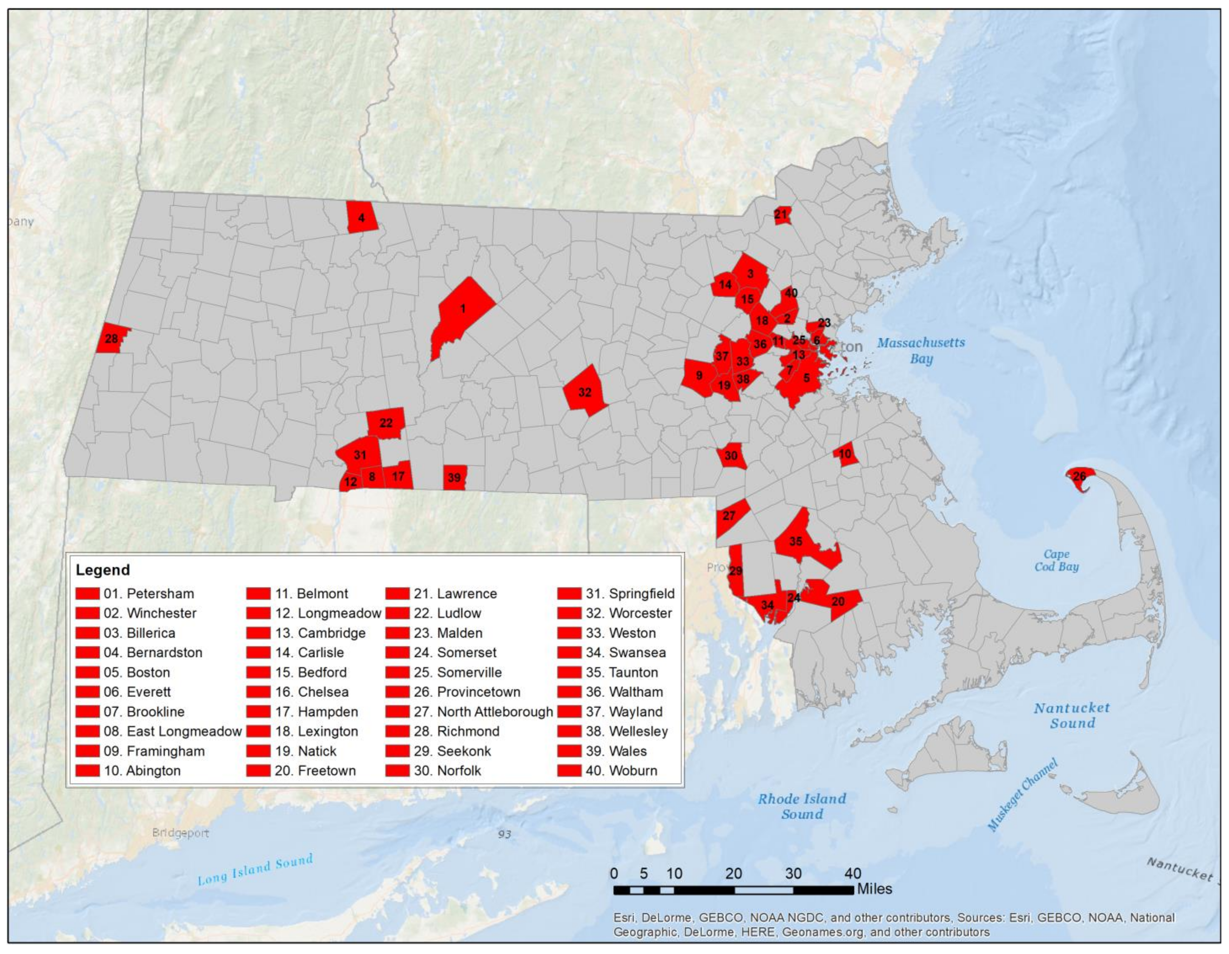
2.1. Study Area
2.2. Data Sources—Socio-Economic and Environmental Variables
2.3. Spatial Model Considerations
- is the dependent variable at location
- is the th independent variable at location
- is the number of independent variables
3. Results
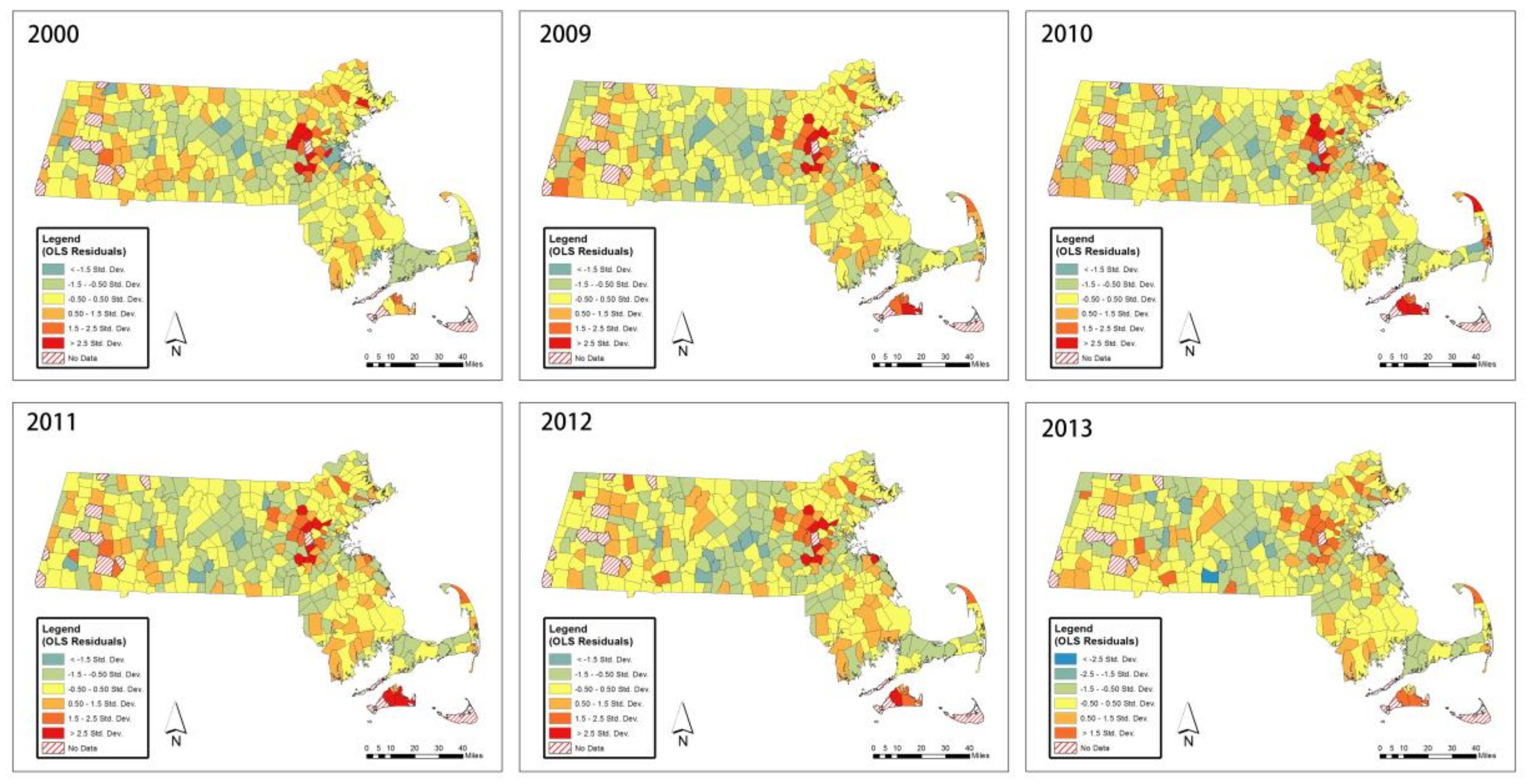
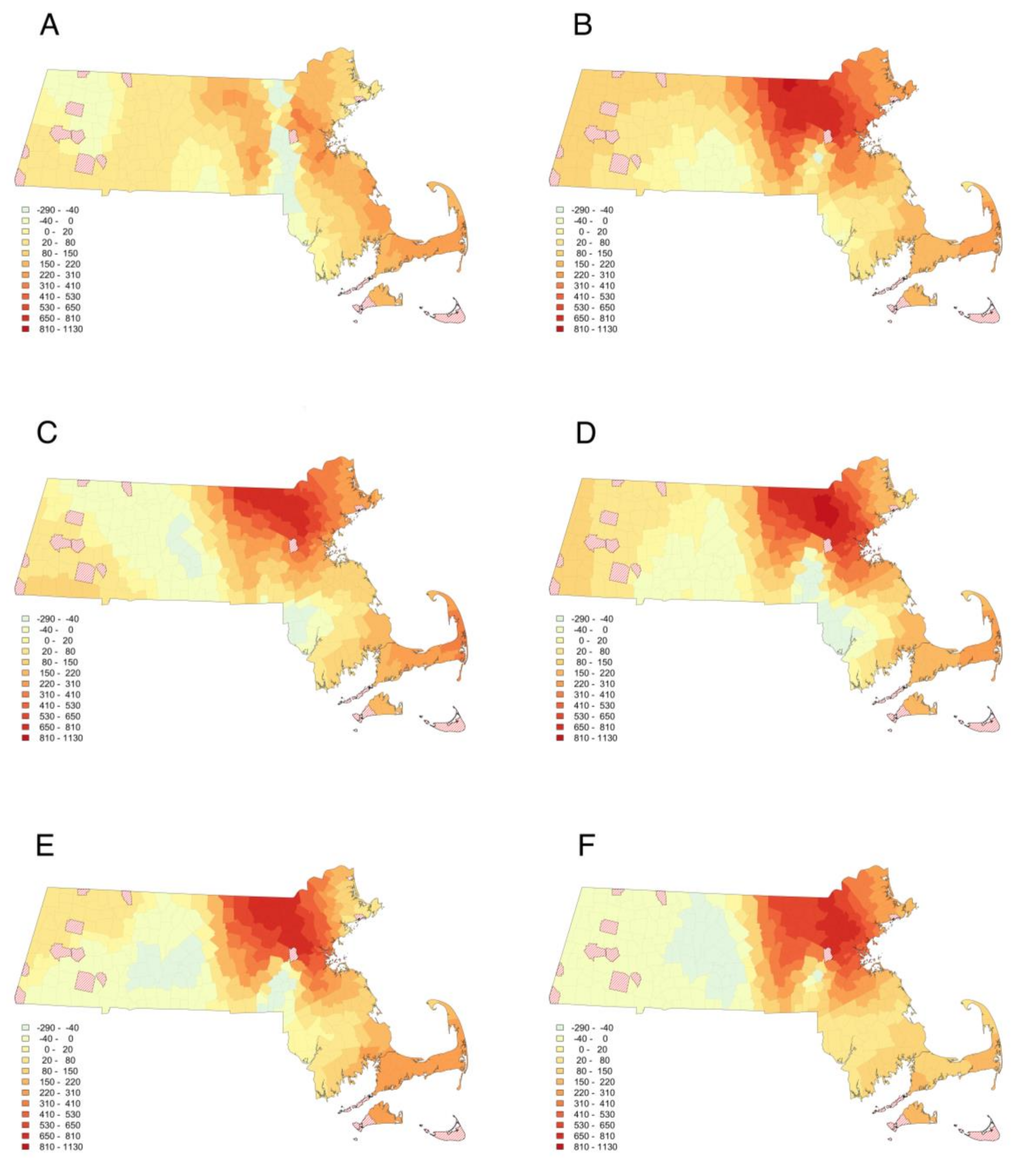
3.1. Spatial-Temporal Patterns of Home Prices
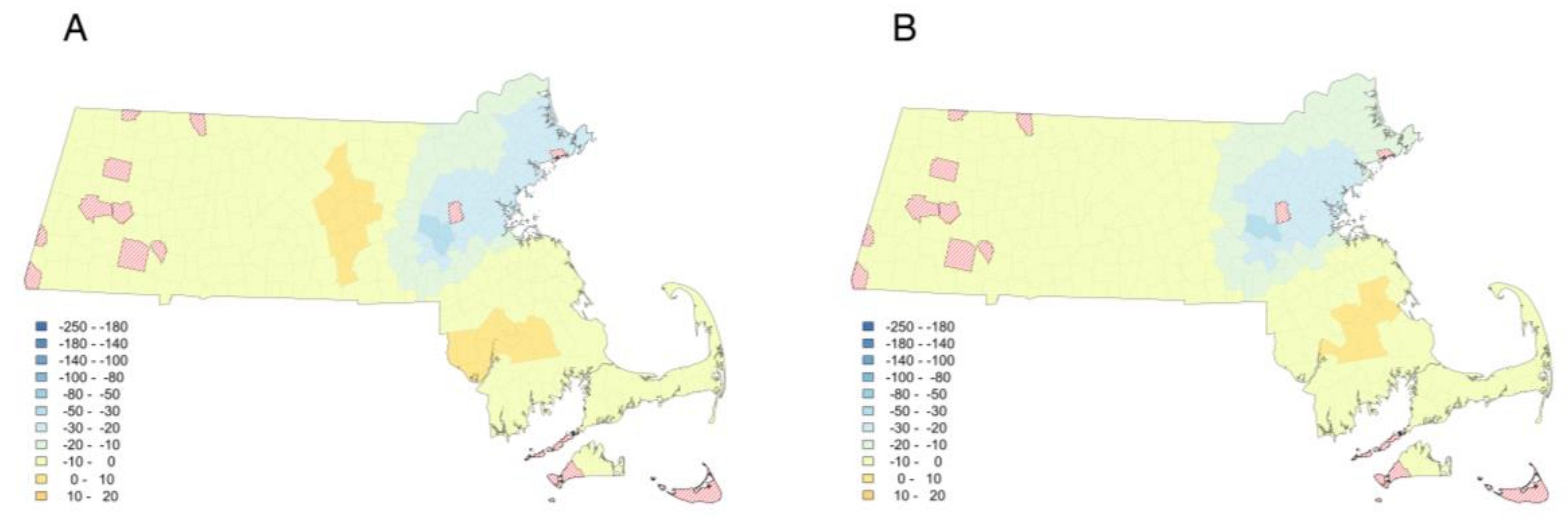
3.2. Are All Determinants of Median Home Price Non-Stationary?
3.3. Impact of Housing on Urban Sustainability
4. Discussion
5. Conclusions
Supplementary Materials
Acknowledgments
Author Contributions
Conflicts of Interest
Appendix A

| Median Home Price | |||||||
|---|---|---|---|---|---|---|---|
| Basic GWR Model (2000) | |||||||
| Variables | Minimum | Median | Max | % of Positive | % of Negative | p-Value (F3) | Sig. |
| Intercept | −212.70 | 243.24 | 1190.76 | 90.77 | 9.23 | 1.47 × 10⁻¹¹ | *** |
| Population Density | −11.92 | 0.68 | 28.78 | 60.71 | 39.29 | 0.5142965 | - |
| Unprotected Forest | −217.68 | 68.88 | 388.90 | 84.52 | 15.48 | 0.3060173 | - |
| Unemployment Rate | −189.08 | −17.66 | 16.92 | 11.31 | 88.69 | <2.2 × 10⁻¹⁶ | *** |
| Residential Area | −756.43 | −73.39 | 300.69 | 35.71 | 64.29 | 0.0004993 | *** |
| Vehicle ownership | −1323.53 | −162.52 | 229.86 | 9.82 | 90.18 | <2.2 × 10⁻¹⁶ | *** |
| Higher Education | 297.39 | 1110.62 | 1985.25 | 100 | 0 | 6.85 × 10⁻¹³ | *** |
| Senior Population | −522.05 | 226.41 | 1470.80 | 84.82 | 15.18 | 1.04 × 10⁻¹¹ | *** |
| Dist. to Stations | −8.48 | −0.18 | 16.72 | 39.88 | 60.12 | 3.59 × 10⁻⁶ | *** |
| Property Tax | −20.63 | −3.48 | 1.38 | 10.12 | 89.88 | 6.51 × 10⁻¹² | *** |
| CPI | −1.37 | 1.38 | 6.78 | 80.65 | 19.35 | 0.040276 | * |
| Median Home Price | |||||||
|---|---|---|---|---|---|---|---|
| Basic GWR Model (2010) | |||||||
| Variables | Minimum | Median | Max | % of Positive | % of Negative | p-Value (F3) | Sig. |
| Intercept | −130.54 | 347.02 | 1501.33 | 97.92 | 2.08 | 3.07 × 10⁻² | * |
| Population Density | −11.22 | 2.30 | 25.15 | 78.27 | 21.73 | 0.531882 | - |
| Unprotected Forest | −61.80 | 100.84 | 745.17 | 77.08 | 22.92 | 1.90 × 10⁻¹³ | *** |
| Unemployment Rate | −114.97 | −15.33 | 3.10 | 2.68 | 97.32 | <2.2 × 10⁻¹⁶ | *** |
| Residential Area | −781.96 | −107.39 | 246.64 | 33.63 | 66.37 | 4.49 × 10⁻⁹ | *** |
| Vehicle ownership | −872.92 | −274.53 | 64.77 | 2.08 | 97.92 | 1.57 × 10⁻⁷ | *** |
| Higher Education | −2067.55 | 626.96 | 2327.99 | 88.99 | 11.01 | <2.2 × 10⁻¹⁶ | *** |
| Senior Population | −409.73 | 660.41 | 2574.71 | 83.63 | 16.37 | <2.2 × 10⁻¹⁶ | *** |
| Dist. to Stations | −18.26 | −2.00 | 3.39 | 25 | 75 | <2.2 × 10⁻¹⁶ | *** |
| Property Tax | −29.32 | −7.03 | 2.51 | 4.17 | 95.83 | 3.94 × 10⁻³ | ** |
| CPI | −3.72 | 3.59 | 17.98 | 87.5 | 12.5 | 0.043231 | * |
| Median Home Price | |||||||
|---|---|---|---|---|---|---|---|
| Basic GWR Model (2009) | |||||||
| Variables | Minimum | Median | Max | % of Positive | % of Negative | p-Value (F3) | Sig. |
| Intercept | −1507.61 | −34.44 | 433.69 | 44.94 | 55.06 | 3.91 × 10⁻⁵ | *** |
| Population Density | −10.47 | 5.07 | 30.88 | 89.88 | 10.12 | 0.2161 | - |
| Unprotected Forest | −59.97 | 141.74 | 812.44 | 93.45 | 6.55 | <2.2 × 10⁻¹⁶ | *** |
| Unemployment Rate | −29.38 | −3.14 | 17.12 | 21.43 | 78.57 | 7.21 × 10⁻⁸ | *** |
| Residential Area | −842.60 | −139.32 | 242.05 | 15.18 | 84.82 | 4.40 × 10⁻⁵ | *** |
| Vehicle ownership | −1018.52 | −300.08 | 126.04 | 2.98 | 97.02 | 5.52 × 10⁻⁷ | *** |
| Higher Education | −545.12 | 1083.32 | 2578.53 | 97.92 | 2.08 | <2.2 × 10⁻¹⁶ | *** |
| Senior Population | −625.56 | 537.45 | 2741.07 | 82.14 | 17.86 | <2.2 × 10⁻¹⁶ | *** |
| Dist. to Stations | −12.16 | −2.29 | 3.16 | 26.19 | 73.81 | 1.90 × 10⁻⁵ | *** |
| Property Tax | −37.52 | −7.63 | 8.01 | 7.44 | 92.56 | 7.09 × 10⁻⁸ | *** |
| CPI | 0.09 | 5.47 | 28.54 | 100 | 0 | <2.2 × 10⁻¹⁶ | *** |
| Median Home Price | |||||||
|---|---|---|---|---|---|---|---|
| Basic GWR Model (2011) | |||||||
| Variables | Minimum | Median | Max | % of Positive | % of Negative | p-Value (F3) | Sig. |
| Intercept | −1213.56 | 1.45 | 339.49 | 50.6 | 49.4 | 5.81 × 10⁻¹ | - |
| Population Density | −7.34 | 6.93 | 31.59 | 92.86 | 7.14 | 0.2586052 | - |
| Unprotected Forest | −154.56 | 97.60 | 857.46 | 79.76 | 20.24 | <2.2 × 10⁻¹⁶ | *** |
| Unemployment Rate | −35.99 | −7.29 | 2.88 | 1.79 | 98.21 | 1.72 × 10⁻⁸ | *** |
| Residential Area | −950.93 | −169.73 | 147.89 | 9.23 | 90.77 | 1.03 × 10⁻³ | ** |
| Vehicle ownership | −860.20 | −253.15 | 99.18 | 2.38 | 97.62 | 1.93 × 10⁻³ | ** |
| Higher Education | −1494.37 | 800.34 | 2474.53 | 94.94 | 5.06 | <2.2 × 10⁻¹⁶ | *** |
| Senior Population | −567.12 | 539.88 | 2330.52 | 87.5 | 12.5 | <2.2 × 10⁻¹⁶ | *** |
| Dist. to Stations | −9.94 | −1.14 | 3.57 | 24.4 | 75.6 | 1.58 × 10⁻¹ | - |
| Property Tax | −25.86 | −5.60 | 3.56 | 3.87 | 96.13 | 9.45 × 10⁻⁴ | *** |
| CPI | −0.22 | 4.12 | 25.70 | 99.4 | 0.6 | 1.20 × 10⁻¹³ | *** |
| Median Home Price | |||||||
|---|---|---|---|---|---|---|---|
| Basic GWR Model (2012) | |||||||
| Variables | Minimum | Median | Max | % of Positive | % of Negative | p-Value (F3) | Sig. |
| Intercept | −918.93 | −27.37 | 341.96 | 46.13 | 53.87 | 4.86 × 10⁻¹ | - |
| Population Density | −8.03 | 7.73 | 40.81 | 92.56 | 7.44 | 0.005703 | ** |
| Unprotected Forest | −191.22 | 94.72 | 770.02 | 75 | 25 | < 2.2 × 10⁻¹⁶ | *** |
| Unemployment Rate | −40.78 | −7.78 | 4.25 | 4.46 | 95.54 | 2.99 × 10⁻¹⁶ | *** |
| Residential Area | −1178.58 | −203.18 | 144.67 | 9.23 | 90.77 | 3.64 × 10⁻⁶ | *** |
| Vehicle ownership | −742.86 | −222.69 | 93.19 | 13.39 | 86.61 | 6.33 × 10⁻⁵ | *** |
| Higher Education | −1489.48 | 837.34 | 2527.95 | 94.35 | 5.65 | < 2.2 × 10⁻¹⁶ | *** |
| Senior Population | −477.13 | 481.55 | 2309.47 | 87.5 | 12.5 | 5.66 × 10⁻¹⁵ | *** |
| Dist. to Stations | −11.23 | −0.94 | 10.82 | 29.17 | 70.83 | 9.25 × 10⁻⁵ | *** |
| Property Tax | −26.11 | −5.16 | 5.01 | 3.57 | 96.43 | 8.22 × 10⁻⁹ | *** |
| CPI | 0.76 | 4.62 | 23.77 | 100 | 0 | < 2.2 × 10⁻¹⁶ | *** |
| Median Home Price | |||||||
|---|---|---|---|---|---|---|---|
| Basic GWR Model (2013) | |||||||
| Variables | Minimum | Median | Max | % of Positive | % of Negative | p-Value (F3) | Sig. |
| Intercept | −748.02 | −159.96 | 279.56 | 30.95 | 69.05 | 9.71 × 10⁻¹ | - |
| Population Density | −7.81 | 7.60 | 41.48 | 93.15 | 6.85 | 1.43 × 10⁻⁶ | *** |
| Unprotected Forest | −63.64 | 120.01 | 768.53 | 65.77 | 34.23 | <2.2 × 10⁻¹⁶ | *** |
| Unemployment Rate | −32.81 | −6.94 | 2.92 | 6.55 | 93.45 | 3.50 × 10⁻¹² | *** |
| Residential Area | −937.70 | −202.99 | 148.44 | 13.1 | 86.9 | 9.43 × 10⁻⁶ | *** |
| Vehicle ownership | −796.82 | −259.97 | 519.41 | 5.65 | 94.35 | 1.62 × 10⁻⁸ | *** |
| Higher Education | −537.89 | 843.47 | 1975.59 | 97.62 | 2.38 | <2.2 × 10⁻¹⁶ | *** |
| Senior Population | −408.29 | 656.82 | 2340.80 | 91.96 | 8.04 | <2.2 × 10⁻¹⁶ | *** |
| Dist. to Stations | −10.98 | −0.95 | 10.05 | 25 | 75 | 8.52 × 10⁻⁶ | *** |
| Property Tax | −21.75 | −5.72 | 1.91 | 8.33 | 91.67 | 7.10 × 10⁻⁹ | *** |
| CPI | 1.05 | 6.42 | 20.66 | 100 | 0 | 2.01 × 10⁻⁵ | *** |
| Median Home Price | |||||||
|---|---|---|---|---|---|---|---|
| Mixed GWR Model (2000) | |||||||
| Local Variables | |||||||
| Variables | Minimum | Median | Max | % of Positive | % of Negative | p-Value (MC) | Sig. |
| Intercept | −47.18 | 212.41 | 1440.56 | 94.64 | 5.36 | 0.04 | . |
| Population Density | −8.63 | 1.26 | 25.85 | 63.39 | 36.61 | 0.00 | *** |
| Unemployment Rate | −244.13 | −24.55 | 13.49 | 23.21 | 76.79 | 0.00 | *** |
| Residential Area | −730.09 | −98.82 | 279.04 | 34.23 | 65.77 | 0.00 | *** |
| Vehicle ownership | −1352.88 | −208.48 | 304.02 | 11.61 | 88.39 | 0.00 | *** |
| Senior Population | −528.56 | 179.11 | 1395.85 | 77.38 | 22.62 | 0.00 | *** |
| Dist. to Stations | −8.04 | −0.27 | 14.43 | 34.23 | 65.77 | 0.00 | *** |
| Property Tax | −17.89 | −3.25 | 0.84 | 10.42 | 89.58 | 0.04 | . |
| Global Variables | - | - | - | - | - | - | - |
| Unprotected Forest | - | - | - | 72.49 | - | 0.48 | - |
| Higher Education | - | - | - | 1063.50 | - | 0.11 | - |
| CPI | - | - | - | 1.08 | - | 0.32 | - |
| Median Home Price | |||||||
|---|---|---|---|---|---|---|---|
| Mixed GWR Model (2009) | |||||||
| Local Variables | |||||||
| Variables | Minimum | Median | Max | % of Positive | % of Negative | p-Value (MC) | Sig. |
| Population Density | 1.68 | 6.92 | 14.98 | 100 | 0 | 0.01 | . |
| Unprotected Forest | −18.47 | 136.56 | 877.81 | 97.02 | 2.98 | 0.01 | . |
| Unemployment Rate | −32.56 | −4.52 | 5.24 | 9.52 | 90.48 | 0.04 | . |
| Higher Education | −46.09 | 1027.44 | 2162.85 | 99.7 | 0.3 | 0.01 | . |
| Senior Population | −717.27 | 543.89 | 2525.48 | 84.82 | 15.18 | 0.00 | *** |
| Dist. to Stations | −17.40 | −2.75 | 4.61 | 26.79 | 73.21 | 0.00 | *** |
| Property Tax | 1.29 | 5.19 | 9.59 | 100 | 0 | 0.01 | . |
| Global Variables | - | - | - | - | - | - | - |
| Intercept | - | - | - | −22.98 | - | 0.23 | - |
| Residential Area | - | - | - | −192.74 | - | 0.08 | - |
| Vehicle ownership | - | - | - | −263.5063 | - | 0.21 | - |
| Property Tax | - | - | - | −6.2983 | - | 0.19 | - |
| Median Home Price | |||||||
|---|---|---|---|---|---|---|---|
| Mixed GWR Model (2010) | |||||||
| Local Variables | |||||||
| Variables | Minimum | Median | Max | % of Positive | % of Negative | p-Value (MC) | Sig. |
| Population Density | −10.61 | 3.01 | 23.37 | 75.6 | 24.4 | 0.00 | *** |
| Unprotected Forest | −117.24 | 81.15 | 1128.29 | 82.14 | 17.86 | 0.02 | . |
| Unemployment Rate | −78.05 | −17.19 | −3.43 | 0 | 100 | 0.00 | *** |
| Residential Area | −693.29 | −89.47 | 238.38 | 27.38 | 72.62 | 0.01 | . |
| Higher Education | −50.24 | 901.48 | 1603.10 | 99.7 | 0.3 | 0.00 | *** |
| Senior Population | −676.64 | 641.03 | 3500.10 | 77.68 | 22.32 | 0.00 | *** |
| Dist. to Stations | −20.46 | −1.46 | 4.61 | 20.54 | 79.46 | 0.00 | *** |
| Global Variables | - | - | - | - | - | - | - |
| Intercept | - | - | - | 273.3707 | - | 0.45 | - |
| Vehicle ownership | - | - | - | −243.0027 | - | 0.13 | - |
| Property Tax | - | - | - | −4.75 | - | 0.51 | - |
| CPI | - | - | - | 273.37 | - | 0.53 | - |
| Median Home Price | |||||||
|---|---|---|---|---|---|---|---|
| Mixed GWR Model (2011) | |||||||
| Local Variables | |||||||
| Variables | Minimum | Median | Max | % of Positive | % of Negative | p-Value (MC) | Sig. |
| Population Density | −3.65 | 7.91 | 31.49 | 95.54 | 4.46 | 0.01 | . |
| Unprotected Forest | −283.68 | 121.03 | 783.88 | 91.37 | 8.63 | 0.00 | *** |
| Residential Area | −970.74 | −192.49 | 132.06 | 6.55 | 93.45 | 0.00 | *** |
| Higher Education | −150.67 | 936.71 | 2298.48 | 99.11 | 0.89 | 0.00 | *** |
| Senior Population | −456.07 | 496.82 | 2273.67 | 88.1 | 11.9 | 0.00 | *** |
| Dist. to Stations | −13.77 | −1.91 | 3.66 | 18.15 | 81.85 | 0.00 | *** |
| CPI | −1.25 | 4.93 | 9.95 | 97.62 | 2.38 | 0.00 | *** |
| Global Variables | - | - | - | - | - | - | - |
| Intercept | - | - | - | −18.07 | - | - | - |
| Unemployment Rate | - | - | - | −7.38 | - | - | - |
| Vehicle ownership | - | - | - | −183.00 | - | - | - |
| Property Tax | - | - | - | −6.56 | - | - | - |
| Median Home Price | |||||||
|---|---|---|---|---|---|---|---|
| Mixed GWR Model (2012) | |||||||
| Local Variables | |||||||
| Variables | Minimum | Median | Max | % of Positive | % of Negative | p-Value (MC) | Sig. |
| Population Density | −7.00 | 9.36 | 42.00 | 97.62 | 2.38 | 0.00 | *** |
| Unprotected Forest | 0.77 | 85.71 | 712.42 | 100 | 100 | 0.00 | *** |
| Residential Area | −1101.51 | −262.61 | 198.37 | 5.65 | 94.35 | 0.00 | *** |
| Higher Education | −183.99 | 927.83 | 1689.29 | 99.7 | 0.3 | 0.00 | *** |
| Senior Population | −474.79 | 444.50 | 2876.72 | 84.23 | 15.77 | 0.00 | *** |
| Dist. to Stations | −17.50 | −1.10 | 4.17 | 20.83 | 79.17 | 0.00 | *** |
| Global Variables | - | - | - | - | - | - | - |
| Intercept | - | - | - | 7.78 | - | 0.77 | - |
| Unemployment Rate | - | - | - | −7.8404 | - | 0.06 | - |
| Vehicle ownership | - | - | - | −196.24 | - | 0.64 | - |
| Property Tax | - | - | - | −6.95 | - | 0.06 | - |
| CPI | - | - | - | 4.7264 | - | 0.05 | - |
| Median Home Price | |||||||
|---|---|---|---|---|---|---|---|
| Mixed GWR Model (2013) | |||||||
| Local Variables | |||||||
| Variables | Minimum | Median | Max | % of Positive | % of Negative | p-Value (MC) | Sig. |
| Population Density | −5.25 | 8.75 | 32.65 | 94.94 | 5.06 | 0.00 | *** |
| Unprotected Forest | −71.06 | 100.28 | 960.42 | 64.58 | 35.42 | 0.00 | *** |
| Unemployment Rate | −32.11 | −7.66 | 0.85 | 2.68 | 97.32 | 0.02 | . |
| Residential Area | −867.56 | −232.16 | 119.82 | 6.25 | 93.75 | 0.02 | . |
| Higher Education | 73.76 | 800.33 | 1532.83 | 100 | 0 | 0.01 | . |
| Senior Population | −606.89 | 584.40 | 2809.65 | 86.9 | 13.1 | 0.00 | *** |
| Dist. to Stations | −11.99 | −1.68 | 8.03 | 17.26 | 82.74 | 0.00 | *** |
| Property Tax | −19.62 | −7.01 | 1.37 | 5.06 | 94.94 | 0.03 | . |
| Global Variables | - | - | - | - | - | - | - |
| Intercept | - | - | - | −105.84 | - | 0.90 | - |
| Vehicle ownership | - | - | - | −206.13 | - | 0.24 | - |
| CPI | - | - | - | 6.03 | - | 0.37 | - |


References
- Pickett, S.; Burch, W., Jr.; Dalton, S.; Foresman, T.; Grove, J.; Rowntree, R. A conceptual framework for the study of human ecosystems in urban areas. Urban Ecosyst. 1997, 1, 185–199. [Google Scholar] [CrossRef]
- Grimm, N.; Grove, J.M.; Pickett, S.; Redman, C. Integrated Approaches to Long-Term Studies of Urban Ecological Systems. BioScience 2000, 50, 571–584. [Google Scholar] [CrossRef]
- Alberti, M. Modeling the urban ecosystem: A conceptual framework. Environ. Plan. B 1999, 26, 605–630. [Google Scholar] [CrossRef]
- Ostrom, E. A General Framework for Analyzing Sustainability of Social-Ecological Systems. Science 2009, 325, 419–422. [Google Scholar] [CrossRef] [PubMed]
- Newman, P.; Kenworthy, J. Sustainability and Cities; Island Press: Washington, DC, USA, 1999. [Google Scholar]
- Shiller, R. Understanding Recent Trends in House Prices and Home Ownership; Cowles Foundation for Research in Economics; Yale University: New Haven, CT, USA, 2007. [Google Scholar]
- Harris, D. “Property Values Drop When Blacks Move in, Because...”: Racial and Socioeconomic Determinants of Neighborhood Desirability. Am. Sociol. Rev. 1999, 64, 461–479. [Google Scholar] [CrossRef]
- Case, K.; Mayer, C. Housing price dynamics within a metropolitan area. Reg. Sci. Urban Econ. 1996, 26, 387–407. [Google Scholar] [CrossRef]
- Wolch, J.; Byrne, J.; Newell, J. Urban green space, public health, and environmental justice: The challenge of making cities ‘just green enough’. Landsc. Urban Plan. 2014, 125, 234–244. [Google Scholar] [CrossRef]
- Alkon, A.; Agyeman, J. Cultivating Food Justice; MIT Press: Cambridge, MA, USA, 2014. [Google Scholar]
- Cutts, B.; Darby, K.; Boone, C.; Brewis, A. City structure, obesity, and environmental justice: An integrated analysis of physical and social barriers to walkable streets and park access. Soc. Sci. Med. 2009, 69, 1314–1322. [Google Scholar] [CrossRef] [PubMed]
- Wu, B.; Li, R.; Huang, B. A geographically and temporally weighted autoregressive model with application to housing prices. Int. J. Geogr. Inf. Sci. 2014, 28, 1186–1204. [Google Scholar] [CrossRef]
- Wang, S.; Fang, C.; Wang, Y.; Huang, Y.; Ma, H. Quantifying the relationship between urban development intensity and carbon dioxide emissions using a panel data analysis. Ecol. Indic. 2015, 49, 121–131. [Google Scholar] [CrossRef]
- Wachsmuth, D.; Cohen, D.; Angelo, H. Expand the frontiers of urban sustainability. Nature 2016, 536, 391–393. [Google Scholar] [CrossRef] [PubMed]
- Goodman, A.; Thibodeau, T. Housing market segmentation and hedonic prediction accuracy. J. Hous. Econ. 2003, 12, 181–201. [Google Scholar] [CrossRef]
- LeSage, J. An Introduction to Spatial Econometrics. Revue D’économie Industrielle 2008, 123, 19–44. [Google Scholar] [CrossRef]
- Anselin, L. Spatial Econometrics; Springer: Dordrecht, The Netherlands, 2010. [Google Scholar]
- Huang, B.; Wu, B.; Barry, M. Geographically and temporally weighted regression for modeling spatio-temporal variation in house prices. Int. J. Geogr. Inf. Sci. 2010, 24, 383–401. [Google Scholar] [CrossRef]
- Bitter, C.; Mulligan, G.; Dall’erba, S. Incorporating spatial variation in housing attribute prices: A comparison of geographically weighted regression and the spatial expansion method. J. Geogr. Syst. 2006, 9, 7–27. [Google Scholar] [CrossRef]
- Helbich, M.; Brunauer, W.; Vaz, E.; Nijkamp, P. Spatial Heterogeneity in Hedonic House Price Models: The Case of Austria. Urban Stud. 2013, 51, 390–411. [Google Scholar] [CrossRef]
- Paulsen, K. The Effects of Growth Management on the Spatial Extent of Urban Development, Revisited. Land Econ. 2013, 89, 193–210. [Google Scholar] [CrossRef]
- Hasse, J.; Lathrop, R. A Housing-Unit-Level Approach to Characterizing Residential Sprawl. Photogramm. Eng. Remote Sens. 2003, 69, 1021–1030. [Google Scholar] [CrossRef]
- Collins, J.; Woodcock, C. An assessment of several linear change detection techniques for mapping forest mortality using multitemporal landsat TM data. Remote Sens. Environ. 1996, 56, 66–77. [Google Scholar] [CrossRef]
- Jeon, S.; Olofsson, P.; Woodcock, C. Land use change in New England: A reversal of the forest transition. J. Land Use Sci. 2013, 9, 105–130. [Google Scholar] [CrossRef]
- Kennedy, R.; Yang, Z.; Cohen, W. Detecting trends in forest disturbance and recovery using yearly Landsat time series: 1. LandTrendr—Temporal segmentation algorithms. Remote Sens. Environ. 2010, 114, 2897–2910. [Google Scholar] [CrossRef]
- Maliene, V.; Malys, N. High-quality housing—A key issue in delivering sustainable communities. Build. Environ. 2009, 44, 426–430. [Google Scholar] [CrossRef]
- Case, K.; Shiller, R. Is There a Bubble in the Housing Market? Brook. Pap. Econ. Act. 2003, 2003, 299–362. [Google Scholar] [CrossRef]
- Higgins, C.; Kanaroglou, P. Forty years of modelling rapid transit’s land value uplift in North America: Moving beyond the tip of the iceberg. Transp. Rev. 2016, 36, 610–634. [Google Scholar] [CrossRef]
- Goodman, C.; Mance, S. Employment loss and the 2007–09 recession: An overview. Mon. Labor Rev. 2011, 134, 3–12. [Google Scholar]
- Myers, D.; Ryu, S. Aging Baby Boomers and the Generational Housing Bubble: Foresight and Mitigation of an Epic Transition. J. Am. Plan. Assoc. 2008, 74, 17–33. [Google Scholar] [CrossRef]
- Gibbons, S.; Machin, S. Valuing school quality, better transport, and lower crime: Evidence from house prices. Oxf. Rev. Econ. Policy 2008, 24, 99–119. [Google Scholar] [CrossRef]
- Aughinbaugh, A. Patterns of Homeownership, Delinquency, and Foreclosure among Youngest Baby Boomers; Bureau of Labor Statistics: Washington, DC, USA, 2013.
- Fotheringham, A.; Crespo, R.; Yao, J. Geographical and Temporal Weighted Regression (GTWR). Geogr. Anal. 2015, 47, 431–452. [Google Scholar] [CrossRef]
- Anselin, L. GIS Research Infrastructure for Spatial Analysis of Real Estate Markets. J. Hous. Res. 1998, 9, 113–133. [Google Scholar]
- Pace, R.; LeSage, J.; Zhu, S. Impact of Cliff and Ord on the Housing and Real Estate Literature. Geogr. Anal. 2009, 41, 418–424. [Google Scholar] [CrossRef]
- Fotheringham, A.; Brundson, C.; Charlton, M. Geographically Weighted Regression; Wiley: Chichester, West Sussex, UK, 2002. [Google Scholar]
- Yu, D.; Wei, Y.; Wu, C. Modeling Spatial Dimensions of Housing Prices in Milwaukee, WI. Environ. Plan. B 2007, 34, 1085–1102. [Google Scholar] [CrossRef]
- Crespo, R.; Fotheringham, S.; Charlton, M. Application of Geographically Weighted Regression to a 19-Year Set of House Price Data in London to Calibrate Local Hedonic Price Models; National University of Ireland Maynooth: Maynooth, Ireland, 2007. [Google Scholar]
- Lu, B.; Charlton, M.; Harris, P.; Fotheringham, A. Geographically weighted regression with a non-Euclidean distance metric: A case study using hedonic house price data. Int. J. Geogr. Inf. Sci. 2014, 28, 660–681. [Google Scholar] [CrossRef]
- Demšar, U.; Fotheringham, A.; Charlton, M. Exploring the spatio-temporal dynamics of geographical processes with geographically weighted regression and geovisual analytics. Inf. Vis. 2008, 7, 181–197. [Google Scholar] [CrossRef]
- Saphores, J.; Li, W. Estimating the value of urban green areas: A hedonic pricing analysis of the single family housing market in Los Angeles, CA. Landsc. Urban Plan. 2012, 104, 373–387. [Google Scholar] [CrossRef]
- Yang, W. An Extension of Geographically Weighted Regression with Flexible Bandwidths. Ph.D. Thesis, University of St Andrews, St Andrews, Fife, Scotland, UK, 2014. [Google Scholar]
- Wheeler, D. Diagnostic Tools and a Remedial Method for Collinearity in Geographically Weighted Regression. Environ. Plan. A 2007, 39, 2464–2481. [Google Scholar] [CrossRef]
- Wheeler, D. Visualizing and Diagnosing Output from Geographically Weighted Regression Models; Department of Biostatistics, Rollins School of Public Health, Emory University: Atlanta, GA, USA, 2008. [Google Scholar]
- Bowman, A. An Alternative Method of Cross-Validation for the Smoothing of Density Estimates. Biometrika 1984, 71, 353–360. [Google Scholar] [CrossRef]
- Akaike, H. A new look at the statistical model identification. IEEE Trans. Autom. Control 1974, 19, 716–723. [Google Scholar] [CrossRef]
- Hurvich, C.; Simonoff, J.; Tsai, C. Smoothing parameter selection in nonparametric regression using an improved Akaike information criterion. J. R. Stat. Soc. Ser. B 1998, 60, 271–293. [Google Scholar] [CrossRef]
- Wei, C.; Qi, F. On the estimation and testing of mixed geographically weighted regression models. Econ. Model. 2012, 29, 2615–2620. [Google Scholar] [CrossRef]
- Brunsdon, C.; Fotheringham, S.; Charlton, M. Geographically Weighted Regression as a Statistical Model; University of Newcastle: Callaghan, Australia, 2000. [Google Scholar]
- Bureau, U. Decennial Census Data. Available online: https://www.census.gov/programs-surveys/decennial-census/data.html (accessed on 12 November 2017).
- Bureau, U. American Community Survey (ACS). Available online: https://www.census.gov/programs-surveys/acs/ (accessed on 12 November 2017).
- Elsby, M.; Hobijn, B.; Sahin, A. The Labor Market in the Great Recession; The Brookings Institution: Washington, DC, USA, 2010. [Google Scholar]
- Shiller, R. Long-Term Perspectives on the Current Boom in Home Prices. Econ. Voice 2006, 3, 1–11. [Google Scholar] [CrossRef]
- Rogers, W.; Winkler, A. The relationship between the housing and labor market crises and doubling up: An MSA-level analysis, 2005–2011. Mon. Labor Rev. 2013, 1–25. [Google Scholar] [CrossRef]
- Byun, K. The U.S. housing bubble and bust: Impacts on employment. Mon. Labor Rev. 2010, 3, 3–17. [Google Scholar]
- Holly, S.; Pesaran, M.; Yamagata, T. A spatio-temporal model of house prices in the USA. J. Econ. 2010, 158, 160–173. [Google Scholar] [CrossRef]
- Projections and Implications for Housing a Growing Population: Older Adults 2015–2035 | Joint Center for Housing Studies, Harvard University. Available online: http://www.jchs.harvard.edu/housing-a-growing-population-older-adults (accessed on 12 November 2017).
- Mulley, C. Accessibility and Residential Land Value Uplift: Identifying Spatial Variations in the Accessibility Impacts of a Bus Transitway. Urban Stud. 2013, 51, 1707–1724. [Google Scholar] [CrossRef]
- Rodrigue, J. The Geography of Transport Systems, 4th ed.; Routledge: New York, NY, USA, 2006. [Google Scholar]
- Clapp, J.; Nanda, A.; Ross, S. Which school attributes matter? The influence of school district performance and demographic composition on property values. J. Urban Econ. 2008, 63, 451–466. [Google Scholar] [CrossRef]
- Brasington, D.; Haurin, D. Educational Outcomes and House Values: A Test of the value added Approach. J. Reg. Sci. 2006, 46, 245–268. [Google Scholar] [CrossRef]
- Mass. ESE. 2010 Glossary of AYP Reporting Terms. Available online: http://profiles.doe.mass.edu/ayp/ayp_report/glossary2010.html#cpi (accessed on 12 November 2017).
- Mass Audubon. Losing Ground. Planning for Resilience, 5th ed.; Mass Audubon: Lincoln, MA, USA, 2014. [Google Scholar]
- Cunningham, S.; Rogan, J.; Martin, D.; DeLauer, V.; McCauley, S.; Shatz, A. Mapping land development through periods of economic bubble and bust in Massachusetts using Landsat time series data. GISci. Remote Sens. 2015, 52, 397–415. [Google Scholar] [CrossRef]
- Butler, B. Forests of Massachusetts, 2015. Resource Update FS-89; U.S. Department of Agriculture, Forest Service, Northern Research Station: Newtown Square, PA, USA, 2016.
- MassGIS (Bureau of Geographic Information). Available online: http://www.mass.gov/anf/research-and-tech/it-serv-and-support/application-serv/office-of-geographic-information-massgis (accessed on 12 November 2017).
- Leung, Y.; Mei, C.; Zhang, W. Statistical Tests for Spatial Nonstationarity Based on the Geographically Weighted Regression Model. Environ. Plan. A 2000, 32, 9–32. [Google Scholar] [CrossRef]
- Gollini, I.; Lu, B.; Charlton, M.; Brunsdon, C.; Harris, P. GWmodel: AnRPackage for Exploring Spatial Heterogeneity Using Geographically Weighted Models. J. Stat. Softw. 2015, 63. [Google Scholar] [CrossRef]
- Lu, B.; Harris, P.; Charlton, M.; Brunsdon, C. The GWmodel R package: Further topics for exploring spatial heterogeneity using geographically weighted models. Geo-Spat. Inf. Sci. 2014, 17, 85–101. [Google Scholar] [CrossRef]
- Mei, C.; Wang, N.; Zhang, W. Testing the Importance of the Explanatory Variables in a Mixed Geographically Weighted Regression Model. Environ. Plan. A 2006, 38, 587–598. [Google Scholar] [CrossRef]
- Lu, B.; Harris, P.; Gollini, I.; Charlton, M.; Brunsdon, C. GWmodel: An R package for exploring spatial heterogeneity. In Proceedings of the GISRUK 2013, Liverpool, UK, 3–5 April 2013. [Google Scholar]
- Saiz, A. The Geographic Determinants of Housing Supply. Q. J. Econ. 2010, 125, 1253–1296. [Google Scholar] [CrossRef]
- Mills, E. An Aggregative Model of Resource Allocation in a Metropolitan Area. Am. Econ. Rev. 1967, 57, 197–210. [Google Scholar]
- Muth, R. Cities and Housing; University of Chicago Press: Chicago, IL, USA, 1975. [Google Scholar]
- Koebel, C.; McCoy, A.; Sanderford, A.; Franck, C.; Keefe, M. Diffusion of green building technologies in new housing construction. Energy Build. 2015, 97, 175–185. [Google Scholar] [CrossRef]
- Sanderford, A.; McCoy, A.; Keefe, M. Adoption of Energy Star certifications: Theory and evidence compared. Build. Res. Inf. 2017, 46, 207–219. [Google Scholar] [CrossRef]
- Tu, C.; Eppli, M. An Empirical Examination of Traditional Neighborhood Development. Real Estate Econ. 2001, 29, 485–501. [Google Scholar] [CrossRef]
- Rauterkus, S.; Thrall, G.; Hangen, E. Location Efficiency and Mortgage Default. J. Sustain. Real Estate 2010, 2, 117–141. [Google Scholar]
- Tsatsaronis, K.; Zhu, H. What Drives Housing Price Dynamics: Cross-Country Evidence. BIS Q. Rev. 2004, 65–78. [Google Scholar]


| Variables | Description | Source |
|---|---|---|
| Median Home Price | Median home value in thousand dollars (adjusted for inflation) | Census, ACS |
| Population Density | Population density (number of people per hectare) | Census, ACS |
| Unprotected Forest | Percent coverage of unprotected forest in each town | Landsat |
| Unemployment Rate | Percent of unemployed people in each town | Mass. Labor and Workforce Development |
| Residential Area | Percent coverage of residential areas | Landsat |
| Vehicle ownership | Number of vehicles per capita | Census, ACS |
| Higher Education | Percent of people have bachelor’s or higher degree above the age of 25 | Census, ACS |
| Senior Population | Percent of senior population (over age 65) | Census, ACS |
| Distance to Commuter Rail Sta. | Distance from town centroid to nearest Commuter Rail Station | MassGIS, MBTA |
| Residential Property Tax | Amount per $1000 assessed home price | Mass. Department of Revenue |
| Composite Performance Index | Students’ performance on Mathematics | Mass. Department of Elementary and Secondary Education |
| Median Home Price | ||||||||||
|---|---|---|---|---|---|---|---|---|---|---|
| OLS Model (2000) | OLS Model (2010) | |||||||||
| Variables | Coeff. | t-Value | p-Value | Sig. | VIF | Coeff. | t-Value | p-Value | Sig. | VIF |
| Intercept | 289.69 | 3.53 | 4.77 × 10⁻⁴ | *** | - | 252.91 | 1.66 | 0.099 | . | - |
| Population Density | 0.79 | 0.93 | 0.353 | - | 4.01 | 0.04 | 0.04 | 0.971 | - | 3.40 |
| Unprotected Forest | 30.66 | 0.73 | 0.468 | - | 4.00 | −52.01 | −0.91 | 0.363 | - | 3.94 |
| Unemployment Rate | −7.31 | −1.94 | 0.053 | . | 1.53 | −8.69 | −3.28 | 1.15 × 10⁻³ | ** | 1.43 |
| Residential Area | −63.12 | −1.35 | 0.179 | - | 6.61 | −65.83 | −1.10 | 0.272 | - | 5.95 |
| Vehicle ownership | −390.28 | −5.13 | 5.11 × 10⁻⁷ | *** | 2.34 | −427.09 | −5.91 | 8.45 × 10⁻⁹ | *** | 2.09 |
| Higher Education | 1634.22 | 14.75 | <2 × 10⁻¹⁶ | *** | 2.26 | 1527.87 | 10.50 | <2 × 10⁻¹⁶ | *** | 1.98 |
| Senior Population | 162.68 | 1.36 | 0.176 | - | 1.90 | 335.00 | 2.20 | 0.028 | * | 2.09 |
| Dist. to Stations | −0.60 | −4.019 | 7.26 × 10⁻⁵ | *** | 2.01 | −0.95 | −4.495 | 9.69 × 10⁻⁶ | *** | 2.26 |
| Property Tax | −7.61 | −5.64 | 3.80 × 10⁻⁸ | *** | 1.35 | −13.03 | −6.52 | 2.73 × 10⁻¹⁰ | *** | 1.29 |
| CPI | 1.95 | 3.21 | 1.48 × 10⁻³ | ** | 2.24 | 5.14 | 3.56 | 4.28 × 10⁻⁴ | *** | 2.44 |
| Median Home Price | ||||||||||
|---|---|---|---|---|---|---|---|---|---|---|
| OLS Model (2009) | OLS Model (2011) | |||||||||
| Variables | Coeff. | t-Value | p-Value | Sig. | VIF | Coeff. | t-Value | p-Value | Sig. | VIF |
| Intercept | 129.38 | 0.93 | 0.351 | - | - | 220.08 | 1.544 | 0.124 | - | - |
| Population Density | 0.69 | 0.64 | 0.520 | - | 3.54 | 1.27 | 1.335 | 0.183 | - | 3.51 |
| Unprotected Forest | 16.39 | 0.30 | 0.767 | - | 3.73 | 5.81 | 0.119 | 0.905 | - | 3.65 |
| Unemployment Rate | −7.47 | −2.86 | 4.54 × 10⁻³ | ** | 1.35 | −9.60 | −4.006 | 7.65 × 10⁻⁵ | *** | 1.59 |
| Residential Area | −17.39 | −0.30 | 0.766 | - | 5.72 | −70.84 | −1.351 | 0.177 | - | 5.75 |
| Vehicle ownership | −394.14 | −4.82 | 2.21 × 10⁻⁶ | *** | 2.25 | −363.62 | −4.911 | 1.44 × 10⁻⁶ | *** | 2.31 |
| Higher Education | 1520.59 | 10.85 | < 2 × 10⁻¹⁶ | *** | 1.88 | 1326.71 | 9.754 | < 2 × 10⁻¹⁶ | *** | 2.21 |
| Senior Population | 237.89 | 1.54 | 0.125 | - | 2.07 | 355.34 | 2.527 | 0.012 | * | 2.14 |
| Dist. to Stations | −0.90 | −4.29 | 2.33 × 10⁻⁵ | *** | 2.20 | −1.06 | −5.696 | 2.75 × 10⁻⁸ | *** | 2.20 |
| Property Tax | −13.68 | −6.31 | 9.17 × 10⁻¹⁰ | *** | 1.35 | −10.27 | −5.779 | 1.76 × 10⁻⁸ | *** | 1.41 |
| CPI | 5.68 | 4.27 | 2.57 × 10⁻⁵ | *** | 2.30 | 4.38 | 3.238 | 1.33 × 10⁻³ | ** | 2.67 |
| OLS Model (2012) | OLS Model (2013) | |||||||||
| Variables | Coeff. | t-Value | p-Value | Sig. | VIF | Coeff. | t-Value | p-Value | Sig. | VIF |
| Intercept | 198.77 | 1.66 | 0.097 | . | - | 101.55 | 0.75 | 0.457 | - | - |
| Population Density | 1.32 | 1.55 | 0.122 | - | 3.37 | 0.98 | 1.15 | 0.251 | - | 3.33 |
| Unprotected Forest | 9.66 | 0.21 | 0.831 | - | 3.63 | 0.71 | 0.01 | 0.988 | - | 3.67 |
| Unemployment Rate | −10.95 | −4.99 | 9.66 × 10⁻⁷ | *** | 1.55 | −10.19 | −4.85 | 1.88 × 10⁻⁶ | *** | 1.57 |
| Residential Area | −85.82 | −1.76 | 0.079 | . | 5.73 | −77.12 | −1.58 | 0.116 | - | 5.68 |
| Vehicle ownership | −391.33 | −5.81 | 1.50 × 10⁻⁸ | *** | 2.35 | −449.96 | −6.45 | 4.04 × 10⁻¹⁰ | *** | 2.51 |
| Higher Education | 1234.99 | 10.05 | < 2 × 10⁻¹⁶ | *** | 1.99 | 1157.21 | 9.32 | < 2 × 10⁻¹⁶ | *** | 2.05 |
| Senior Population | 403.83 | 3.12 | 1.98 × 10⁻³ | ** | 2.11 | 487.12 | 3.87 | 1.31 × 10⁻⁴ | *** | 2.06 |
| Dist. to Stations | −1.02 | −6.09 | 3.23 × 10⁻⁹ | *** | 2.08 | −1.00 | −6.05 | 4.05 × 10⁻⁹ | *** | 2.01 |
| Property Tax | −10.31 | −6.60 | 1.64 × 10⁻¹⁰ | *** | 1.39 | −9.88 | −6.46 | 3.81 × 10⁻¹⁰ | *** | 1.41 |
| CPI | 4.94 | 4.53 | 8.45 × 10⁻⁶ | *** | 2.09 | 6.24 | 4.84 | 2.05 × 10⁻⁶ | *** | 2.26 |
| Decennial Census Years | ACS Years | |||||
|---|---|---|---|---|---|---|
| Year | 2000 | 2010 | 2009 | 2011 | 2012 | 2013 |
| RSS | 1,609,745 | 2,946,544 | 2,918,609 | 2,332,915 | 1,993,794 | 2,033,210 |
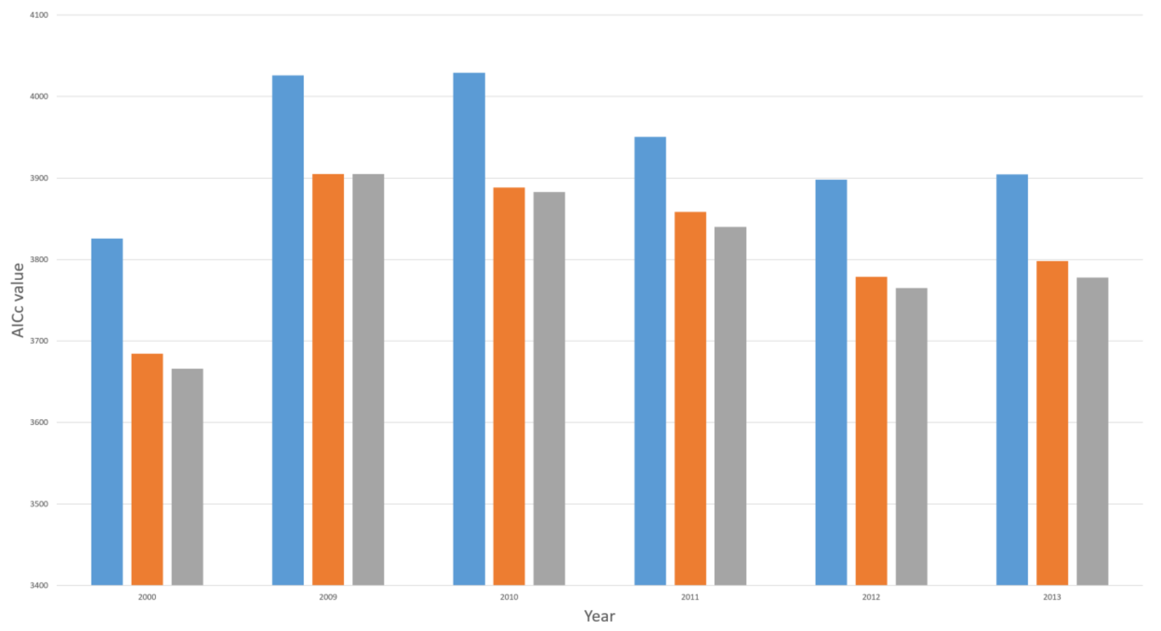
| AIC | 3825.92 | 4029.05 | 4025.85 | 3950.59 | 3897.81 | 3904.38 |
| Adjusted R2 | 0.71 | 0.73 | 0.64 | 0.65 | 0.67 | 0.66 |
| Decennial Census Years | ACS Years | |||||
|---|---|---|---|---|---|---|
| Year | 2000 | 2010 | 2009 | 2011 | 2012 | 2013 |
| Bandwidth | 84 | 98 | 98 | 91 | 77 | 90 |
| RSS | 531,883.1 | 111,8276 | 1,166,110 | 951,077.8 | 633,734.2 | 786,608.1 |
| AIC | 3684.43 | 3888.25 | 3904.78 | 3858.53 | 3778.99 | 3798.11 |
| Adjusted R2 | 0.86 | 0.81 | 0.80 | 0.79 | 0.84 | 0.81 |
| Decennial Census Years | ACS Years | |||||
|---|---|---|---|---|---|---|
| Year | 2000 | 2010 | 2009 | 2011 | 2012 | 2013 |
| Bandwidth | 84 | 98 | 98 | 84 | 77 | 90 |
| RSS | 635,797 | 1,402,213 | 1,479,242 | 1,188,077 | 944,864 | 922,170 |
| AIC | 3666 | 3883 | 3905 | 3840 | 3765 | 3778 |
© 2018 by the authors. Licensee MDPI, Basel, Switzerland. This article is an open access article distributed under the terms and conditions of the Creative Commons Attribution (CC BY) license (http://creativecommons.org/licenses/by/4.0/).
Share and Cite
Ma, Y.; Gopal, S. Geographically Weighted Regression Models in Estimating Median Home Prices in Towns of Massachusetts Based on an Urban Sustainability Framework. Sustainability 2018, 10, 1026. https://doi.org/10.3390/su10041026
Ma Y, Gopal S. Geographically Weighted Regression Models in Estimating Median Home Prices in Towns of Massachusetts Based on an Urban Sustainability Framework. Sustainability. 2018; 10(4):1026. https://doi.org/10.3390/su10041026
Chicago/Turabian StyleMa, Yaxiong, and Sucharita Gopal. 2018. "Geographically Weighted Regression Models in Estimating Median Home Prices in Towns of Massachusetts Based on an Urban Sustainability Framework" Sustainability 10, no. 4: 1026. https://doi.org/10.3390/su10041026
APA StyleMa, Y., & Gopal, S. (2018). Geographically Weighted Regression Models in Estimating Median Home Prices in Towns of Massachusetts Based on an Urban Sustainability Framework. Sustainability, 10(4), 1026. https://doi.org/10.3390/su10041026