Article

Scenarios Simulation of Spatio-Temporal Land Use Changes for Exploring Sustainable Management Strategies

1
College of Horticulture and Forestry Sciences/Hubei Engineering Technology Research Center for Forestry Information, Huazhong Agricultural University, Wuhan 430070, China
2
College of Resources and Environment, Huazhong Agricultural University, Wuhan 430070, China
*
Author to whom correspondence should be addressed.
Sustainability 2018, 10(4), 1013; https://doi.org/10.3390/su10041013
Submission received: 3 January 2018 / Revised: 9 March 2018 / Accepted: 26 March 2018 / Published: 29 March 2018

Abstract

:
Land use and land cover change have received considerable attention from global researchers in recent decades. The conflicts between different development strategies for land uses have become a problem that urgently needs to be solved, especially in those regions with a fragile ecological environment. The development of scenario simulations is essential in order to highlight possible alternative pathways for the future under the backgrounds of urbanization, economic growth and ecological protection. This study simulated land use changes for Tekes in 2020 with the Conversion of Land Use and its Effects at Small regional extent (CLUE-S) model under a ‘business as usual’ scenario, cropland protection scenario, ecological security scenario, and artificial modification scenario. The results indicated that the spatial patterns of the land use types were explained well by the environment variables, and the selected models had a satisfactory accuracy in this study. The requirements and the patterns were quite different owing to the variation of the major objectives of the four scenarios. In addition to the constraint rules of the land use transformation, the hot point for land use change was its spatial coherency. Areas near to an existing land use type were more likely to transform to that type than those farther away. The increased cropland and urban land were mainly located around the current cropland and urban land while forests and grassland were more likely to occur in places with flat terrain and good hydrological conditions. The results could contribute to better insight into the relationships between land use changes and their driving factors and provide a scientific basis for regional management strategies and sustainable land use development.

1. Introduction

Land use changes could bring a number of environmental and ecological problems, such as decrease in biodiversity [1], resource depletion, and the degradation of ecosystem services [2]. There are irreconcilable conflicts between urban development and agricultural land preservation, which are becoming increasing contentious in China [3,4]. The government of China has adopted many strategic policies such as “Building New Countryside” and “Implementing New-Type Urbanization” in the context of rapid economic development to promote such development [5,6]. To prevent the decline in cropland, the “arable land requisition-compensation balance” policy was proposed in 1997, which was a strict cropland protection policy in China [7]. On the other side, the policies of “Natural Forest Protection” and “Grain for Green” are introduced in 1998 and 1999 to assist in the protection of the ecological environment. Rapid urbanization has promoted social and economic development and benefits the people in terms of income growth and improved living conditions [8]. The urban population in China reached 50% for the first time in 2011 [9,10]. The conflicts under different development strategies has become a problem that urgently needs to be solved, especially in northwestern China, which has a vulnerable ecological environment. The land uses are highly sensitive to human activities in such regions. Mining, farming, and timber harvesting have changed the land uses [11]. A large amount of cropland is unstable due to poor soil and water conditions. The process of developing land and water resources leads to the degradation of primitive forest, which is transformed into artificial woodland or construction land [12]. As the harmonic development of the socio-economic and ecological environment is the main theme of current society, how to solve these conflicts properly becomes an important issue.
Simulating and modelling dynamic processes are important in the correlative fields, such as farmland abandonment [13], urban expansion [14] and land-use management [15]. Predicting land use changes can assist in determining the extent of degradation and enabling the managers to control changes in the proper directions [16,17,18]. From a planning and management perspective, it is of great significance to have an explicit understanding of predicted land use change as well as the underlying drivers [19,20,21]. The processes and mechanisms of land use change are complex and largely influenced by natural and socio-economic driving factors [22]. Brandt et al. (1999) classified the driving variables of land use change into more specific categories including natural, socio-economic, political, technological, and cultural [23]. Population growth generates increased demands for resources and construction land [24]. Thus, human disturbances such as pollution, fire, grazing, cutting, and cultivation can also lead to spatial shifts in land use systems [25,26]. Natural disasters, such as hurricanes, are threats to the land uses and can cause substantial damage [27]. The relative influence of the driving factors varied from region to region [28]. The geographic position and the social background should therefore be considered when exploring the drivers of land use changes for a given area.
Fully understanding the change processes of land use types with different speeds is still a challenging issue [29]. Model-assisted planning has become a useful tool for decision-makers to explore complexity and uncertainty and develop solutions for active engagement with an uncertain condition [30]. Over the last few decades, a variety of land use and land cover change models have been utilized in land management and to better explore, project and assess the effect of land use changes on the earth system in the future [31]. Previous models can be divided into two classes, including the statistical models and the spatially explicit models. The statistical models, such as regression models, Markov chains [32] and system dynamics (SD) [33] models, carry out statistical analysis on the driving variables on the basis of mathematical equations [34]. The spatially explicit models such as cellular automata (CA) [35], dynamics of land system (DLS) [36], CLUE-S [37] and agent-based [22] models, have the ability to allocate the spatial patterns of future changes [34].
How to choose an appropriate model in the prediction of land use change is an important issue. Each model has its own advantages and limits. The statistical models could not reveal the spatial pattern of land use changes. The CA model can simulate spatial and temporal land use dynamics and can be easily implemented [38] but the rules cannot be modified during the simulation [39] and it also could not capture interactions between socio-economic drivers and different areas [38]. The agent-based models performed well in simulating social processes by individual agents; however, most of these models can only predict simplified land uses due to the large number of interacting agents that need to be considered [40]. The combination of different models has been recently applied [34,41,42] and can make use of the specific strengths and overcome the weaknesses.
The CLUE-S model is an empirically based statistical and spatially explicit model and could deal with the competition between different land use types on the basis of systems theory. This model can better account for the processes of land use changes and the simulation result is objective and persuasive [41]. Besides, the CLUE-S model also has the ability to specify the details of the scenarios by the model parameters. Therefore, it has been widely and successfully applied in various fields, such as agricultural change [43], urban growth [41], and watershed land use dynamics [37]. However, the land use demands should be provided by a separate mathematical model for the CLUE-S model. The grey model (GM (1, 1)) is a time series forecasting model based on the grey system theory, which provides a method for exploring the relationships between the input and output processes with unclear inner relationships, uncertain mechanisms and insufficient information [44]. The combination of the CLUE-S model and the GM (1, 1) model could make full use of the advantages of these two models. Thus, a more realistic scenario simulation could be achieved to provide a scientific basis for exploring sustainable land use strategies.
Scenarios are widely applied in understanding land system change [45,46,47], exploring potential solutions for land use management [15], ecosystem services evaluation [47] and soil organic carbon analysis [48]. A stakeholder that makes qualitative storylines of the change direction is often involved in the process of scenario-building [49]. The storylines are constructed based on the existing conditions, which are regarded as feasible possibilities of the future [50]. The approaches of scenario setting have the ability to integrate different kinds of local knowledge [51]. The development of scenario simulations is essential in order to highlight possible alternative pathways for the future [52], such as the ecological security scenario or the cropland protection scenario for examining different strategies for how to create compromises between ecology health and economic benefits.
Tekes is located in an arid region of northwestern China. The ecological environment is vulnerable due to its special climate and topography conditions. The sea air is difficult to arrive due to the far distance from the ocean. It is arid with less rainfall compared to many other places. Over the past few decades, human activities, including urban sprawl, cropland transformation, grazing and timber harvesting, have created great stress on the environment. With the rapid development of the economy, local ecological security was threatened. Quantitative prediction of land use changes in different developmental directions is a most effective method for the government and decision-makers to resolve the problems between the environmental conservation and economic requirements.
The setting of conservation priority is the critical process of allocating the limited resources available for the conservation of the natural environment, biological diversity and ecosystem services [53]. However, introducing one kind or another of novel land management approaches to the already existing systems is a challenge for managers and the planners everywhere [52]. In this study, scenario simulations were performed in Tekes County by integrating the CLUE-S model and the GM (1, 1) model, which have extensive applications in other fields of research cases. The objectives of this paper are: (1) to predict requirements and finish the spatial allocations for different land use types with a combined model under four scenarios including the business as usual scenario, cropland protection scenario, ecological security scenario, and the artificial modification scenario at the county-scale; (2) to compare and discuss characteristics of spatially explicit land use distributions under different scenarios. The results could lead to insight into the relationships between land use changes and their driving factors under different constrained conditions in an arid region and could provide a scientific basis for the regulating and planning of land use.

2. Materials and Methods

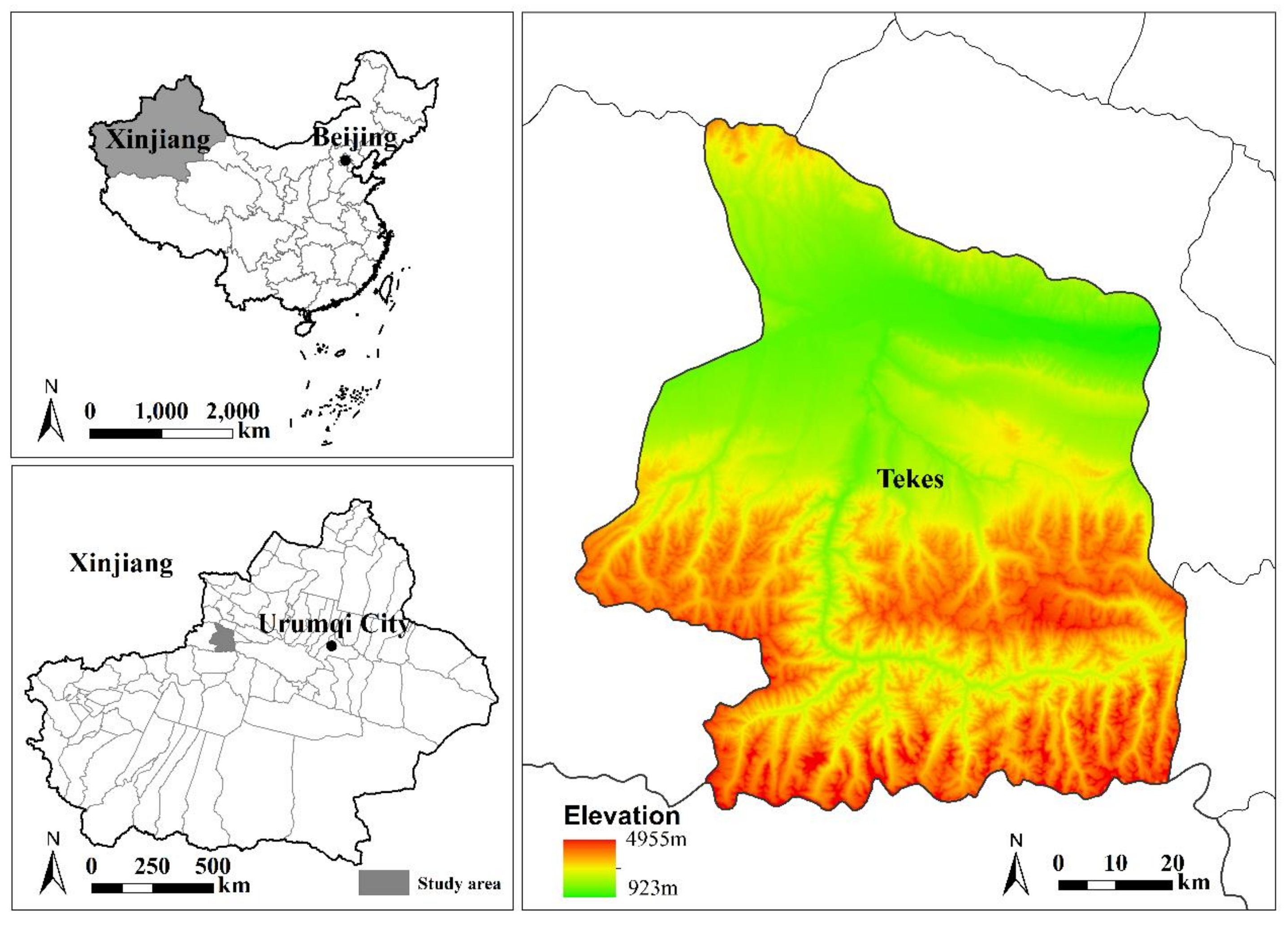
2.1. Description of the Study Area

Tekes is located in northwestern Xinjiang Province (latitude: 42°22′ and 43°25′ N, longitude: 81°19′ and 82°37′ E) in northwestern China. Tianshan Mountain lies in the south of Tekes County, the elevations of which range from 923 to 4955 m. The average annual rainfall and temperature are 383 mm and 5.3 °C, and the daily minimum and maximum temperatures are −32 °C and 33.5 °C, respectively. Three major rivers flow across the county and there are also three mountains stretching from west to east, which constitute about 94% of the whole area. The total population of Tekes was 148,600 in 1998 and 174,900 in 2015 [54,55]. Animal husbandry has developed well due to the rich pasture resources. There are large areas of unused land in Tekes, some of which are suitable to be reclaimed for agricultural land. However, the ecological environment is relatively fragile compared to other regions in the southeast of China. The simulation of land use changes is urgently needed for the harmonious development of ecology, the environment, and land use planning. Besides, the study area had undergone intensive land use changes in past years, resulting from complex natural and socio-economic factors, which made it an ideal area with which to perform scenario simulations. See Figure 1.

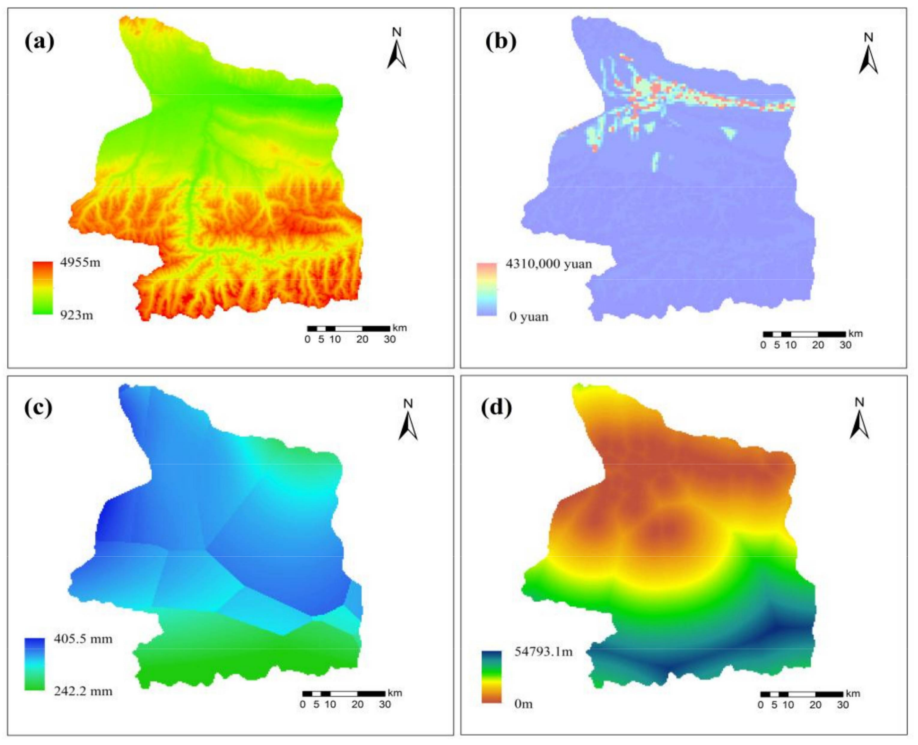
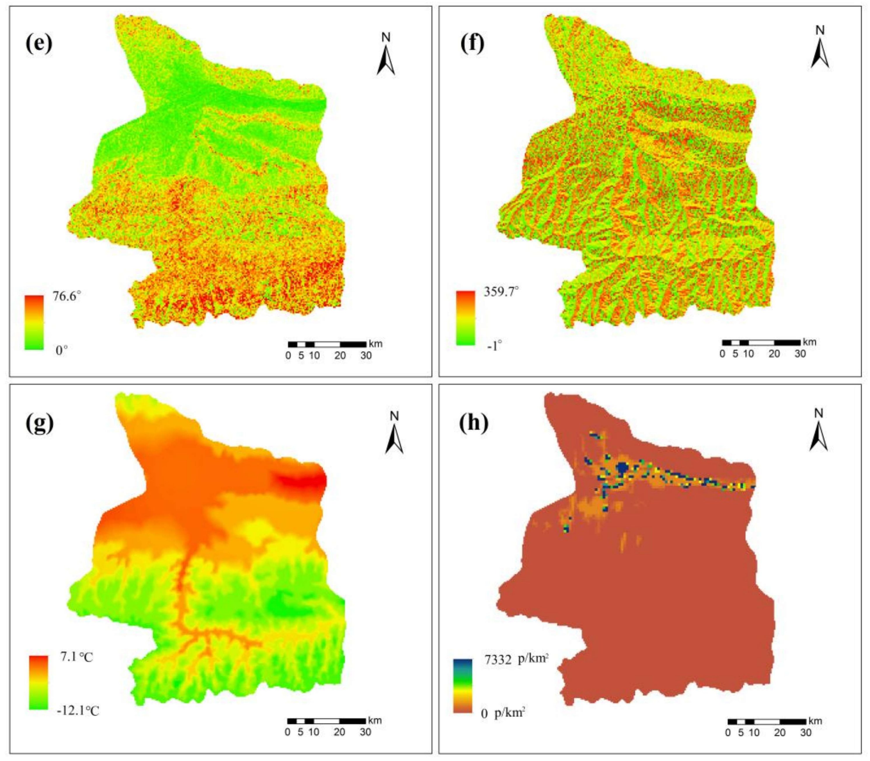
2.2. Data and Pre-Prosessing

The land use data of Tekes County was derived from Landsat TM images in 1998, 2006, and 2011 using supervised maximum likelihood classification in ERDAS. This part was on the basis of the work developed by Zhang et al. (2016) [56]. The landscapes were classified into six categories including forest, grassland, cropland, urban, barren land, and water. In this research, urban included single houses, settlements, industrial land and cities, and non-vegetated and sparsely vegetated areas were classified as barren land. A number of 300 validation plots were selected randomly in the study area in order to assess the accuracy of the classification and the observed landscape in these plots was visually identified based on the field data and high-resolution images from Google Earth [57]. The accuracy of the classification in this study can meet the requirements well with overall accuracies of 88.7%, 90.3%, and 93.7% for 1998, 2006, and 2011, and the corresponding kappa statistics were 0.86, 0.88, and 0.92 respectively.
Eight environmental variables, which were identified as the significant drivers of the patterns and the changes of the landscapes in Tekes [56], were used in this study to model the spatial patterns of the landscapes under different scenarios in 2020. The elevation, slope, and aspect were topography variables which were calculated from the digital elevation model (DEM). They were presented at the level of pixel units with a resolution of 30 m. The variable of distance to the nearest resident was calculated by using the distribution of residents, which was derived from the Landsat images of 2006. Socio-economic variables were derived from the database of natural resources of China, including the population density and the gross domestic product (GDP). Climate variables consisted of annual temperature and annual precipitation, which had the same origin as the socio-economic variables. The environmental variables selected for the simulation are described in Table 1.

2.3. Model Description

The scenario simulations of the landscape patterns of the study area in 2020 were conducted with the CLUE-S (the Conversion of Land Use and its Effects at Small regional extent) model and the GM (1, 1) model. This study was mainly focused on the amount of landscape changes as well as the spatial patterns in the future. The GM (1, 1) model is utilized to predict the requirements for each landscape without taking account of the spatial allocation.

2.3.1. CLUE-S Model

The CLUE-S model is used to predict the landscape change that has been validated by a wide range of applications [58]. As a developed version of CLUE, the CLUE-S model has the ability to display multiscale land use change, which was mostly applied in the research with a resolution between 20 and 1000 m [58,59]. The model has two distinct parts including the non-spatial demand module and the spatially explicit allocation module. The non-spatial module is an independent part of the model, which predicts the demand of each land use type resulting from the driving factors at the aggregate level. Scenarios and their specific applications should be considered in demand calculations, and the requirement of the land use types should be specified yearly, which is a direct input into the allocation module [60]. The land use requirements are allocated to individual grid cells in the spatial allocation module until the requirements have been satisfied with the rules based on a comprehensive and empirical analyses of the patterns of the current land use types [15,43].
The location suitability is established on the basis of an empirical analysis of the current and historic location preferences related to location characteristics, and is also based on the limited rules of a specific scenario [61]. The relative suitability of a place for each land use depends on the location characteristics [62]. Based on the results of location suitability, the CLUE-S model simulates the competition and interactions between different landscapes by using logistic regressions [31]. The logistic regression indicates the probability of each cell to be allocated to a land use type under the influences of a set of environmental variables following:
Log { P i / ( 1 P i ) } = β 0 + β 1 x 1 , i + β 2 x 2 , i + + β n x n , i
where Pi is the probability of a grid cell for the occurrence of the considered land use type and the x’s are the driving variables [60]. The relative probability of a particular land use at a particular place is decided by the natural and socioeconomic conditions [63,64]. The environmental variables considered as potential drivers were the eight significant variables of the patterns and the changes of the landscapes in Tekes described in Table 1. The spatial allocation of the land use types can be explained well by the environmental variables with high relative operating characteristic (ROC) values [65,66].

2.3.2. Scenarios Setting

Scenarios simulation was utilized to analyze the spatial pattern of the land use types in different constraint conditions, and the requirements of the land uses were input into the simulation models as the basic data. In this study, four scenarios were performed based on the backgrounds of the society, including a business as usual scenario, cropland protection scenario, ecological security scenario, and an artificial modification scenario.
In the scenario of business as usual, significant policies and regulations would not affect the amount and the pattern of the land use types. This scenario is characterized by disperse urban sprawl, inordinate cropland reclamation and abandonment. The areas and the spatial patterns of all the land uses would change on the basis of the trend from 1998 to 2011. The requirements of each land use during 1998 and 2020 were simulated using the GM (1, 1) model. As for the scenario of cropland protection, the cropland resources were limited to be transformed to other types in the simulation processes, on the other hand, other land uses could be changed to cropland. Transformations could occur among the rest of the types of land uses except cropland. The amount of cropland would increase under the restrict rules of this scenario, which can mitigate the stress of cropland shortage. In the scenario of ecological security, the environment of the target areas was protected in order to maintain the balance of the ecological environment and promote the sustainable development of the region. Large areas of forest, grassland and water, which play significant roles in ecosystem functions, are protected. The reclamation of ecological land uses would be restricted and land use transformations would occur only among cropland, urban land, and barren land. In the scenario of artificial modification, a large amount of barren land would be transformed into cropland besides the other types of land use transformation, including facility agriculture and being used as cropland directly. The requirements of cropland were the largest among the four scenarios, and the main land use transformation would occur in barren land and cropland. The development of facility agriculture could help increase the income of the people and promote the economy at the same time.

2.3.3. Requirements for the Land Use Types

Taking the year 1998 as the initial year and the year 2020 as the final year, the land use requirements of the land use types were simulated for Tekes between 1998 and 2020 at an annual time interval under the four scenarios. The requirements of the land use types of the cropland protection scenario, ecological security scenario, and artificial modification scenario in 2020 were predicted according to the characteristics of each scenario, and the land use demands during 1998 and 2020 were acquired by using the interpolation method. The GM (1, 1) model was conducted to predict the requirements of land use types in the scenario of business as usual. The grey system was introduced by Deng in 1982 [67], which is widely applied in engineering technology, economics, and land use management field [68]. The GM (1, 1) model, pronounced as “Grey Model First Order One Variable,” belongs to the keynote model of grey system theory and can predict the variation trend of data. The GM (1, 1) model could achieve effective predictions using a small sample size [69]. The GM (1, 1) model has the advantage of local optimization and the prediction accuracy is closely related to the selection of the initial condition [70]. The time series of the raw data from an unknown system may be random, however, the degree of randomness could be reduced by subjecting them to the accumulated generating operation (AGO) [71]. Then, the data would become a monotonic sequence and comply with the solution of the first order linear ordinary differential equation, so the solution curve could fit to the raw data with high precision [72]. The standard formula of the GM (1, 1) model is given as,
d x ( 1 ) / d t + a x ( 1 ) = u
The corresponding function on the time series of the standard formula is as follows,
x ( 1 ) = ( x ( 0 ) ( 1 ) u / a ) e a t + u / a
where x(0) is a non-negative sequence, x(1) is the following sequence, a is the developed coefficient and u is the grey action parameter, which can be established using the least-squares scheme in the Matlab software.

2.3.4. Model Configuration

A scenario test was performed before the land use prediction under resolutions from 100 m to 1000 m with a step of 100 m, and the optimal resolution was 500 m, which was the highest resolution that could make the model run successfully in this study. The CLUE-S model is based on a grid cell, which needs the land use data of the first year as the initial land use condition. In the stage of model validation, the land use in 2011 was predicted on the basis of the land use of 1998, in order to access the accuracy and applicability of the model. The simulated land use of 2011 was compared with the land use map of 2011 acquired from the supervised maximum likelihood classification from the Landsat TM images by using Kappa method [73]. The formula of Kappa coefficient is as follows,
K a p p a = ( P 0 P c ) / ( P p P c )
where P0 is the ratio of the number of correct simulation pixels and the total pixel number, Pc, is the expected value of the correct simulation, and Pp is the real accuracy of the land use classification. The Kstandard (standard kappa), Kno (alternative kappa), Klocation (location kappa), and Kquantity (quantity kappa) were calculated based on Kappa to evaluate the simulation. A detailed description of these parameters was developed by Pontius (2000) [74].
In the stage of scenario simulation, the land use data in 2011 was used as the initial land use condition to predict the spatial pattern in 2020 with the requirements of each land use types and other input files. Each land use including cropland, forest, grassland, urban, barren land, and water was encoded to 0–5, and the layer of the land use map was transformed to ASCII, which was the required form of the model.
A land use conversion matrix was constructed based on the regulation of land use transformation. As this study would predict the land use change in the near future, we supposed that urban could not be transformed to other land use types except water, while all the other land use types can convert to one another. There were two numbers in the matrix of the land use transformation, 0 represents that the land use could not be changed and 1 means that the corresponding land use can convert to other land use types. The land use transition rules are listed in Table 2. The conversion matrix in the four scenarios were the same while the restriction regions were different according to the characteristics of each scenario, which was marked by a separate value compared to the non-restriction regions.
The probabilities of transition for the land uses were different due to the costs and other specific conditions. The land use conversion elasticity was defined by the relative elasticity for change (ELAS) based on previous literature [41,42] and observed behavior in the recent past in the simulation models. The values of relative elasticity ranges from 0 to 1, which was based on the actual condition of the study area and the results of previous research. It would be more difficult for a land use to transform to any other land use types with a higher defined elasticity [60]. The ELAS parameters of the land use types are presented in Table 3. In this study, urban was the most difficult land use to transform to any other types with the ELAS parameter of 0.9, and barren land—the ELAS parameters of which was 0.5—was the easiest land use to transform to another type. As the restriction regions, which would be input into the simulation models with other parameters or data, were achieved based on the specific rules of the scenarios, all the scenarios used the same land use transition rules and ELAS parameters in this study. The variation of restriction regions and land use requirements played the major role in differentiating the results of the scenarios.

3. Results

3.1. Validation of the Model

Logistic regression coefficient, the corresponding ROC value, and the Pseudo R2 of each land use type are listed in Table 4. The results of the logistic regression indicate that the spatial pattern of all the six land use types could be explained well by the driving variables selected in this study.
In order to evaluate the accuracy of the CLUE-S model, the land use pattern of Tekes in 2011 based on the requirement of land use types was simulated. The land use demands during 1998 and 2011 were calculated by the method of interpolation depending on the actual land use data of 1998, 2006, and 2011. The requirements, together with the land use map of 1998, the layers of driving factors (see Figure 2), and other files of model parameters, were then inputted into the CLUE-S model to simulate the land use patterns for 2011.
The simulated and the actual land use map for 2011 are illustrated in Figure 3. The number of the pixels was 33,331 and the accurately simulated pixels was 27,001—as a result, the overall accuracy rate was 81.01% and the Kstandard, Kno, Klocation, and Kquantity for the validation result in 2011 were 0.7172, 0.7721, 0.7223, and 0.9903 respectively, indicating that this model had a high simulation ability in this study.

3.2. Land Use Demand in Different Scenarios

The results of the land use demand in the four scenarios are listed in Table 5 and Table 6. The residual test and posterior variance test were used to examine the results of the GM (1, 1) models, and the tests indicated that the GM (1, 1) models could presents satisfactory reliability in the simulations. In the business as usual scenario, each land use type would change in the same historical trend as during 1998 to 2011. Cropland and urban increased due to the increasing demand for food and population expansion. Grassland and forest increased with different rates, while barren land decreased a lot correspondingly.
In the scenario of cropland protection, the area of cropland increased under the restriction that cropland could not be transformed to other types. While for the artificial modification scenario, land use transformations could occur in cropland, there was additional cropland expansion due to the construction of facility agriculture. The grassland and forest were protected and continue to increase under different protection rules in the scenario of ecological security. The land use requirements for each scenario in 2020 are listed in Table 6.

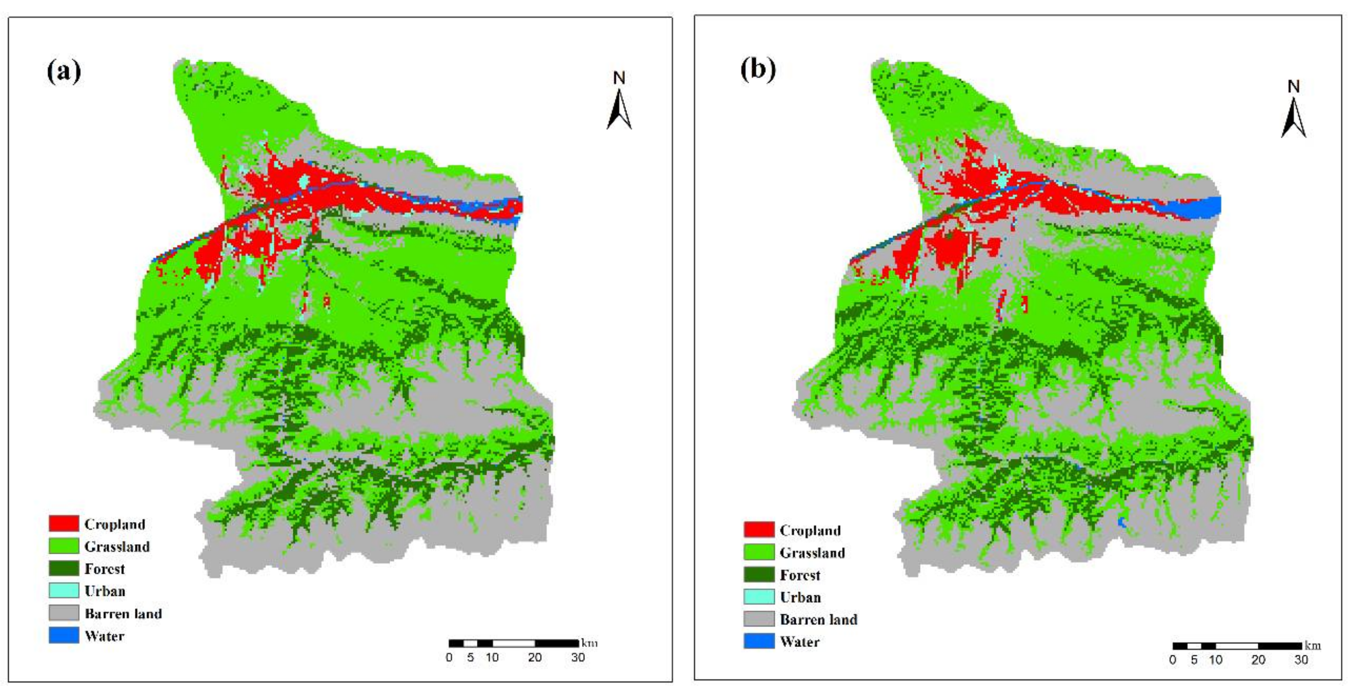
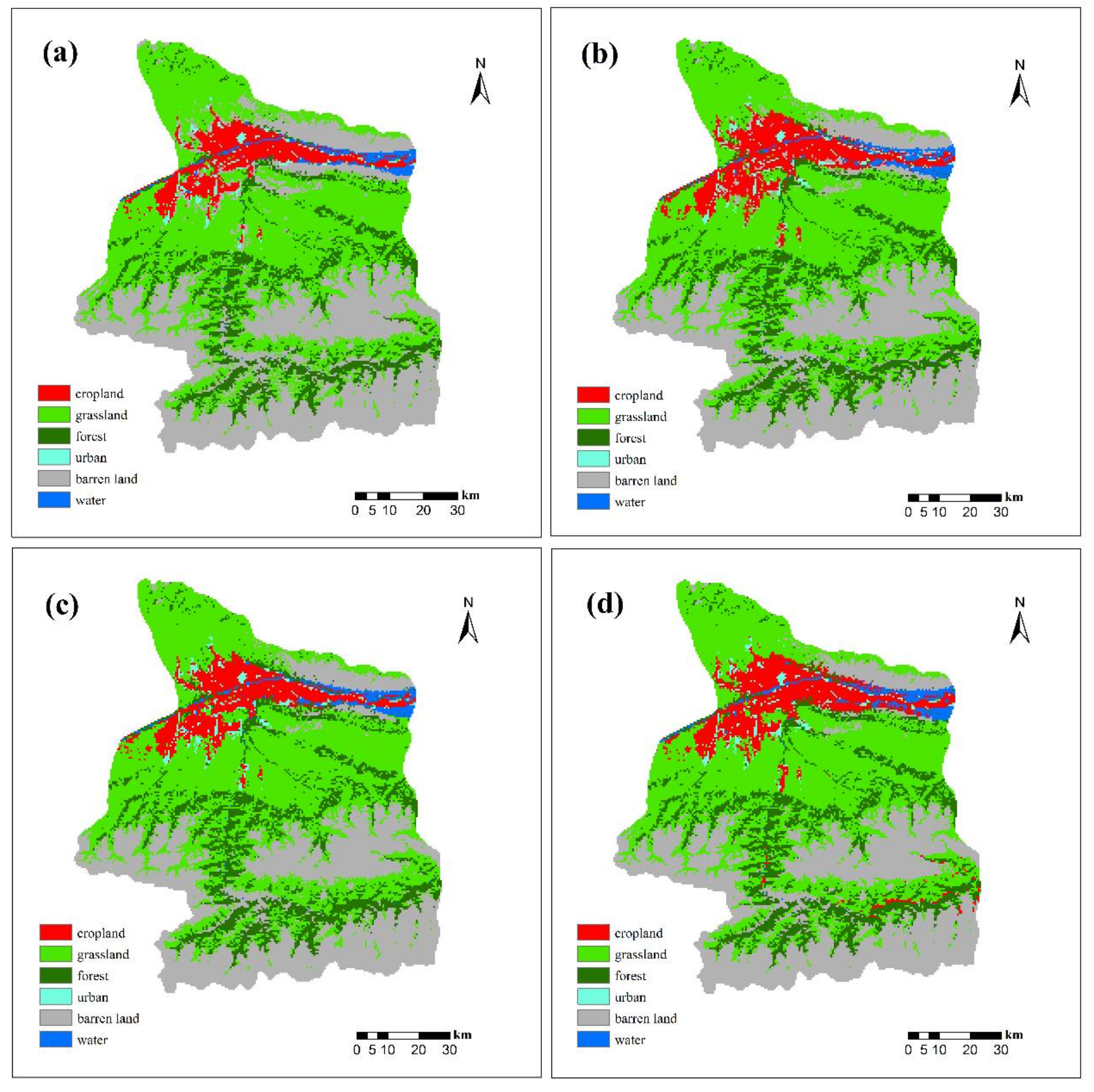
3.3. Spatial Simulation of Land Use in 2020

The spatial patterns of each land use type simulated for the four scenarios in 2020 are illustrated in Figure 4. As seen in the simulation results, the spatial patterns varied a lot, resulting from the restrict region and conversion rules, as well as the variation of the land use requirement. In the scenario of business as usual, urban sprawl mainly occurred near the original urban areas and the cropland. In the scenario of cropland protection, cropland increased around the existing cropland, which mainly came from barren land and partly from grassland. In the scenario of ecological security, the development was more concentrated around the barren land near to the urban land, providing an increase of forest and grassland. In the artificial modification scenario, the cropland increased dramatically towards the parts that were near to water and had a favorable topographic condition.

4. Discussion

4.1. Characteristics of Each Scenario Simulation

The CLUE-S model provides a comprehensive understanding of land use change processes and explores the spatial patterns of land use types in the future [62]. The application of the CLUE-S model could lead to a better understanding of land use changes, patterns and the underlying driving variables [15]. Thus, comprehensive land use strategies could be made based on the characteristics of the scenario simulations.
Cropland and grassland would continue to increase by 0.9% and 5.3% respectively during 2011 and 2020 under the business as usual scenario. With the expansion of the population and the development of society, the area of urban land would increase by 19.5% in 2020. Under the cropland protection scenario, the present cropland was protected and was prohibited from changing and other land use types could be transformed to cropland. The increase in forests and grassland were the main characteristics under the ecological security scenario. Large areas of barren land would be reclaimed to cropland in order to gain more economic benefits during 2011 and 2020 under the artificial modification scenario.
As for the scenario of business as usual, urban land was expanding, and the increased urban land was mainly located around the original urban land and around the cropland. The increased grassland, which was mainly transformed from barren land, mostly occurred near the urban land. The forest was decreasing under the influence of the human activities, especially those next to the settlement places.
An increase in cropland and a decrease in barren land were the typical characteristics of land use changes under the cropland protection scenario. Cropland is mostly distributed in the surroundings of nearby settlements and water sources to facilitate farming [15]. Most of the cultivated fields were expanding around the existed cropland and or around the settlements, and the increased cropland was mainly transformed from barren land and grassland.
The expansion of forest and grassland was the main change under the ecological security scenario. Ecological land was prohibited from transforming into other land use types in order to protect the ecological environment and promote the harmonious development of the society, the economy and the environment. Most of the increasing ecological land was owed to the expansion of the existing forest and grassland through the transformation of the surrounding barren land. The barren land with a flatter terrain and better hydrological conditions was more easily transformed into ecological land. Ecological qualities are heterogeneous among different regions [42], so reasonable policies could be made according to regional variation of the ecological land dynamics.
Under the artificial modification scenario, the increased cropland was mainly transformed form barren land by the construction of the facility agricultural. Flat and accessible areas are preferred for agricultural use [21], so the added cropland was concentrated around the surrounding cropland and the residential land with flat topography and convenient traffic conditions. The increased arable land also occurred in the southern part of Tekes County with suitable natural and socio-economic conditions for modern agriculture.

4.2. Dissemination of Scenario Consequences

The scenario consequences are useful tools and had some potential options for the management of the environment and sustainable land use planning [75], which displayed the spatio-temporal patterns of land use changes under different environmental conservation strategies and socioeconomic backgrounds. The results could reflect the influences of land use change on the environment. For example, the expansion of agricultural land would potentially cause water scarcity and soil acidification [76]. The conversions from forestland and grassland to cropland would increase the soil erosion risk [33]. Accelerating urbanization could lead to the loss of urban green areas, the decline of biodiversity [35], resource depletion and a series of environmental and ecological problems and disasters [77].
The contradiction between economic development and environmental security is obvious in northwestern China. The continuous development of the economy would amplify the negative effects on the ecological environment. There were large areas of barren land such as the Gobi Desert, the proluvial fans and exposed soils, some of which were suitable for the residents to be reclaimed as cropland for economic benefits. On the other hand, efforts should be made when the ecological environment was threatened by the overuse of the land use types. However, it remains a challenge to selecting spatially effective ways to regulate the land use in relation to the existing land use types [15]. The scenarios designed in this study could help the decision makers overcome some of the challenges that might arise in land use management. Generally, the locations of the existing land use type were the suitable places for them, especially for the urban and cropland. The results of the scenario simulation also indicated that the expansion of the urban was mainly located in the areas near the original urban with flat terrain, convenient water and traffic conditions. Most of the increased cropland would occupy the barren land near the current cropland, which had more advantageous conditions for farmers to gain economic benefits. Given the characteristics of the land use changes obtained from the results of different scenario simulations, the government should pay more attention to agricultural production and ecological protection strategies to promote regional sustainable development.

4.3. Availability of the Integrated Method

It is obvious that no single model could obtain the main processes to identify land use change and to make an overall evaluation of environmental variables and the influences [62]. Each simulation model has advantages as well as constraints; as a result, the combination of different models becomes an advisable method. The integration of the CLUE-S model with the grey system theory model was used in this study to simulate land use change under different scenarios. The CLUE-S model could not project the land use demands with the consideration of the historical trends of the land use types; however, the GM (1, 1) model can overcome this issue. The CLUE methodology could allocate the requirements of each land use type at a regional scale on the basis of driving factors, land use transformation rules, and spatial restrictions to satisfy the balance between land use supply and requirement [37].
The validity of the simulation model is often assessed by comparing the accuracy of the model and a no-change model [78]. In this study, the actual land use data was regarded as the no-change model, the accuracy of this simulation model was validated through Kappa index and the percent ratio of the correctly simulated pixels. The results of the selected indexes denoted that the CLUE-S model combined with the GM (1, 1) model was an effective tool for exploring the characteristics of land use dynamics. The methods used in this study illustrated the spatial patterns of land use change in the future under different scenarios, which could help to reflect the complexity and to capture the main processes of the land use changes. According to the results of the model simulation, it was easy to detect the hot spots of the land use change, which indicated that the models used in this study could provide a scientific basis for land use management and decision-making.

5. Conclusions

The process of land use change is complex, and is caused by a series of natural and socio-economic variables. Accurate simulations for the near future are essential and of great significance. This study integrated multiple approaches and disciplinary models into the simulation processes of land use changes, which enabled us to better understand much more detailed storylines, land use patterns, and their relationships with the driving variables.
The requirements and the patterns of the land use types in 2020 were predicted under four different scenarios, which had its own constraint conditions and transformation rules for the land uses. The demands and the patterns of the land uses varied a lot among different scenarios. In addition to the constraint rules of land use transformation, the hot point for land use change had spatial coherency. The spatial allocation for the scenario simulation corresponded with some regularly observed phenomena that areas near to an existing land use type were more easily converted to that type than those areas farther away [32,33]. The increased cropland and urban land were mainly located around the original cropland and urban land. Forests and grassland were more likely to appear in places with flat terrain, convenient traffic and good hydrological conditions.
The land use patterns of the implementation of different planning strategies can be clearly visualized with the scenario simulation. From the scenarios, we can conclude that unused land with a high suitability for agriculture could be utilized for greenhouses or cropland to promote the economic development of the region. Appropriate ecological measures could also be established depending upon the scenario of ecological security. The conversions between cropland and unused land were common due to poor soil and water conditions. In order to maintain the cropland, protective measures for unstable cropland should be taken based on the simulated spatial patterns of cropland. The results could help to accomplish the goal of harmonious development between economic growth and ecological security under the background of urbanization and ecological degradation. The scenario prediction would be utilized as forecasting tools for regional governments and decision-making departments to assess the land use changes for reasonable development strategies as well as controlling the directions of the land use changes according to the characteristics of the simulation results. The CLUE-S model is a spatially explicit model and has been widely and successfully applied in various regions around the world. The GM (1, 1) model could simulate land use demands with insufficient information. Therefore, the combination of these two models could be applied in other regions and research fields easily. As the scenarios were designed based on the characteristics of the study area, the results of this paper could also provide a scientific basis for those areas that have similar fragile ecological environments and developing conflicts.

Acknowledgments

Financial support for this research was provided by the National Key Research and Development Program of China (no. 2017YFC0505401), and the Fundamental Research Funds for the Central Universities (no. 2662017QD002).

Author Contributions

Yu Zhang and Tianwei Wang designed the experiments and wrote the paper. Tianwei Wang participated in field survey. Yu Zhang performed the experiments. Pengcheng Wang and Chongfa Cai contributed to the analysis of the results. Zhaoxia Li and Mingjun Teng contributed to the scenario simulation. Tianwei Wang, Yu Zhang, and Zhaoxia Li revised the manuscript.

Conflicts of Interest

The authors declare no conflict of interests.

References

  1. Maeda, E.E.; De Almeida, C.M.; De Carvalho Ximenes, A.; Formaggio, A.R.; Shimabukuro, Y.E.; Pellikka, P. Dynamic modeling of forest conversion: Simulation of past and future scenarios of rural activities expansion in the fringes of the Xingu National Park, Brazilian Amazon. Int. J. Appl. Earth Obs. Geoinf. 2011, 13, 435–446. [Google Scholar] [CrossRef]
  2. Bürgi, M.; Silbernagel, J.; Wu, J.; Kienast, F. Linking ecosystem services with landscape history. Landsc. Ecol. 2015, 30, 11–20. [Google Scholar] [CrossRef]
  3. Han, J.; Hayashi, Y.; Cao, X.; Imura, H. Evaluating land-use change in rapidly urbanizing China: Case study of shanghai. J. Urban Plan. Dev. 2009, 135, 166–171. [Google Scholar] [CrossRef]
  4. Wang, X.H.; Yu, S.; Huang, G.H. Land allocation based on integrated GIS-optimization modelling at a watershed level. Landsc. Urban Plan. 2004, 66, 61–74. [Google Scholar] [CrossRef]
  5. Long, H.L.; Liu, Y.S.; Li, X.B.; Chen, Y.F. Building new countryside in China: A geographical perspective. Land Use Policy 2010, 27, 457–470. [Google Scholar] [CrossRef]
  6. Long, H.L.; Tu, S.S.; Ge, D.Z.; Li, T.T.; Liu, Y.S. The allocation and management of critical resources in rural China under restructuring: Problems and prospects. J. Rural Stud. 2016, 47, 392–412. [Google Scholar] [CrossRef]
  7. Lin, L.; Jia, H.Z.; Pan, Y.; Qiu, L.F.; Gan, M.Y.; Lu, S.G.; Deng, J.S.; Yu, Z.L.; Wang, K. Exploring the patterns and mechanisms of reclaimed arable land utilization under the requisition-compensation balance policy in Wenzhou, China. Sustainability 2018, 10, 75. [Google Scholar] [CrossRef]
  8. Wang, C.D.; Wang, Y.T.; Wang, R.Q.; Zheng, P.M. Modelling and evaluating land-use/land-cover change for urban planning and sustainability: A case study of Dongying city, China. J. Clean. Prod. 2018, 172, 1529–1534. [Google Scholar] [CrossRef]
  9. Tan, Y.; Xu, H.; Jiao, L.; Ochoa, J.J.; Shen, L. A study of best practices in promoting sustainable urbanization in China. J. Environ. Manag. 2017, 193, 8–18. [Google Scholar] [CrossRef] [PubMed]
  10. Zhang, C.; Lin, Y. Panel estimation for urbanization, energy consumption and CO2 emissions: A regional analysis in China. Energy Policy 2012, 49, 488–498. [Google Scholar] [CrossRef]
  11. Wu, Z.T.; Zhang, H.J.; Krause, G.M.; Cobb, N.S. Climate change and human activities: A case study in Xinjiang, China. Clim. Chang. 2010, 99, 457–472. [Google Scholar] [CrossRef]
  12. Feng, Y.X.; Luo, G.P.; Lu, L.; Zhou, D.C.; Han, Q.F.; Xu, W.Q.; Yin, C.Y.; Zhu, L.; Dai, L.; Li, Y.Z.; et al. Effects of land use change on landscape pattern of the Manas River watershed in Xinjiang, China. Environ. Earth Sci. 2011, 64, 2067–2077. [Google Scholar] [CrossRef]
  13. Xie, H.L.; Wang, P.; Yao, G.R. Exploring the dynamic mechanisms of farmland abandonment based on a spatially explicit economic model for environmental sustainability: A case study in Jiangxi Province, China. Sustainability 2014, 6, 1260–1282. [Google Scholar] [CrossRef]
  14. Liu, Y.L.; He, Q.S.; Tan, R.H.; Liu, Y.F.; Yin, C.H. Modelling different urban growth patterns based on the evolution of urban form: A case study from Huangpi, Central China. Appl. Geogr. 2016, 66, 109–118. [Google Scholar] [CrossRef]
  15. You, W.B.; Ji, Z.R.; Wu, L.Y.; Deng, X.P.; Huang, D.H.; Chen, B.R.; Yu, J.A.; He, D.J. Modelling changes in land use patterns and ecosystem services to explore a potential solution for meeting the management needs of a heritage site at the landscape level. Ecol. Indic. 2017, 73, 68–78. [Google Scholar] [CrossRef]
  16. Brown, D.G.; Pijanowski, B.C.; Duh, J.D. Modeling the relationships between land use and land cover on private lands in the upper Midwest, USA. J. Environ. Manag. 2000, 59, 247–263. [Google Scholar] [CrossRef]
  17. Jenerette, G.D.; Wu, J. Analysis and simulation of land-use change in the central Arizona-Phoenix region, USA. Landsc. Ecol. 2001, 16, 611–626. [Google Scholar] [CrossRef]
  18. Hathout, S. The use of GIS for monitoring and predicting urban growth in east and west St Paul, Winnipeg, Manitoba, Canada. J. Environ. Manag. 2002, 66, 229–238. [Google Scholar] [CrossRef]
  19. Fathizad, H.; Rostami, N.; Faramarzi, M. Detection and prediction of land cover changes using Markov chain model in semi-arid rangeland in western Iran. Environ. Monit. Assess. 2015, 187. [Google Scholar] [CrossRef] [PubMed]
  20. Etter, A.; McAlpine, C.; Wilson, K.; Phinn, S.; Possingham, H. Regional patterns of agricultural land use and deforestation in Colombia. Agric. Ecosyst. Environ. 2006, 114, 369–386. [Google Scholar] [CrossRef]
  21. Fondevilla, C.; Colomer, M.À.; Fillat, F.; Tappeiner, U. Using a new PDP modelling approach for land-use and land-cover change predictions: A case study in the Stubai Valley (Central Alps). Ecol. Model. 2016, 322, 101–114. [Google Scholar] [CrossRef]
  22. Xu, Q.L.; Yang, K.; Wang, G.L.; Yang, Y.L. Agent-based modeling and simulations of land-use and land-cover change according to ant colony optimization: A case study of the Erhai Lake Basin, China. Nat. Hazards 2015, 75, 95–118. [Google Scholar]
  23. Brandt, J.; Primdahl, J.; Reenberg, A. Rural land-use and dynamic forces—Analysis of ‘driving forces’ in space and time. In Land-use Changes and Their Environmental Impact in Rural Areas in Europe; Krönert, R., Baudry, J., Bowler, I.R., Reenberg, A., Eds.; UNESCO: Paris, France, 1999; pp. 81–102. [Google Scholar]
  24. Wu, Y.Z.; Peng, Y.; Zhang, X.L.; Skitmore, M.; Song, Y. Development priority zoning (DPZ)-led scenario simulation for regional land use change: The case of Suichang County, China. Habitat Int. 2012, 36, 268–277. [Google Scholar] [CrossRef] [Green Version]
  25. Paudel, S.; Yuan, F. Assessing landscape changes and dynamics using patch analysis and GIS modeling. Int. J. Appl. Earth Obs. Geoinf. 2012, 16, 66–76. [Google Scholar] [CrossRef]
  26. Tzanopoulos, J.; Vogiatzakis, I.N. Processes and patterns of landscape changeon a small Aegean island: The case of Sifnos, Greece. Landsc. Urban Plan. 2011, 99, 58–64. [Google Scholar] [CrossRef]
  27. Schweizer, P.E.; Matlack, G.R. Factors driving land use change and forest distribution on the coastal plain of Mississippi, USA. Landsc. Urban Plan. 2014, 121, 55–64. [Google Scholar] [CrossRef]
  28. Newman, M.E.; McLaren, K.P.; Wilson, B.S. Long-term socio-economic and spatial pattern drivers of land cover change in a Caribbean tropical moist forest, the Cockpit Country, Jamaica. Agric. Ecosyst. Environ. 2014, 186, 185–200. [Google Scholar] [CrossRef]
  29. Basse, R.M.; Omrani, H.; Charif, O.; Gerber, P.; Bódis, K. Land use changes modelling using advanced methods: Cellular automata and artificial neural networks. The spatial and explicit representation of land cover dynamics at the cross-border region scale. Appl. Geogr. 2014, 53, 160–171. [Google Scholar] [CrossRef]
  30. Greiner, R.; Puig, J.; Huchery, C.; Collier, N.; Garnett, S.T. Scenario modelling to support industry planning and decision making. Environ. Model. Softw. 2014, 55, 120–131. [Google Scholar] [CrossRef]
  31. Mas, J.F.; Kolb, M.; Paegelow, M.; Olmedo, M.T.C.; Houet, T. Inductive pattern-based land use/cover change models: A comparison of four software packages. Environ. Model. Softw. 2014, 51, 94–111. [Google Scholar] [CrossRef] [Green Version]
  32. Subedi, P.; Subedi, K.; Thapa, B. Application of a hybrid cellular automaton—Markov (CA-Markov) model in land-use change prediction: A case study of saddle creek drainage basin, Florida. Appl. Ecol. Environ. Sci. 2013, 1, 126–132. [Google Scholar] [CrossRef]
  33. Xu, X.M.; Du, Z.Q.; Zhang, H. Integrating the system dynamic and cellular automata models to predict land use and land cover change. Int. J. Appl. Earth Obs. Geoinf. 2016, 52, 568–579. [Google Scholar] [CrossRef]
  34. Han, H.R.; Yang, C.F.; Song, J.P. Scenario simulation and the prediction of land use and land cover change in Beijing, China. Sustainability 2015, 7, 4260–4279. [Google Scholar] [CrossRef]
  35. Fuglsang, M.; Műnier, B.; Hansen, H.S. Modelling land-use effects of future urbanization using cellular automata: An Eastern Danish case. Environ. Model. Softw. 2013, 50, 1–11. [Google Scholar] [CrossRef]
  36. Samie, A.; Deng, X.Z.; Jia, S.Q.; Chen, D.D. Scenario-based simulation on dynamics of land-use-land-cover change in Punjab Province, Pakistan. Sustanability 2017, 9. [Google Scholar] [CrossRef]
  37. Luo, G.P.; Yin, C.Y.; Chen, X.; Xu, W.Q.; Lu, L. Combining system dynamic model and CLUE-S model to improve land use scenario analyses at regional scale: A case study of Sanggong watershed in Xinjiang, China. Ecol. Complex. 2010, 7, 198–207. [Google Scholar] [CrossRef]
  38. Haase, D.; Haase, A.; Kabisch, N.; Kabisch, S.; Rink, D. Actors and factors in land-use simulation: The challenge of urban shrinkage. Environ. Model. Softw. 2012, 35, 92–103. [Google Scholar] [CrossRef]
  39. Theobald, D.M.; Gross, M.D. EML: A modeling environment for exploring landscape dynamics. Comput. Environ. Urban Syst. 1994, 18, 193–204. [Google Scholar] [CrossRef]
  40. Parker, D.C.; Manson, S.M.; Janssen, M.A.; Hoffmann, M.J.; Deadman, P. Multi-agent systems for the simulation of land-use and land-cover change: A review. Ann. Assoc. Am. Geogr. 2003, 93, 314–337. [Google Scholar] [CrossRef]
  41. Zhou, R.; Zhang, H.; Ye, X.Y.; Wang, X.J.; Su, H.L. The delimitation of urban growth boundaries using the CLUE-S land-use change model: Study on Xinzhuang Town, Changshu City, China. Sustainability 2016, 8, 1182. [Google Scholar] [CrossRef]
  42. Lu, Y.; Wang, X.R.; Xie, Y.J.; Li, K.; Xu, Y.Y. Integrating future land use scenarios to evaluate the spatio-temporal dynamics of landscape ecological security. Sustainability 2016, 8, 1242. [Google Scholar] [CrossRef]
  43. Britz, W.; Verburg, P.H.; Leip, A. Modelling of land cover and agricultural change in Europe: Combining the CLUE and CAPRI-Spat approaches. Agric. Ecosyst. Environ. 2011, 142, 40–50. [Google Scholar] [CrossRef]
  44. Trivedi, H.V.; Singh, J.K. Application of grey system theory in the development of a runoff prediction model. Biosyst. Eng. 2005, 92, 521–526. [Google Scholar] [CrossRef]
  45. Wang, H.; Li, X.B.; Long, H.L.; Qiao, Y.W.; Li, Y. Development and application of a simulation model for changes in land-use patterns under drought scenarios. Comput. Geosci. 2011, 37, 831–843. [Google Scholar] [CrossRef]
  46. Murray-Rust, D.; Rieser, V.; Robinson, D.T.; Miličič, V.; Rounsevell, M. Agent-based modelling of land use dynamics and residential quality of life for future scenarios. Environ. Model. Softw. 2013, 46, 75–89. [Google Scholar] [CrossRef]
  47. Liu, J.Y.; Li, J.; Qin, K.Y.; Zhou, Z.X.; Yang, X.N.; Li, T. Changes in land-uses and ecosystem services under multi-scenarios simulation. Sci. Total Environ. 2017, 586, 522–526. [Google Scholar] [CrossRef] [PubMed]
  48. Olaya-Abril, A.; Parras-Alcantara, L.; Lozano-Garcia, B.; Obregon-Romero, R. Soil organic carbon distribution in Mediterranean areas under a climate change scenario via multiple linear regression analysis. Sci. Total Environ. 2017, 592, 134–143. [Google Scholar] [CrossRef] [PubMed]
  49. Alcamo, J. Environmental Futures—The Practice of Environmental Scenario Analysis; Elsevier: Oxford, UK, 2009. [Google Scholar]
  50. Raskin, P.D. Global scenarios: Background review for the Millennium Ecosystems Assessment. Ecosystems 2005, 8, 133–142. [Google Scholar] [CrossRef]
  51. Swetnam, R.D.; Fisher, B.; Mbilinyi, B.P.; Munishi, P.K.T.; Willcock, S.; Ricketts, T.; Mwakalila, S.; Balmford, A.; Burgess, N.D.; Marshall, A.R.; et al. Mapping socio-economic scenarios of land cover change: A GIS method to enable ecosystem service modelling. J. Environ. Manag. 2011, 92, 563–574. [Google Scholar] [CrossRef] [PubMed]
  52. Cotter, M.; Berkhoff, K.; Gibreel, T.; Ghorbani, A.; Goblon, R.; Nuppenau, E.A.; Sauerborn, J. Designing a sustainable land use scenario based on a combination of ecological assessments and economic optimization. Ecol. Indic. 2014, 36, 779–787. [Google Scholar] [CrossRef]
  53. Zhang, L.W.; Fu, B.J.; Lű, Y.H.; Zeng, Y. Balancing multiple ecosystem services in conservation priority setting. Landsc. Ecol. 2015, 30, 535–546. [Google Scholar] [CrossRef]
  54. Xinjiang Province Statistical Bureau. Statistical Yearbook of Xinjiang Province 1999; Xinjiang Province Statistical Bureau: Xinjiang, China, 1999. [Google Scholar]
  55. Xinjiang Province Statistical Bureau. Statistical Yearbook of Xinjiang Province 2016; Xinjiang Province Statistical Bureau: Xinjiang Province, China, 2016. [Google Scholar]
  56. Zhang, Y.; Wang, T.W.; Cai, C.F.; Li, C.G.; Liu, Y.J.; Bao, Y.Z. Landscape pattern and transition under natural and anthropogenic disturbance in an arid region of northwestern China. Int. J. Appl. Earth Obs. Geoinf. 2016, 44, 1–10. [Google Scholar] [CrossRef]
  57. Brinkmann, K.; Schumacher, J.; Dittrich, A.; Kadaore, I.; Buerkert, A. Analysis of landscape transformation processes in and around four West African cities over the last 50 years. Landsc. Urban Plan. 2012, 105, 94–105. [Google Scholar] [CrossRef]
  58. Verburg, P.H.; Veldkamp, A. Projecting land use transitions at forest fringes in the Philippines at two spatial scales. Landsc. Ecol. 2004, 19, 77–98. [Google Scholar] [CrossRef]
  59. Overmars, K.P.; Verburg, P.H.; Veldkamp, A. Comparison of a deductive and an inductive approach to specify land suitability in a spatially explicit land use model. Land Use Policy 2007, 24, 584–599. [Google Scholar] [CrossRef]
  60. Verburg, P.H.; Soepboer, W.; Veldkamp, A.; Limpiada, R.; Espaldon, V. Modelling the spatial dynamics of regional land use: The CLUE-S model. Environ. Manag. 2002, 30, 391–405. [Google Scholar] [CrossRef] [PubMed]
  61. Verburg, P.H.; Eickhout, B.; van Meijl, H. A multi-scale, multi-model approach for analyzing the future dynamics of European land use. Ann. Reg. Sci. 2008, 42, 57–77. [Google Scholar] [CrossRef]
  62. Liu, M.L.; Hu, Y.M.; Chang, Y.; He, X.Y.; Zhang, W. Land use and land cover change analysis and prediction in the upper reaches of the Mingjiang River, China. Environ. Manag. 2009, 43, 899–907. [Google Scholar] [CrossRef] [PubMed]
  63. Lambin, E.F.; Turner, B.L.; Geist, J.S.; Agbola, S.B.; Angelsen, A.; Bruce, J.W.; Coomes, O.T.; Dirzo, R.; Fischer, G.; Folke, C.; et al. The causes of land-use and land-cover change: Moving beyond the myths. Glob. Environ. Chang. 2001, 11, 261–269. [Google Scholar] [CrossRef]
  64. Geist, H.J.; Lambin, E.F. Proximate causes and underlying driving forces of torpical deforestation. Bioscience 2002, 52, 43–50. [Google Scholar] [CrossRef]
  65. Pontius, J.R.G.; Schneider, L.C. Land-cover change model validation by an ROC method for Ipswich watershed, Massachusetts, USA. Agric. Ecosyst. Environ. 2001, 85, 239–248. [Google Scholar] [CrossRef]
  66. Swets, J.A. Measuring the accuracy of diagnostic systems. Science 1986, 240, 1285–1293. [Google Scholar] [CrossRef]
  67. Deng, J.L. Control problems of Grey system. Syst. Control Lett. 1982, 5, 288–294. [Google Scholar]
  68. Chen, Y.H.; Li, X.B.; Su, W.; Li, Y. Simulating the optimal land-use pattern in the farming-pastoral transitional zone of Northern China. Comput. Environ. Urban Syst. 2008, 32, 407–414. [Google Scholar] [CrossRef]
  69. Zhou, W.; He, J.M. Generalized GM (1, 1) model and its application in forecasting of fuel production. Appl. Math. Model. 2013, 37, 6234–6243. [Google Scholar] [CrossRef]
  70. Zhang, J.X.; Zhang, P.; Wu, X.L.; Zhou, Z.Y.; Yang, C. Illumination compensation in textile colour constancy, based on an improved least-squares support vector regression and an improved GM (1, 1) model of grey theory. Color. Technol. 2017, 133, 128–134. [Google Scholar] [CrossRef]
  71. Deng, J.L. Introduction to grey system theory. J. Grey Syst. 1989, 1, 1–24. [Google Scholar]
  72. Chen, C.I.; Huang, S.J. The necessary and sufficient condition for GM (1, 1) grey prediction model. Appl. Math. Comput. 2013, 219, 6152–6162. [Google Scholar] [CrossRef]
  73. Cohen, J.A. A coefficient of agreement for nominal scales. Educ. Phychol. Meas. 1960, 20, 37–46. [Google Scholar] [CrossRef]
  74. Pontius, R.G., Jr. Quantification error versus location error in comparison of categorical maps. Photogram. Eng. Remote. Sens. 2000, 66, 1011–1016. [Google Scholar]
  75. Liu, Z.F.; Verburg, P.H.; Wu, J.G.; He, C.Y. Understanding land system change through scenario-based simulations: A case study form the drylands in Northern China. Environ. Manag. 2017, 59, 440–454. [Google Scholar] [CrossRef] [PubMed]
  76. Li, J.W.; Liu, Z.F.; He, C.Y.; Tu, W.; Sun, Z.X. Are the drylands in northern China sustainable? A perspective from ecological footprint dynamics from 1990 to 2010. Sci. Total Environ. 2016, 553, 223–231. [Google Scholar] [CrossRef] [PubMed]
  77. Imhoff, M.L.; Bounoua, L.; DeFries, R.; Lawrence, W.T.; Stutzer, D.; Tucker, C.J. The consequences of urban land transformation on net primary productivity in the United States. Remote Sens. Environ. 2004, 89, 434–443. [Google Scholar] [CrossRef]
  78. Van Vliet, J.; Bregt, A.K.; Hagen-Zanker, A. Revisiting Kappa to account for change in the accuracy assessment of land-use change models. Ecol. Model. 2011, 222, 1367–1375. [Google Scholar] [CrossRef]
Figure 1. Location of the study area.
Sustainability 10 01013 g001
Figure 2. The driving factors of the land use simulation: (a) elevation; (b) Gross Domestic Product (GDP); (c) annual precipitation; (d) distance to the nearest resident; (e) slope; (f) aspect; (g) annual temperature; (h) population density.
Sustainability 10 01013 g002aSustainability 10 01013 g002b
Figure 3. Comparison between (a) the predicted land use map in 2011 and (b) the actual land use map in 2011 of Tekes.
Sustainability 10 01013 g003
Figure 4. Simulated land use maps for different scenarios of Tekes in 2020. (a) business as usual scenario; (b) cropland protection scenario; (c) ecological security scenario and (d) artificial modification scenario.
Sustainability 10 01013 g004
Table 1. Description of the environmental variables selected for the simulation model.
AbbreviationsDescriptionUnitSource of the Data
TemAnnual temperature°CDatabase of natural resources of China (cell size 500 m)
PreAnnual precipitationmmDatabase of natural resources of China (cell size 500 m)
EleElevationmDigital elevation model (cell size 30 m)
SlpSlope%Digital elevation model (cell size 30 m)
AspAspect°Digital elevation model (cell size 30 m)
PopPopulation densityp/km2Database of natural resources of China (2003, cell size 1000 m)
GDPGross domestic productyuanDatabase of natural resources of China (2003, cell size 1000 m)
DisDistance to the nearest residentmBase cartography of the study area (cell size 30 m)
Table 2. Land use transition rules.
Land Use CroplandGrasslandForestUrbanBarren LandWater
Cropland111111
Grassland111111
Forest111111
Urban000101
Barren land111111
Water111111
Table 3. Relative elasticity for change (ELAS) parameters of each land use types.
Land Use TypesCroplandGrasslandForestUrbanBarren LandWater
ELAS parameters0.80.70.80.90.50.8
Table 4. Logistic regression coefficient of each land use type for Tekes.
VariablesCroplandGrasslandForestUrbanBarren LandWater
Elev−0.0090 *0.0011 *−0.0037 *0.00270.0016 *−0.0036
GDP0.0066−0.0625 *−1.6022 *0.0022−0.01020.0156
Pre0.0102 *0.0014 *0.0024 *−0.0075−0.0028 *−0.0013
Dis−0.0004 *0.000010.0001 *−0.0026 **−0.0001 *0.0001
Slp−0.1378 *−0.0119 **0.0529 *−0.29170.00760.0235
Asp−0.0009−0.00090.0025 *0.00380.0006−0.0041
Temp0.02400.0256 *−0.0111−0.0574−0.01040.0068
Pop−0.0004−0.1087 *−0.0823 **0.0004−0.0114 *−0.0052
Constant−21.3680−7.5267−3.221121.74376.07013.6570
ROC0.9800.8560.9350.9390.8940.818
Pseudo R20.8930.4170.5090.3260.5110.138
Note: * and ** represent significance at 0.01 level and 0.05 level, respectively.
Table 5. Prediction of land use demand based on grey model (GM) (1, 1) model for the business as usual scenario.
YearCroplandGrasslandForestUrbanBarren LandWater
2012503.43389.31092.069.93183.2101.5
2013503.73408.11087.972.13165.2105.4
2014504.03427.01083.874.33147.2109.4
2015504.33446.01079.876.73129.4113.5
2016504.53465.21075.779.03111.7117.8
2017504.83484.41071.781.53094.0122.2
2018505.13503.71067.784.13076.5126.9
2019505.33503.71063.786.73059.1131.7
2020505.63523.21059.889.43041.7136.6
Table 6. Prediction of land use demands for 2020 in different scenarios.
ScenariosCroplandGrasslandForestUrbanBarren LandWater
2011504.33368.01151.069.53147.892.3
Business as usual505.63523.21059.889.43041.7136.6
Cropland protection666.23580.61124.199.92706.2149.9
Ecological security582.93663.81249.099.92589.7141.6
Artificial modification749.43580.61165.899.92589.7141.6

