Abstract
Improving green productivity is an important way to achieve sustainable development. In this paper, we use the Global Malmquist-Luenberger (GML) index to measure and decompose the green productivity growth of 18 cities in Xinjiang over 2000–2015. Furthermore, this study also explores factors influencing urban green productivity growth. Our results reveal that the urban green productivity in Xinjiang has slowly declined during the sample period. Technological progress is the main factor contributing to green productivity growth, while improvements in efficiency lag behind. Implementing stricter environmental regulation, improving infrastructure, and appropriately enhancing the spatial agglomeration of economic activities may improve green productivity, while the increase in the size of the industrial base in the near future will likely hinder green productivity growth. Based on these results, this paper puts forward corresponding policy suggestions for the sustainable development of the urban economy in Xinjiang.
1. Introduction
Since the economic and political reforms of 1978, when China began to open up to the outside world, China’s economy has made remarkable achievements and has become the second largest economy in the world. However, environmental pollution and resource consumption is increasingly becoming a serious problem for China, especially considering China’s rapid economic growth. According to a report from the International Institute of Low Carbon Economy, China consumes about 21% of the world’s energy, 11% of its oil, and 49% of its coal, resulting in China producing 26% of the world’s sulfur dioxide, 28% of its nitrogen oxides, and 25% of its carbon dioxide [1]. Environmental pollution has a serious impact on the economic development and human health. For example, air pollution has caused China to lose an estimated 10% of its GDP [2] as well as 350,000 to 500,000 premature deaths [3]. This extensive development mode, requiring high levels of inputs and high levels of pollution is not sustainable [4], and hinders the country from realizing further economic growth [5]. The key to sustainable growth for China’s economy is to improve production efficiency while reducing resource consumption and environmental pollution.
Xinjiang, China’s largest province, is located in the arid and semi-arid areas of the far west and is currently going through a period of rapid industrialization and urbanization. With rapid economic development, the negative impacts of water pollution, air pollution, desertification, and overall ecological destruction have become increasingly prominent, which have changed Xinjiang into one of the unhealthiest regions in China. Cities are the centers of economic activity in Xinjiang and are also suffering from a shortage of resources and environmental pollution problems. Transforming modes of traditional economic growth into modes of intensive growth centered on improving green productivity may help cope with environmental pressures. However, due to the externality of resources and environment, the results of traditional evaluation will distort the estimates of social welfare changes and economic performance and provide misleading policy suggestions. Therefore, it is necessary to make unbiased measures of urban green productivity—including environmental factors—to provide better suggestions for the sustainable development of cities.
2. Literature Review
Since Solow’s [6] groundbreaking work, national- and sectoral-level productivity have been measured by applying a variety of parametric and non-parametric methods [7,8,9,10]. However, traditional models cannot precisely evaluate the quality of economic development until undesirable outputs of economic activities are incorporated into the estimation process. Ignoring the negative effects of environmentally harmful by-products in economic development can distort assessments of social welfare and economic performance and may be misleading for policy recommendations [11]. Economic activities are often accompanied by industrial waste water, industrial waste gases, and other pollution emissions, all of which affect sustainable economic development. Therefore, to more objectively reflect the quality of economic development, it is necessary to measure green productivity by integrating environmental pollution into the traditional total factor productivity accounting framework.
Green productivity, as presented by the Asian Productivity Organization (APO), is a strategy that integrates productivity improvement and environmental protection to achieve economic growth [12]. Chung et al. [13] proposed a directional distance function and extended the Malmquist index to the Malmquist-Luenberger productivity index (ML index) to measure green productivity growth. Thereafter, many scholars have calculated green productivity growth by employing the ML index. Fare [14] measured green productivity in manufacturing by US state and found an average annual growth rate of 3.6 percent from 1974 to 1986. Jeon [15], Lindenberger [16], and Yörük [17] analyzed productivity growth in the OECD economies and decomposed indices into technology change and efficiency change. Kumar [18] estimated conventional and environmentally sensitive productivity growth for 41 countries from 1981 to 2007 and found Non Annex-I countries had lower productivity growth compared Annex-I countries. Zhang et al. [19] and Zhang et al. [20] evaluated China’s productivity growth including undesirable outputs by adopting the ML productivity index.
Calculating the cross-period directional distance function (DDF) of the ML index is not feasible using linear programming [19,21,22,23,24]. In order to address this shortcoming, Oh [21] constructed the Global Malmquist–Luenberger (GML) productivity index. The GML index replaces the ML index by incorporating a global production possibility set into the DDF [23,24,25]. In recent years the GML productivity index has been widely used to measure green productivity, especially in China. Ananda and Hampf [26] measured the productivity of the Australian urban water sector using the GML productivity index and found that the conventional Malmquist index overestimated productivity growth. Wang and Feng [27] analyzed the environmental productivity of 30 sample provinces in China from 2003 to 2011. Fan et al. [28] used the GML index to evaluate and decompose the total factor CO2 emission performance of 32 industrial sub-sectors in Shanghai (China). Wang and Shen [29] employed the GML index to measure Chinese industrial productivity including environmental factors. However, most studies use the GML index to calculate green productivity at the regional [27,30,31,32,33] or industry levels [28,34,35], and relatively few studies explore productivity growth including pollution emissions at the urban level [24].
For the limited literature we know, most researches on green productivity mainly focus on regional or industry level, few studies explore the dynamic change of green productivity and its determinants at the urban level. In this paper, we apply the GML productivity index which incorporates both desirable output (GDP) and undesirable outputs (wastewater and sulfur dioxide) to evaluate the green productivity growth of oasis cities in Xinjiang, and then decompose this growth into efficiency changes and technological changes. Based upon a certain standard, we identify six green innovation cities. We also discuss the determinants driving green productivity growth by the panel data method. These results fill the research gap of urban green productivity in underdeveloped areas and have important policy significance for promoting the sustainable development of cities.
3. Methodology and Data
3.1. Measure Method
3.1.1. The Directional Output Distance Function
In this paper, each city in Xinjiang is regarded as a production decision making unit (DMU), thus constructing a production frontier for each of the 18 cities. We suppose each city uses N input factors, , and produces M desired outputs, , and I undesired outputs, . The production possibility set is defined as
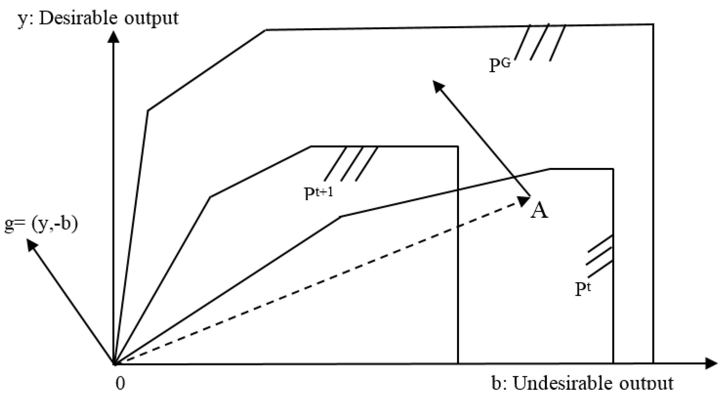
In order to better solve the problem of evaluating efficiency including “bad” (i.e., undesirable) outputs, we used the directional distance function introduced by Chung et al. [13]. This satisfies both the nature of the production possibility set and the direction of output expansion in the production process. The directional distance function based on output can be expressed using the following formula:
where represents the direction vector; indicates the value of DDF; and is the production set. To set the direction vector as weight, the DDF seeks to maximize the desired output (y) and minimize the undesired output (b). The relationship between the production feasibility set and the directional distance function is shown in Figure 1.
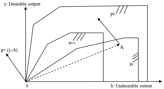
Figure 1.
The directional distance function that incorporates the desired outputs and the undesired outputs.
3.1.2. ML Productivity Index
Based on the DDF, Chung et al. [13] specified the ML productivity index, in which the ML index between times t and t + 1 is expressed as follows:
When ML index value is greater (lesser) than one, it indicates productivity growth (decline), implying production activity has produced more (less) desirable outputs and less (more) pollution.
3.1.3. GML Productivity Index
However, the ML index has a potential linear programming problem when measuring the cross-period DDF. In addition, the ML index expressed using the geometric mean is not circular or transitive. To remedy these weaknesses in the ML index, Oh [21] combined the Global Malmquist productivity concept with the directional distance function to formulate the GML index as an alternative.
A GML index value greater (less) than one represents productivity growth (decline) between period t and t + 1. As per Pastor and Lovell [25] and Oh [7], the GML index can be decomposed into two components: efficiency change (EC) and technical change (TC).
Here, is the efficiency change between periods t and t + 1, which evaluate the catching-up effect of a city toward the contemporaneous frontier, and an value greater (less) than one suggests green efficiency improvement (deterioration). represents the best practice gap between the contemporaneous technology frontier and the global technology frontier between periods t and t + 1, and a value greater (less) than one suggests green technical progress (regress).
3.2. Data and Variables
3.2.1. Data Collection
As of 2015, there are 26 cities in Xinjiang. Cities such as Horgos, Alashankou, Aral, Tumxuk, Wujiaqu, Beitun, Tiemenguan, and Shuanghe have relatively short histories, and their statistics data is lacking. Therefore, this paper excludes the above eight cities and selects the remaining 18 cities for sample analysis. The 18 sample cities (Urumqi, Changji, Fukang, Shihezi, Karamay, Kuitun, Bole, Yining, Tachen, Wusu, Aletai, Hami, Turpan, Akes, Korla, Kashi, Artux, and Hotan) account for 17 of Xinjiang’s land area, hold 40% of total population, and account for 70% of the Xinjiang’s gross domestic product (GDP) in 2015.
Considering the availability of data, this paper selects 18 cities in Xinjiang to measure green productivity over the period 2000–2015. The data are collected from the China City Statistical Yearbook, the Xinjiang Statistical Yearbook, and the Statistical Yearbooks of cities in Xinjiang.
3.2.2. Variable Selection
Based on the predecessor’s research, we choose capital stock and labor force as inputs and GDP as a desirable output. Given the air pollution and water pollution are the most serious pollution in Xinjiang, this study adopts industrial wastewater and industrial SO2 emissions to measure undesirable output. The details of input and output indicators are presented in Table 1. Capital stock is estimated by the perpetual inventory method using the formula: , where is the fixed capital stock, represents nominal fixed asset investment, is the fixed investment price index, and denotes the depreciation rate. The labor force is represented by the total number of urban employed persons at year-end.

Table 1.
Description of input and output variables.
The desirable output is expressed in terms of the annual GDP of the cities, and the GDP deflator is converted to the base period in 2000. The undesirable outputs are pollution emissions, including industrial wastewater and industrial sulfur dioxide.
The descriptive statistics of all input and output variables are shown in Table 2. The average value of capital stock for 18 cities is 45.27 billion RMB during the sample period. The average size of the labor force is 21 (ten thousand). The average real GDP value is 13.20 (billion RMB). The average emission levels of industrial sulfur dioxide and industrial wastewater are, respectively, 14.89 (thousand tons) and 10 (thousand tons).
Table 2.
A statistical description of input and output variables.
4. Empirical Results
4.1. Green Productivity Growth and Its Decomposition
The average (geometric mean) green productivity change of Xinjiang’s 18 cities in 2000–2015 is shown in Table 3. As shown, the average green productivity index is 0.986, indicating that green productivity fell by 1.4% in 2015 compared with that in 2000. In general, with the development of the urban economy in Xinjiang, the green productivity has not improved but has slowly declined, reflecting the fact that urban economic growth has followed the import-oriented extensive development model and not sustainable.
Table 3.
The growth of urban green productivity and its decomposition in Xinjiang (2000–2015).
The decomposition indices—namely the efficiency index and the technology index—are 0.985 and 1.005, respectively, implying that green efficiency fell by 1.5% and green technology improved by 0.5% over sample period. The average change in the rate of technological progress is more than 1, while the average efficiency change rate is less than 1 during sample period, suggesting that technological progress is main driving force of green productivity growth. The results show that cities in Xinjiang need to improve green efficiency and introduce advanced technologies.
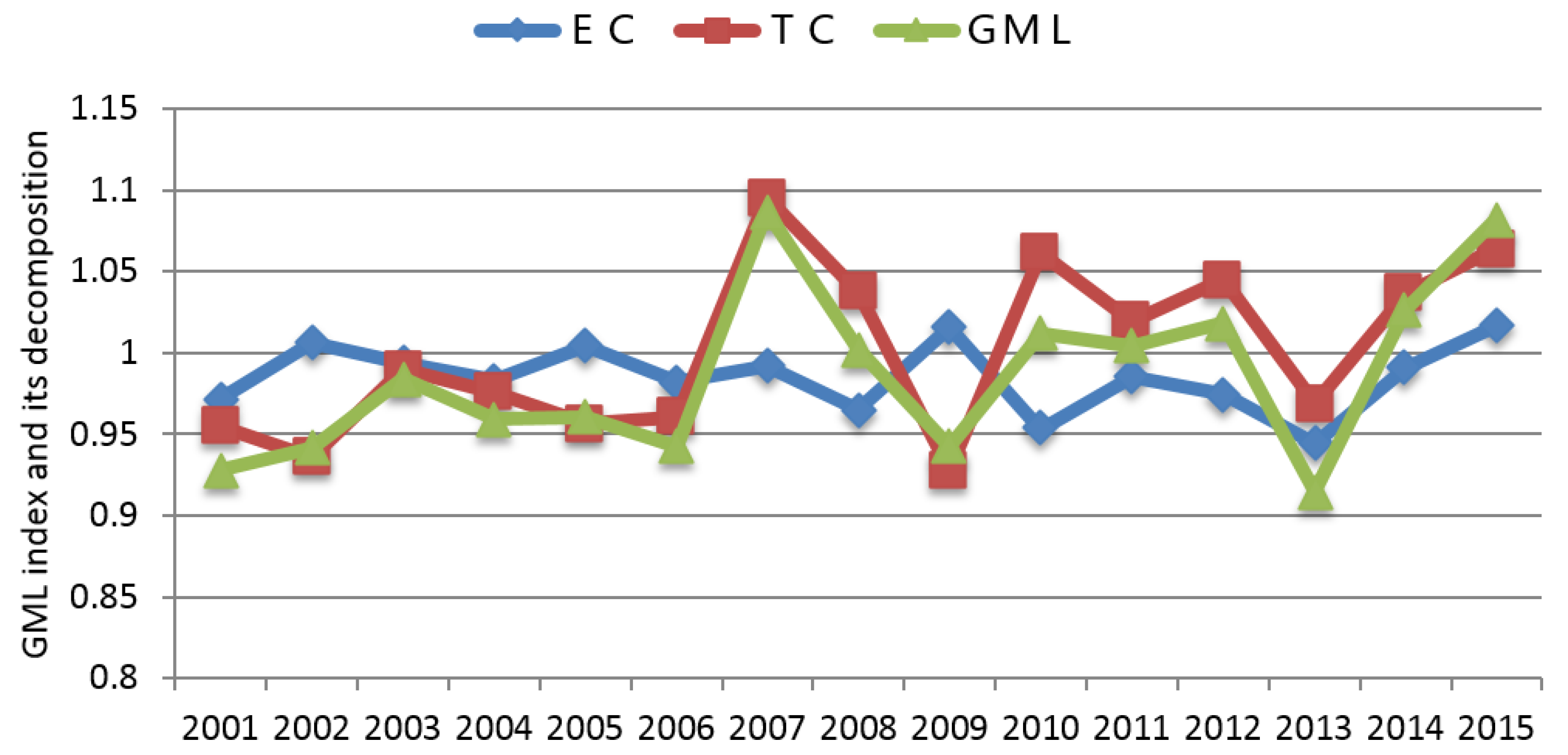
4.2. The Trend of Green Productivity Growth
As shown in Figure 2, the overall urban green productivity growth fluctuates around 1 and shows a trend of W running. It shows distinct and alternating phases of stability (2001–2006), rise (2007), decline (2008–2009), rise (2010–2012), decline (2013), and once again a rise (2014–2015). It is noteworthy that the green productivity growth rose most rapidly from 2001 to 2007. This was probably because the central government implemented a strategy of development of the western region and optimized the industrial sector by eliminating several high-pollution industries.
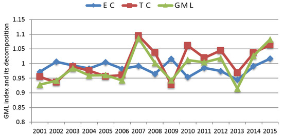
Figure 2.
Efficiency change, technological change, and green productivity growth trends of Xinjiang cities.
The green technology and green productivity indices showed similar trends for most of the period measured, with the exception of 2001, and both indices reached their highest level in 2007. The green efficiency index was somewhat less than green technology index for most of the period measured, a gap that may have hindered the growth of green productivity.
4.3. City Heterogeneity
As shown in Table 3, we found significant differences in the green productivity growth of the 18 cities. Only nine cities have a positive growth in green productivity, while other cities have negative growth in green productivity. Among these nine cities, Urumqi (1.063) and Korla (1.051) have the fastest green growth rates.
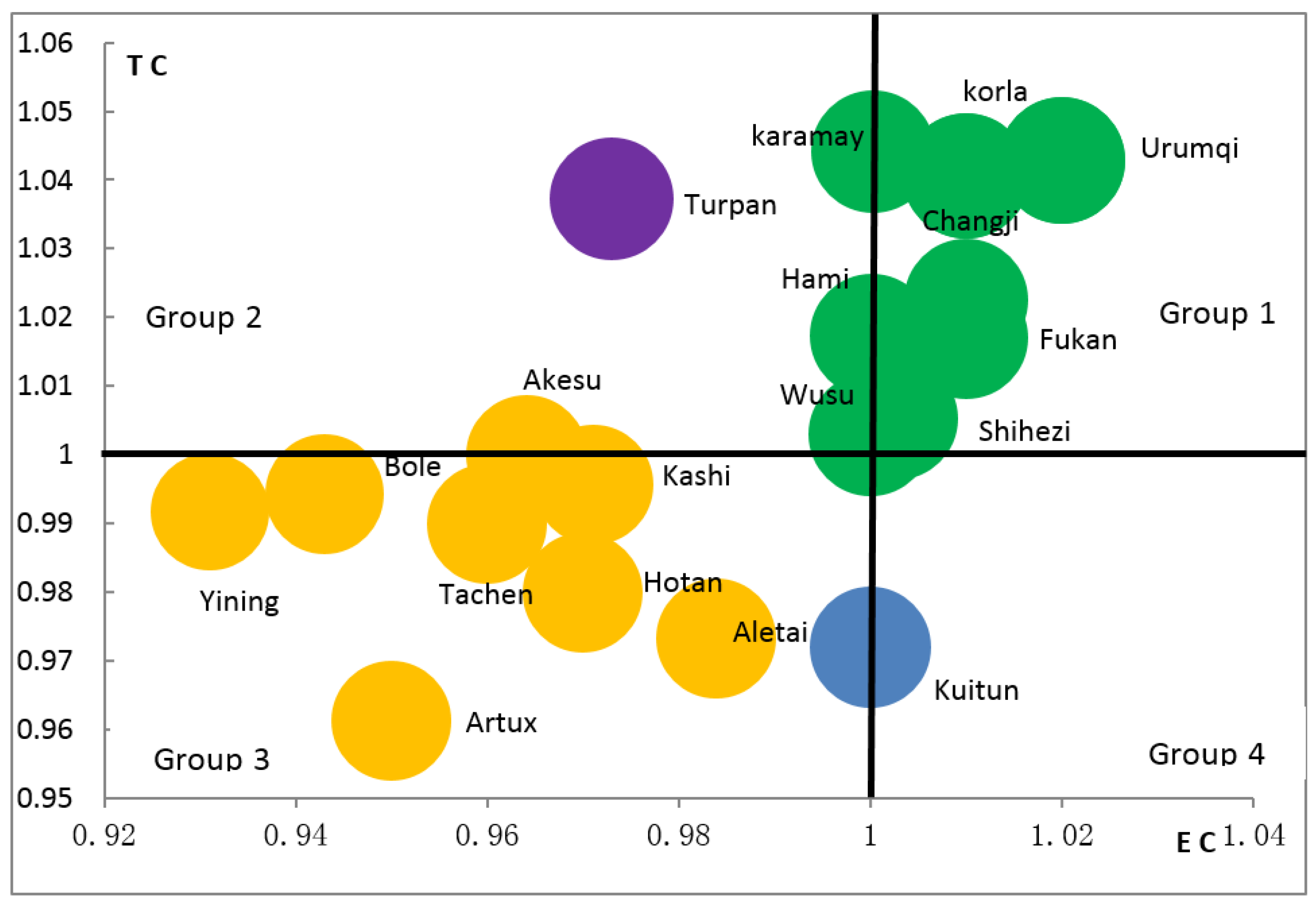
Figure 2 shows the heterogeneity of green productivity growth among cities in more detail. The X and Y axes of the figure represent the green efficiency index and the green technology index, respectively. The radius of the circle indicates mean green productivity growth. As per Oh and Heshmati [36], we divided the sample cities into different groups according to the green efficiency index and the green technology index. If the city green efficiency index was greater than 1, it is catching up with the production frontier. If the city green technology index is greater than the average, it has a (relatively) outstanding ability to innovate. According to the above criteria, we divided the 18 cities of Xinjiang into four groups (Figure 3).

Figure 3.
The green productivity change of various groups. The y-axis shows the green technology index, and the x-axis shows the green efficiency index. Note: The green, blue, purple, and yellow circles show groups 1, 2, 3, and 4 respectively.
Group 1 cities (TC ≥ 1.0006 and EC ≥ 1) are recognized as cities that are more innovative and farther along the catching-up process. These cities are catching up to the frontier and have shown a higher ability to innovate relative to other cities. These cities include Urumqi, Korla, Karamay, Shihezi, Fukang, Hami, Changji, and Wusu. Group 2 (TC ≥ 1.0006 and EC < 1) cities lag somewhat but are still relatively more innovative cities. Only Turpan is categorized in Group 2. Group 3 (TC < 1.0006 and EC < 1) cities both lag behind the catching-up process and are less innovative cities. Akes, Kashi, Bole, Tachen, Yining, Hotan, Aletai and Artux are in this group. Group 4 (TC < 1.0006 and EC ≥ 1) are catching up but less innovative cities. Kuitun is the only member of this group.
4.4. Regional Differences
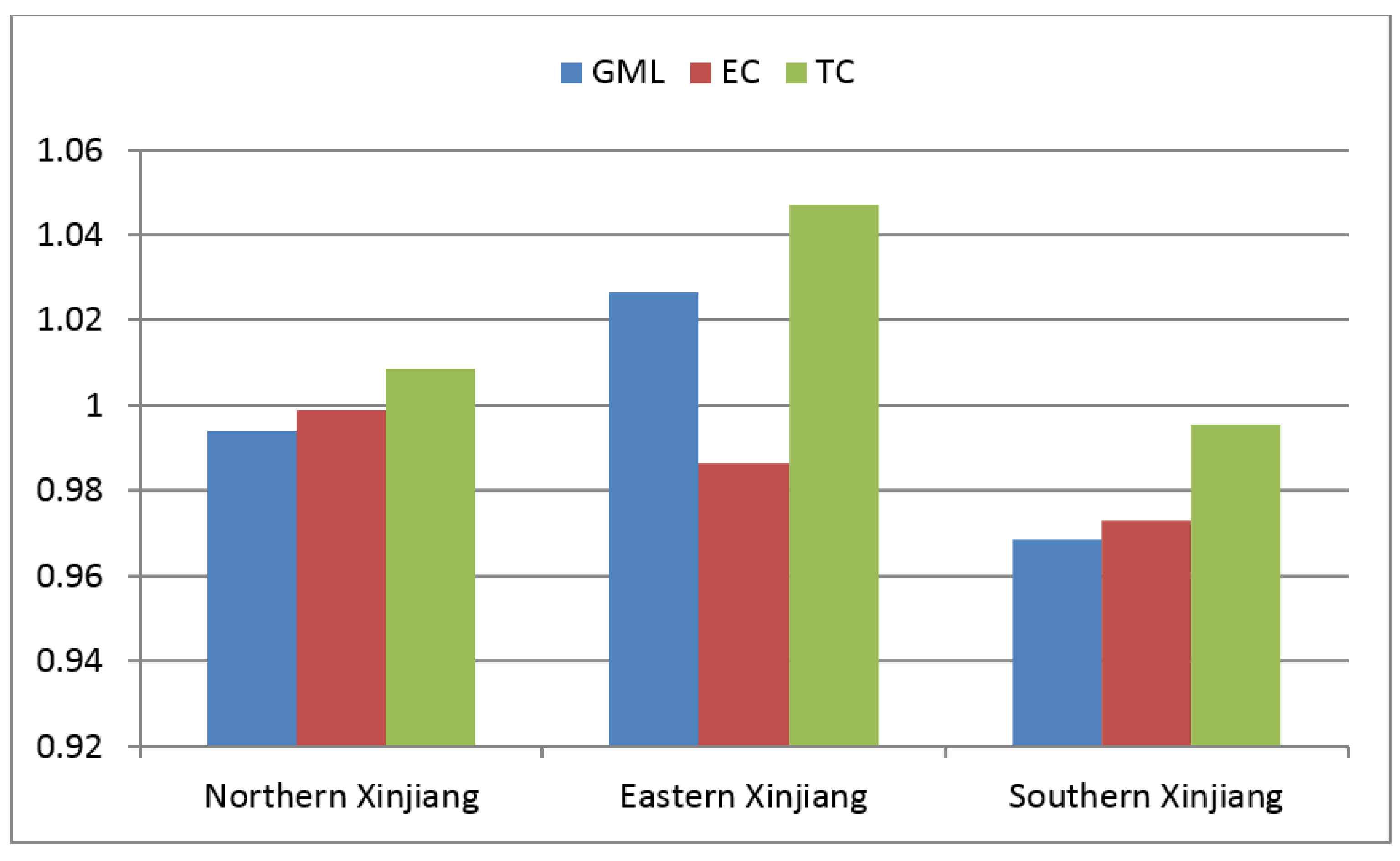
Based on their spatial distribution, the 18 cities in Xinjiang are divided into three groups: cities found in the North of the Xinjiang, cities found in the East of Xinjiang, and cities found in the South of Xinjiang. There are also some differences in urban green productivity growth between different regions (Figure 4). The green productivity growth of cities found in the East of Xinjiang is higher than that of other regions, which suggests that the region has improved green productivity by increasing the intensity of environmental pollution controls. In contrast, the green productivity growth of cities found in the North of Xinjiang and cities found in the South of Xinjiang is declining, and hence there is considerable room for green productivity improvement.

Figure 4.
The regional differences of urban green productivity growth in Xinjiang.
The annual average growth of technological progress ranging from high to low during the period 2000–2015 are: cities found in the East of Xinjiang (1.047), cities found in the North of Xinjiang (1.009), and finally cities in the South of Xinjiang (0.995). This result shows that cities in both the East and North of Xinjiang have greater green technological progress.
The annual average values of efficiency change during the sample period, from high to low are: cities in Northern Xinjiang (0.999), Eastern Xinjiang cities (0.987), and cities in Southern Xinjiang (0.973).
4.5. Green Innovators
Thus far, we have analyzed green productivity growth and its decomposition conditions, but we also need to further explore which cities leads with respect to production and technological progress. Following Fare et al. [14] and Oh [36], we apply three additional conditions to determine which cities are green innovators.
Here, the first condition is the expansion direction of the “good” output increase and the “bad” output decrease in the production possibility frontier. The second condition is that production in the period t + 1 occurs outside the PPS in period t. This indicates that the techniques used in period t cannot outproduce the output of period t + 1 using the input of period t. The last condition indicates that a green innovative city is on the boundary of the production frontier. When the city meets all above three conditions, it can be identified as s “green innovator”.
According to the above three criteria, six cities in Xinjiang were identified as green innovative cities between 2000 and 2015 (Table 4). As might be expected, those cities with higher desirable growth rates and lower undesirable output growth rates are more likely to be green innovative cities for a longer period. For example, Urumqi and Karamay were green innovation cities for eight and five yearlong periods, respectively. However, four other cities—Changji, Turpan, Shihezi, and Korla—were identified as green innovative cities only one or two times. These results show that only a few cities have expanded the overall production frontier and played a key role in technological progress during the sample period.
Table 4.
List of green innovative cities.
4.6. Determinants of Green Productivity Growth
Differences in urban green productivity in Xinjiang depend not only on input and output factors, but also on the external environment. According to previous research results and accounting for the availability of data, this paper chooses seven variables as main factors affecting green productivity growth. (1) Infrastructure conditions (IC): here, the density of the urban road network is chosen as the measurement of infrastructure conditions. (2) Industrial structure (IS): the proportion of the secondary industry in GDP is used to measure the city’s industrial structure. (3) Trade openness (TO): the ratio of total import and export trade to GDP is used to measure trade openness. (4) Science and technology input (ST): we used the ratio of R&D investment to GDP to measure science and technology input. (5) Environmental regulations (ER): as per Antweiler et al.’s [37] suggestion, per capita GDP is used as an alternative indicator of environmental regulation. (6) Agglomeration intensity (AI): this study selects the ratio of GDP to the built area as a measure of agglomeration intensity. On the basis of Hausman tests, a random effect model was selected for regression analysis. The fixed and random effect estimates for GML, EC, and TC are shown in Table 5.
Table 5.
Determinants of efficiency change, technological change, and green productivity growth.
The coefficients of infrastructure conditions and green productivity growth, efficiency change, and technological change were 0.014, 0.022, and 0.015, respectively. These coefficients were statistically significant at a 10% threshold of significance, which suggests infrastructure conditions have a positive effect on green productivity growth.
The coefficients for industrial structure were −0.059, −0.043, and −0.054, respectively, and were also statistically significant at a 10% threshold of significance. These results show that the rise of industry, especially according to the extensive mode of growth, hinders green productivity growth.
The relationship between trade openness and green productivity, efficiency change, and technological change were positive but were not statistically significant. The finding is similar to that of Dietzenbacher and Mukhopadhyay’s [38] study, which did not confirm Porter’s Pollution Paradise Hypothesis.
The coefficients for science and technology input were 0.006, −0.025, and 0.025 respectively, and none of them passed the significance test. These results show that investment in science and technology has not played a positive role in urban green productivity growth in Xinjiang.
The coefficients for environmental regulations were 0.05, 0.0004, and 0.004, respectively, and were statistically significant at a significance level of 10%. These results confirm the Potter hypothesis that strict environmental regulations improve the quality of the environment while increasing productivity.
The coefficients for agglomeration intensity were also significant and positive, while for its square are significant and negative. As expected, there is an inverted U relationship between the growth of green productivity and urban agglomeration intensity. It shows that the improvement of urban agglomeration intensity has a positive effect on green productivity growth under some critical value. However, it would hinder the green productivity growth beyond that critical value.
5. Conclusions and Policy Implications
We used the GML index to measure the green productivity of 18 cities in Xinjiang from 2000–2016. Our results reveal that urban green productivity growth shows a downward trend in recent years. It implies that the development of the urban economy in Xinjiang is the extensive development mode of high input, high consumption, and high pollution, which is unsustainable. The study also finds that technological progress is the main contributor to green productivity growth, while low levels of green efficiency have lowered the growth of green productivity. According to these results, there is an opportunity to increase green productivity in the future by improving green efficiency.
We also found significant regional differences in the growth of urban green productivity in Xinjiang. The average green growth rate of cities in the East of Xinjiang is higher than other regions. In the past 16 years, only the average green productivity of cities in the Eastern Xinjiang has improved, while the productivity of cities in Northern and Southern Xinjiang has declined, reflecting the imbalance of Xinjiang’s urban economy.
These results reveal that there is heterogeneity among cities. Although most cities have made technological progress, only a few cities, acting as innovators, have been able to make progress. The outstanding innovation ability of these cities plays a key role in the technological progress of all cities overall in Xinjiang. This study identifies six green innovation cities that have been driving Xinjiang’s technological frontier toward more desired outputs and fewer undesirable outputs. Most green innovative cities were found among the cities on the North Slope of the Tianshan Mountains, which faces greater resource and environmental pressures than other regions of Xinjiang.
Xinjiang urban green productivity growth is determined by different external factors. The level of infrastructure and the environmental regulations in place can enhance urban green productivity and promote the sustainable development of the urban economy. Urban agglomeration intensity contributes to the growth of green productivity, at least under some critical value. The accumulation of industry leads to higher levels of pollution and hinders the improvement of urban green productivity. However, the impact of science and technology input and foreign trade level on green productivity was not found to be statistically significant.
Based on the above conclusions, this study proposes the following suggestions to promote green productivity growth. First, although the level of urban green technology in Xinjiang has improved in recent years, the level of green innovation is still low relative to developed cities in eastern China. Enterprises should increase R&D investment appropriately in order to improve green technology innovation ability and to provide technological support for green production. More importantly, the government should provide policies to supports to the innovation of waste recycling, vehicle emissions reduction and clean energy production for green development.
Second, attention should be paid to the promotion of green efficiency in enterprise production and management. Effective management should speed up the reform of the marketization and property rights system, promote the effective flow of production factors, and optimize the allocation of resources. In addition, enterprises should adjust their own governance structures and implement a green development strategy to provide cleaner green products to market.
Third, the government should consider the growth of urban green productivity when attracting foreign investors. It is appropriate to employ the effective incentive mechanism to control the growth rate of high pollution industries in order to facilitate sustainable development. Cities in Xinjiang should keep to the new road to industrialization by developing high-tech industries and knowledge service industries.
Finally, it is necessary to implement stricter environmental regulations to avoid the transfer of heavily polluting industries in the east to Xinjiang. Moreover, infrastructure is an important foundation to support the sustainable development of cities. City management departments should continue to improve urban roads, sewage treatment, waste disposal, and other types of infrastructure to thereby improve the city’s green productivity.
Author Contributions
All authors contributed equally to this work. Deshan Li conceived and designed the experiments; Deshan Li drafted the manuscript, which was revised by Rongwei Wu. All authors read and approved the final manuscript.
Conflicts of Interest
The authors declare no conflict of interest.
References
- Xue, J. China’s Low-Carbon Economy Development Report; Social Sciences Literature Press: Beijing, China, 2015; pp. 4–12. ISBN 9787509759981. [Google Scholar]
- Bank, W. The Cost of Air Pollution. Available online: http://www.indiaenvironmentportal.org.in/content/435426/the-cost-of-air-pollution-strengthening-the-economic-case-for-action (accessed on 10 May 2017).
- Chen, Z.; Wang, J.; Ma, G.; Yanshen, Z. China tackles the health effects of air pollution. Lancet 2013, 382, 1959–1960. [Google Scholar] [CrossRef]
- L I, P.; Chen, X. Is China’s economic growth sustainable?—An empirical analysis of factor contribution perspective. Sci. Technol. Dev. 2016, 12, 276–289. [Google Scholar]
- Li, K.; Lin, B. Measuring green productivity growth of Chinese industrial sectors during 1998–2011. China Econ. Rev. 2015, 36, 279–295. [Google Scholar] [CrossRef]
- Solow, R.M. Technical change and the aggregate production function. Rev. Econ. Stat. 1957, 39, 554–562. [Google Scholar] [CrossRef]
- Munnell, A.H. Why has productivity growth declined? Productivity and public investment. N. Engl. Econ. Rev. 1990, 30, 3–22. [Google Scholar]
- Ray, S.C.; Desli, E. Productivity growth, technical progress, and efficiency change in industrialized countries: Comment. Am. Econ. Rev. 1997, 87, 1033–1039. [Google Scholar]
- Mao, W.; Koo, W.W. Productivity growth, technological progress, and efficiency change in Chinese agriculture after rural economic reforms: A DEA approach. China Econ. Rev. 1997, 8, 157–174. [Google Scholar] [CrossRef]
- Coelli, T.J.; Prasada Rao, D.S. Total factor productivity growth in agriculture: A Malmquist index analysis of 93 countries, 1980–2000. Agric. Econ. 2005, 32, 115–134. [Google Scholar] [CrossRef]
- Hailua, A.; Veemanb, T.S. Environmentally sensitive productivity analysis of the Canadian pulp and paper industry, 1959-1994: An input distance function approach. J. Environ. Econ. Manag. 2000, 40, 251–274. [Google Scholar] [CrossRef]
- Ahmed, E.M. Green TFP Intensity Impact on Sustainable East Asian Productivity Growth. Econ. Anal. Policy 2012, 42, 67–78. [Google Scholar] [CrossRef]
- Chung, Y.H.; Färe, R.; Grosskopf, S. Productivity and Undesirable Outputs: A Directional Distance Function Approach. J. Environ. Manag. 1997, 51, 229–240. [Google Scholar] [CrossRef]
- Färe, R.; Grosskopf, S.; Pasurka, C.A., Jr. Accounting for Air Pollution Emissions in Measures of State Manufacturing Productivity Growth. J. Reg. Sci. 2001, 41, 381–409. [Google Scholar] [CrossRef]
- Jeon, B.M.; Sickles, R.C. The Role of Environmental Factors in Growth Accounting. J. Appl. Econ. 2004, 19, 567–591. [Google Scholar] [CrossRef]
- Lindenberger, D. Measuring the Economic and Ecological Performance of OECD Countries; EWI Working Paper; EWI: Köln, Germany, 2004. [Google Scholar]
- Yörük, B.K.; Zaim, O. Productivity growth in OECD countries: A comparison with Malmquist indices. J. Comp. Econ. 2005, 33, 401–420. [Google Scholar] [CrossRef]
- Kumar, S. Environmentally sensitive productivity growth: A global analysis using Malmquist-Luenberger index. Ecol. Econ. 2006, 56, 280–293. [Google Scholar] [CrossRef]
- Zhang, C.; Liu, H.; Bressers, H.T.A.; Buchanan, K.S. Productivity growth and environmental regulations—Accounting for undesirable outputs: Analysis of China’s thirty provincial regions using the Malmquist-Luenberger index. Ecol. Econ. 2011, 70, 2369–2379. [Google Scholar] [CrossRef]
- Zhang, J.; Fang, H.; Peng, B.; Fang, S. Productivity Growth-Accounting for Undesirable Outputs and Its Influencing Factors: The Case of China. Sustainability 2016, 8, 1166. [Google Scholar] [CrossRef]
- Oh, D.-H. A global Malmquist-Luenberger productivity index. J. Prod. Anal. 2010, 34, 183–197. [Google Scholar] [CrossRef]
- Arabi, B.; Munisamy, S.; Emrouznejad, A.; Shadman, F. Power industry restructuring and eco-efficiency changes: A new slacks-based model in Malmquis-Luenberger Index measurement. Energy Policy 2014, 68, 132–145. [Google Scholar] [CrossRef]
- Tao, F.; Zhang, H.; Xia, X. Decomposed Sources of Green Productivity Growth for Three Major Urban Agglomerations in China. Energy Procedia 2016, 104, 481–486. [Google Scholar] [CrossRef]
- Tao, F.; Zhang, H.; Hu, J.; Xia, X.H. Dynamics of green productivity growth for major Chinese urban agglomerations. Appl. Energy 2017, 196, 170–179. [Google Scholar] [CrossRef]
- Pastor, J.T.; Lovell, C.A.K. A global Malmquist productivity index. Econ. Lett. 2005, 88, 266–271. [Google Scholar] [CrossRef]
- Ananda, J.; Hampf, B. Measuring environmentally sensitive productivity growth: An application to the urban water sector. Ecol. Econ. 2015, 116, 211–219. [Google Scholar] [CrossRef]
- Wang, Z.; Feng, C. Sources of production inefficiency and productivity growth in China: A global data envelopment analysis. Energy Econ. 2015, 49, 380–389. [Google Scholar] [CrossRef]
- Fan, M.; Shao, S.; Yang, L. Combining global Malmquist-Luenberger index and generalized method of moments to investigate industrial total factor CO2 emission performance: A case of Shanghai (China). Energy Policy 2015, 79, 189–201. [Google Scholar] [CrossRef]
- Wanga, Y.; Shen, N. Environmental regulation and environmental productivity: The case of China. Renew. Sustain. Energy Rev. 2016, 62, 758–766. [Google Scholar] [CrossRef]
- Tao, C.; Qi, Y. Measurement and analysis of provincial total factor productivity in China under the constraints of resources and environment—Based on Global, Malmquist-Luenberger index. Quant. Econ. Res. 2010, 3, 19–32. [Google Scholar]
- Qi, Y.; Tao, C. Measurement and decomposition of China’s regional environmental total factor productivity growth based on Global Malmquist-Luenberger index. Shanghai Econ. Rev. 2012, 10, 3–13. [Google Scholar]
- Wang, Z.; Feng, C. A performance evaluation of the energy, environmental, and economic efficiency and productivity in China: An application of global data envelopment analysis. Appl. Energy 2015, 147, 617–626. [Google Scholar] [CrossRef]
- Yang, L.; Zhang, X. Assessing regional eco-efficiency from the perspective of resource, environmental and economic performance in China: A bootstrapping approach in global data envelopment analysis. J. Clean. Prod. 2016, 173, 100–111. [Google Scholar] [CrossRef]
- Emrouznejad, A.; Yang, G.-L. CO2 emissions reduction of Chinese light manufacturing industries: A novel RAM-based global Malmquist-Luenberger productivity index. Energy Policy 2016, 96, 397–410. [Google Scholar] [CrossRef]
- Emrouznejad, A.; Yang, G.-L. A framework for measuring global Malmquist-Luenberger productivity index with CO2 emissions on Chinese manufacturing industries. Energy 2016, 115, 840–856. [Google Scholar] [CrossRef]
- Oh, D.; Heshmati, A. A sequential Malmquist-Luenberger productivity index: Environmentally sensitive productivity growth considering the progressive nature of technology. Energy Econ. 2010, 32, 1345–1355. [Google Scholar] [CrossRef]
- Antweiler, W.; Copeland, B.R.; Taylor, M.S. Is free trade good for the environment? Am. Econ. Rev. 2001, 91, 877–908. [Google Scholar] [CrossRef]
- Dietzenbacher, E.; Mukhopadhyay, K. An empirical examination of the pollution haven hypothesis for India: Towards a green Leontief paradox? Environ. Resour. Econ. 2006, 36, 427–449. [Google Scholar] [CrossRef]
© 2018 by the authors. Licensee MDPI, Basel, Switzerland. This article is an open access article distributed under the terms and conditions of the Creative Commons Attribution (CC BY) license (http://creativecommons.org/licenses/by/4.0/).