Multiple Model Predictive Hybrid Feedforward Control of Fuel Cell Power Generation System


Abstract
:1. Introduction
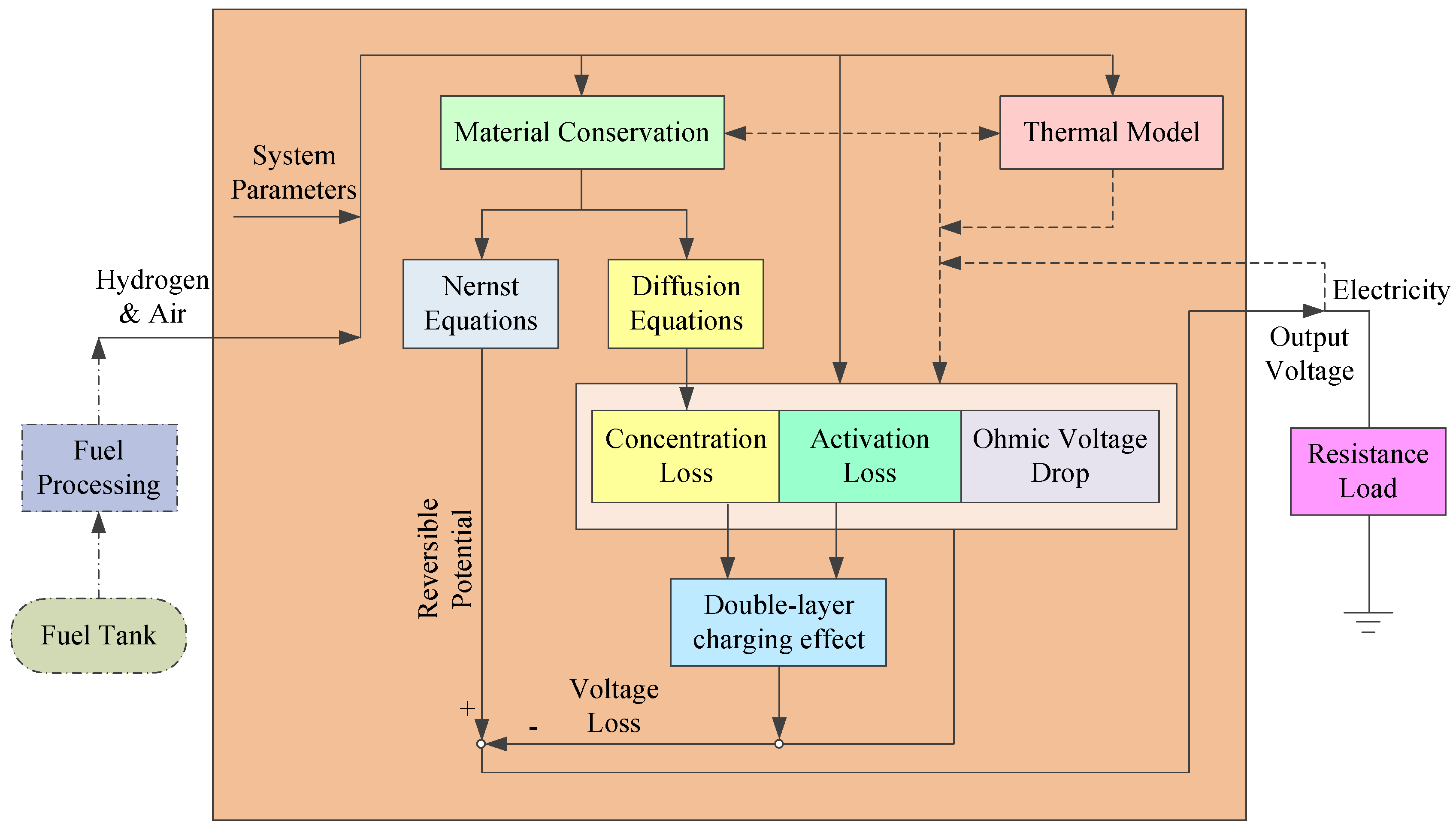
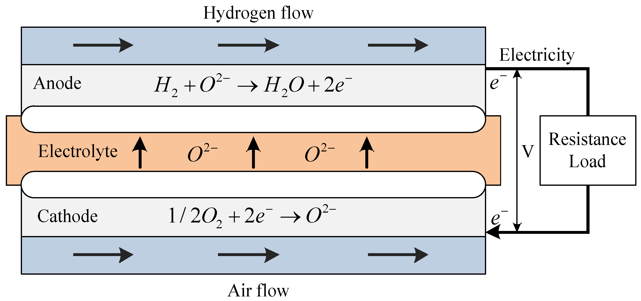
2. Dynamics and Nonlinearity Analysis of SOFC
3. MFPC Algorithm for SOFC
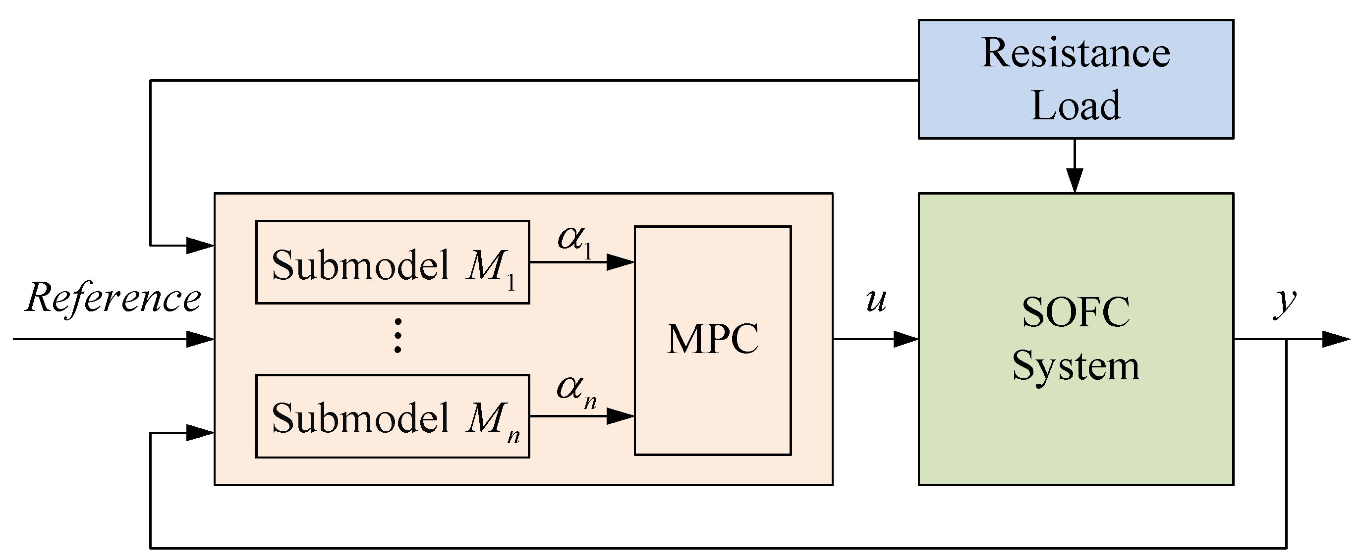
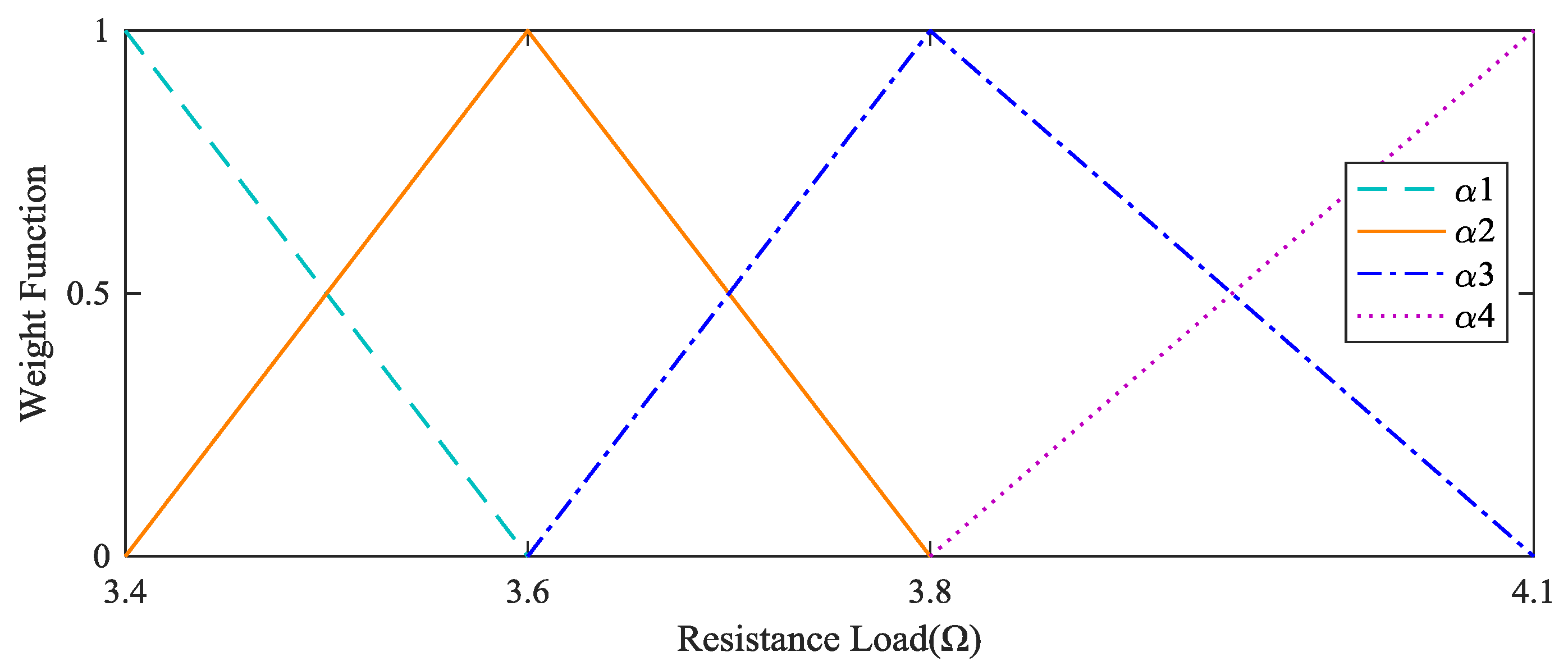
3.1. Multiple Model Strategy of SOFC
3.2. Predictive Model with Feedforward Compensation
3.3. Optimization Performance Index and Constrain
3.4. Feedback Correction
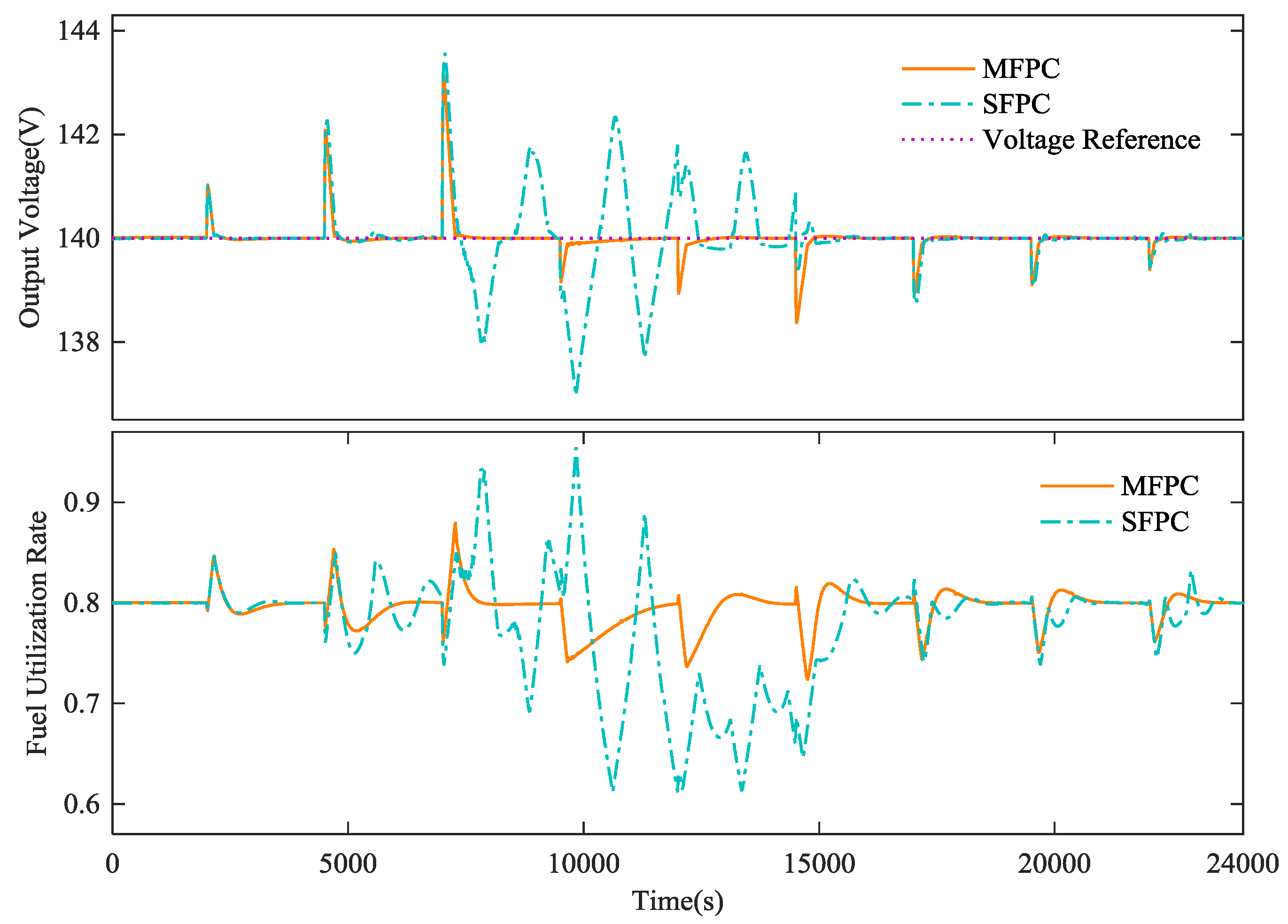
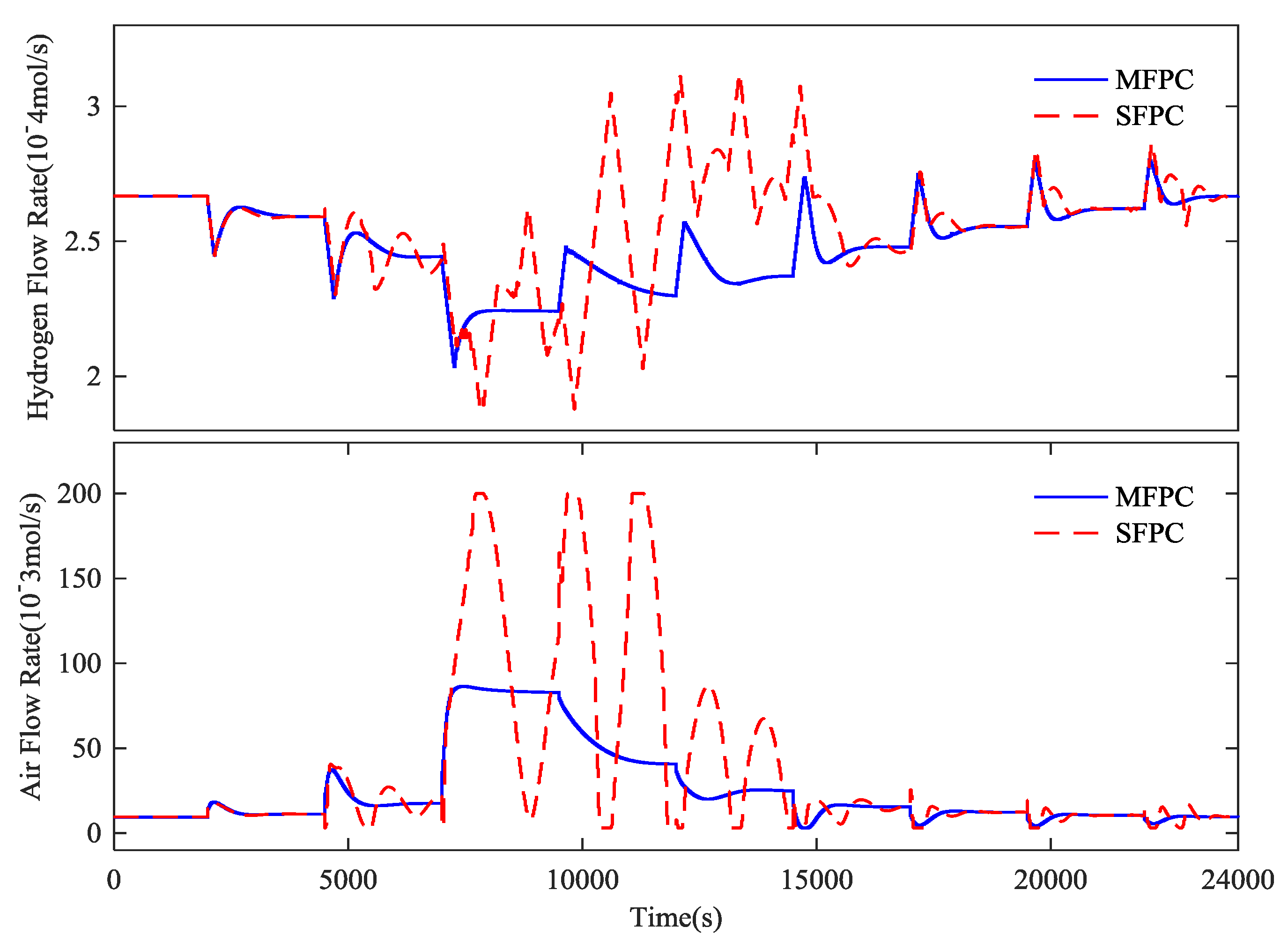
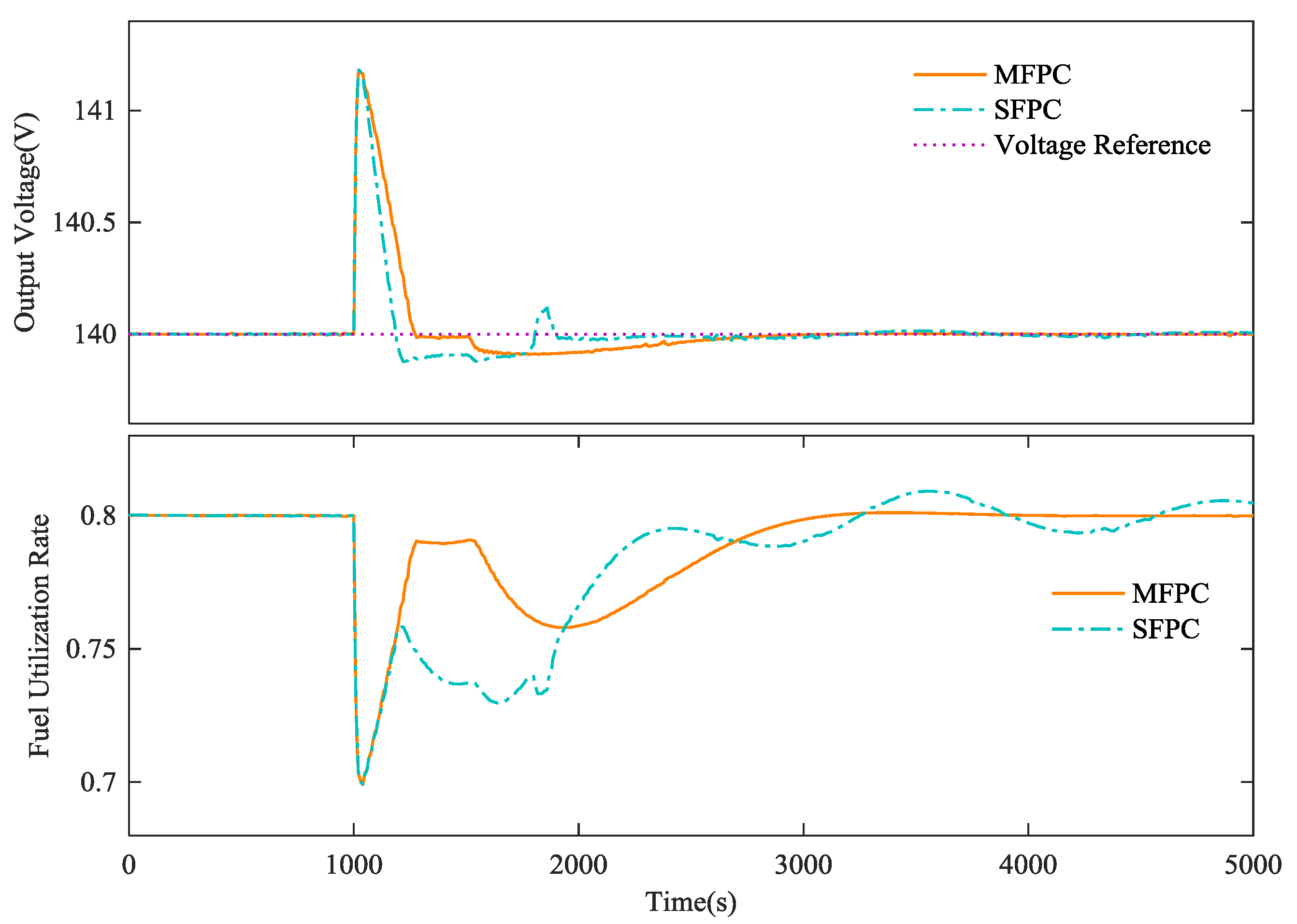
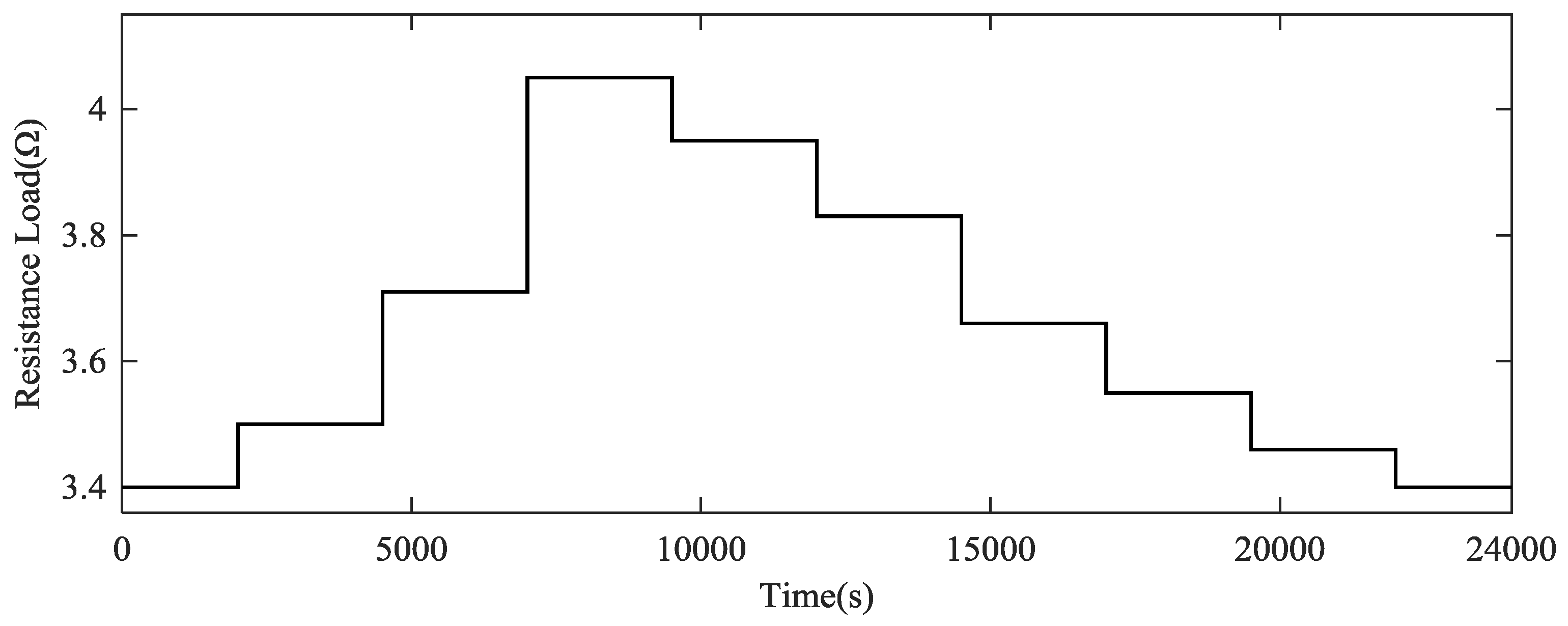
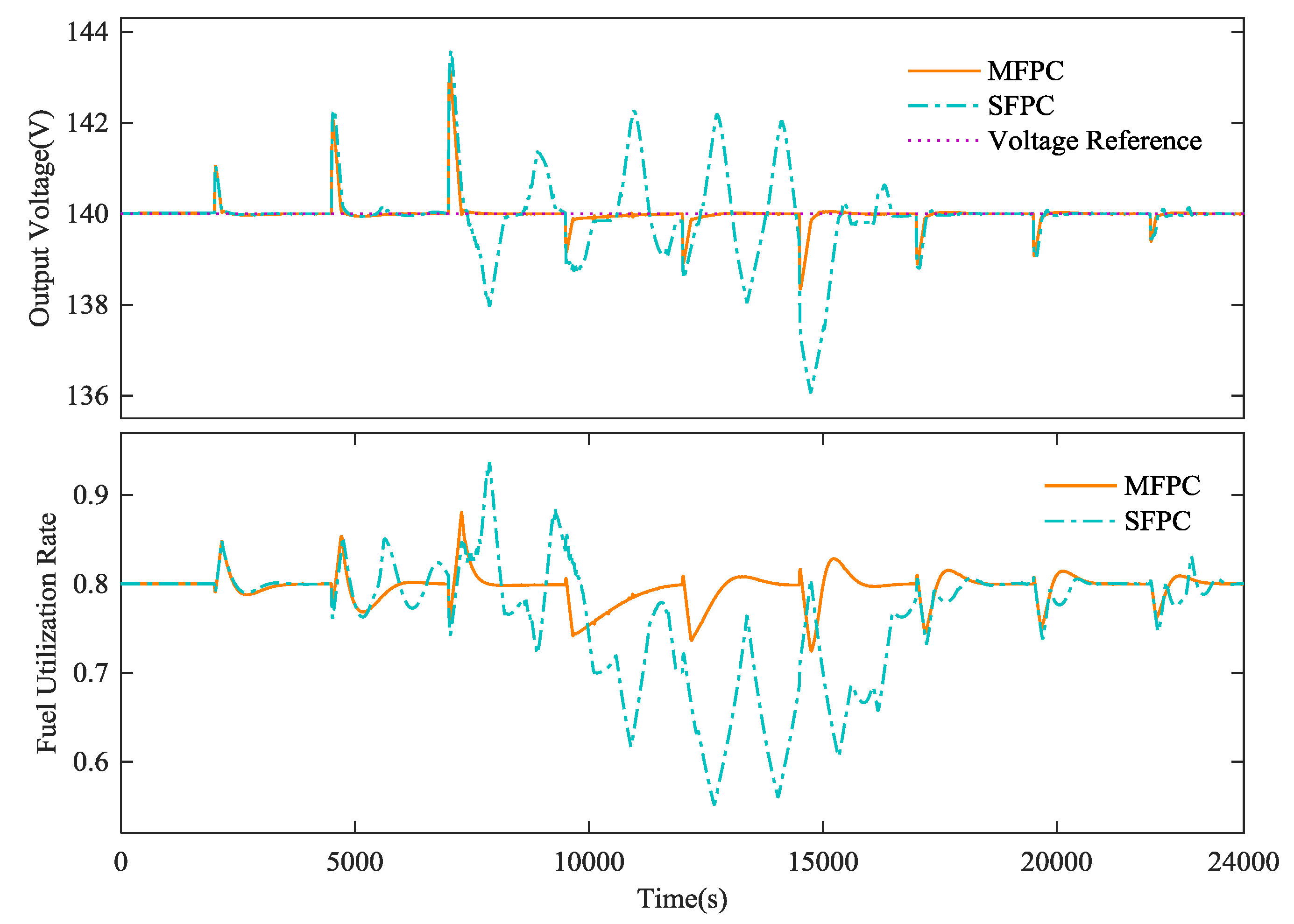
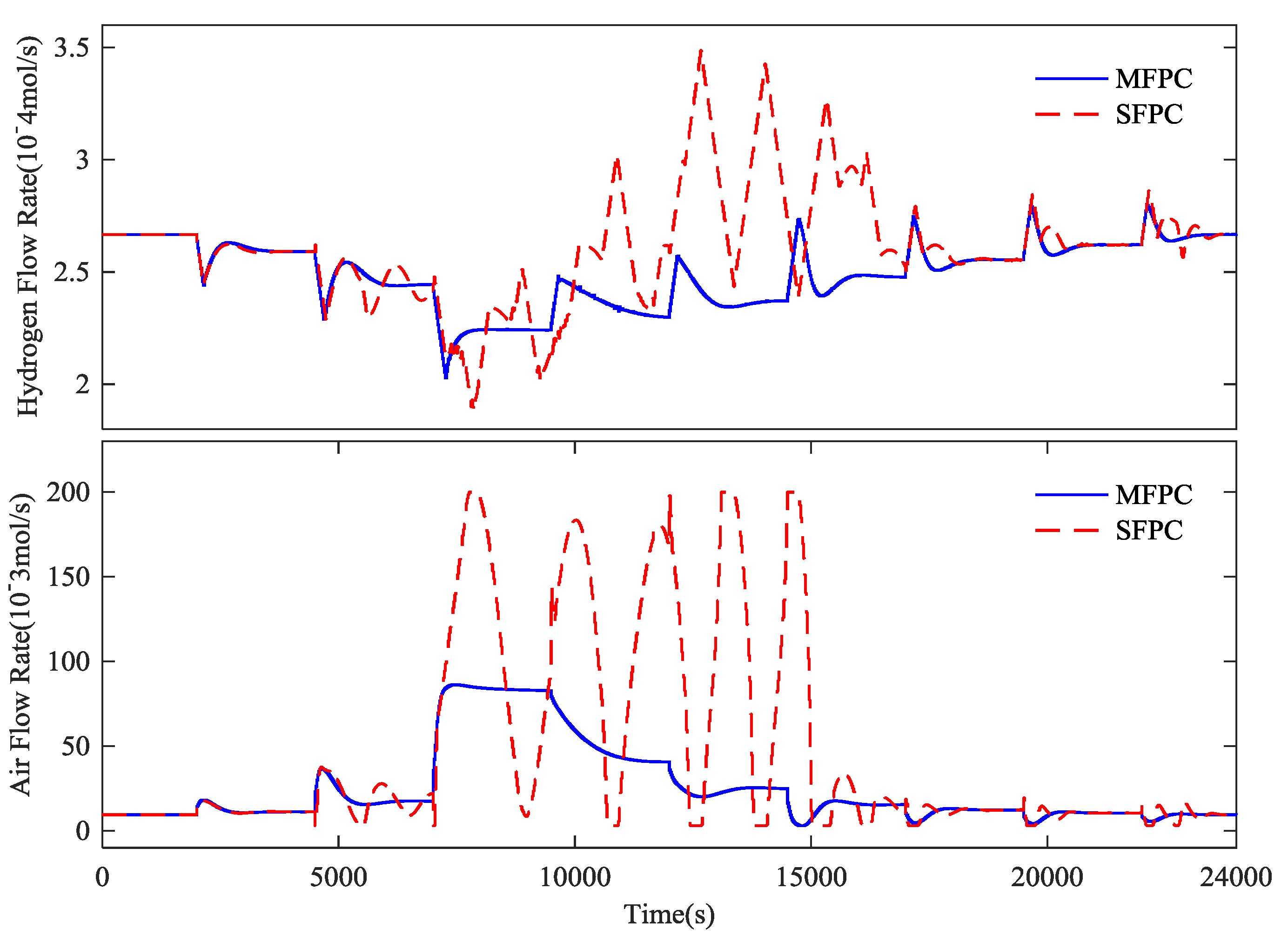
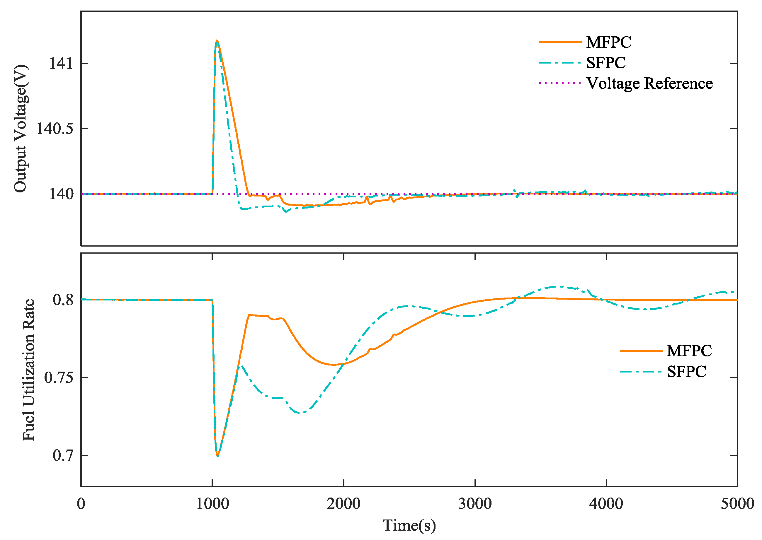
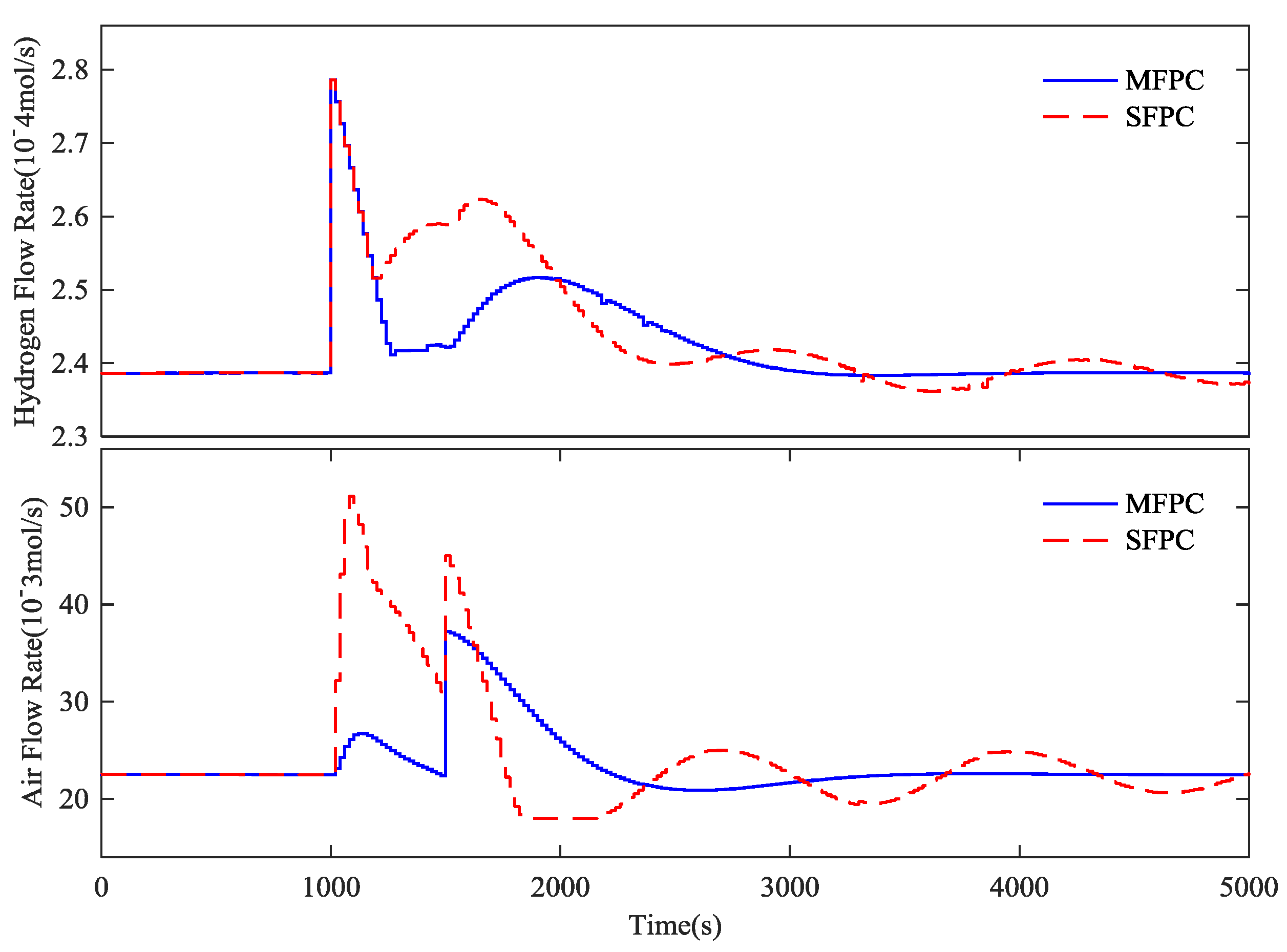
4. Simulation Results
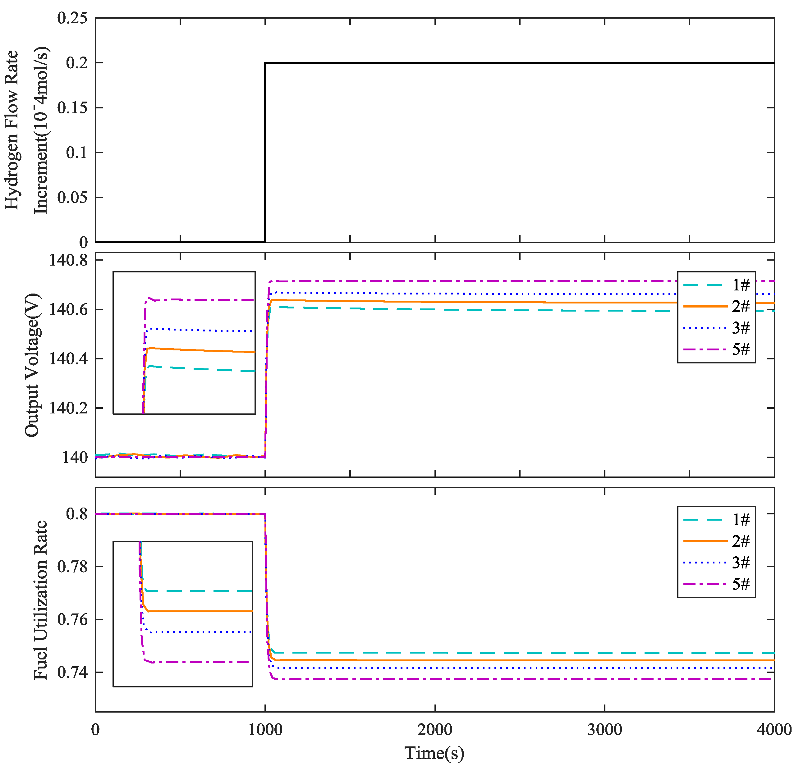
4.1. Case 1
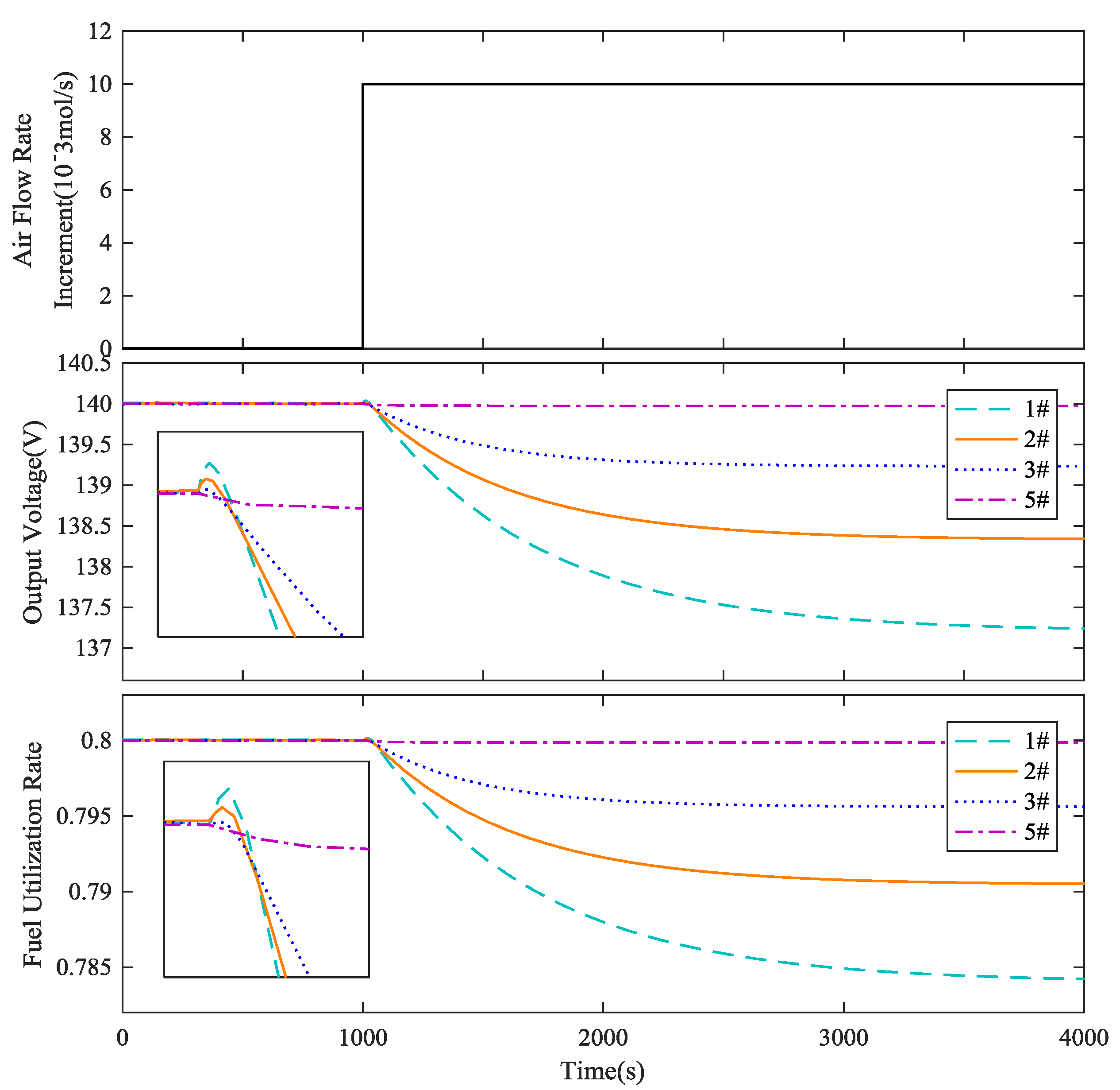
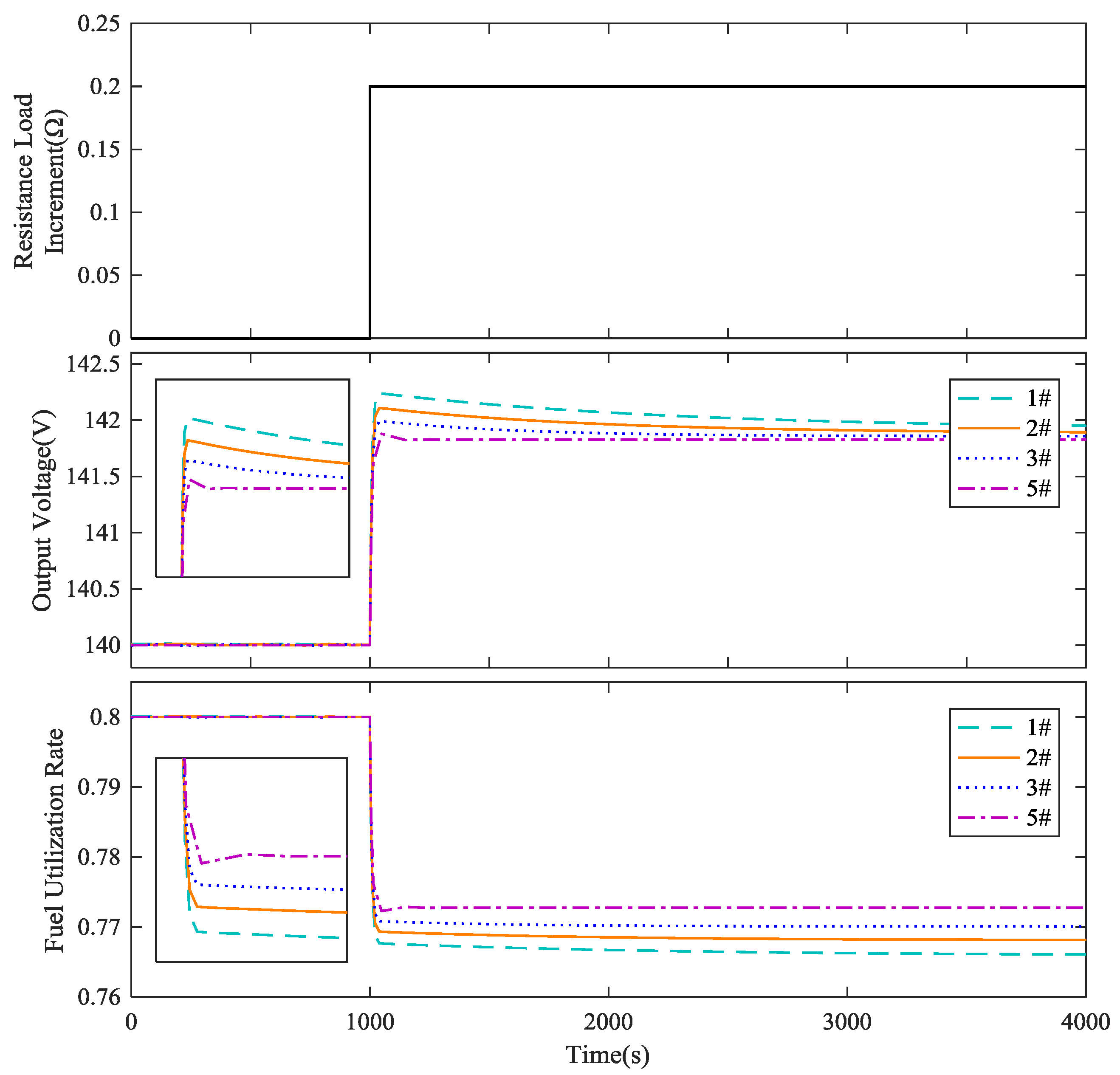
4.2. Case 2
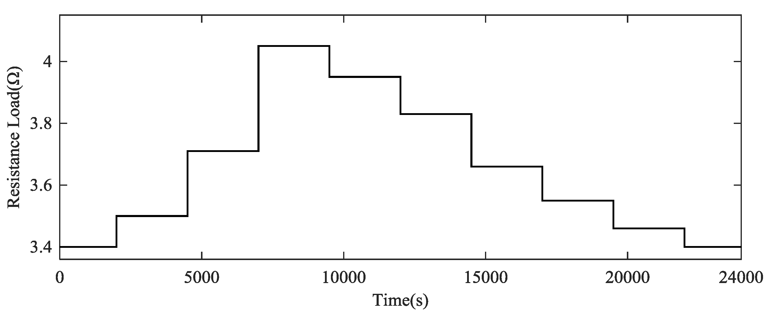
4.3. Case 3
5. Conclusions
Supplementary Materials
Acknowledgments
Author Contributions
Conflicts of Interest
References
- Dai, A.N.; Xu, L.F.; Shui, A.Z. Research Progress of Solid Oxide Fuel Cell. Bull. Chin. Ceram. Soc. 2015, 34, 234–238. [Google Scholar]
- Liu, X.L.; Ma, J. The development of Solid Oxide Fuel Cell Materials. Bull. Chin. Ceram. Soc. 2001, 20, 24–29. [Google Scholar]
- Lukas, M.D.; Lee, K.Y.; Ghezel-Ayagh, H. Development of a stack simulation model for control study on direct reforming molten carbonate fuel cell power plant. IEEE Trans. Energy Convers. 1999, 14, 1651–1657. [Google Scholar] [CrossRef]
- Lukas, M.D.; Lee, K.Y.; Ghezel-Ayagh, H. Modeling and cycling control of carbonate fuel cell power plants. Control Eng. Pract. 2002, 10, 197–206. [Google Scholar] [CrossRef]
- Cruz Rojas, A.; Lopez Lopez, G.; Gomez-Aguilar, J.F.; Alvarado, V.M.; Sandoval Torres, C.L. Control of the Air Supply Subsystem in a PEMFC with Balance of Plant Simulation. Sustainability 2017, 9, 73. [Google Scholar] [CrossRef]
- Huang, Z. Fuel Cell and Applications; Electronics Industry Press: Beijing, China, 2005. [Google Scholar]
- Buonomano, A.; Calise, F.; d’Accadia, M.D.; Palombo, A.; Vicidomini, M. Hybrid solid oxide fuel cells–gas turbine systems for combined heat and power: A review. Appl. Energy 2015, 156, 32–85. [Google Scholar] [CrossRef]
- Suther, T.; Fung, A.; Koksal, M.; Zabihian, F. Macro Level Modeling of a Tubular Solid Oxide Fuel Cell. Sustainability 2010, 2, 3549–3560. [Google Scholar] [CrossRef]
- Sun, L.; Wu, G.; Xue, Y.; Shen, J.; Li, D.; Lee, K.Y. Coordinated Control Strategies for SOFC Power Plant in a Microgrid. IEEE Trans. Energy Convers. 2017, PP, 1. [Google Scholar] [CrossRef]
- Singhal, S.C.; Kendall, K. High-Temperature Solid Oxide Fuel Cells: Fundamentals, Design and Applications; Elsevier: Amsterdam, The Netherland, 2002. [Google Scholar]
- Angrisani, G.; Roselli, C.; Sasso, M. Distributed microtrigeneration systems. Prog. Energy Combust. Sci. 2012, 38, 502–521. [Google Scholar] [CrossRef]
- Chicco, G.; Mancarella, P. Distributed multi-generation: A comprehensive view. Renew. Sustain. Energy Rev. 2009, 13, 535–551. [Google Scholar] [CrossRef]
- Zhao, F.; Zhang, C.H.; Sun, B.; Wei, D. Three-stage collaborative global optimization design mothod of combined cooling heating and power. Proc. CSEE 2015, 35, 3785–3793. [Google Scholar]
- Zhang, T.; Zhu, T.; Gao, N.; Wu, Z. Optimization design multi-criteria comprehensive evaluation method of combined cooling heating and power system. Proc. CSEE 2015, 35, 3706–3713. [Google Scholar]
- Ning-Sheng, C.A.; Chen, L.; Yi-Xiang, S.H. Research and development of solid oxide direct carbon fuel cell. Proc. CSEE 2011, 31, 112–120. [Google Scholar]
- Yu, Z.; Men, Q.; Zhang, C.; Han, J. Performance Analysis of the Near Zero CO2 Emissions Tri-generation System Based on Solid Oxide Fuel Cell Cycle. Proc. CSEE 2017, 37, 200–208. [Google Scholar]
- Kang, Y.W.; Cao, G.Y.; Tu, Y.Y.; Li, J. Output Voltage Feedforward—Feedback Control of Solid Oxide Fuel Cells. J. Eng. Therm. Energy Power 2008, 23, 97–101. [Google Scholar]
- Sun, L.; Li, D.; Wu, G.; Lee, K.Y.; Xue, Y. A Practical Compound Controller Design for Solid Oxide Fuel Cells. IFAC-PapersOnLine 2015, 48, 445–449. [Google Scholar] [CrossRef]
- Sun, L.; Hua, Q.; Shen, J.; Xue, Y.; Li, D.; Lee, K.Y. A Combined Voltage Control Strategy for Fuel Cell. Sustainability 2017, 9, 1517. [Google Scholar] [CrossRef]
- Li, Y.H.; Choi, S.S.; Rajakaruna, S. An analysis of the control and operation of a solid oxide fuel-cell power plant in an isolated system. IEEE Trans. Energy Convers. 2005, 20, 381–387. [Google Scholar] [CrossRef]
- Padulles, J.; Ault, G.W.; McDonald, J.R. An integrated SOFC plant dynamic model for power systems simulation. J. Power Sources 2000, 86, 495–500. [Google Scholar] [CrossRef]
- Wang, C.; Nehrir, M.H. A Physically Based Dynamic Model for Solid Oxide Fuel Cells. IEEE Trans. Energy Convers. 2007, 22, 887–897. [Google Scholar] [CrossRef]
- Gao, F.; Simoes, M.G.; Blunier, B.; Miraoui, A. Development of a Quasi 2-D Modeling of Tubular Solid-Oxide Fuel Cell for Real-Time Control. IEEE Trans. Energy Convers. 2014, 29, 9–19. [Google Scholar] [CrossRef]
- Bayati, M.; Abedi, M.; Gharehpetian, G.B. A new control system for grid-feeding power converters of solid oxide fuel cells. In Proceedings of the Iranian Conference on Electrical Engineering, Tehran, Iran, 2–4 May 2017; pp. 961–966. [Google Scholar]
- Hayati, M.R.; Khayatian, A.; Dehghani, M. Simultaneous Optimization of Net Power and Enhancement of PEM Fuel Cell Lifespan Using Extremum Seeking and Sliding Mode Control Techniques. IEEE Trans. Energy Convers. 2016, 31, 688–696. [Google Scholar] [CrossRef]
- Lan, T.; Strunz, K. Multi-Physics Transients Modeling of Solid Oxide Fuel Cells: Methodology of Circuit Equivalents and Use in EMTP-type Power System Simulation. IEEE Trans. Energy Convers. 2017, PP, 1. [Google Scholar]
- Yu, S.; Fernando, T.; Chau, T.K.; Iu, H.H. Voltage Control Strategies for Solid Oxide Fuel Cell Energy System Connected to Complex Power Grids Using Dynamic State Estimation and STATCOM. IEEE Trans. Power Syst. 2016, PP, 1. [Google Scholar] [CrossRef]
- Yu, S.; Fernando, T.; Iu, H.H. A Comparison Study for the Estimation of SOFC Internal Dynamic States in Complex Power Systems Using Filtering Algorithms. IEEE Trans. Ind. Inform. 2017, PP, 1. [Google Scholar] [CrossRef]
- Van Overschee, P.; De Moor, B.L. Subspace Identification for Linear Systems; Springer Science & Business Media: Berlin, Germany, 1996. [Google Scholar]


| Parameter | Representation | Unit |
|---|---|---|
| Gas constant | ||
| SOFC internal temperature | ||
| Faraday constant | ||
| Hydrogen partial pressure | ||
| Oxygen partial pressure | ||
| Water vapor partial pressure | ||
| Empirical constant | ||
| Anode channel volume | ||
| Time | ||
| Hydrogen flow rate of inlet | ||
| Hydrogen flow rate of outlet | ||
| Current | ||
| Water flow rate of inlet | ||
| Water flow rate of outlet | ||
| Cathode channel volume | ||
| Oxygen flow rate of inlet | ||
| Oxygen flow rate of outlet | ||
| Equivalent capacitance of the double-layer charging effect | ||
| Equivalent resistance of activation voltage drop | ||
| Equivalent resistance of concentration voltage drop | ||
| Constant term of activation voltage drop | ||
| Temperature coefficient | ||
| Equivalent resistance of ohmic voltage drop | ||
| Ohmic voltage drop of electrolyte | ||
| Ohmic voltage drop of interconnection |
| Operating Point | Resistance Load (Ω) | Hydrogen Flow Rate | Air Flow Rate | Output Voltage (V) | Fuel Utilization Rate |
|---|---|---|---|---|---|
| 1# | 3.4 | 2.667 | 9.5 | 140 | 0.8 |
| 2# | 3.6 | 2.520 | 13.5 | 140 | 0.8 |
| 3# | 3.8 | 2.386 | 22.3 | 140 | 0.8 |
| 4# | 4.0 | 2.267 | 55.0 | 140 | 0.8 |
| 5# | 4.1 | 2.211 | 165.0 | 140 | 0.8 |
| Parameter | Value |
|---|---|
| 20 s | |
| 30 | |
| 20 | |
| 2 | |
| diag [40, 550] | |
| diag [10, 1] | |
| [25, 200] | |
| [1, 3] | |
| [0.03, 50] | |
| [−0.03, −50] |
© 2018 by the authors. Licensee MDPI, Basel, Switzerland. This article is an open access article distributed under the terms and conditions of the Creative Commons Attribution (CC BY) license (http://creativecommons.org/licenses/by/4.0/).
Share and Cite
Wu, L.; Sun, L.; Shen, J.; Hua, Q. Multiple Model Predictive Hybrid Feedforward Control of Fuel Cell Power Generation System. Sustainability 2018, 10, 437. https://doi.org/10.3390/su10020437
Wu L, Sun L, Shen J, Hua Q. Multiple Model Predictive Hybrid Feedforward Control of Fuel Cell Power Generation System. Sustainability. 2018; 10(2):437. https://doi.org/10.3390/su10020437
Chicago/Turabian StyleWu, Long, Li Sun, Jiong Shen, and Qingsong Hua. 2018. "Multiple Model Predictive Hybrid Feedforward Control of Fuel Cell Power Generation System" Sustainability 10, no. 2: 437. https://doi.org/10.3390/su10020437
APA StyleWu, L., Sun, L., Shen, J., & Hua, Q. (2018). Multiple Model Predictive Hybrid Feedforward Control of Fuel Cell Power Generation System. Sustainability, 10(2), 437. https://doi.org/10.3390/su10020437