A Study on Heat-Transfer Characteristics by a Ground-Heating Method

Abstract

The ground-heating method using the electric heating pipe improves many problems of the conventional soft-ground improvement method and the ground-heating method using fossil fuel. However, in order to use this method practically, it is necessary to experimentally verify the temperature change due to the discharge of water vapor, and also to compare the theoretical solution and numerical analysis for estimation of the temperature distribution. From the experimental result, the loss of heat energy due to the discharge of water vapor is very large. Because the linear heat-source model and numerical analysis cannot consider the heat-energy loss by water vapor, the temperature change is estimated to be large. Therefore, it is necessary to design the installation depth of the electric heating pipe to suppress the discharge of water vapor.

1. Introduction

In order to use industrial and residential land, we are developing soft grounds such as tidal flats. General soft-ground improvement methods are the preloading and the vertical drainage. In both methods, marine clays such as tidal flats have a very small permeability, so that excess pore water pressure is generated by the preloading of embankment, and it is drained by the vertical drainage of sand. However, because this method requires a large amount of sand, deforestation and land degradation are serious [1]. Furthermore, because the permeability of the clay is very small, the consolidation of clay takes about five to 10 years to complete [2].

To solve this problem, Beles and Stănculescu [3], and Litvinov [4], developed a ground-heating method using fossil fuels. It is a method of burning after pressurizing fossil fuel mixed with air into the bore holes on the soft ground. Because fossil fuel and air burn at temperatures of 600–800 °C into the bore holes, the state of the clay rapidly changes from a saturated liquid to a dried solid. Most of the soil is non-plastic at 400–600 °C [5,6,7,8,9]. As a result, the strength of the clay sintered by the ground heating is rapidly increased, and the ground can be improved and utilized as a construction site [4,9,10,11].

However, the ground-heating method using the fossil fuels has not been widely applied due to many problems. The entire system of the ground-heating method proposed by Litvinov [4] is very complicated due to the compressor, pipeline for cold air, a container for liquid fuel, pump for supplying fuel under pressure into the bore hole, fuel pipeline, filters, nozzle, and the cover with the combustion chamber. Furthermore, the operation of this system requires highly skilled engineers. Finally, the cost of fossil fuels is high, and the economy is low [1].

In recent years, Park, Im, Shin and Han [1] proposed a ground-heating method in which fossil fuel use was improved with the electric heating pipe. The electric heating pipe converts the electric energy into thermal energy by the electric-resistance method, and is applied to the improvement of the strength of the soft ground. They heated the depth of soft ground up to 1.0 m, and confirmed the trafficability of the construction equipment. Park et al. [12] conducted the experiment of a comparison of the consolidation settlement of the pre-loading with vertical drain, and the ground-heating method using the electric heating pipe. As the result showed, the dissipation of pore water and the consolidation effect were remarkably better by the ground-heating method in the laboratory scale. Park, Lee, Jang and Han [2] studied the temperature change on the soft ground by the ground-heating pipe. The soft ground of the silty sand was heated by an electric heating pipe and the temperature change of the ground was measured. The experimental results were compared with a theoretical solution and a numerical analysis. The temperature change from the heat source, the electric heating pipe, was shown to be a logarithmic decreasing function. Additionally, there was a larger temperature change in the vertical direction than in the horizontal direction from the heat source.

The effect of the ground-heating method using the electric heating pipe has been verified, but it is necessary to solve many engineering problems in order to put it to practical use. Park, Im, Lee and Han [12] reported that a large amount of water vapor is discharged to the ground surface due to the ground heating. However, since the discharge of water vapor is a heat loss, it is necessary to experimentally verify how the temperature changes according to the presence or absence of discharge of water vapor in the ground-heating process. For the design of this method, the temperature change due to the ground heating should be calculated by theoretical solution and numerical analysis. However, these techniques do not consider the heat loss due to the discharge of water vapor. Therefore, it is necessary to compare these techniques with experimental results performed in the presence or absence of discharge of water vapor.

The ground-temperature distribution generally uses Kelvin’s linear source model, which is used for the design of the ground heat exchanger. For the ground heat exchanger, much research has been done on evaluation of thermal conductivity for grout/soil formation using thermal response [13]. The ground heat exchanger has a small difference and variation in temperature between the heat source and the ground. Because the ground-heating method has a large temperature difference between the heat source and the ground, and heat loss due to water vapor is generated, it is necessary to verify the linear heat-source model to estimate the temperature distribution of the ground-heating method. Finally, the numerical analysis to estimate the temperature distribution is mainly used for the study of geothermal phenomena, and freezing and thawing on the ground [14]. Most of these studies have been conducted on heat-transfer processes by climatic conditions or pipelines. There are not many cases in which ground temperature changes due to high-temperature heat sources (such as the ground-heating method) are estimated.

In this study, two case experiments were conducted to investigate the temperature changes of the ground, depending on whether water vapor was discharged or not. Then, the linear heat-source model as the theoretical solution and numerical analysis was performed and compared with experimental results. In the first case, an electric heating pipe was exposed to the surface of the soil so that water vapor could be discharged. The second case was installed at a depth of 30 cm from the surface to prevent water vapor from being discharged. This experiment was based experiments on the thermal conductivity of soil [15,16] and with experiments performed by Park, Im, Lee and Han [12]. Compared with the previous studies, the sensor for measuring the ground temperature was the same, and the heat source was an electric heating tube manufactured for this study. Unlike previous studies, the electric heating pipe was heated to 450 °C using a DC power supply. Additionally, kaolinite, a standard clay, was used. Numerical analysis was performed with Temp/W of Geostudio under the same conditions as the experiment.

2. Theoretical Solution and Numerical Analysis

2.1. Theoretical Solution Using Linear Heat-Source Model

The change of ground temperature by the ground heating is estimated by Kelvin’s linear heat-source model, which is applied to a ground heat exchanger in Figure 1 [17]. If the linear heat source is infinitely long, the heat flux is constant and the initial temperature is ${\mathrm{T}}_0$, the temperature distribution in the ground is as shown in Equation (1),

$$\mathrm{T}\left(\mathrm{r},\mathrm{t}\right)-{\mathrm{T}}_0=\frac{\mathrm{Q}/\mathrm{L}}{4\mathsf{\pi }\mathrm{k}}{{\displaystyle \int }}_{\mathrm{x}}^{\infty }\frac{{\mathrm{e}}^{-\mathrm{u}}}{\mathrm{u}}\mathrm{du},$$

(1)

where $\mathrm{T}\left(\mathrm{r},\mathrm{t}\right)$ is the temperature (°C) in the distance of r ($\mathrm{m}$) from the linear heat source and at the time of t (s); $\mathrm{k}$ is the thermal conductivity W/m °C; $\mathrm{Q}$ is the heat-extraction rate to be transferred to the soil $\left(\mathrm{W}\right)$; and $\mathrm{L}$ is the length of the ground heat exchanger ($\mathrm{m}$).

Therefore, $\mathrm{Q}/\mathrm{L}$ is the heat-transfer rate divided by the heat-extraction rate ($\mathrm{W}/\mathrm{m}$) per the unit length of the ground heat exchanger. The soil’s thermal diffusivity is shown in Equation (2),

$$\mathrm{k}=\frac{{\mathrm{r}}^2}{4\mathrm{at}},$$

(2)

where a (m²/s) is the soil’s thermal diffusivity defined as $\mathrm{k}/\mathsf{\rho }\mathrm{c}$ ($\mathsf{\rho }$ is the density of soil (kg/m³), and c (kJ/kg °C) is the specific heat of soil), and pc (kJ/m³ °C) is the volumetric heat capacity of soil. Because the heat source is assumed to be infinitely long, all the heat flow is in the horizontal direction perpendicular to the heat source.

The integral term on the right side of Equation (1) is the exponential integral, which is expressed as ${\mathrm{E}}_{\mathrm{i}}\left(\mathrm{x}\right)$ and which appears in infinitive series as seen in Equation (3),

$${\mathrm{E}}_{\mathrm{i}}={{\displaystyle \int }}_{\mathrm{k}}^{\infty }\frac{{\mathrm{e}}^{-\mathrm{u}}}{\mathrm{u}}\mathrm{du}={{\displaystyle \int }}_{\frac{{\mathrm{r}}^2}{4\mathrm{at}}}^{\infty }\frac{{\mathrm{e}}^{-\mathrm{u}}}{\mathrm{u}}\mathrm{du}=\mathrm{r}-\ln \mathrm{k}+\left(\frac{\mathrm{k}}{1·1!}-\frac{{\mathrm{k}}^2}{2·2!}+\frac{{\mathrm{k}}^3}{3·3!}\cdots \right),$$

(3)

where $\mathrm{r}$ is Euler’s constant, which is recorded at $0.5772$. In Equation (3), if the $\mathrm{k}$ value is small, ${\mathrm{E}}_{\mathrm{i}}\left(\mathrm{x}\right)$ can be expressed only with the first four terms, as seen in Equation (4).

$${\mathrm{E}}_{\mathrm{i}}\left(\mathrm{x}\right)=-\mathrm{r}-\ln \mathrm{k}+\mathrm{k}-\frac{1}{4}{\mathrm{k}}^2\cdots$$

(4)

Therefore, Equation (1) can be converted into Equation (5).

$$\mathrm{T}\left(\mathrm{r},\mathrm{t}\right)-{\mathrm{T}}_0=\frac{\mathrm{Q}/\mathrm{L}}{4\mathsf{\pi }\mathrm{k}}\left\{-\mathrm{r}-\ln \frac{{\mathrm{r}}^2}{4\mathrm{at}}+\frac{{\mathrm{r}}^2}{4\mathrm{at}}-\frac{1}{4}{\left(\frac{{\mathrm{r}}^2}{4\mathrm{at}}\right)}^2\right\}=\frac{\mathrm{Q}/\mathrm{L}}{4\mathsf{\pi }\mathrm{k}}\left\{\ln \frac{4\mathrm{at}}{{\mathrm{r}}^2}-\mathrm{r}+\frac{{\mathrm{r}}^2}{4\mathrm{at}}\left(1-\frac{{\mathrm{r}}^2}{16\mathrm{at}}\right)\right\}$$

(5)

According to Carslaw and Jaeger [18], Equation (5) can be approximated as Equation (6). Equation (6) is the approximation formula of Equation (5), which is known to have the margin of error of up to 2% in the case of $\mathrm{at}/{\mathrm{r}}^2>5$.

$$\mathrm{T}\left(\mathrm{r},\mathrm{t}\right)-{\mathrm{T}}_0=\frac{\mathrm{Q}/\mathrm{L}}{4\mathsf{\pi }\mathrm{k}}\left(\ln \frac{4\mathrm{at}}{{\mathrm{r}}^2}-\mathrm{r}\right)$$

(6)

For analysis of temperature changes caused by ground heating, the initial underground temperature in Equation (6) is transposed to the right-hand side, which is then substituted with Euler’s constant as seen in Equation (7). Equation (7) is the equation of the linear heat-source model by ground heating,

$$\mathrm{T}\left(\mathrm{r},\mathrm{t}\right)={\mathrm{T}}_0+\frac{\mathrm{Q}/\mathrm{L}}{4\mathsf{\pi }\mathrm{k}}\left(\ln \frac{4\mathrm{at}}{{\mathrm{r}}_{\mathrm{b}}{}^2}-0.5772\right),$$

(7)

where the variables of the ground include the initial underground temperature (°C) of ${\mathrm{T}}_0$, the thermal conductivity $\left(\mathrm{W}/\mathrm{m}·\mathrm{K}\right)$ of $\mathrm{k}$, and the thermal diffusivity (m²/s) of $\mathsf{\alpha }$. The variables of the electric heating pipe include the radius ($\mathrm{m}$) of ${\mathrm{r}}_{\mathrm{b}}$, the length ($\mathrm{m}$) of $\mathrm{L}$, and the start-up parameter ($\mathrm{W}$) of $\mathrm{Q}$. $\mathrm{t}$ is the operation time ($\mathrm{s}$), and $\mathrm{r}$ is the horizontal distance from the heat source ($\mathrm{m}$).

2.2. Numerical Analysis

The heat-transfer model applied to the numerical analysis is as follows. Applying the Galerkin method of weighed residuals to the governing differential equation, the finite element for the two-dimensional thermal equation can be derived as [19]:

$$\mathsf{\tau }{{\displaystyle \int }}_{\mathrm{A}}^{}({\left[\mathrm{B}\right]}^{\mathrm{T}}\left[\mathrm{C}\right]\left[\mathrm{B}\right])\mathrm{dA}\left\{\mathrm{T}\right\}+\mathsf{\tau }{{\displaystyle \int }}_{\mathrm{A}}^{}({\mathsf{\lambda }\langle \mathrm{N}\rangle }^{\mathrm{T}}\langle \mathrm{N}\rangle )\mathrm{dA}\left\{\mathrm{T}\right\},\mathrm{t}=\mathrm{q}\mathsf{\tau }{{\displaystyle \int }}_{\mathrm{L}}^{}({\langle \mathrm{N}\rangle }^{\mathrm{T}})\mathrm{dL},$$

(8)

where $\left[\mathrm{B}\right]$ is the gradient matrix, $\left[\mathrm{C}\right]$ is the element thermal conductivity matrix, $\left\{\mathrm{T}\right\}$ is the vector of nodal temperatures, $\langle \mathrm{N}\rangle$ is the vector of interpolating function, $\mathrm{q}$ is the unit flux across the edge of an element, $\mathsf{\tau }$ is the thickness of an element, $\mathrm{t}$ is time, $\mathsf{\lambda }$ is the capacity for heat storage, $\mathrm{A}$ is a designation for summation over the area of an element, and $\mathrm{L}$ is a designation for summation over the edge of an element.

The finite-element solution for a transient analysis is a function of time as indicated by the $\left\{\mathrm{T}\right\},\mathrm{t}$ term in the finite-element equation [20]. The time integration can be performed by a finite-difference approximation scheme. Writing the finite-element equation in terms of finite differences leads to the following equation [19]:

$$\left(\mathsf{\omega }\Delta \mathrm{t}\left[\mathrm{K}\right]+\left[\mathrm{M}\right]\right)\left\{{\mathrm{T}}_1\right\}=\Delta \mathrm{t}\left(\left(1+\mathsf{\omega }\right)\left\{{\mathrm{Q}}_0\right\}+\mathsf{\omega }\left\{{\mathrm{Q}}_1\right\}\right)+\left(\left[\mathrm{M}\right]-\left(1-\mathsf{\omega }\right)\Delta \mathrm{t}\left[\mathrm{K}\right]\right)\left\{{\mathrm{T}}_0\right\},$$

(9)

where t is the time increment, $\mathsf{\omega }$ is a ratio between 0 and 1, ${\mathrm{T}}_1$ is the temperature at end of time increment, ${\mathrm{T}}_0$ is the temperature at start of time increment, ${\mathrm{Q}}_1$ is the nodal flux at end of time increment, and ${\mathrm{Q}}_0$ is the nodal flux at start of time increment.

The finite-element solution for a transient analysis has temperature changes being a function of time as indicated by the $T_1$ term in the finite-element equation (Equation (10)). In order to solve for the temperature at some point in the future, time integration can be performed by a finite-difference approximation scheme. Writing the finite-element equation in terms of a “backward difference” finite-difference form leads to the following equation [19]:

$$\left\{{\mathrm{T}}_1\right\}=\frac{\Delta \mathrm{t}\left\{{\mathrm{Q}}_1\right\}+\left[\mathrm{M}\right]\left\{{\mathrm{T}}_0\right\}}{\Delta \mathrm{t}\left[\mathrm{K}\right]+\left[\mathrm{M}\right]},$$

(10)

where $\Delta \mathrm{t}$ is the time increment, ${\mathrm{T}}_1$ is the temperature at end of time increment, ${\mathrm{T}}_0$ is the temperature at start of time increment, $\left\{{\mathrm{Q}}_1\right\}$ is the nodal flux at end of increment, $\left[\mathrm{K}\right]$ is the element thermal conductivity matrix, and $\left[\mathrm{M}\right]$ is the element heat-storage matrix.

3. Characteristics of Heat Transfer Due to Vapor Discharge

3.1. Ground Heating and Measurement System (Case 1)

Electric heating pipes that are generally used in the industrial field are made up of heating wires, protective tubes and the heat-transfer medium of magnesia (MgO). The Korea standard electric wires can be classified into nickel–chromium type 1, nickel–chromium type 2, iron–chromium type 1, iron–chromium type 2, and so on [21], and this study used nickel–chromium type 1. Protective tubes are made of iron, copper and stainless steel, and this study used a stainless steel tube (SUS 304). Magnesia, the heat-transfer medium, has an excellent heat conductivity at a high temperature compared to other ceramic materials, as it has good electrical insulation properties. Apart from transferring heat, magnesia plays the role of preventing a short circuit by fixing electric heating wires inside the protective tube.

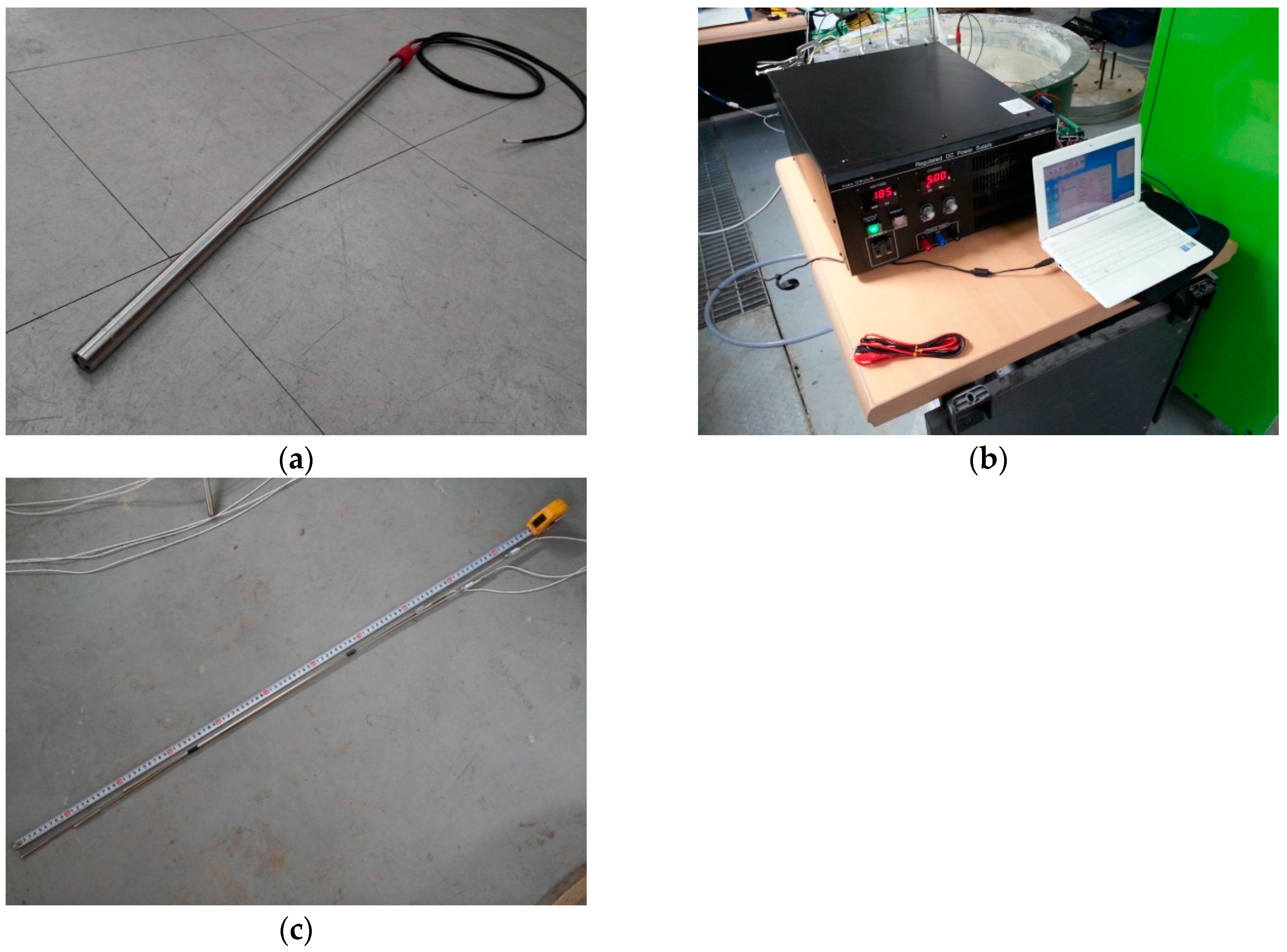
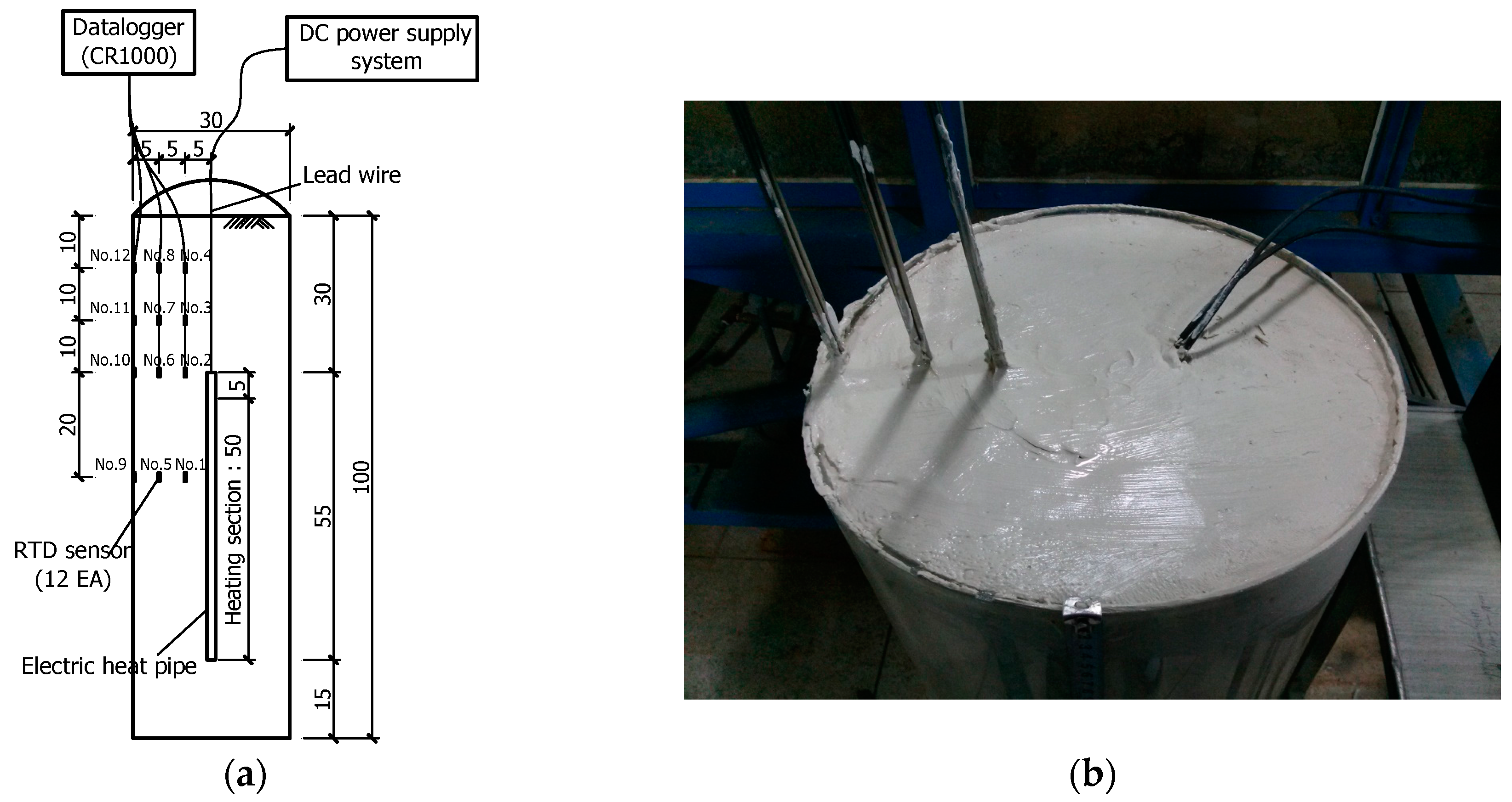
The electrical heating pipe used in this study, as shown in Figure 2a, has a total length of 60 cm, which has a heating section of 55 cm and a nonheating section of 5 cm, with a diameter of 22.7 mm. The electric heating pipe was supplied with a constant direct current by using a DC power supplier (Figure 2b). In the experiment, an electric heating pipe consumes electric power of about $925\mathrm{W}$ per hour, and the surface temperature is 500 °C. A resistance temperature detector (PT100) was used as a thermometer, and the temperature measurement range was 0 to 700 °C measured at intervals of 10 min.

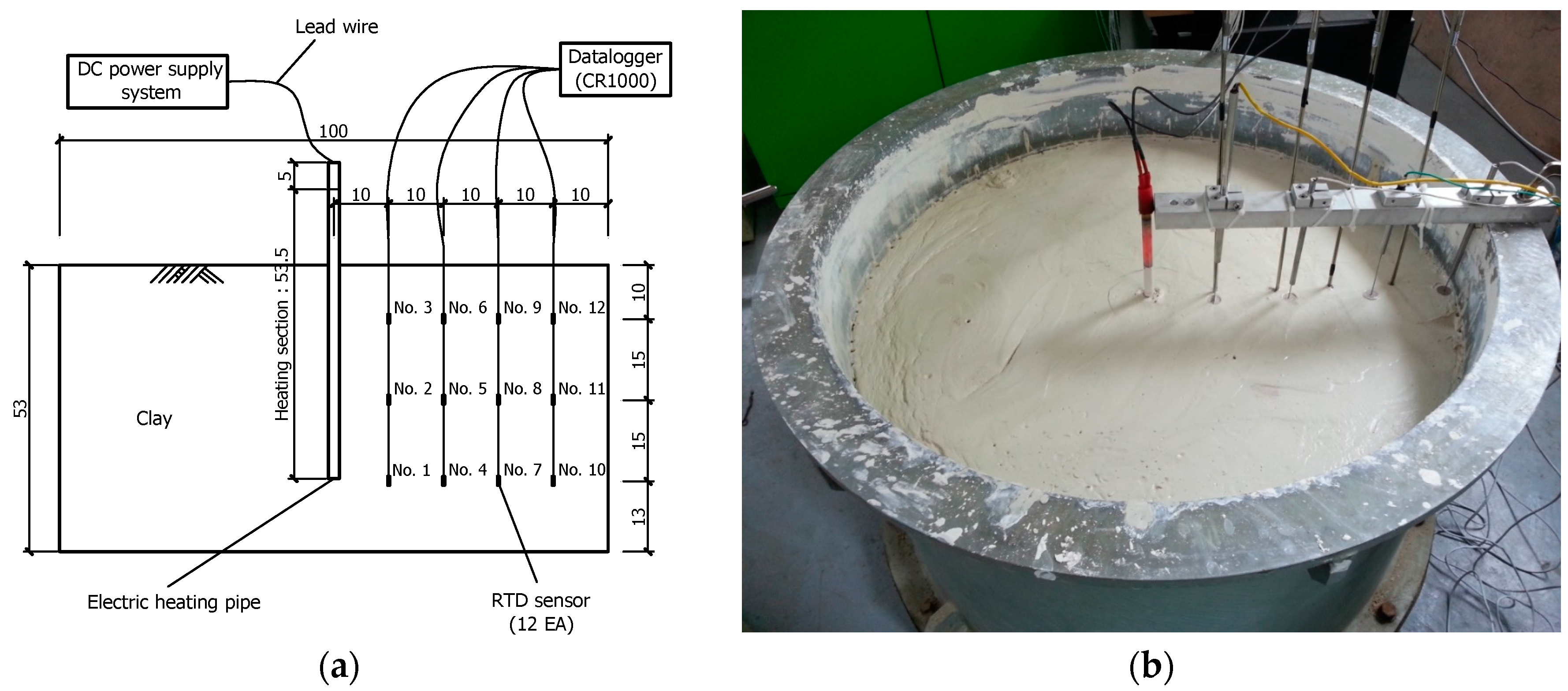
The soil box was made in a round shape with a diameter of 100 cm and a height of 67 cm using steel. In order to drain the pore water by self-weight consolidation, a membrane was installed at the bottom of the soil box. The soil used in the experiment was kaolinite, a standard clay, and stirred at a water content of two times the liquid limit with a vacuum stirrer. The agitated standard clay was filled in the soil box and self-weight consolidation occurred for about six months, while the height of the standard clay was about 53 cm.

An electric heating pipe with a total length of 58.5 cm was interpenetrated and installed 40 cm deep into the middle of the soil box filled with the standard clay. The thermometers were positioned in four rows at a 10 cm interval in the horizontal direction and in three columns at 10 cm, 25 cm and 40 cm depths from the surface in the vertical direction (Figure 3).

Ground heating was carried out for two days and the temperatures were measured for seven days in order to find out temperature increases by ground heating as well as temperature decreases after the end of heating.

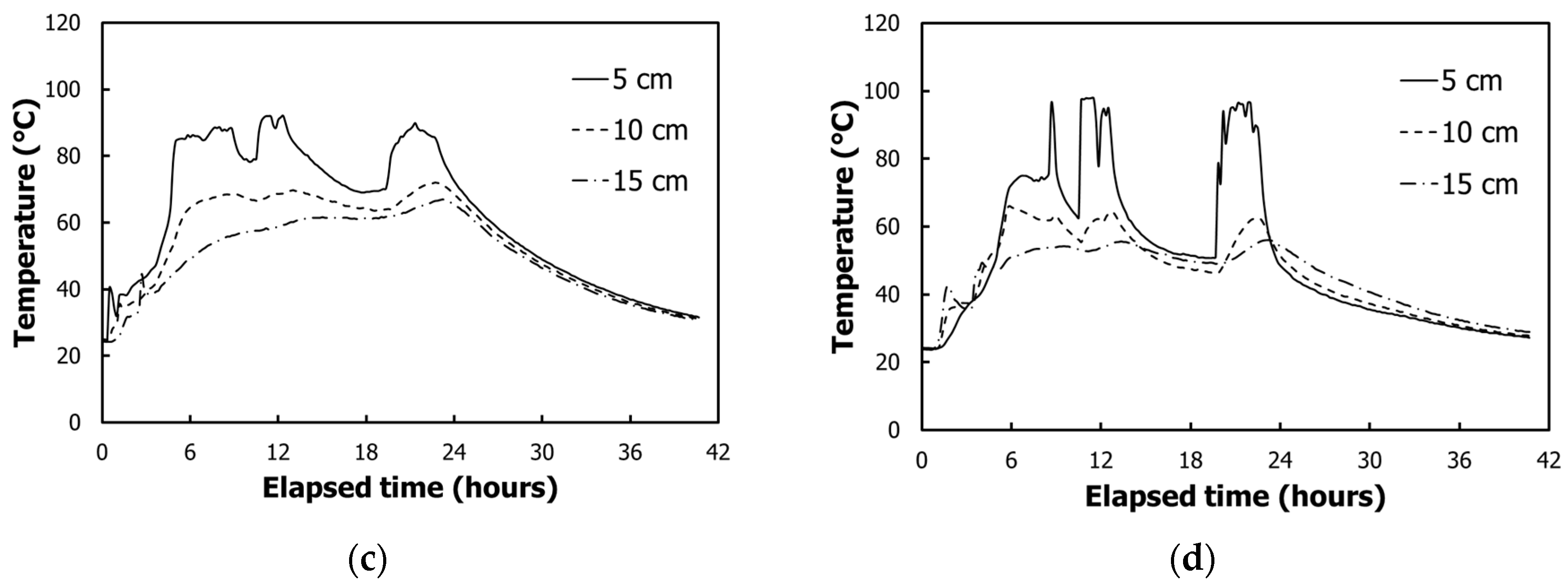
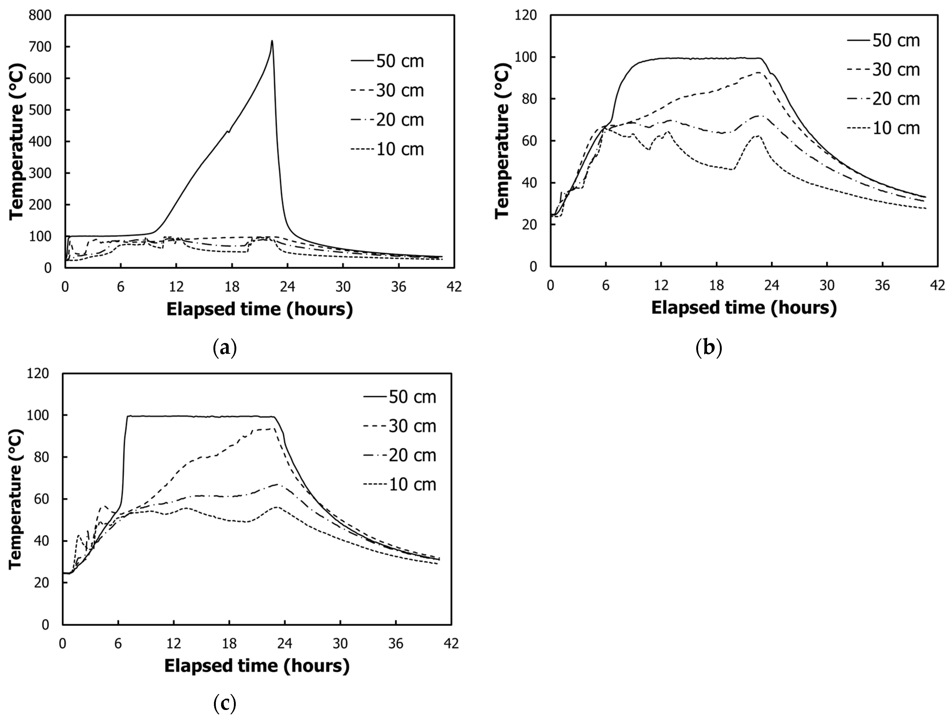
3.2. Temperature Measurement Results (Case 1)

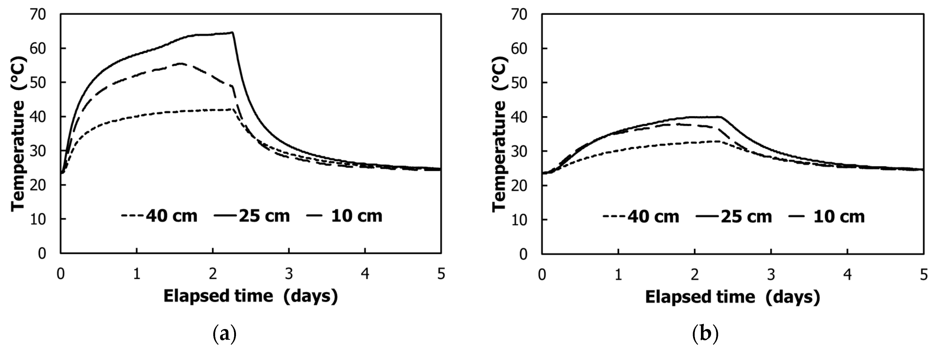
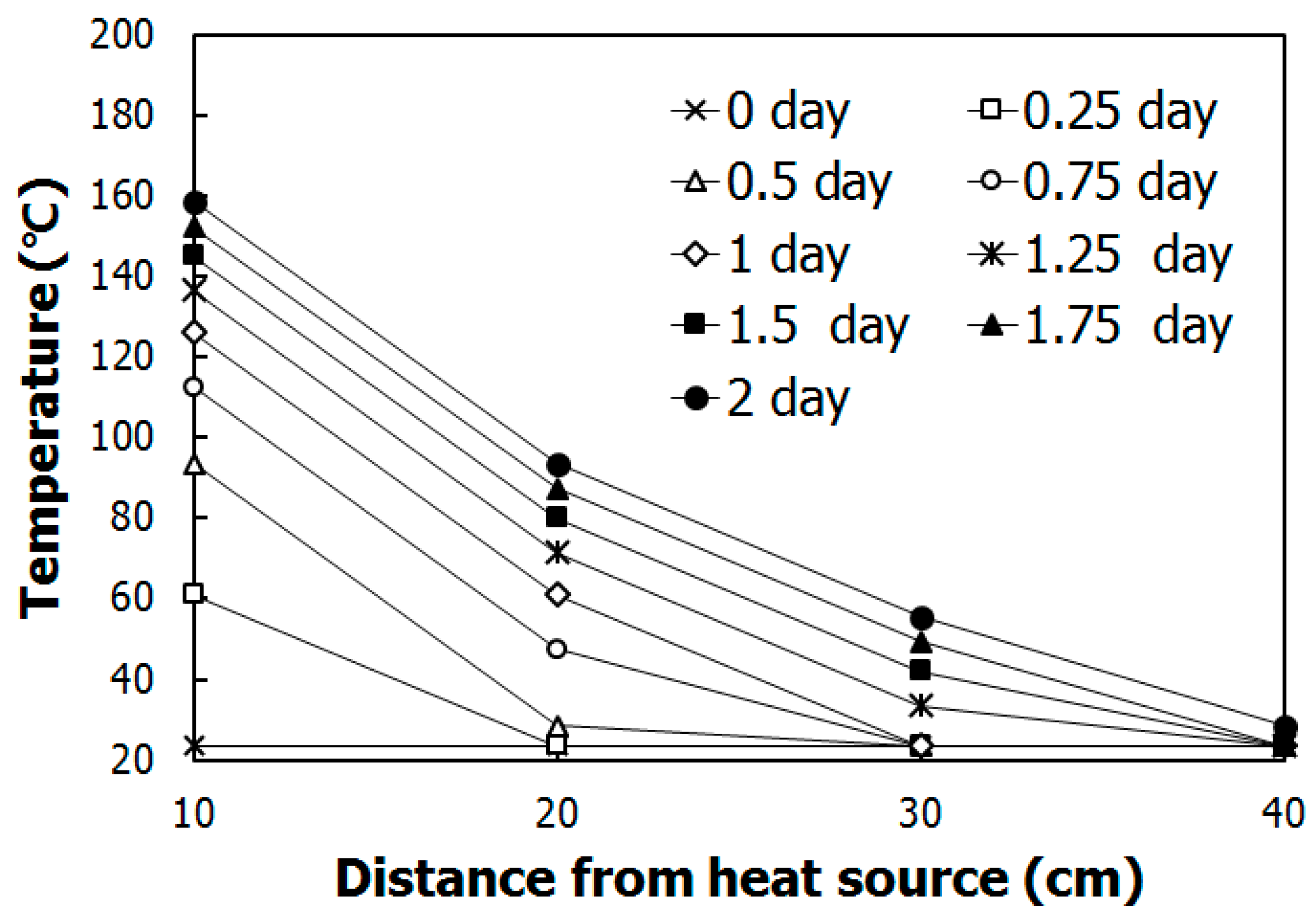
Figure 4 shows the temperature changes according to underground depths. Figure 4a shows temperature changes in sensors installed 10 cm away in a horizontal direction from the heat source at the respective underground depths. Temperature changes were almost the same, but the lowest temperature change was recorded at spots 40 cm away from the heat source, while the greatest temperature change was observed at the underground depth of 25 cm. Figure 4b–d shows the temperature changes in the sensors installed 20 cm, 30 cm and 40 cm from the heat source in a horizontal direction at each underground depth. The largest temperature variation was recorded at the ground depth of 25 cm, as seen in Figure 4a.

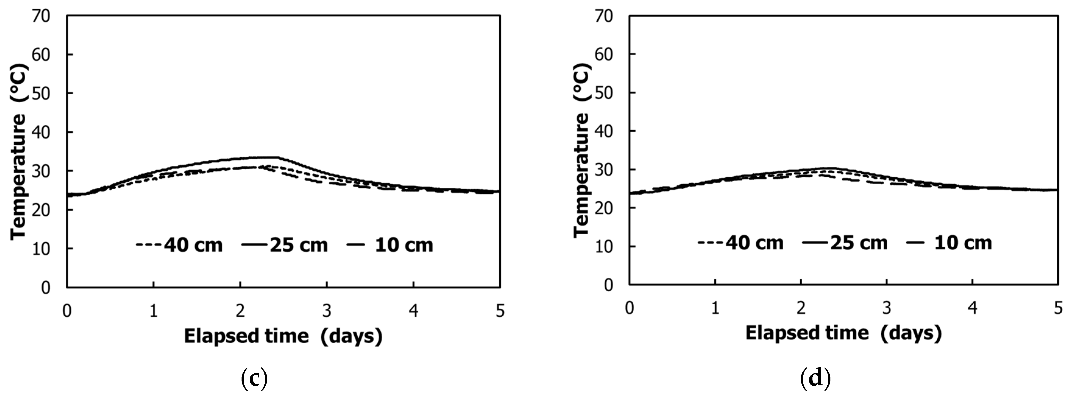
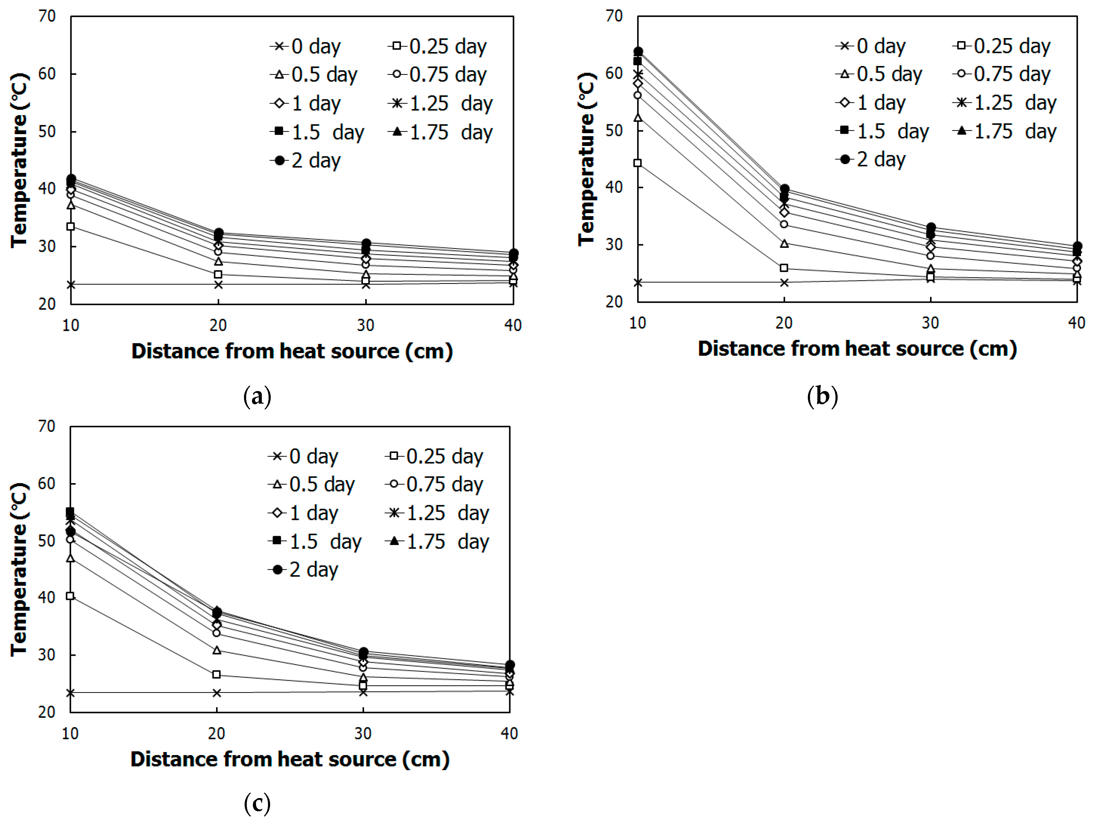
Figure 5 shows the experimental results of temperature changes in horizontal distances from the heat source. The temperature change from the heat source was larger than the 10 cm point at 20 cm depth in the ground and increased up to maximum 64.61 °C. The reason why the temperature change at 10 cm is small is that heat energy is lost due to the discharge of water vapor near the surface.

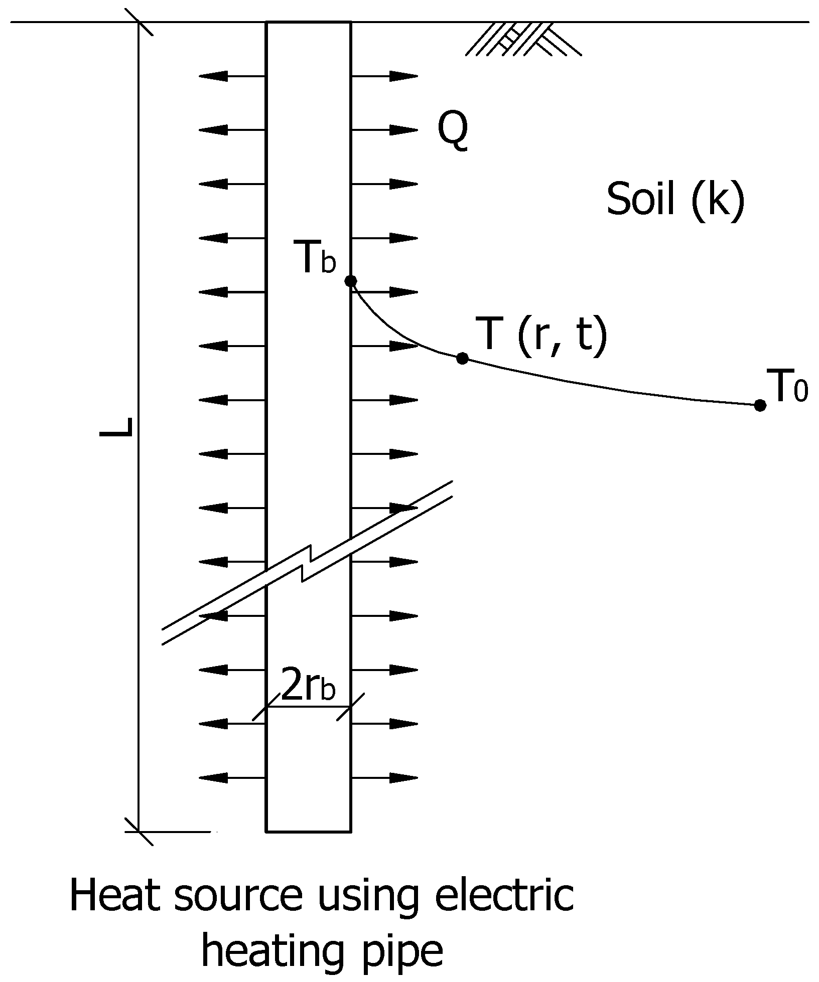
3.3. Linear Heat-Source Model (Case 1)

The analysis conditions of the linear heat-source model were as follows: the initial temperature ${\mathrm{T}}_0$ of 23.48 °C measured by the thermometer was set as a constant value, with $\mathrm{k}$ (thermal diffusivity) at 3.0 (W/m °C), with $\mathsf{\alpha }$ at 0.039744 (m²/day), and the heating calorific value, Q/L (specific heat-extraction rate), was applied at $925.0\left(\mathrm{W}/\mathrm{m}\right)$, which was the same as the direct current power-supply device. The radii of 10–40 cm were set as variables (

Table 1. Input data of linear heat-source model shown in Equation (7).

${\mathbf{T}}_0$	Q/L (W/m)	$\mathbf{k}$ $\left(\mathbf{W}/\mathbf{m}·\mathbf{K}\right)$	$\mathbf{r} \left(\mathbf{m}\right)$	$\mathbf{p}\mathbf{c}$ (kcal/m3 K)	A (m2/day)
23.48	925	3	0.1, 0.2, 0.3, 0.4	2160	0.039744

).

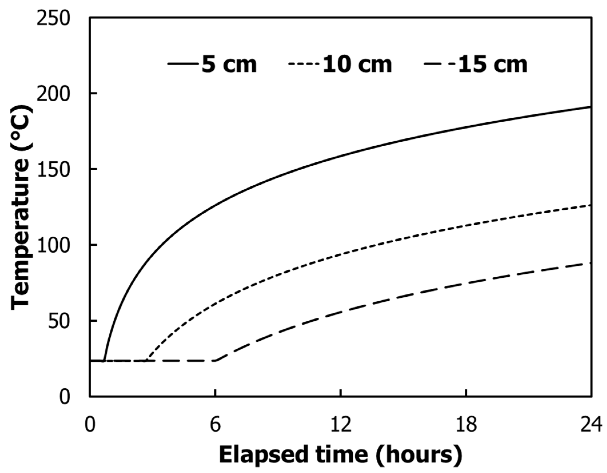
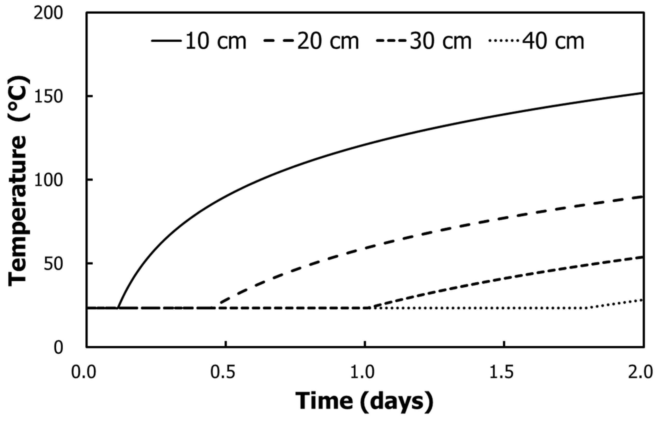
Figure 6 shows the results of comparison of temperature changes over time by the linear heat-source model. At a point 10 cm away from the heat source in the horizontal direction, a temperature change occurred after about 4 h, and increased to about 150 degrees. The temperature increased to about 100 degrees at a distance of 20 cm.

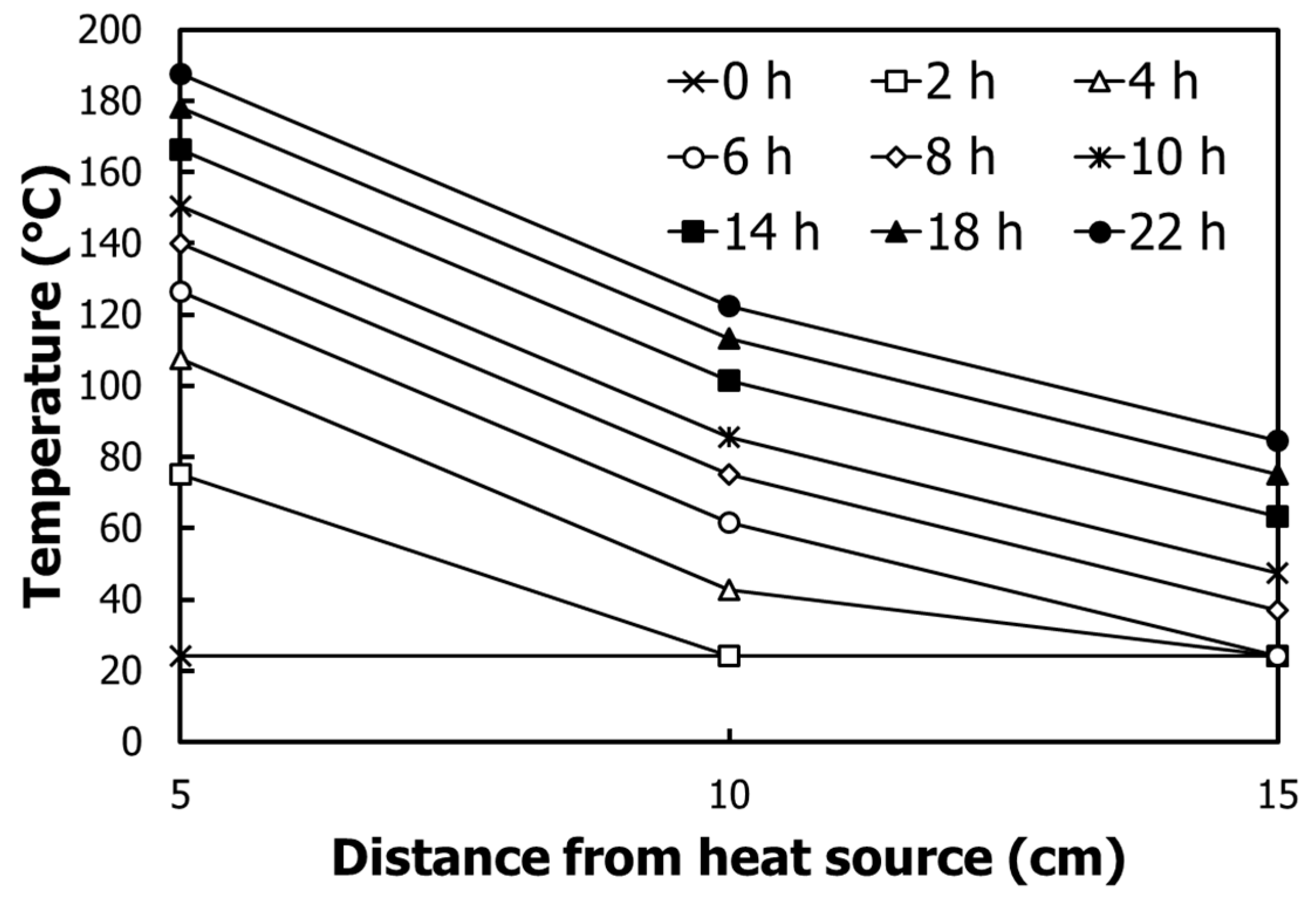
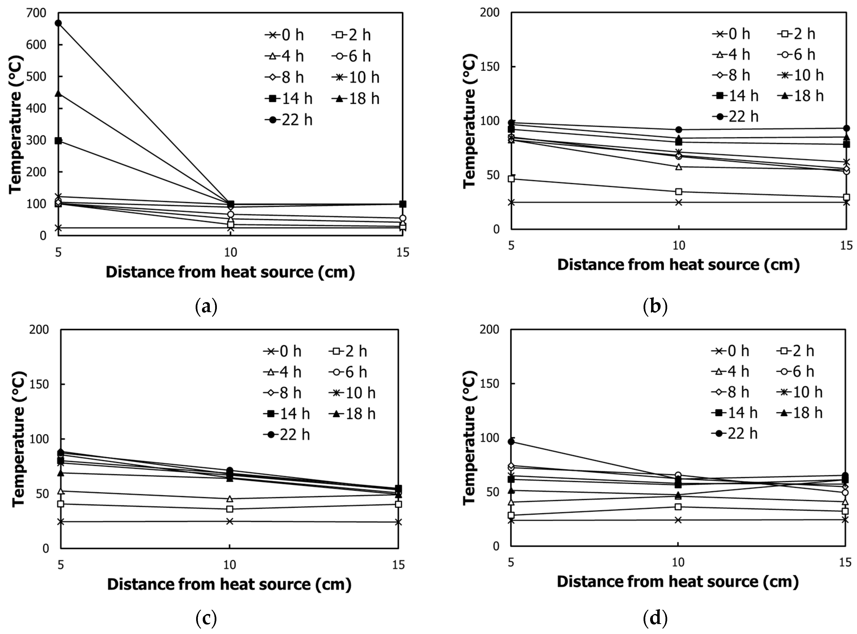
Figure 7 shows the temperature changes according to horizontal distances from the heat source by the linear heat model. According to the analysis results, the spots $10\mathrm{cm}$ away showed the maximum temperature increase of $164.13$ degrees, while that 20 cm away had the maximum temperature increase of $99.14$ degree; $30\mathrm{cm}$ ($61.11$ degree); and $40\mathrm{cm}$ ($34.14$ degree).

3.4. Numerical Analysis Model (Case 1)

In this section, the temperature changes due to the ground heating are estimated by numerical analysis. Heat transfer in the ground, which consists of soil particles, voids and pore water, is caused by conduction of soil particles and pore water. The ground is a porous material and convection heat transfer does not occur. Because the amount of pore water depends on the soil water content, seepage analysis must be conducted before heat-transfer analysis. Seepage analysis and heat-transfer analysis were conducted by SEEP/W and TEMP/W of GEO-SLOPE International Ltd., Calgary, AB, Canada. The seepage analysis was performed using the SEEP/W to estimate the distribution of pore water pressure and water content, and the TEMP/W was used for the heat-transfer analysis. TEMP/W is a finite-element software product that can be used to model the thermal changes in the ground due to environmental changes, or due to the construction of facilities, such as buildings or pipelines. The comprehensive formulation makes it possible to analyze both simple and highly complex geothermal problems, with or without temperatures that result in freezing or thawing of soil moisture [20].

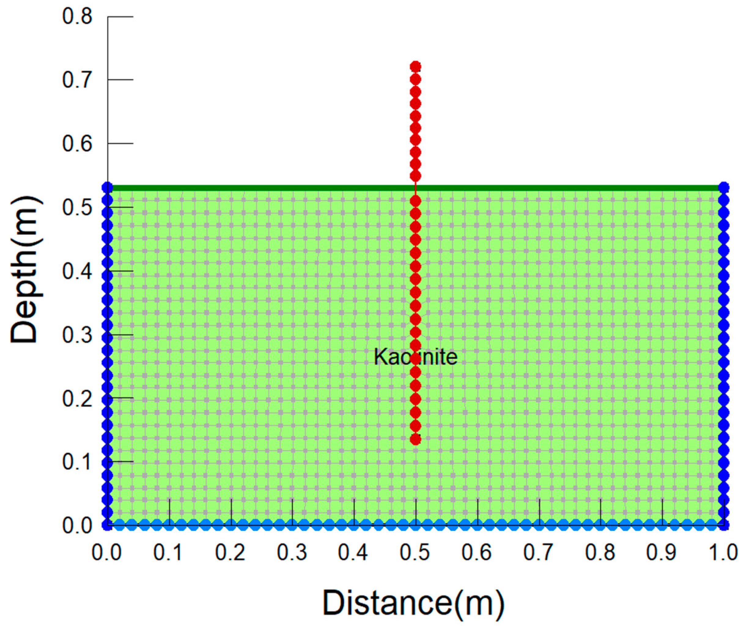
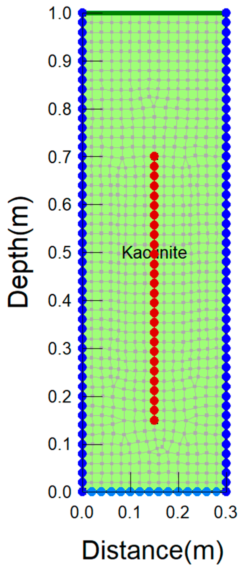
Figure 8 shows the numerical model applied to heat-transfer analysis (case 1). The cross-section of the numerical analysis model is the same as the cross-section of the experiment in Figure 3. The mesh size is 0.02 m, considering the electrical conductivity and the analysis time. The initial conditions and the boundary conditions of the numerical model were applied to the temperature measured in the experiment. Firstly, the initial temperature of kaolinite is 22.75 °C, and the temperature of the interface of the soil box is 23.48 °C. In Figure 8, the nodes at the left and right boundaries are blue circle, and the bottom is sky blue circle. The temperature of the electric heating pipe, which is a heat source, is $925\mathrm{W}/\mathrm{m}$ of electric power supplied from the DC power supplier, and the surface heating temperature is 500 °C. In Figure 8, it is a red circle.

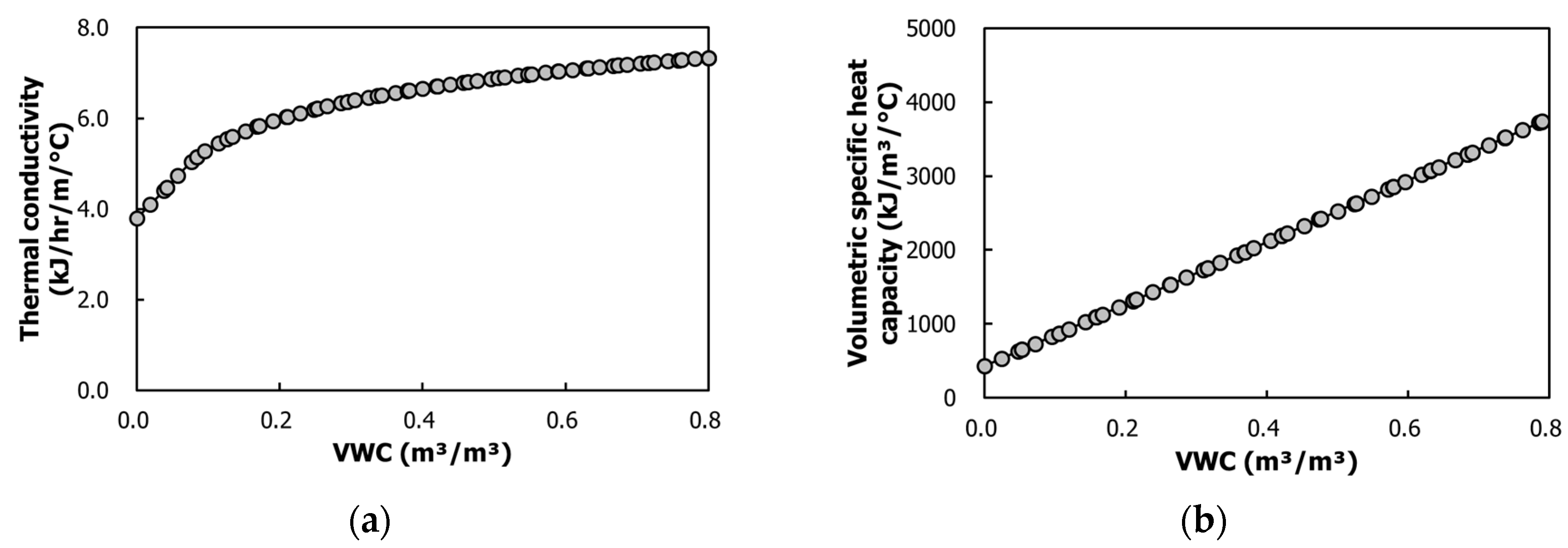
The physical properties of the soil required for heat-transfer analysis are the two curves shown in Figure 9. Figure 9a shows a function between the volumetric water content (VWC) and heat conductivity. Figure 9b is a function of the optimal water content and specific volume. For material properties of the heat-transfer characteristics of the reference clay, kaolinite, this study used the literature values of Michot et al. [22].

In the analysis procedure, the water content of the clay was estimated by the seepage analysis, and the heat-transfer analysis was carried out with the initial conditions. The water content of the soil was applied in the same saturated condition as the experimental conditions. In general, seepage analysis of the soil is performed in steady state and associated unsteady state. However, since the kaolinite used in the experiment has a very small coefficient of permeability, no flow of pore water was observed during the heating experiment. Therefore, the unsteady state analysis was not performed, and the results of the steady-state analysis were applied as the initial conditions of the heat-transfer analysis.

3.5. Comparison and Discussion (Case 1)

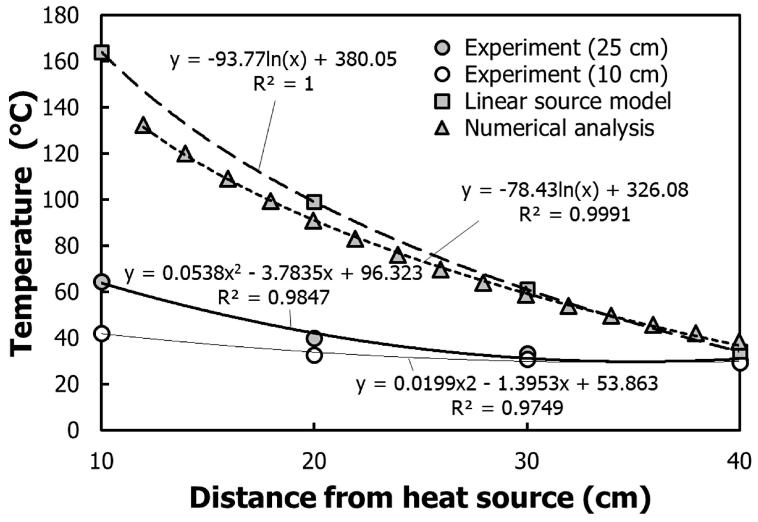
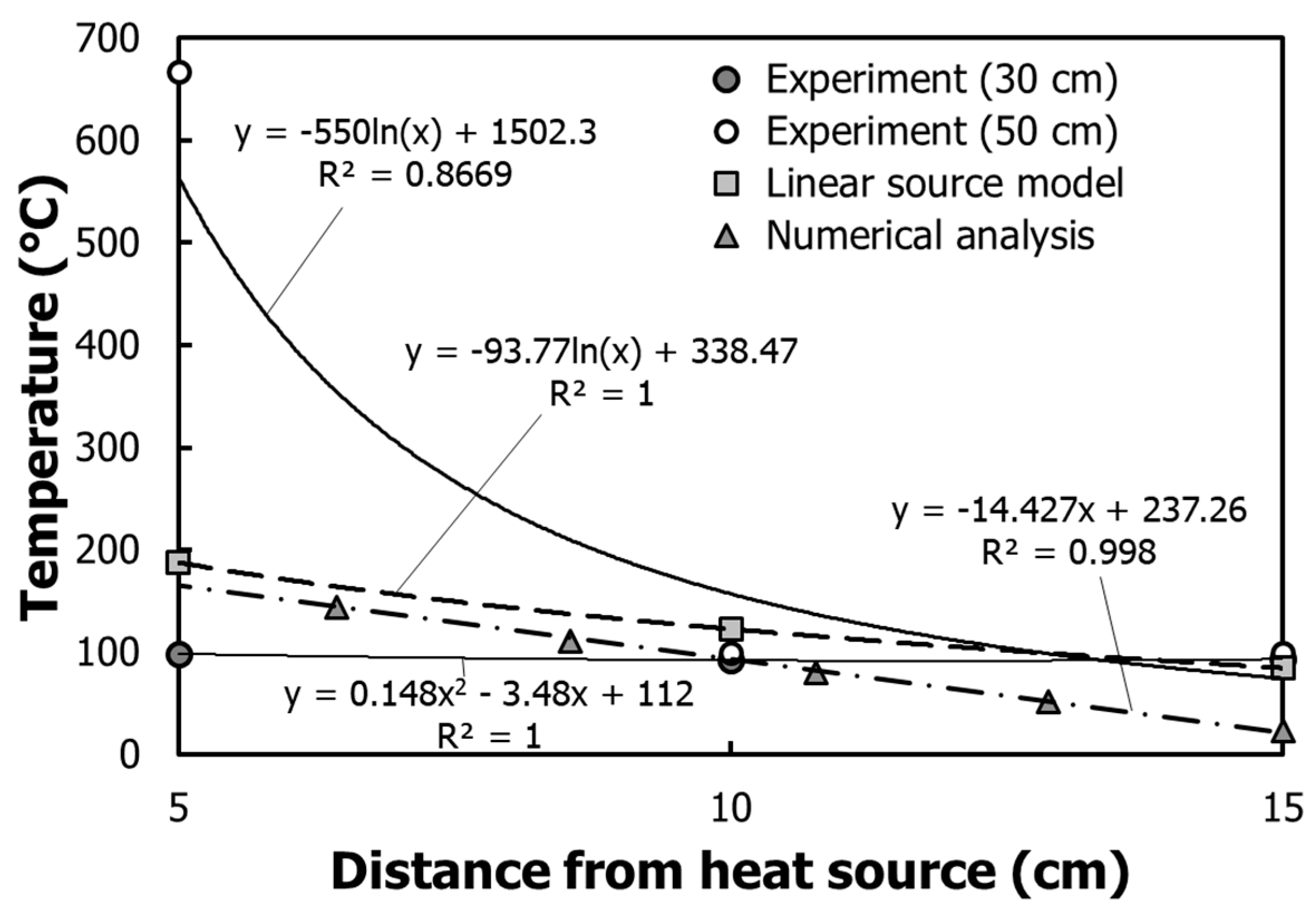
Figure 10 shows the results of comparison between the linear heat-source model, numerical analysis and the experiment results. Temperature changes according to horizontal distances from the heat source were observed after two days of ground heating. The linear heat-source model showed the highest temperature difference, followed by the numerical analysis and the experiment. The experiment showed the lowest temperature, due to heat loss by water-vapor discharge. The analysis of temperature changes in a horizontal direction from the heat source showed the results in a quadratic function form, and the linear heat-source model and the numerical analysis showed a constant decrease. Because of the increased loss of heat energy due to the discharge of water vapor near the surface, the temperature change was 25 cm higher than the 10 cm depth.

In this section, the electric heating test was conducted by allowing vapor generated by heating to be discharged. According to the temperature measurements, the end of the electrical heating (30 cm underground) showed the smallest horizontal temperature change. This indicates that heat transfer occurs more actively in a vertical direction than in a horizontal direction. Also, those spots 25 cm underground had greater temperature changes than those spots underground by 10 cm, which can be ascribed to heat losses due to vapor discharge.

According to the comparative analysis results with the linear heat-source model, the experimental results (64.6 °C) revealed a smaller temperature change than the linear heat-source model. This is believed to be due to heat loss as vapor was discharged to the surface. Also, the linear heat-source model showed a temperature decrease in a logarithmic function form along the horizontal distances, whereas the experimental results showed a decline in the form of a second-degree polynomial function.

4. Characteristics of Heat Transfer Due to Vapor-Discharge Suppression

4.1. Ground Heating and Measurement System (Case 2)

For the experiment with vapor-discharge suppression, the soil box with a height of 100 cm and a diameter of 30 cm was used. In order to suppress vapor generated by heating from being discharged by the self-weight consolidation of the standard clay, an electrical heating pipe with a height of 58.5 cm was interpenetrated 30 cm underground. Thermometers were positioned in the horizontal direction at a 5 cm interval in three rows and positioned in the vertical direction in four columns at the middle point of the electrical heating pipe (50 cm underground), at the upper end (30 cm underground), at 10 cm above the upper end (20 cm underground), and at 20 cm above the upper end (10 cm underground) (Figure 11).

In the experiment with vapor-discharge suppression, the electric current of 185 A with a resistance of 5 Ω was consumed at a rate of about 925 W per hour, and the surface temperature of the heat source by the electric energy was 500 °C, the same as the above experiment. In about 22 h of heating, the surrounding temperature was increased to more than 600 °C, and the power supply line of the electric heating pipe was disconnected, leading to the termination of the electric heating.

4.2. Temperature Measurement Results (Case 2)

Figure 12 shows the temperature changes depending on horizontal distances from the heat source according to underground depths. Figure 12a shows the temperature changes at the middle point of the electric heating pipe or at 50 cm underground. Figure 12b shows the temperature changes at the upper end of the electric heating pipe, or at 30 cm underground. Figure 12c shows the temperature changes at 10 cm above the upper end of the electric heating pipe, or at 20 cm underground. Figure 12d shows the temperature changes at 20 cm above the upper end of the electric heating pipe, or at 10 cm underground.

Each graph shows that those spots 5 cm away from the heat source in the horizontal direction had rapid temperature changes due to vapor. This phenomenon is due to the fact that the vapor had not been discharged until a certain pressure, and then was suddenly emitted to the surface at a higher pressure; the temperature dropped sharply after the discharge.

Figure 13 shows the temperature changes depending on underground depths according to horizontal distances. Figure 13a shows the temperature changes depending on underground depths at a horizontal distance of 5 cm from the heat source, Figure 13b at a horizontal distance of 10 cm, and Figure 13c at a horizontal distance of 15 cm. The middle point of the electric heating pipe (50 cm underground) showed a rapid temperature increase to up to 718.8 °C. The experiment with vapor-discharge suppression had relatively greater temperature changes in 22 h of heating than the experiment with vapor discharge, and showed temperature increases of about 60–100 °C. The irregular temperature-change curve means that vapor was moved to the surface in an irregular way. Also, in case of vapor-discharge suppression, heat transfer by vapor occurred, increasing the temperatures at all underground depths by less than 100 °C.

Figure 14 shows the temperature changes depending on underground depths by horizontal distances from the heat source. The experimental results showed smaller temperature changes than the linear heat-source model. Also, the middle point of the electric heating pipe showed remarkably high-temperature differences along the horizontal distances, and revealed a dwindling temperature difference according to the horizontal distance as it went up higher above the end of the electric heating pipe.

4.3. Linear Heat-Source Model (Case 2)

The linear heat-source model had the same analysis conditions as the vapor discharge experiment, and thermometers were positioned within the radii of 5–15 cm, which was set as the variable measurement.

Figure 15 shows temperature changes over time by horizontal distances from the heat source. Those spots 5 cm away from the heat source revealed a temperature change in about 30 min of heating; those 10 cm away in about 2.5 h; and those 15 cm away in about 6 h.

Figure 16 shows temperature changes by horizontal distances from the heat source. According to the analysis results, the temperatures of the spots 5 cm away from the heat source increased to the maximum of 187.55 degree; 10 cm away to 122.55 degree; and 15 cm away to 84.53 degree.

4.4. Numerical Analysis Model (Case 2)

Figure 17 shows the numerical model applied to heat-transfer analysis (case 2). The cross-sectional shape of the model is shown in Figure 11. The mesh, boundary condition, and analysis procedure of the numerical model are the same as in case 1. The temperature of the boundary condition of the model was applied to the measured value in case 2. The mesh size is 0.02 m, considering the electrical conductivity and the analysis time. The initial conditions and the boundary conditions of the numerical model were applied to the temperature measured in the experiment. Firstly, the initial temperature of kaolinite is 23.79 °C, and the temperature of the interface of the soil box is 24.71 °C. In Figure 8, the nodes at the left and right boundaries are blue circle, and the bottom is sky blue circle. The temperature of the electric heating pipe, which is a heat source, is $925\mathrm{W}/\mathrm{m}$ of electric power supplied from the DC power supplier, and the surface heating temperature is 500 °C. In Figure 17, it is a red circle. The properties of kaolinite were applied to the graph of Figure 9 as in case 1. In the analysis step, seepage analysis of the steady-state condition was performed first, and heat-transfer analysis was performed with the result as an initial condition.

4.5. Comparison and Discussion (Case 2)

In this section, the temperature measurement results of the electric heating experiment carried out under the restrained discharge condition of water vapor are compared to temperature changes estimated by the theoretical solution of the linear heat-source model and by the numerical analysis. The physical properties applied by the numerical analysis are the same as in Section 3.5.

Figure 18 shows temperature changes in 22 h of heating by horizontal distances from the heat source. At a depth of 30 cm above 5 cm in the vertical direction from the heat source, the highest temperature change occurred, and increased to a maximum of 667.6 °C. This result is caused by the heat transfer by water vapor, because clay with a small permeability does not generate the flow of pore water. The temperature increased only up to about 100 °C at 50 cm, which is the same depth as the heat source. As a result, the heat transfer of the saturated clay was shown to be transmitted more vertically by water vapor than in the horizontal direction. Unless water vapor caused loss of heat energy, the experiment showed larger temperature change than the linear heat-source model and numerical analysis.

5. Discussion and Summary

The purpose of this study is to investigate the heat-transfer characteristics of water vapor generated by ground heating. In this study, experiments were carried out according to whether or not the water vapor generated by the ground heating was discharged. The linear heat-source model and the numerical analysis, which were used to estimate the temperature distribution of the ground, were performed and compared with the experimental results. The results of this study are summarized and discussed as follows.

As a result of measuring the temperature change when the water vapor was discharged, the largest temperature change occurred at the point where the electric heating tube was installed. The temperature change was small when it was close to the ground surface. This is because the water vapor generated from the bottom continuously increases the temperature in the vertical direction and is discharged as water vapor on the surface. The linear heat source model and the numerical analysis were evaluated more than the experiment under the condition that the discharge of water vapor was suppressed.

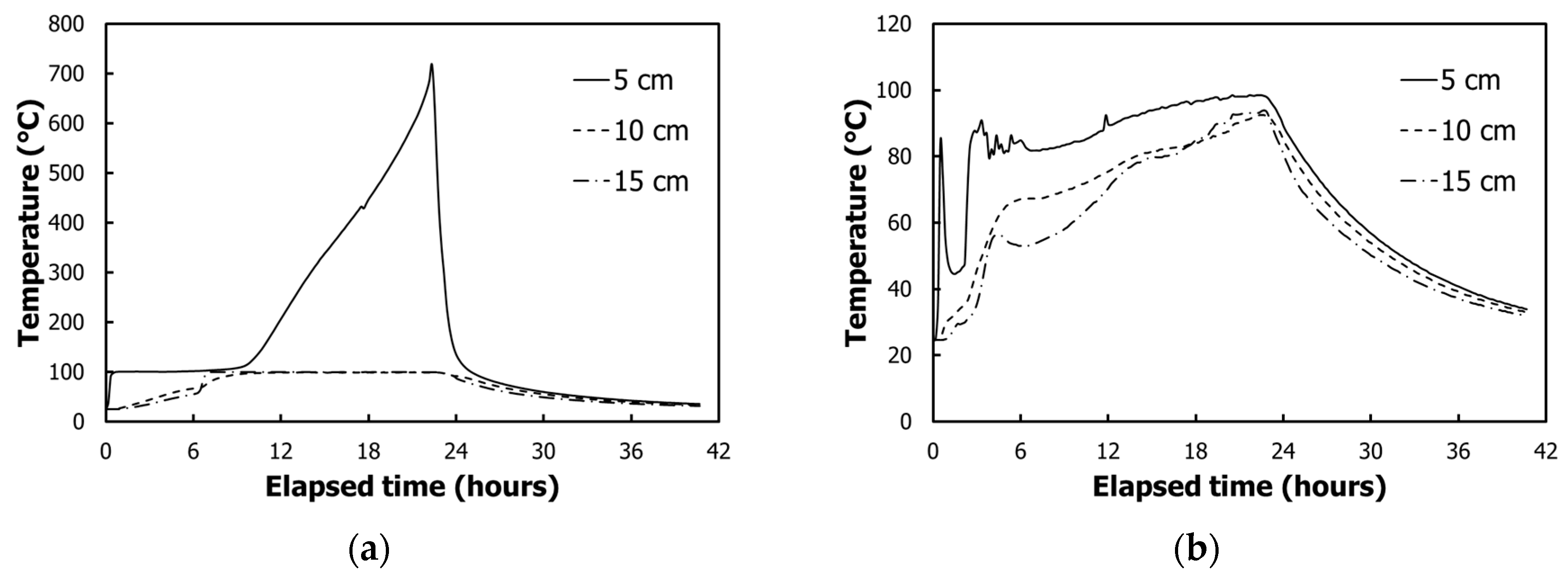
As a result of experiments under the condition that water vapor is not discharged, At the top 5 cm of the electric heating pipe, The soil temperature increased up to 718.8 degrees, which is higher than 500 degrees of the heat source. In addition, the temperature change in the vertical direction was larger than that in the horizontal direction. And, heat transfer due to water vapor was found to have a great influence. When heat transfer due to water vapor occurred, the temperature change was larger than the linear heat-source model and numerical analysis. Conversely, if no heat transfer occurred, the temperature change was small.

The linear heat-source model estimates the one-dimensional soil temperature change from the heat source. Although it is suitable for an underground heat exchanger where the heat source is infinitely long and the heat flux is constant, it is not suitable for the ground-heating method. Numerical analysis considers only two-dimensional heat transfer by conduction of soil particles and pore water, but does not consider the phase-change energy and heat transfer by water vapor.

6. Conclusions

In this study, the electric heating experiment was performed and compared with theoretical and numerical results. The conclusions of this study are as follows:

• The heat-transfer properties of the saturated ground changed according to the presence and absence of water vapor discharged by heating. If water vapor was discharged, the temperature dropped dramatically due to heat loss. To apply the ground-heating method to actual field sites, it is necessary to restrain the discharge of water vapor, as reported by Park, Lee, Jang and Han [2].
• The theoretical solution and the numerical analysis method applied to the design of the ground heat exchanger were used to calculate the temperature change by the ground heating. Compared with the conditions in which the water vapor was discharged, many differences appeared. This is because the phase change of the pore water and the heat-transfer process of the water vapor were not considered.
• To commercialize the soft ground improvement by ground heating, it is necessary to develop a theoretical solution and a numerical analysis model that can estimate the ground-heat transfer phenomenon due to water vapor. In the field, the discharge of water vapor is suppressed depending on the installation depth of the electric heating pipe. This is because the self-weight of the soil suppresses the vapor pressure of the water vapor. Further research on this process is needed.
• The ground-heating method using electric energy developed by this study turned out be effective in preventing the environmental degradation and ensuring a sustainable development of mud flats compared with the previous techniques. Therefore, continuous related studies and efforts to improve the related technique are needed.

References

1. Park, M.-C.; Im, E.-S.; Shin, B.-C.; Han, H.-S. Improvement of shallow soil using electric heating equipment. J. Korean Geotech. Soc. 2012, 28, 41–54. [Google Scholar] [CrossRef]
2. Park, M.; Lee, K.; Jang, J.; Han, H. Thermal Analysis of Silty Sand Soil by Pipe Heater Installed in the Ground. J. Korean Geoenviron. Soc. 2013, 14, 5–13. [Google Scholar]
3. Beles, A.; Stănculescu, I. Thermal treatment as a means of improving the stability of earth masses. Geotechnique 1958, 8, 158–165. [Google Scholar] [CrossRef]
4. Litvinov, I.M. Stabilization of Settling and Weak Clayey Soils by Thermal Treatment; Highway Research Board: Washington, DC, USA, 1960; pp. 94–112. [Google Scholar]
5. Wintermyer, A. Percentage of water freezable in soils. Public Roads 1925, 5, 5–8. [Google Scholar]
6. Van der Lingen, G.; Biesenbach, J. Investigations on the heat treatment of subsoils and gravels. South African Ind. Chem. 1949, 3, 70–74. [Google Scholar]
7. Bose, S.K. Stabilization of Certain Clayey Soils in India by Thermal Treatment. J. Indian Road Congr. 1953, 18. [Google Scholar]
8. Chandrasekharan, E.C.; Boominathan, S.; Sadayan, E.; Narayanaswamy, S.K. Influence of Heat Treatment on the Pulverization and Stabilzation Characteristics of Typical Tropical Soils; Highway Research Board: Washington, DC, USA, 1969; pp. 161–172. [Google Scholar]
9. Wang, M.C.; Benway, J.M.; Arayssi, A.M. The effect of heating on engineering properties of clays. In Physico-Chemical Aspects of Soil and Related Materials; STP 1095; ASTM: Philadelphia, PA, USA, 1990; pp. 1139–1158. Available online: https://www.astm.org/DIGITAL_LIBRARY/STP/PAGES/STP23553S.htm (accessed on 30 January 2018).
10. Lambe, T.W. A mechanistic picture of shear strength in clay. In Proceedings of the Research Conference on Shear Strength of Cohesive Soils, Boulder, CO, USA, June 1960; ASCE: New York, NY, USA, 1960; pp. 555–580. Available online: http://cedb.asce.org/CEDBsearch/record.jsp?dockey=0138193 (accessed on 30 January 2018).
11. Litvinov, I.; Rzhanitzin, B.; Bezruk, V. Stabilization of soil for Constructional Purposes. In Proceedings of the Fifth International Conference on Soil Mechanics and Foundation Engineering, Paris, France, 17–22 July 1961; pp. 775–777. [Google Scholar]
12. Park, M.-C.; Im, E.-S.; Lee, K.-S.; Han, H.-S. Experimental Study for Consolidation by Electric Heating Systems. J. Korean Geoenviron. Soc. 2012, 13, 43–53. [Google Scholar]
13. Spilker, E.H. Ground-coupled heat pump loop design using thermal conductivity testing and the effect of different backfill materials on vertical bore length. Ashrae Trans. 1998, 104, 775. [Google Scholar]
14. Alfaro, M.C.; Ciro, G.A.; Thiessen, K.J.; Ng, T. Case study of degrading permafrost beneath a road embankment. J. Cold Reg. Eng. 2009, 23, 93–111. [Google Scholar] [CrossRef]
15. Kersten, M.S. Laboratory Research for the Determination of the Thermal Properties of Soils; Minnesota University Minneapolis Engineering Experiment Station: Minneapolis, MN, USA, 1949. [Google Scholar]
16. Manohar, K.; Yarbrough, D.W.; Booth, J.R. Measurement of apparent thermal conductivity by the thermal probe method. J. Test. Eval. 2000, 28, 345–351. [Google Scholar]
17. Kelvin, L.; Thomson, W. Mathematical and Physical Papers: Collected from Differnet Scientific Periodicals from May, 1841, to the Present Time; Cambridge University: Cambridge, UK, 1890; Volume 3, 529p. [Google Scholar]
18. Carslaw, H.S.; Jaeger, J.C. Conduction of Heat in Solids, 2nd ed.; Clarendon Press: Oxford, UK, 1959. [Google Scholar]
19. Segerlind, L.J. Applied Finite Element Analysis; John Wiley & Sons Inc.: Hoboken, NJ, USA, 1984. [Google Scholar]
20. Krahn, J. Thermal Modeling with TEMP/W: An Engineering Methodology, 2014 ed.; GEO-SLOPE International, Ltd.: Calgary, AB, Canada, 2004. [Google Scholar]
21. Kanthal, A.B. Heating Alloys for Electronic Household Appliances; Kanthal: Hallstahammar, Sweden, 2003. [Google Scholar]
22. Michot, A.; Smith, D.S.; Degot, S.; Gault, C. Thermal conductivity and specific heat of kaolinite: Evolution with thermal treatment. J. Eur. Ceram. Soc. 2008, 28, 2639–2644. [Google Scholar] [CrossRef]
Figure 1. The boundary condition of vertical heat exchanger.
Sustainability 10 00412 g001
Figure 2. Ground heating system. (a) Electric heating pipe; (b) DC power supplier; (c) resistance temperature detector (RTD).
Sustainability 10 00412 g002
Figure 3. Experimental setup of the emission case of water vapor. (a) Sectional view; (b) overall view.
Sustainability 10 00412 g003
Figure 4. Temperature variation according to ground depth; (a) 10 cm from the heat pipe; (b) 20 cm from the heat pipe; (c) 30 cm from the heat pipe; (d) 40 cm from the heat pipe.
Sustainability 10 00412 g004aSustainability 10 00412 g004b
Figure 5. Temperature variation according to horizontal distance from the heat pipe; (a) 10 cm (top of the heat pipe); (b) 20 cm (middle of the heat pipe); (c) 30 cm (bottom of the heat pipe).
Sustainability 10 00412 g005
Figure 6. Temperature variation according to elapsed time by linear heat model.
Sustainability 10 00412 g006
Figure 7. Temperature variation according to horizontal distance from the heat pipe by linear heat model.
Sustainability 10 00412 g007
Figure 8. Numerical model applied to heat-transfer analysis (case 1).
Sustainability 10 00412 g008
Figure 9. The heat-transfer characteristics of the soil applied to numerical analysis. (a) Volumetric water content (VWC) vs. thermal conductivity curve; (b) volumetric water content (VWC) vs volumetric specific heat capacity curve.
Sustainability 10 00412 g009
Figure 10. Comparison of temperature change from heat source (case 1).
Sustainability 10 00412 g010
Figure 11. Experimental setup of the emission suppression case of water vapor. (a) Sectional view; (b) overall view.
Sustainability 10 00412 g011
Figure 12. Temperature variation according to ground depth; (a) depth 50 cm; (b) depth 30 cm; (c) depth 20 cm; (d) depth 10 cm.
Sustainability 10 00412 g012aSustainability 10 00412 g012b
Figure 13. Temperature variation according to horizontal distance from the heat pipe; (a) 5 cm from the heat pipe; (b) 10 cm from the heat pipe; (c) 15 cm from the heat pipe.
Sustainability 10 00412 g013
Figure 14. Temperature variation according to ground depth; (a) depth 50 cm; (b) depth 30 cm; (c) depth 20 cm; (d) depth 10 cm.
Sustainability 10 00412 g014
Figure 15. Temperature variation according to elapsed time by linear heat model.
Sustainability 10 00412 g015
Figure 16. Temperature variation according to horizontal distance from the heat pipe by linear heat model.
Sustainability 10 00412 g016
Figure 17. Numerical model applied to heat-transfer analysis.
Sustainability 10 00412 g017
Figure 18. Comparison of temperature change from heat source (case 2).
Sustainability 10 00412 g018