Spatial Heterogeneity of Typical Ecosystem Services and Their Relationships in Different Ecological–Functional Zones in Beijing–Tianjin–Hebei Region, China


Abstract
1. Introduction
2. Background of the Study
3. Study Area and Materials
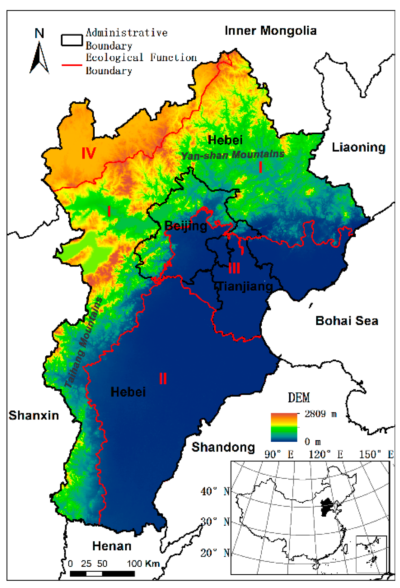
3.1. Study Area
3.2. Materials
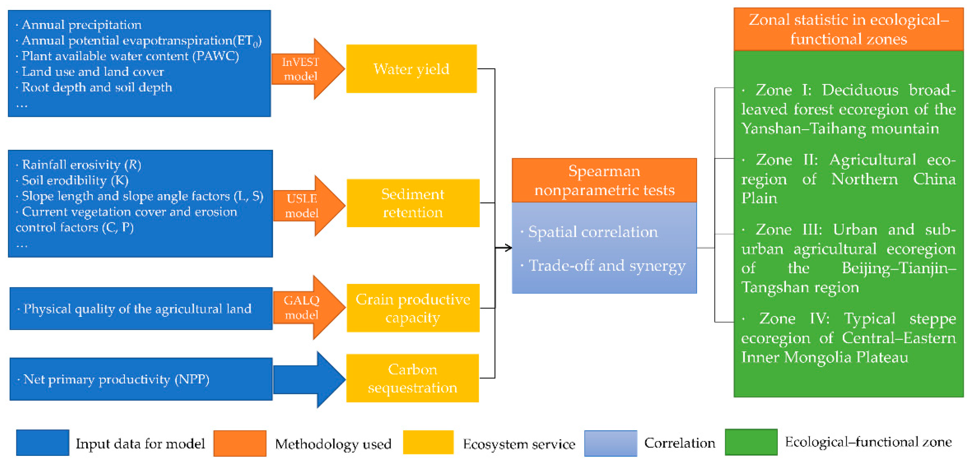
4. Methodology
4.1. Water Yield Assessment
4.2. Soil Retention Assessment
4.3. Grain Productive Capacity Assessment
5. Results
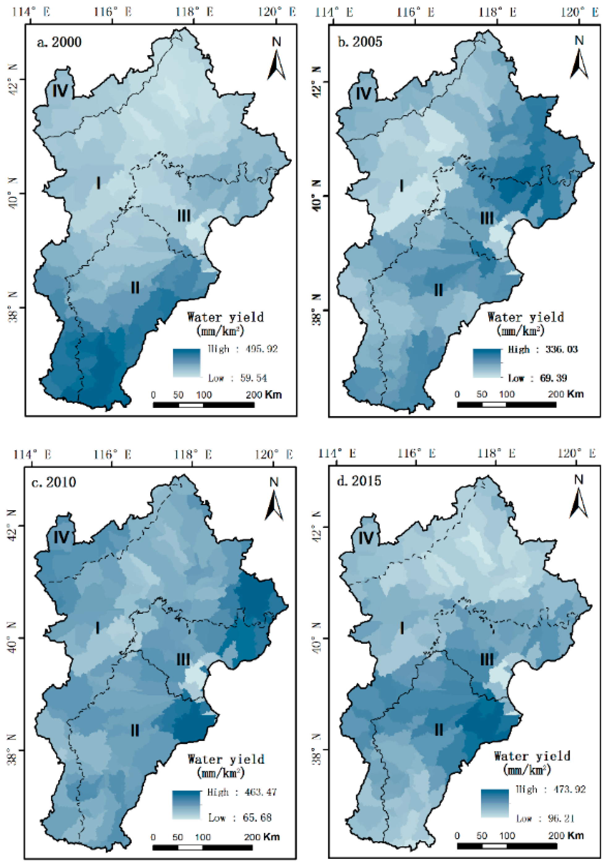
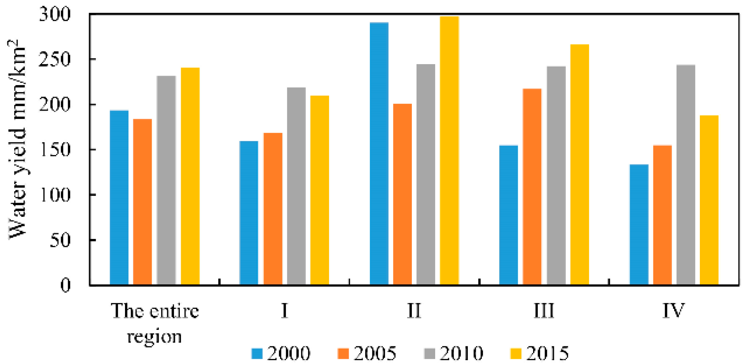
5.1. Water Yield
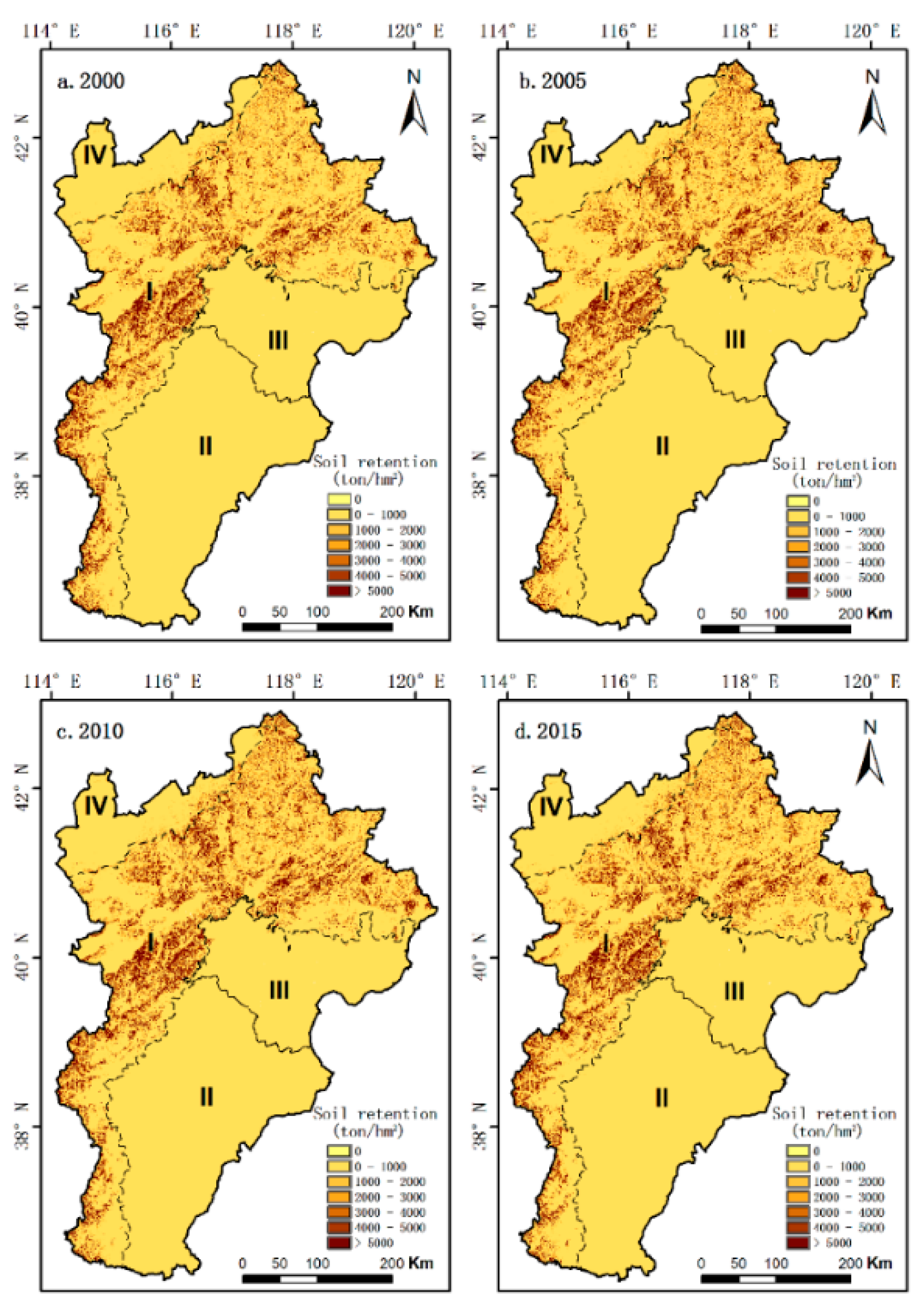
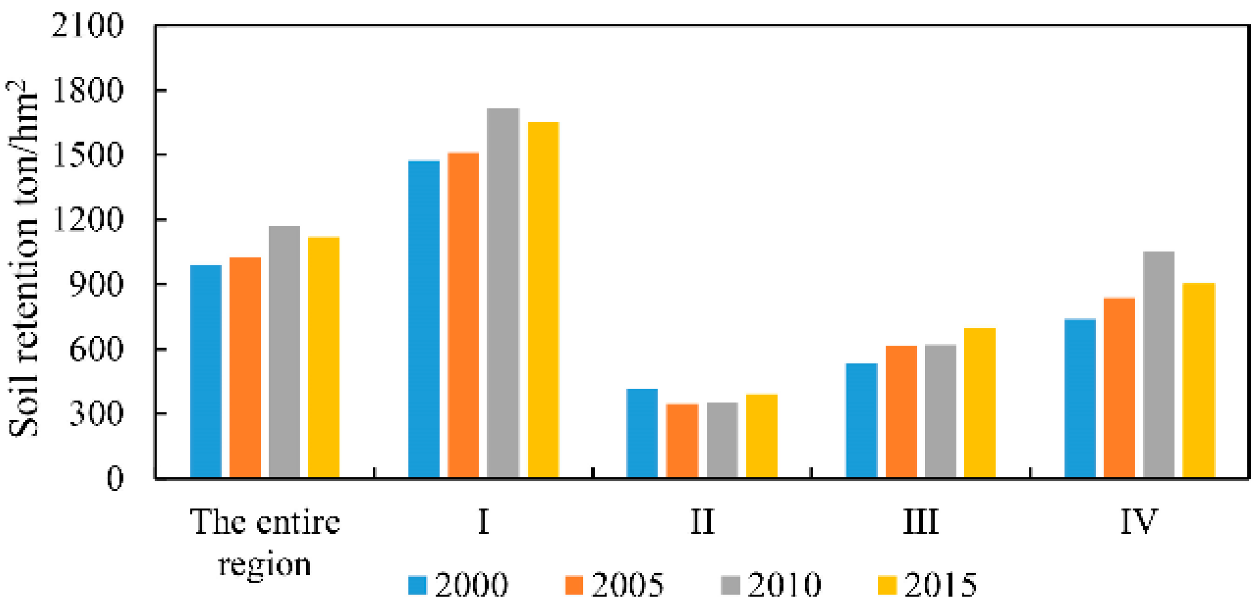
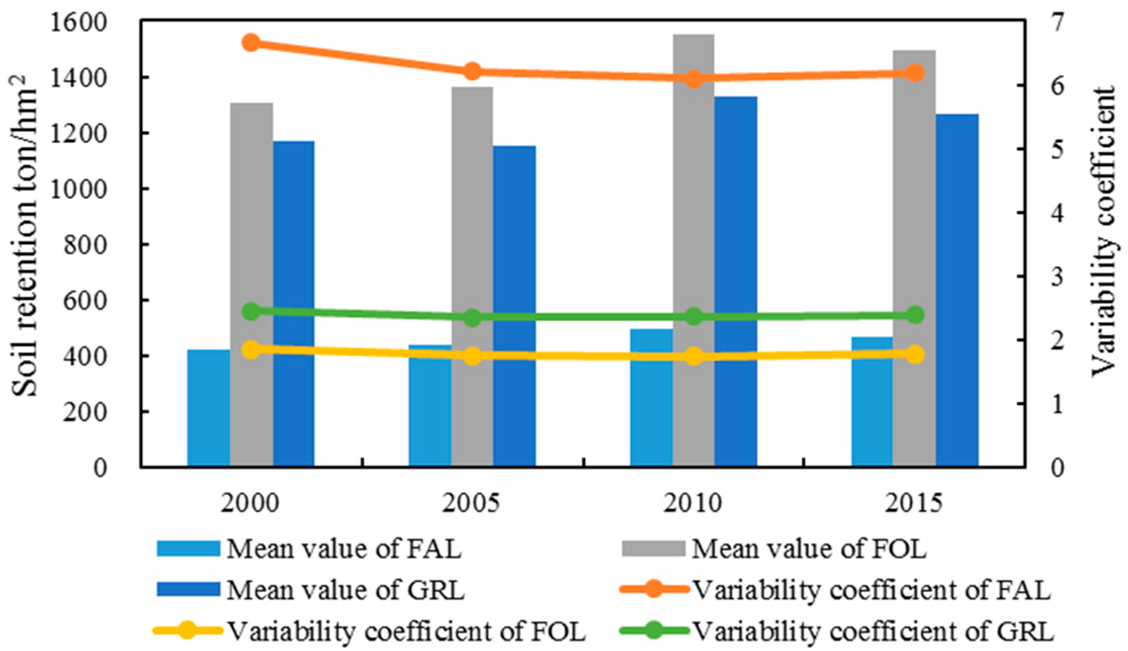
5.2. Sediment Retention
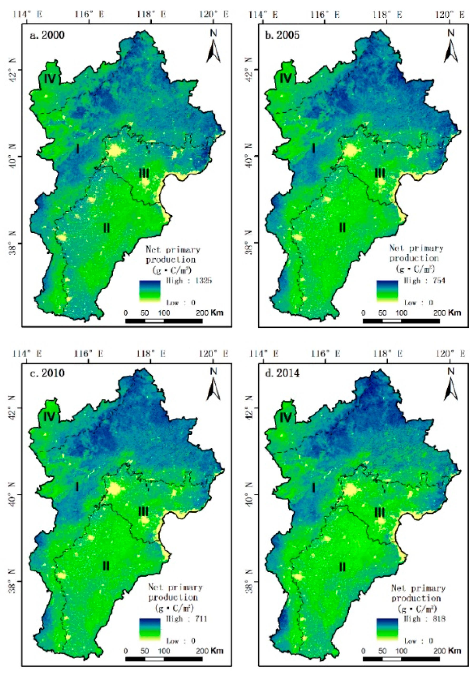
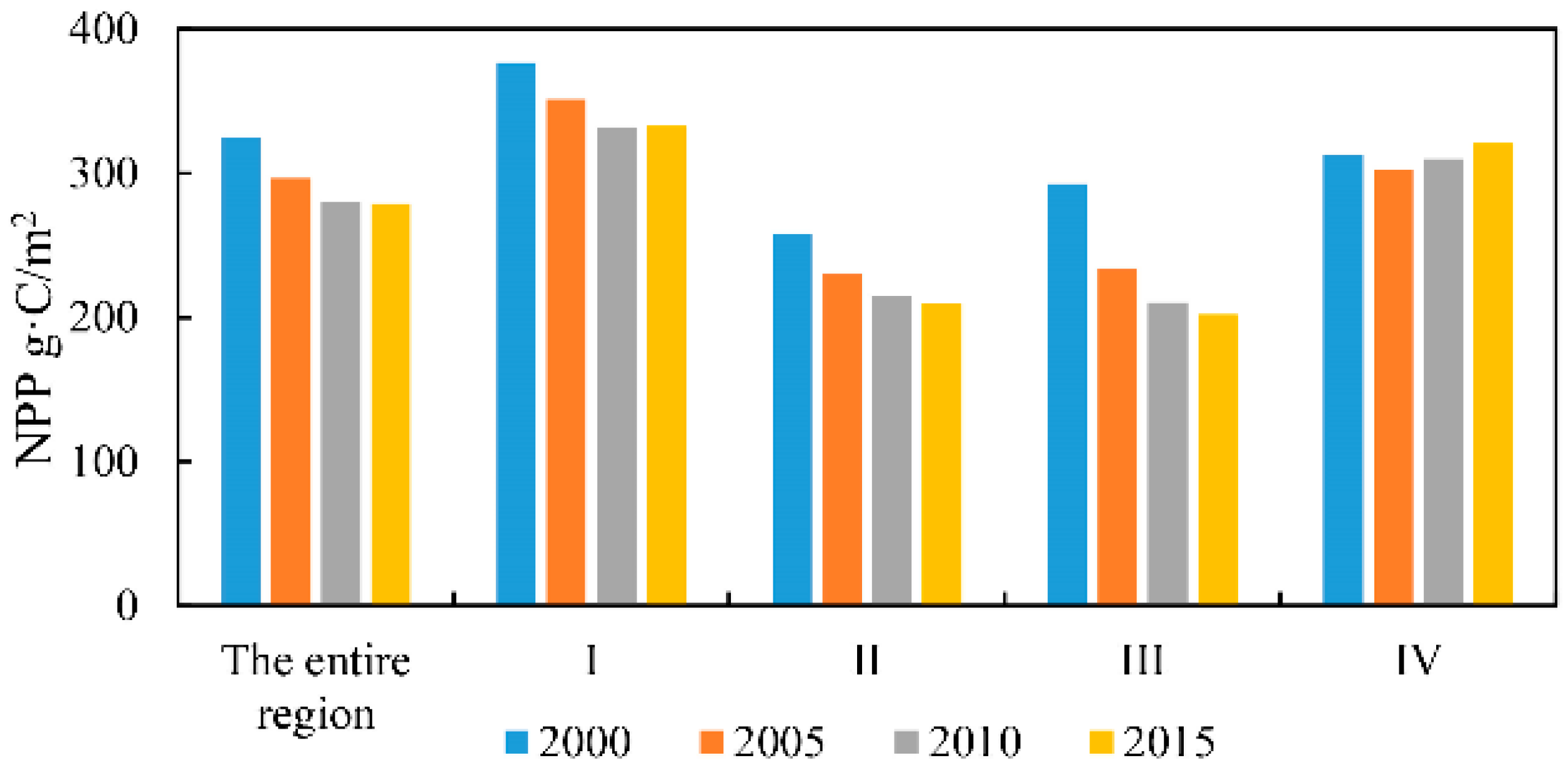
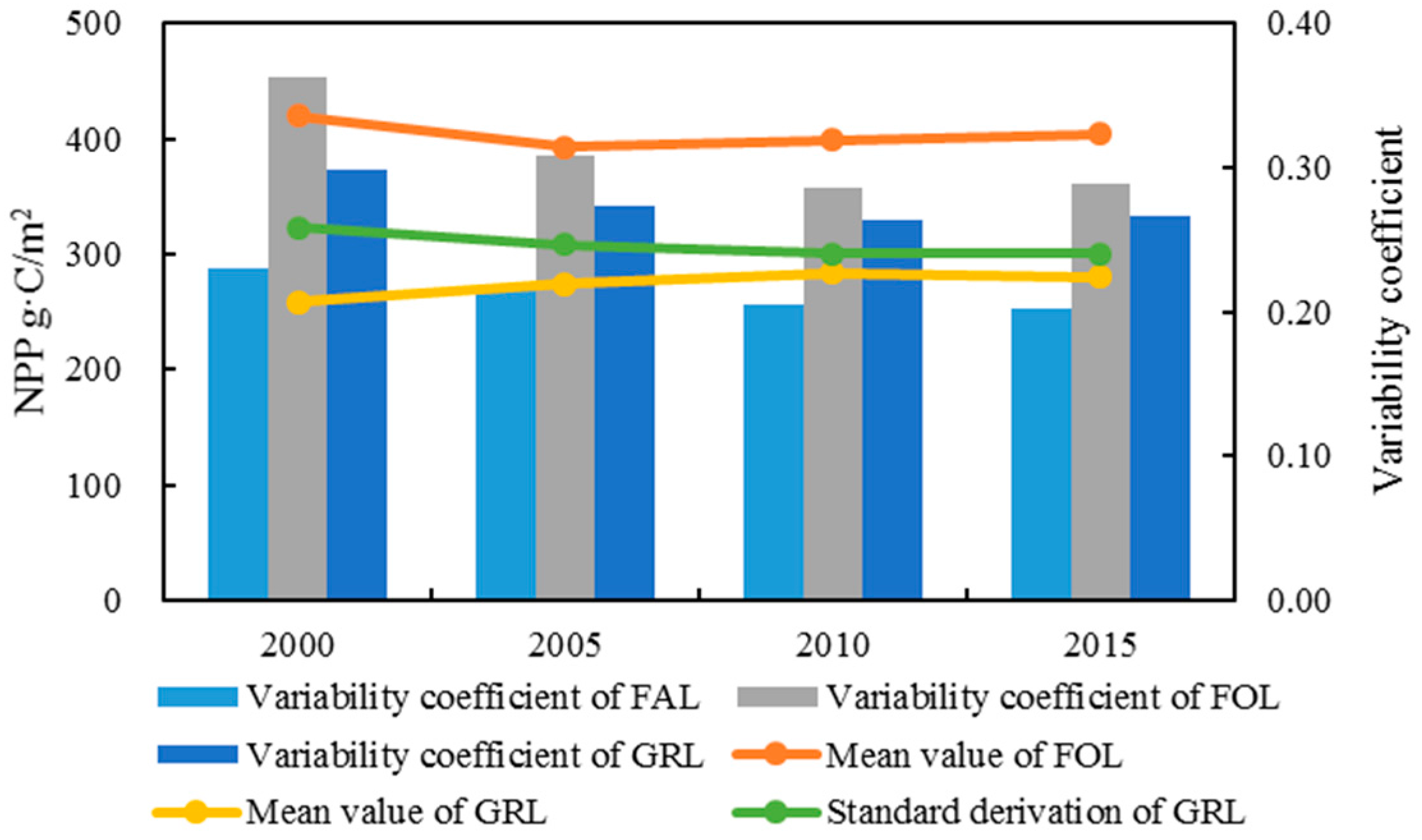
5.3. Carbon Sequestration
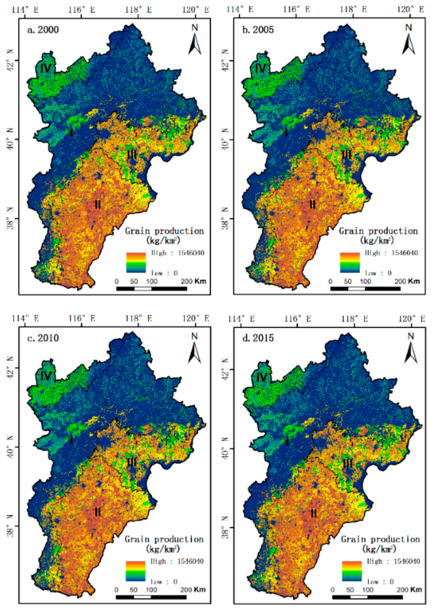
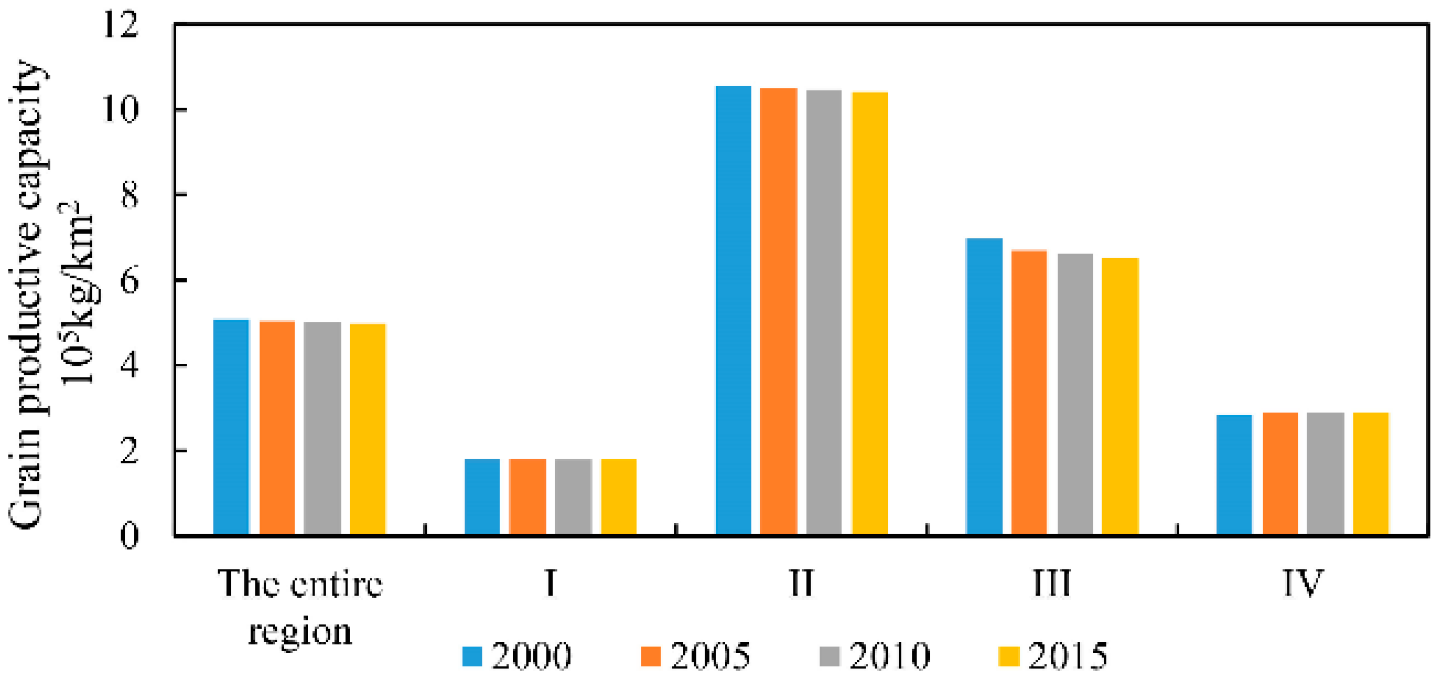
5.4. Grain Productive Capacity
5.5. Correlation among ES
6. Discussion
6.1. Impact of Land Use and Land Cover Change on ES
6.2. Correlative Mechanisms among ES
6.3. Implications for Regional Sustainable Development
6.4. Limitations
7. Conclusions
- The spatial distribution of water yield was relatively homogeneous but slightly high in Zones I, II and III and all increased generally each year. Sediment retention was high in Zones I and IV and low in Zones II and III. These values all gradually increased every year. The distribution of carbon sequestration was similar to that of soil retention but a downtrend occurred in the entire region rather than in Zone IV. High-quality farmland with high grain production was mainly distributed in Zones II and III and those in Zone III indicated a significant decline.
- Spearman correlation analysis indicated a positive spatial relationship between the status quo of water yield and soil retention/grain production capability/carbon sequestration, soil retention and carbon sequestration in the whole region. Furthermore, a positive relationship was observed between grain production capability and carbon sequestration in Zones II and III but a negative one was observed in Zones I and IV. A negative correlation was observed between grain production capability and soil retention in Zones I and IV. Regarding the relationship between trade-off and synergy, our results indicated synergies between soil retention and water yield/carbon and trade-offs between water yield and carbon sequestration/grain production in the whole region. In addition, grain production and carbon sequestration had synergy in Zones I and IV but trade-offs in Zone II and III. A weak trade-off was observed between grain production and soil retention only in Zone IV.
- The results of the transfer matrix demonstrated that encroachment on farmland occurred in the BTH region in 2000–2015, except for the grassland occupation by farmland in Zone IV. The government is suggested to implement sequentially the SLCP and prohibit reclamation and deforestation in Zone I. The authors emphasize the protection of high-quality farmland in Zone II to render it the “rice bag” of the BTH region. Furthermore, the farmland should be made multi-functional and its encroachment in Zone III should be prevented. Finally, the farmland should be returned for grass and grazing should be controlled in Zone IV to restore grassland ecology.
Acknowledgments
Author Contributions
Conflicts of Interest
References
- Costanza, R.; d’Arge, R.; de Groot, R.; Farber, S.; Grasso, M.; Hannon, B.; Limburg, K.; Naeem, S.; O’Neill, R.V.; Paruelo, J.; et al. The value of the world’s ecosystem services and natural capital. Nature 1997, 387, 253–260. [Google Scholar] [CrossRef]
- Millennium Ecosystem Assessment. Ecosystems and Human Well-Being: Current State and Trends: Synthesis; Island Press: Washington, DC, USA, 2005. [Google Scholar]
- Nelson, E.; Mendoza, G.; Regetz, J.; Polasky, S.; Tallis, H.; Cameron, D.R.; Chan, K.M.; Daily, G.C.; Goldstein, J.; Kareiva, P.; et al. Modeling multiple ecosystem services, biodiversity conservation, commodity production and tradeoffs at landscape scales. Front. Ecol. Environ. 2009, 7, 4–11. [Google Scholar] [CrossRef]
- Jiang, C.; Wang, F.; Zhang, H.; Dong, X. Quantifying changes in multiple ecosystem services during 2000–2012 on the Loess Plateau, China, as a result of climate variability and ecological restoration. Ecol. Eng. 2016, 97, 258–271. [Google Scholar] [CrossRef]
- Song, W.; Liu, M. Assessment of decoupling between rural settlement area and rural population in China. Land Use Policy 2014, 39, 331–341. [Google Scholar] [CrossRef]
- Organization for Economic Co-Operation and Development (OECD). Environmental Performance Reviews: China; OECD Press: Paris, France, 2007. [Google Scholar]
- Peng, J.; Chen, X.; Liu, Y.; Lü, H.; Hu, X. Spatial identification of multifunctional landscapes and associated influencing factors in the Beijing-Tianjin-Hebei region, China. Appl. Geogr. 2016, 74, 170–181. [Google Scholar] [CrossRef]
- Xie, H.; He, Y.; Xie, X. Exploring the factors influencing ecological land change for China’s Beijing–Tianjin–Hebei region using big data. J. Clean. Prod. 2017, 142, 677–687. [Google Scholar] [CrossRef]
- Zhang, D.; Huang, Q.; He, C.; Wu, J. Impacts of urban expansion on ecosystem services in the Beijing-Tianjin-Hebei urban agglomeration, China A scenario analysis based on the Shared Socioeconomic Pathways. Resour. Conserv. Recycl. 2017, 125, 115–130. [Google Scholar] [CrossRef]
- Gao, Y.; Feng, Z.; Li, Y.; Li, S. Freshwater ecosystem service footprint model: A model to evaluate regional freshwater sustainable development—A case study in Beijing–Tianjin–Hebei, China. Ecol. Indic. 2014, 39, 1–9. [Google Scholar] [CrossRef]
- Li, X.; Zhang, Y.; Zhou, P.; Ye, S. Dynamics and evolution of the groundwater in Beijing-Tianjin-Hebei Plain in a long time scale. J. Arid Land Resour. Environ. 2017, 31, 164–170. (In Chinese) [Google Scholar]
- Xu, D.; Li, C.; Song, X.; Ren, H. The dynamics of desertification in the farming-pastoral region of North China over the past 10 years and their relationship to climate change and human activity. Catena 2014, 123, 11–22. [Google Scholar] [CrossRef]
- Zhu, Z. Concept, cause and control of desertification in China. Quat. Sci. 1998, 18, 145–155. [Google Scholar]
- Foley, J.A.; DeFries, R.; Asner, G.P.; Barford, C.; Bonan, G.; Carpenter, S.R.; Chapin, F.S.; Coe, M.T.; Daily, G.C.; Gibbs, H.K.; et al. Global consequences of land use. Science 2005, 309, 570–574. [Google Scholar] [CrossRef] [PubMed]
- Zhang, X.; Du, J.; Huang, T.; Zhang, L.; Gao, H.; Zhao, Y.; Ma, J. Atmospheric removal of PM2.5 by man-made Three Northern Regions Shelter Forest in Northern China estimated using satellite retrieved PM2.5 concentration. Sci. Total Environ. 2017, 593, 713–721. [Google Scholar] [CrossRef] [PubMed]
- Goldstein, J.H.; Caldarone, G.; Duarte, T.K.; Ennaanay, D.; Hannahs, N.; Mendoza, G.; Polasky, S.; Wolny, S.; Daily, G.C. Integrating ecosystem-service tradeoffs into land-use decisions. Proc. Natl. Acad. Sci. USA 2012, 109, 7565–7570. [Google Scholar] [CrossRef] [PubMed]
- Peng, J.; Shen, H.; Wu, W.; Wang, Y. Net primary productivity (NPP) dynamics and associated urbanization driving forces in metropolitan areas: A case study in Beijing City, China. Landsc. Ecol. 2016, 31, 1077–1092. [Google Scholar] [CrossRef]
- Nian, W.; Chen, Y.; Gao, J.; Ma, X.; Yao, X. Relationship Between Provision and Reception of Ecological Service of Carbon Fixation and Oxygen Release in Beijing–Tianjin–Hebei Region. J. Ecol. Rural Environ. 2017, 33, 783–791. (In Chinese) [Google Scholar]
- Zhang, L.; Peng, J.; Liu, Y.; Wu, J. Coupling ecosystem services supply and human ecological demand to identify landscape ecological security pattern: A case study in Beijing–Tianjin–Hebei region, China. Urban Ecosyst. 2017, 20, 701–714. [Google Scholar] [CrossRef]
- Portman, M.E. Ecosystem services in practice: Challenges to real world implementation of ecosystem services across multiple landscapes—A critical review. Appl. Geogr. 2013, 45, 185–192. [Google Scholar] [CrossRef]
- Bennett, E.M.; Peterson, G.D.; Gordon, L.J. Understanding relationships among multiple ecosystem services. Ecol. Lett. 2009, 12, 1394–1404. [Google Scholar] [CrossRef] [PubMed]
- Cord, A.F.; Bartkowski, B.; Beckmann, M.; Dittrich, A.; Hermans-Neumann, K.; Kaim, A.; Lienhoop, N.; Locher-Krause, K.; Priess, J.; Schröter-Schlaack, C.; et al. Towards systematic analyses of ecosystem service trade-offs and synergies: Main concepts, methods and the road ahead. Ecosyst. Serv. 2017, 28, 264–272. [Google Scholar] [CrossRef]
- Perring, M.P.; Standish, R.J.; Hulvey, K.B.; Lach, L.; Morald, T.K.; Parsons, R.; Didham, R.K.; Hobbs, R.J. The Ridgefield Multiple Ecosystem Services Experiment: Can restoration of former agricultural land achieve multiple outcomes? Agric. Ecosyst. Environ. 2012, 163, 14–27. [Google Scholar] [CrossRef]
- Su, C.; Fu, B.; He, C.; Lü, Y. Variation of ecosystem services and human activities: A case study in the Yanhe Watershed of China. Acta Oecol. 2012, 44, 46–57. [Google Scholar] [CrossRef]
- Lautenbach, S.; Volk, M.; Gruber, B.; Dormann, C.; Strauch, M.; Seppelt, R. Quantifying ecosystem service trade-offs. In Proceedings of the International Environmental Modelling and Software Society (iEMSs) 2010 International Congress on Environmental Modelling and Software Modelling for Environment’s Sake, Ottawa, ON, Canada, 5–8 July 2010. [Google Scholar]
- Egoh, B.; Reyers, B.; Rouget, M.; Bode, M.; Richardson, D.M. Spatial congruence between biodiversity and ecosystem services in South Africa. Biol. Conserv. 2009, 142, 553–562. [Google Scholar] [CrossRef]
- Butler, J.R.A.; Wong, G.Y.; Metcalfe, D.J.; Honzák, M.; Pert, P.L.; Rao, N.; van Grieken, M.E.; Lawson, T.; Bruce, C.; Kroon, F.J.; et al. An analysis of trade-offs between multiple ecosystem services and stakeholders linked to land use and water quality management in the Great Barrier Reef, Australia. Agric. Ecosyst. Environ. 2013, 180, 176–191. [Google Scholar] [CrossRef]
- White, C.; Halpern, B.S.; Kappel, C.V. Ecosystem service tradeoff analysis reveals the value of marine spatial planning for multiple ocean uses. Proc. Natl. Acad. Sci. USA 2012, 109, 4696–4701. [Google Scholar] [CrossRef] [PubMed]
- Guswa, A.J.; Brauman, K.A.; Brown, C.; Pert, P.L.; Rao, N.; van Grieken, M.E.; Lawson, T.; Bruce, C.; Kroon, F.J.; Brodie, J.E. Ecosystem services: Challenges and opportunities for hydrologic modeling to support decision making. Water Resour. Res. 2014, 50, 4535–4544. [Google Scholar] [CrossRef]
- Qin, K.; Li, J.; Yang, X. Trade-Off and Synergy among Ecosystem Services in the Guanzhong–Tianshui Economic Region of China. Int. J. Environ. Res. Public Health 2015, 12, 14094–14113. [Google Scholar] [CrossRef] [PubMed]
- Phelps, J.; Friess, D.A.; Webb, E.L. Win–win REDD+ approaches belie carbon–biodiversity trade-offs. Biol. Conserv. 2012, 154, 53–60. [Google Scholar] [CrossRef]
- Tallis, H.T.; Ricketts, T.; Guerry, A.D.; Wood, S.A.; Sharp, R.; Nelson, E.; Ennaanay, D.; Wolny, S.; Olwero, N.; Vigerstol, K.; et al. InVEST 2.5.3 User’s Guide; The Natural Capital Project: Stanford, CA, USA, 2013. [Google Scholar]
- Potter, C.S.; Randerson, J.T.; Field, C.B.; Matson, P.A.; Vitousek, P.M.; Mooney, H.A.; Klooster, S.A. Terrestrial ecosystem production: A process model based on global satellite and surface data. Glob. Biogeochem. Cycles 1993, 7, 811–841. [Google Scholar] [CrossRef]
- Budyko, M.I. Climate and Life; Academic Press: New York, NY, USA, 1974. [Google Scholar]
- Zhang, L.; Dawes, W.R.; Walker, G.R. Response of mean annual evapotranspiration to vegetation changes at catchment scale. Water Resour. Res. 2001, 37, 701–708. [Google Scholar] [CrossRef]
- Allen, R.G.; Pereira, L.S.; Raes, D.; Smith, M. Crop Evapotranspiration-Guidelines for Computing Crop Water Requirements; FAO Irrigation and Drainage Paper 56; Food and Agriculture Organization of the United Nations (FAO): Rome, Italy, 1998. [Google Scholar]
- Canadell, J.; Jackson, R.B.; Ehleringer, J.R.; Mooney, H.A.; Sala, O.E.; Schulze, E. Maximum Rooting Depth of Vegetation Types at the Global Scale. Oecologia 1996, 108, 583–595. [Google Scholar] [CrossRef] [PubMed]
- Redhead, J.W.; Stratford, C.; Sharps, K.; Jones, L.; Ziv, G.; Clarke, D.; Oliver, T.H.; Bullock, J.M. Empirical validation of the InVEST water yield ecosystem service model at a national scale. Sci. Total Environ. 2016, 569, 1418–1426. [Google Scholar] [CrossRef] [PubMed]
- Wischmeier, W.H.; Smith, D.D. Predicting Rainfall Erosion Losses: A Guide to Conservation Planning; Agriculture Handbook, No. 537; Government Printing Office: Washington, DC, USA, 1978.
- Arnoldus, H.M.J. An approximation of the rainfall factor in the Universal Soil Loss Equation. In Assessment of Erosion; DeBoodt, M., Gabriels, D., Eds.; John Wiley: Chichester, UK, 1980; pp. 127–132. [Google Scholar]
- Williams, J.R.; Arnold, J.G. A system of erosion—Sediment yield models. Soil Technol. 1997, 11, 43–55. [Google Scholar] [CrossRef]
- He, R.; Wang, B.; Zhu, G.; Qi, S. Prediction of Soil Erosionina Water Catchment of Miyun Reservoir. J. Agro Environ. Sci. 2007, 26, 579–582. (In Chinese) [Google Scholar]
- Bi, X.; Duan, S.; Li, Y.; Liu, B.; Fu, S.; Ye, Z.; Yuan, A.; Lu, B. Study on soil loss equation in Beijing. Sci. Soil Water Conserv. 2004, 4, 6–13. (In Chinese) [Google Scholar]
- Jiang, Q.; Xie, Y.; Zhang, Y.; Zhang, H.; Hao, X. Soil erosion in a small watershed in water source areas of Beijing and Tianjin: Spatial simulation. Chin. J. Ecol. 2011, 30, 1703–1711. (In Chinese) [Google Scholar]
- Yun, W.; Wang, H.; Wang, G.; Zhang, L. Research of Throughput Calculation Based on Agricultural Land Classification and Agriculture Statistics. China Land Sci. 2007, 21, 32–37. (In Chinese) [Google Scholar]
- Costanza, R.; Mitsch, W.J.; Day, J.W. A new vision for New Orleans and the Mississippi delta: Applying ecological economics and ecological engineering. Front. Ecol. Environ. 2006, 4, 465–472. [Google Scholar] [CrossRef]
- Tan, M.; Li, X.; Xie, H.; Lu, C. Urban land expansion and arable land loss in China—A case study of Beijing–Tianjin–Hebei region. Land Use Policy 2005, 22, 187–196. [Google Scholar] [CrossRef]
- Su, C.; Fu, B. Evolution of ecosystem services in the Chinese Loess Plateau under climatic and land use changes. Glob. Planet. Chang. 2013, 101, 119–128. [Google Scholar] [CrossRef]
- Castillo, V.M.; Martinez-Mena, M.; Albaladejo, J. Runoff and soil loss response to vegetation removal in a semiarid environment. Soil Sci. Soc. Am. J. 1997, 61, 1116–1121. [Google Scholar] [CrossRef]
- Morgan, R.P.C. Soil Erosion and Conservation; Longman: London, UK, 1995. [Google Scholar]
- Running, S.W.; Nemani, R.R.; Heinsch, F.A.; Zhao, M.; Reeves, M.; Hashimoto, H. A continuous satellite-derived measure of global terrestrial primary production. Bioscience 2004, 54, 547–560. [Google Scholar] [CrossRef]
- Lv, Y.; Fu, B.; Feng, X.; Zeng, Y.; Liu, Y.; Chang, R.; Sun, G.; Wu, B. A Policy-Driven Large Scale Ecological Restoration: Quantifying Ecosystem Services Changes in the Loess Plateau of China. PLoS ONE 2012, 7, e31782. [Google Scholar] [CrossRef]
- Li, S. The Geography of Ecosystem Service; Science Press: Beijing, China, 2014. [Google Scholar]
- Wang, Z.; Mao, D.; Li, L.; Dong, Z.; Miao, Z.; Ren, C.; Song, C. Quantifying changes in multiple ecosystem services during 1992–2012 in the Sanjiang Plain of China. Sci. Total Environ. 2015, 514, 119–130. [Google Scholar] [CrossRef] [PubMed]
- Li, W.; Michalak, K. Environmental Compliance and Enforcement in China; John Wiley & Sons: Hoboken, NJ, USA, 2008; pp. 379–391. [Google Scholar]
- Sun, P.; Xu, Y.; Wang, S. Terrain gradient effect analysis of land use change in poverty area around Beijing and Tianjin. Trans. Chin. Soc. Agric. Eng. 2014, 30, 277–288. (In Chinese) [Google Scholar]
- Zhao, F.; Yang, G.; Han, X.; Feng, Y.; Ren, G. Stratification of carbon fractions and carbon management index in deep soil affected by the Grain-to-Green program in China. PLoS ONE 2014, 9, e99657. [Google Scholar] [CrossRef] [PubMed]
- Yang, X.; Xu, B.; Jin, Y.; Qin, Z.; Ma, H.; Li, J.; Zhao, F.; Chen, S.; Zhu, X. Remote sensing monitoring of grassland vegetation growth in the Beijing–Tianjin sandstorm source project area from 2000 to 2010. Ecol. Indic. 2015, 51, 244–251. [Google Scholar] [CrossRef]
- Peng, D.; Wu, C.; Zhang, B.; Huete, A.; Zhang, X.; Sun, R.; Lei, L.; Huang, W.; Liu, L.; Liu, X.; et al. The Influences of Drought and Land-Cover Conversion on Inter-Annual Variation of NPP in the Three-North Shelterbelt Program Zone of China Based on MODIS Data. PLoS ONE 2016, 11, e0158173. [Google Scholar] [CrossRef] [PubMed]
- Cao, S. Why large-scale afforestation efforts in China have failed to solve the desertification problem. Environ. Sci. Technol. 2008, 42, 1828–1831. [Google Scholar] [CrossRef]
- Wang, X.; Zhang, X.; Hasi, E.; Dong, C. Has the Three Norths Forest Shelterbelt Program solved the desertification and dust storm problems in arid and semiarid China? J. Arid Environ. 2010, 74, 13–22. [Google Scholar] [CrossRef]
- Zhang, L.; Fu, B.; Lv, Y.; Dong, Z.; Li, Y.; Zeng, Y.; Wu, B. The using of composite indicators to assess the conservational effectiveness of ecosystem services in China. Acta Geogr. Sin. 2016, 71, 768–780. (In Chinese) [Google Scholar]
- Song, W.; Deng, X. Land-use/land-cover change and ecosystem service provision in China. Sci. Total Environ. 2017, 576, 705. [Google Scholar] [CrossRef] [PubMed]
- Jiang, B.; Wong, C.; Chen, Y.; Cui, Y.; Ouyang, Z. Advancing Wetland Policies Using Ecosystem Services–China’s Way Out. Wetlands 2015, 35, 983–995. [Google Scholar] [CrossRef]
- Jiang, M.; Tian, S.; Zheng, Z.; Zhan, Q.; He, Y. Human Activity Influences on Vegetation Cover Changes in Beijing, China, from 2000 to 2015. Remote Sens. 2017, 9, 271. [Google Scholar] [CrossRef]
- Feng, T.; Zhang, F.; Nie, X.; Wang, H. Spatial-temporal change characteristics of cropland, vegetable land and forest land in Beijing plain region. Trans. Chin. Soc. Agric. Eng. 2017, 33, 257–264. (In Chinese) [Google Scholar]
- Sun, X.; Wang, T.; Wu, J.; Ge, J. Change trend of vegetation cover in Beijing metropolitan region before and after the 2008 Olympics. Chin. J. Appl. Ecol. 2012, 23, 3133–3140. (In Chinese) [Google Scholar]
- Zhao, H.; Zhang, F.; Jiang, G.; Xu, Y.; Xie, Z. Analysis of the Trouble in Cultivated Land and Prime Farmland Protection in Beijing Suburbs Based on Peasents’ Household Surveys. China Land Sci. 2008, 22, 28–33. (In Chinese) [Google Scholar]
- Xiao, L.; Tian, G.; Qiao, Z. An Agent-based Approach for Urban Encroachment on Cropland Dynamic Model and Simulation. J. Nat. Resour. 2014, 29, 516–527. (In Chinese) [Google Scholar]
- Li, M.; Wang, T.; Xie, M.; Zhuang, B.; Li, S.; Han, Y.; Cheng, N. Modeling of urban heat island and its impacts on thermal circulations in the Beijing–Tianjin–Hebei region, China. Theor. Appl. Climatol. 2017, 128, 999–1013. [Google Scholar] [CrossRef]
- Xu, X.; Li, X.; Han, N. The Evaluation of the Ecological Service of Soil Conservation Based on Multisource Remote Sensing Data: A Case Study of Four Areas in Northern Hebei. Remote Sens. Land Resour. 2011, 19, 123–129. (In Chinese) [Google Scholar]


| Region | Regression Equations | R-Squared |
|---|---|---|
| Beijing | y = 0.1576x + 332.44 | 0.5142 |
| Tianjin | y = 0.3076x − 101.23 | 0.7803 |
| Hebei | y = 0.302x − 34.46 | 0.873 |
| Water Yield | Grain Production Capability | |||||||||||
| 2000 | 2005 | 2010 | 2015 | 2000–2015 | 2000 | 2005 | 2010 | 2015 | 2000–2015 | |||
| Soil retention | 2000 | 0.312 ** | - | - | - | - | Water yield | 0.811 ** | - | - | - | - |
| 2005 | - | 0.244 ** | - | - | - | - | 0.701 ** | - | - | - | ||
| 2010 | - | - | 0.297 ** | - | - | - | - | 0.634 ** | - | - | ||
| 2015 | - | - | - | 0.274 ** | - | - | - | - | 0.800 ** | - | ||
| Change during 2000–2015 | - | - | - | - | 0.469 ** | - | - | - | - | −0.310 ** | ||
| Grain Production capability | Carbon Sequestration | |||||||||||
| 2000 | 2005 | 2010 | 2015 | 2000–2015 | 2000 | 2005 | 2010 | 2015 | 2000–2015 | |||
| Soil retention | 2000 | −0.144 | - | - | - | - | Water yield | 0.594 ** | - | - | - | - |
| 2005 | - | −0.183 * | - | - | - | - | 0.790 ** | - | - | - | ||
| 2010 | - | - | −0.178 * | - | - | - | - | 0.830 ** | - | - | ||
| 2015 | - | - | - | −0.16 | - | - | - | - | 0.678 ** | - | ||
| 2000–2015 | - | - | - | - | −0.018 | - | - | - | - | −0.514 ** | ||
| Carbon Sequestration | Grain Production Capability | |||||||||||
| 2000 | 2005 | 2010 | 2015 | 2000–2015 | 2000 | 2005 | 2010 | 2015 | 2000–2015 | |||
| Soil retention | 2000 | 0.606 ** | - | - | - | - | Carbon sequestration | 0.021 | - | - | - | - |
| 2005 | - | 0.674 ** | - | - | - | - | 0.180 * | - | - | - | ||
| 2010 | - | - | 0.677 ** | - | - | - | - | 0.036 | - | - | ||
| 2015 | - | - | - | 0.645 ** | - | - | - | - | 0.187 * | - | ||
| 2000–2015 | - | - | - | - | 0.426 ** | - | - | - | - | 0.065 | ||
| Ecosystem Services | I | II | ||||||||
| 2000 | 2005 | 2010 | 2015 | 2000–2015 | 2000 | 2005 | 2010 | 2015 | 2000–2015 | |
| GP–CS | −0.206 ** | −0.266 ** | −0.249 ** | −0.246 ** | 0.128 ** | 0.191 ** | 0.188 ** | 0.196 ** | 0.189 ** | −0.023 ** |
| GP–SR | −0.279 ** | −0.288 ** | −0.290 ** | −0.286 ** | 0.004 | −0.008 | −0.008 | −0.009 | −0.008 | 0.006 |
| Ecosystem Services | III | IV | ||||||||
| 2000 | 2005 | 2010 | 2015 | 2000–2015 | 2000 | 2005 | 2010 | 2015 | 2000–2015 | |
| GP–CS | 0.347 ** | 0.370 ** | 0.365 ** | 0.331 ** | −0.017 ** | −0.213 ** | −0.288 ** | −0.235 ** | −0.328 ** | 0.154 ** |
| GP–SR | −0.007 | −0.005 | −0.004 | −0.001 | 0.007 | −0.186 ** | −0.192 ** | −0.190 ** | −0.194 ** | −0.016 * |
| Ecological–Functional Zones | ID | Main Land Type Changes | Area/km2 | Ci/% | Ecosystem Service Changes | |
|---|---|---|---|---|---|---|
| + | − | |||||
| I | 1 | FAL–SEL | 309 | 43.34 | GP, WY, CS | |
| 2 | GRL–SEL | 111 | 15.57 | WY, SR, CS | ||
| 3 | FOL–SEL | 77 | 10.80 | WY, SR, CS | ||
| Accumulation above | 420 | 69.71 | ||||
| Other changes | 293 | 30.29 | ||||
| II | 1 | FAL–SEL | 703 | 83.29 | GP, WY, CS | |
| Accumulation above | 703 | 83.29 | ||||
| Other changes | 141 | 16.71 | ||||
| III | 1 | FAL–SEL | 1253 | 62.28 | GP, WY, CS | |
| 2 | WAW–SEL | 241 | 11.98 | WY, SR, CS | ||
| Accumulation above | 1253 | 74.25 | ||||
| Other changes | 759 | 25.75 | ||||
| IV | 1 | GRL–FAL | 68 | 49.28 | GP, WY | SR, CS |
| 2 | FAL–SEL | 19 | 13.77 | GP, WY, CS | ||
| Accumulation above | 87 | 63.04 | ||||
| Other changes | 51 | 36.96 | ||||
| Ecological Function Zone | Representative Cities | Dominant Policy | The Content of Policy | Impacts for Land Use Types | Results and Related Research |
|---|---|---|---|---|---|
| I/IV | Beijing, Chengde, Zhangjiakou and Baoding (mountain part) | The Sloping Land Conversion Program (2002–2022) (SLCP) | To protect and improve the ecological environment, SLCP plans to stop the farming of sloping farmlands, which is likely to cause soil and water loss and plant trees to restore forest vegetation. | Increase forestland and grassland but reduce farmland | The forestland was restored well in the high–terrain-gradient area and the predominant distribution area of unused land and grassland was gradually diminished [56]. The project also had strong influences on the soil quantity improvement and vegetation coverage increase [57]. |
| Beijing–Tianjin Sandstorm Source Control Project (2000–2010) (BTSSCP) | BTSSCP is a sandstorm control policy implemented in Beijing, Tianjin, Hebei, Shanxi and Inner Mongolia to curb the expansion of desertification land and improve the ecological environment. | Increase forestland and grassland | The implementation of BTSSCP has significantly improved the growth conditions of grassland and forestland vegetation [58]. | ||
| The Three-north Shelterbelt Program (1978–2050) (TNSP) | TNSP zone covers the northwest, north and northeast regions of China and consists of three stages (1978–2000, 2001–2020 and 2021–2050); the key objective is to increase regional forest coverage in arid and semi-arid China from 5% to 15%. | Increase forestland | The Chinese government claims that TNSP increased forest cover from 5% in 1978 to more than 13% in 2017. TNSP improved the forest cover of the area effectively and positively affected carbon sequestration [59]. However, Cao et al. and Wang et al. [60,61] strongly argued that the large-scale afforestation failed to address the desertification in some arid and semi-arid regions. | ||
| The Policy of Dynamic Equilibrium of the total Cultivated Land (1997–) (PDDCL) | To maintain a dynamic balance of cultivated land, provincial governments are required to reclaim new farmland, rehabilitate damaged land, or reuse deserted land to compensate the losses of farmland. | Protect farmland | The farmland expanded to high-terrain-gradient area to compensate the region occupied by the construction of infrastructure facilities in the plain of BTH [56]. | ||
| II | Hengshui, Cangzhou, Xingtai and Handan | (1) The Protection of Basic Agricultural Land (1994–) (PBAL); (2) High-standard Primary Farmland Construction Project (2011–) (HSPFCP) | (1) According to the demand of population growth for agricultural products, the government set a certain amount of farmland that cannot be occupied. (2) HSPFCP plans to construct farmlands with concentration, fully supported facilities, stable and high yield, friendly environment and high anti-disaster capability and can adopt to the modern agricultural production and operation modes by the rural land reclamation and readjustment. | Protect farmland and improve the quality of farmland | Although PBAL and HSPFCP have protected a certain amount of high-quality farmland and improved their quality to some extent, the fast urbanization in this area has led to significant farmland loss [62,63]. According to Zhang et al. [62], the main reason of the ecosystem service decrease in the BTH region is the increase in artificial land and loss of cropland. |
| National Wetland Protection (2004–2010) (NWP) | NWP aimed to strengthen the protection of wetland by improving their ecological environment. | Protect wetland | The wetlands remained threatened because of unsustainable usage. The enforcement of the wetland protection law was weak [64]. | ||
| III | Beijing and Tianjin (plain part) | Beijing Plain Afforestation Project (2012–2015) | The municipal government afforested to make the capital an “ecological livable city” by improving the urban ecological environment in the Beijing plain areas. | Increase forestland and grassland but decrease farmland | In Beijing, the afforestation efforts covered 1.05 million acres and planted more than 5400 million trees but the farmland decreased at the same time [65,66]. |
| Ecological engineering projects during preparation for 2008 Olympics (2000–2008) | To improve the ecological environment during the Beijing Olympic Games period, the capital conducted a series of urban green space construction efforts. | Increase forestland and grassland but decrease farmland | The vegetation increased significantly by occupying the farmland [66,67]. | ||
| (1) The Protection of Basic Agricultural Land (1994–) (PBAL); (2) High-standard Primary Farmland Construction Project (2011–) (HSPFCP) | (1) According to the demand of population growth for agricultural products, the government set a certain amount of farmland that cannot be occupied. (2) HSPFCP plans to construct farmlands with concentration, fully supported facilities, stable and high yield, friendly environment and high anti-disaster capability and can adopt to the modern agricultural production and operation modes by the rural land reclamation and readjustment. | Protect and improve quality of farmland | Farmland protection in Beijing and Tianjin is difficult to implement thoroughly, hence, the farmlands have been nearly depleted [68,69]. |
© 2017 by the authors. Licensee MDPI, Basel, Switzerland. This article is an open access article distributed under the terms and conditions of the Creative Commons Attribution (CC BY) license (http://creativecommons.org/licenses/by/4.0/).
Share and Cite
Xie, Z.; Gao, Y.; Li, C.; Zhou, J.; Zhang, T. Spatial Heterogeneity of Typical Ecosystem Services and Their Relationships in Different Ecological–Functional Zones in Beijing–Tianjin–Hebei Region, China. Sustainability 2018, 10, 6. https://doi.org/10.3390/su10010006
Xie Z, Gao Y, Li C, Zhou J, Zhang T. Spatial Heterogeneity of Typical Ecosystem Services and Their Relationships in Different Ecological–Functional Zones in Beijing–Tianjin–Hebei Region, China. Sustainability. 2018; 10(1):6. https://doi.org/10.3390/su10010006
Chicago/Turabian StyleXie, Zhen, Yang Gao, Chao Li, Jian Zhou, and Tianzhu Zhang. 2018. "Spatial Heterogeneity of Typical Ecosystem Services and Their Relationships in Different Ecological–Functional Zones in Beijing–Tianjin–Hebei Region, China" Sustainability 10, no. 1: 6. https://doi.org/10.3390/su10010006
APA StyleXie, Z., Gao, Y., Li, C., Zhou, J., & Zhang, T. (2018). Spatial Heterogeneity of Typical Ecosystem Services and Their Relationships in Different Ecological–Functional Zones in Beijing–Tianjin–Hebei Region, China. Sustainability, 10(1), 6. https://doi.org/10.3390/su10010006