GMDH-Based Semi-Supervised Feature Selection for Electricity Load Classification Forecasting

Abstract
:1. Introduction
2. GMDH-Based Semi-Supervised Feature Selection for an Electricity Load Classification Model
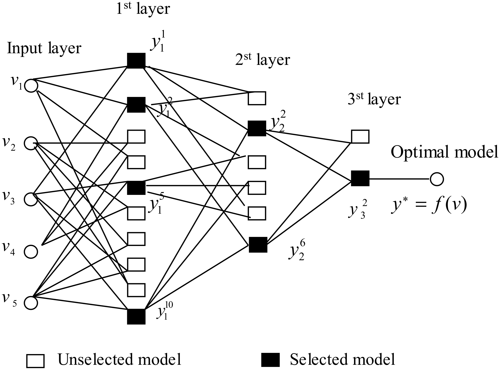
2.1. GMDH Network
2.2. Basic Modeling Idea
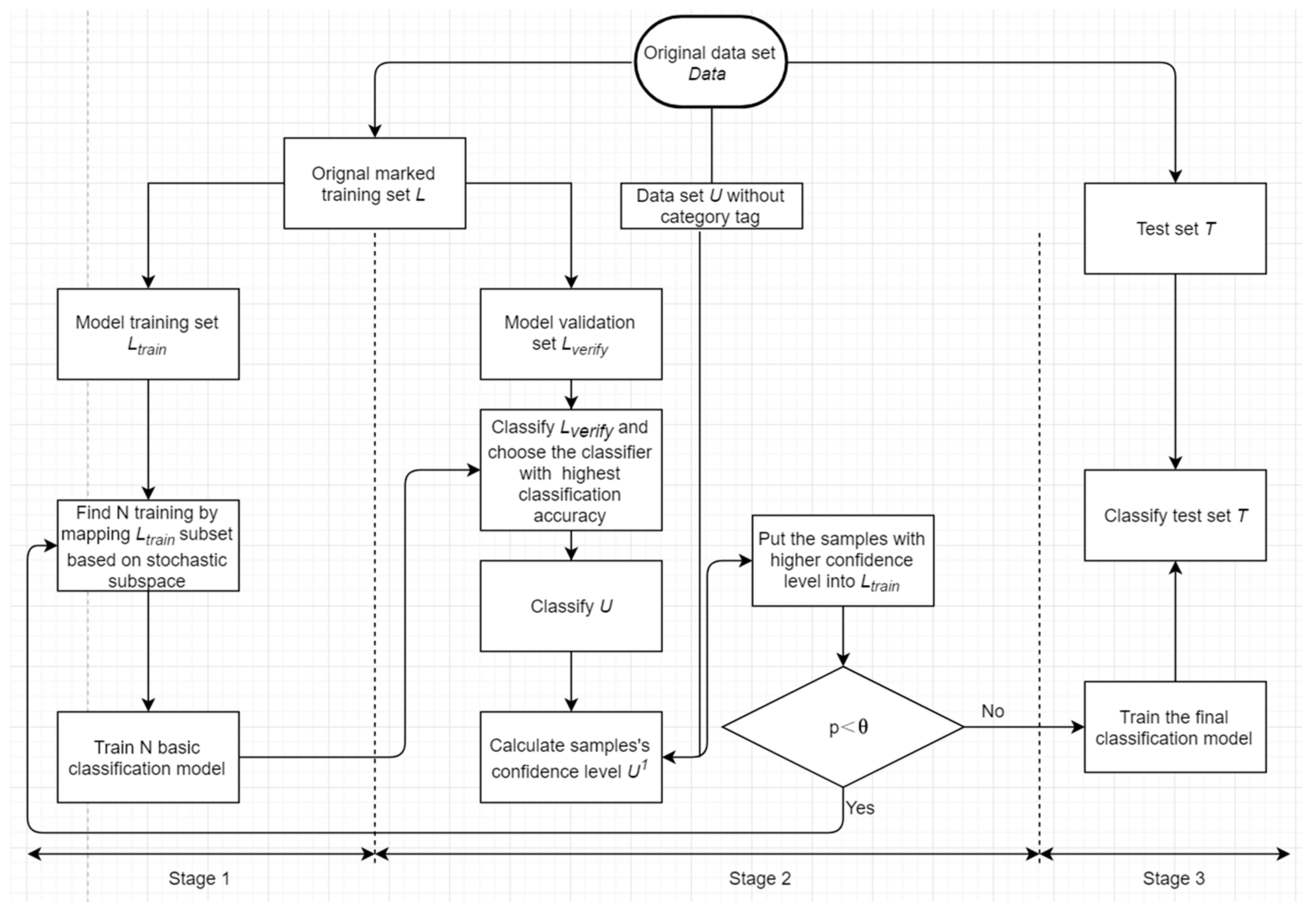
2.3. Detailed Modeling Steps
2.4. Establishing the GMDH External Criteria
3. Data Description
- -
- -
- Weather variables: There are six weather variables: the maximum temperature, minimum temperature, maximum temperature variable rate, minimum temperature variable rate, wind speed, and weather type. As the electricity load is susceptible to changes in weather variables, it is necessary to understand electricity load volatility under various weather conditions within different timescales [49]. Weather variables have been seen as the main parameters controlling energy demand [50,51].
- -
- Load series: There are eleven kinds of load series, namely the peak load, off-peak load, daily consumption, cumulative consumption, off-peak consumption, load rate, actual peak load, previous day’s electricity consumption, daily consumption in the same period of the previous week, daily consumption in the same period in the previous month, and daily consumption in the same period of the previous year.
- -
- : is defined as the peak load and as the number of categories, such that . The specification for is as follows:where and denote the maximal peak load and the minimal peak load, respectively, and is defined as the step length that is set based on the power of generators.
4. Empirical Analysis
4.1. Experimental Setting
4.2. Model Evaluation Criteria
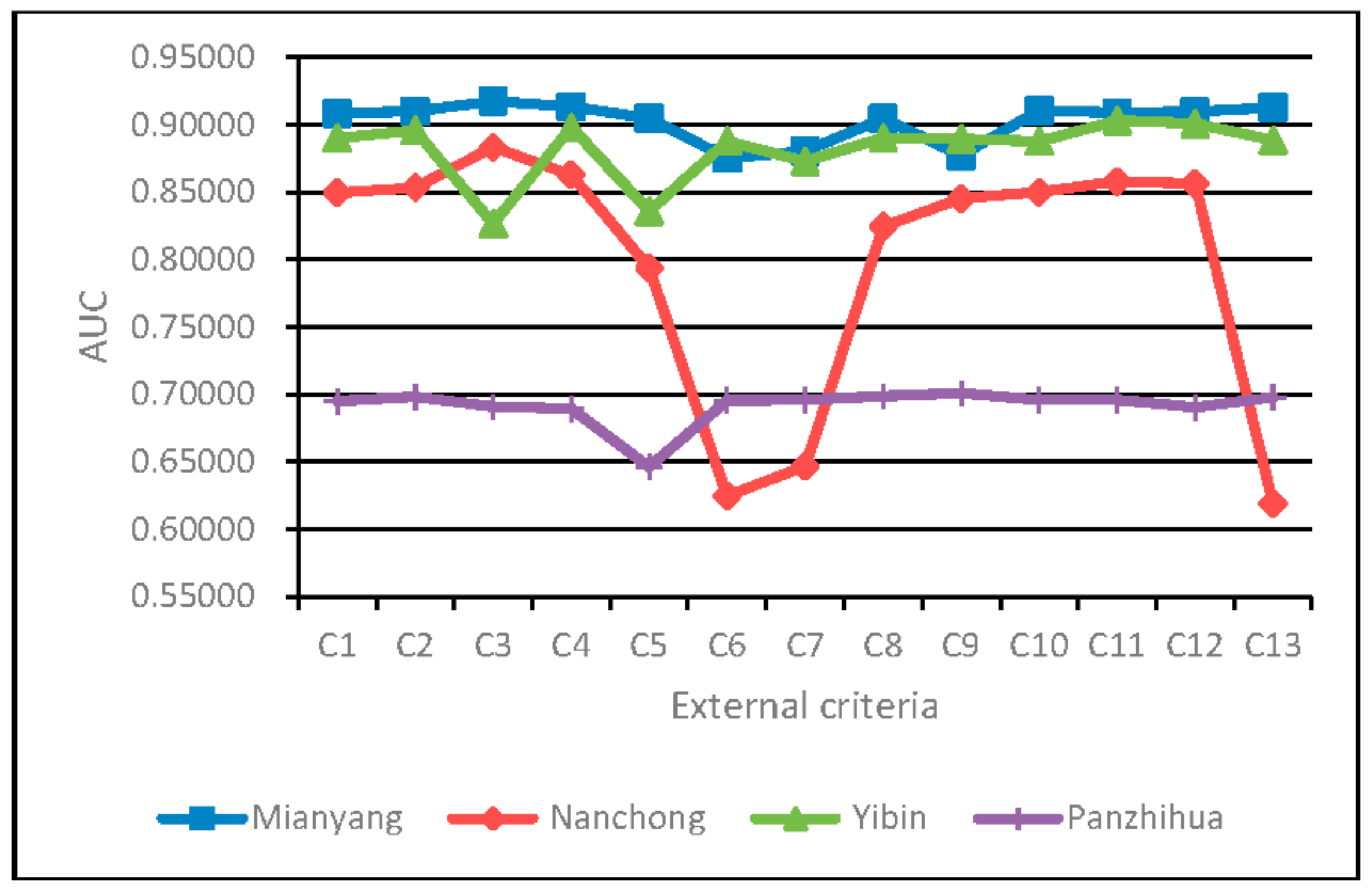
4.3. Analysis of the Impacts of the GMDH External Criteria on Classification Performance of the SSFS-GMDH Model
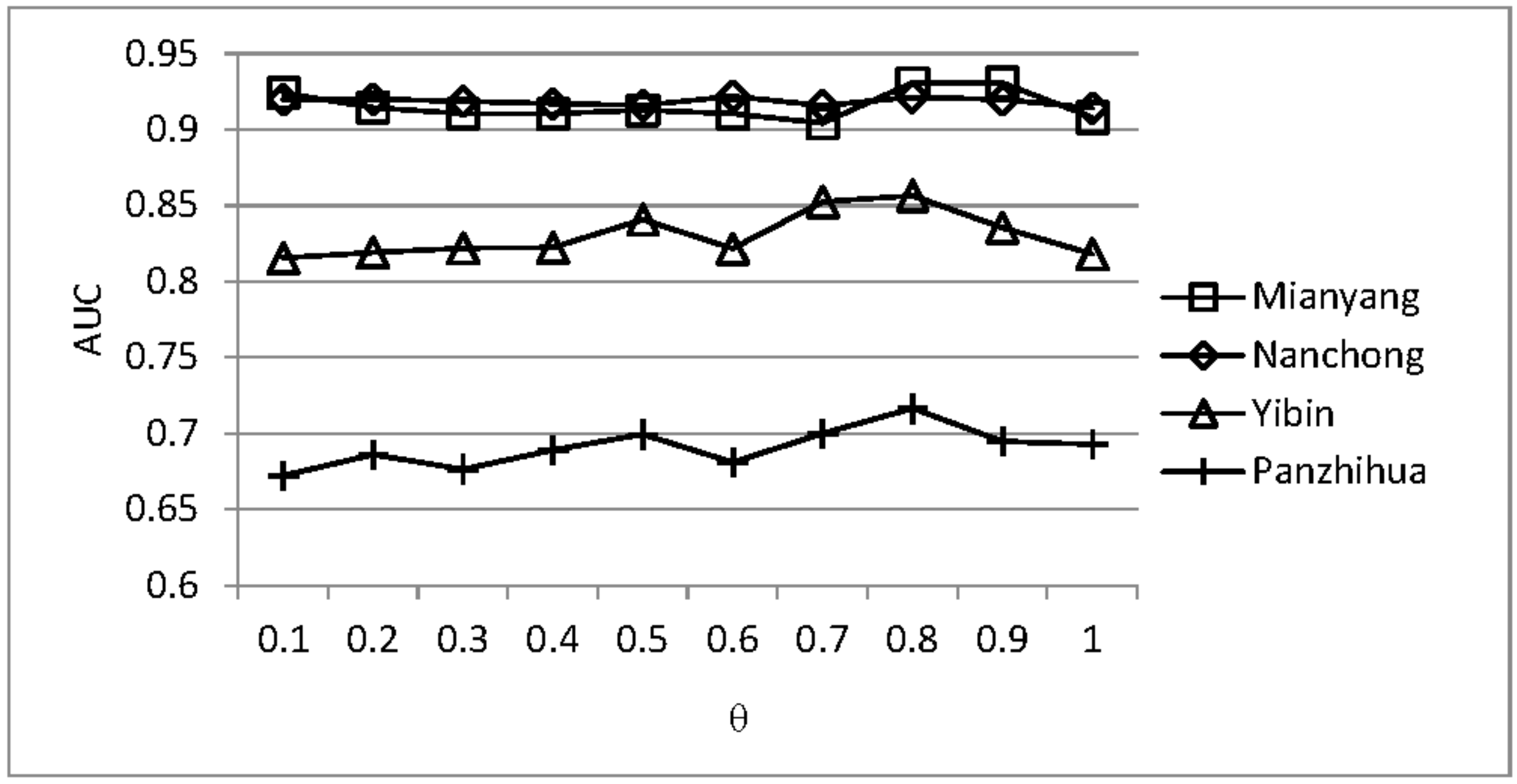
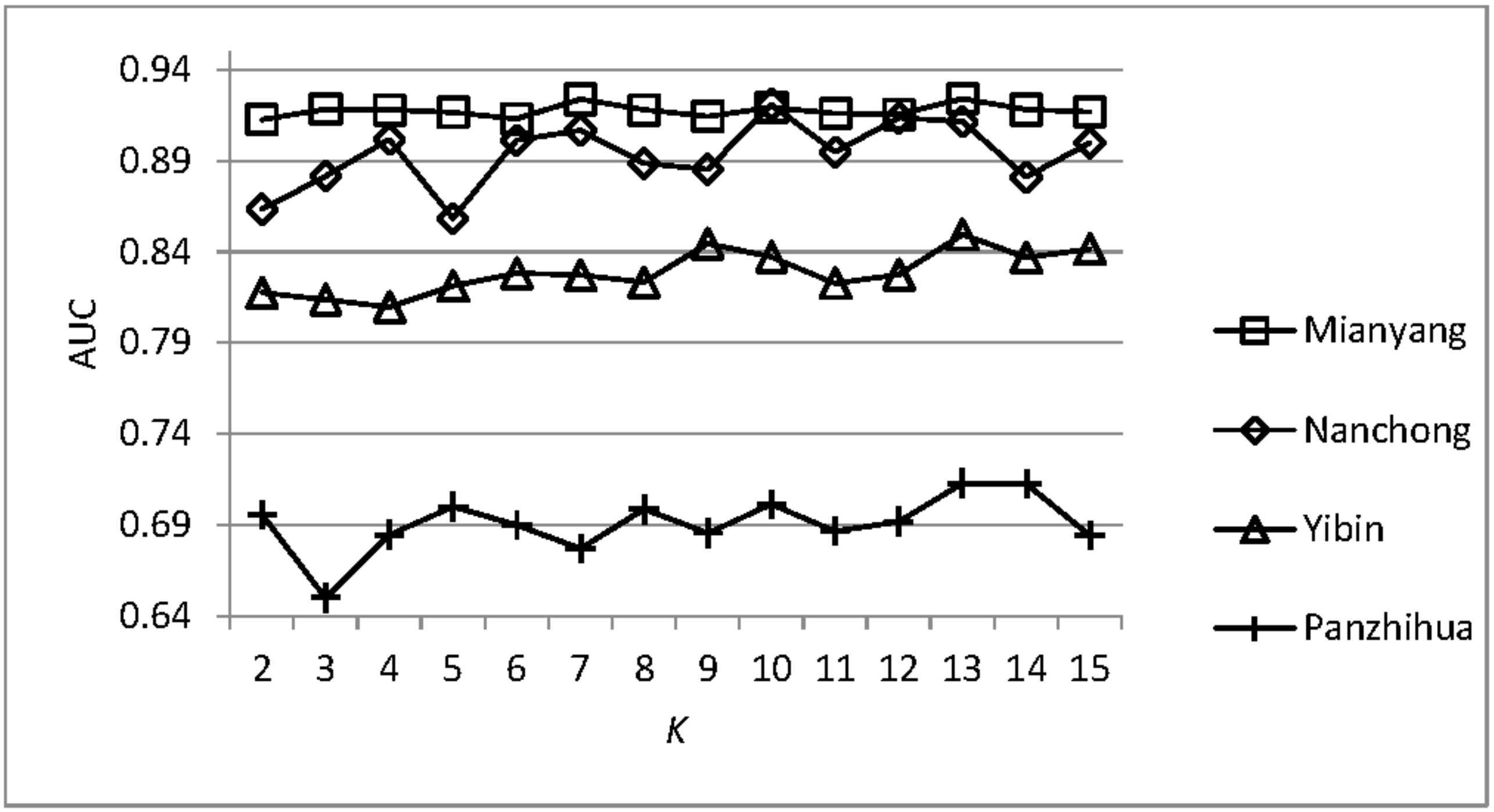
4.4. Analysis of the Parameter Sensitivity
4.5. Comparisons with Other Models
5. Conclusions
Author Contributions
Conflicts of Interest
References
- Chen, B.-J.; Chang, M.-W. Load forecasting using support vector machines: A study on eunite competition 2001. IEEE Trans. Power Syst. 2004, 19, 1821–1830. [Google Scholar] [CrossRef]
- Fan, G.-F.; Peng, L.-L.; Hong, W.-C.; Sun, F. Electric load forecasting by the svr model with differential empirical mode decomposition and auto regression. Neurocomputing 2016, 173, 958–970. [Google Scholar] [CrossRef]
- Andersen, F.M.; Larsen, H.V.; Gaardestrup, R.B. Long term forecasting of hourly electricity consumption in local areas in denmark. Appl. Energy 2013, 110, 147–162. [Google Scholar] [CrossRef]
- De Felice, M.; Alessandri, A.; Catalano, F. Seasonal climate forecasts for medium-term electricity demand forecasting. Appl. Energy 2015, 137, 435–444. [Google Scholar] [CrossRef]
- Taylor, J.W.; McSharry, P.E. Short-term load forecasting methods: An evaluation based on european data. IEEE Trans. Power Syst. 2007, 22, 2213–2219. [Google Scholar] [CrossRef]
- Hong, T. Short Term Electric Load Forecasting; North Carolina State University: Raleigh, NC, USA, 2010; pp. 3–6. [Google Scholar]
- Liu, J.-P.; Li, C.-L. The short-term power load forecasting based on sperm whale algorithm and wavelet least square support vector machine with DWT-IR for feature selection. Sustainability 2017, 9, 1188. [Google Scholar] [CrossRef]
- Taylor, J.W. An evaluation of methods for very short-term load forecasting using minute-by-minute british data. Int. J. Forecast. 2008, 24, 645–658. [Google Scholar] [CrossRef]
- Hong, T.; Fan, S. Probabilistic electric load forecasting: A tutorial review. Int. J. Forecast. 2016, 32, 914–938. [Google Scholar] [CrossRef]
- Hippert, H.S.; Pedreira, C.E.; Souza, R.C. Neural networks for short-term load forecasting: A review and evaluation. IEEE Trans. Power Syst. 2001, 16, 44–55. [Google Scholar] [CrossRef]
- Hong, T.; Gui, M.; Baran, M.E.; Willis, H.L. Modeling and forecasting hourly electric load by multiple linear regression with interactions. In Proceedings of the Power and Energy Society General Meeting, Providence, RI, USA, 25–29 July 2010; pp. 1–8. [Google Scholar]
- Wang, Y.; Xia, Q.; Kang, C. Secondary forecasting based on deviation analysis for short-term load forecasting. IEEE Trans. Power Syst. 2011, 26, 500–507. [Google Scholar] [CrossRef]
- Ceperic, E.; Ceperic, V.; Baric, A. A strategy for short-term load forecasting by support vector regression machines. IEEE Trans. Power Syst. 2013, 28, 4356–4364. [Google Scholar] [CrossRef]
- Paparoditis, E.; Sapatinas, T. Short-term load forecasting: The similar shape functional time-series predictor. IEEE Trans. Power Syst. 2013, 28, 3818–3825. [Google Scholar] [CrossRef]
- Chitsaz, H.; Shaker, H.; Zareipour, H.; Wood, D.; Amjady, N. Short-term electricity load forecasting of buildings in microgrids. Energy Build. 2015, 99, 50–60. [Google Scholar] [CrossRef]
- Ju, F.-Y.; Hong, W.-C. Application of seasonal svr with chaotic gravitational search algorithm in electricity forecasting. Appl. Math. Model. 2013, 37, 9643–9651. [Google Scholar] [CrossRef]
- Desha, C.J.K.; Smith, M.; Hargroves, K.J.; Stasinopoulos, P.; Stephens, R. Energy Transformed: Sustainable Energy Solutions for Climate Change Mitigation; The Natural Edge Project, CSIRO, and Griffith University: Brisbane, Australia, 2007. [Google Scholar]
- Staff, G.B. Unlocking Energy Efficiency in the U.S. Economy; Mckinsey & Company: Chicago, IL, USA, 2009. [Google Scholar]
- Bessec, M.; Fouquau, J. Short-run electricity load forecasting with combinations of stationary wavelet transforms. Eur. J. Oper. Res. 2018, 264, 149–164. [Google Scholar] [CrossRef]
- Feng, Y.; Ryan, S.M. Day-ahead hourly electricity load modeling by functional regression. Appl. Energy 2016, 170, 455–465. [Google Scholar] [CrossRef]
- Tong, C.; Li, J.; Lang, C.; Kong, F.; Niu, J.; Rodrigues, J.J.P.C. An efficient deep model for day-ahead electricity load forecasting with stacked denoising auto-encoders. J. Parallel Distrib. Comput. 2017, in press. [Google Scholar] [CrossRef]
- Amjady, N. Short-term hourly load forecasting using time-series modeling with peak load estimation capability. IEEE Trans. Power Syst. 2001, 16, 498–505. [Google Scholar] [CrossRef]
- Okoboi, G.; Mawejje, J. Electricity peak demand in uganda: Insights and foresight. Energy Sustain. Soc. 2016, 6, 29. [Google Scholar] [CrossRef]
- Alani, A.Y.; Osunmakinde, I.O. Short-term multiple forecasting of electric energy loads for sustainable demand planning in smart grids for smart homes. Sustainability 2017, 9, 1972. [Google Scholar] [CrossRef]
- Kim, Y.-J. Comparison between inverse model and chaos time series inverse model for long-term prediction. Sustainability 2017, 9, 982. [Google Scholar] [CrossRef]
- Zhang, Z.; Song, Y.; Liu, F.; Liu, J. Daily average wind power interval forecasts based on an optimal adaptive-network-based fuzzy inference system and singular spectrum analysis. Sustainability 2016, 8, 125. [Google Scholar] [CrossRef]
- Hu, Y.-C. Nonadditive grey prediction using functional-link net for energy demand forecasting. Sustainability 2017, 9, 1166. [Google Scholar] [CrossRef]
- Weron, R. Electricity price forecasting: A review of the state-of-the-art with a look into the future. Int. J. Forecast. 2014, 30, 1030–1081. [Google Scholar] [CrossRef]
- Andrade, J.R.; Filipe, J.; Reis, M.; Bessa, R.J. Probabilistic price forecasting for day-ahead and intraday markets: Beyond the statistical model. Sustainability 2017, 9, 1990. [Google Scholar] [CrossRef]
- Box, G.E.P.; Jenkins, G.M. Time Series Analysis: Forecasting and Control; John Wiley & Sons: Oakland, CA, USA, 1976; Volume 31, p. 303. [Google Scholar]
- Soares, L.J.; Medeiros, M.C. Modeling and forecasting short-term electricity load: A comparison of methods with an application to brazilian data. Int. J. Forecast. 2008, 24, 630–644. [Google Scholar] [CrossRef]
- Cincotti, S.; Gallo, G.; Ponta, L.; Raberto, M. Modeling and forecasting of electricity spot-prices: Computational intelligence vs. classical econometrics. AI Commun. 2014, 27, 301–314. [Google Scholar]
- Amjady, N.; Keynia, F. Day ahead price forecasting of electricity markets by a mixed data model and hybrid forecast method. Int. J. Electr. Power Energy Syst. 2008, 30, 533–546. [Google Scholar] [CrossRef]
- Mori, H.; Takahashi, A. Hybrid intelligent method of relevant vector machine and regression tree for probabilistic load forecasting. In Proceedings of the 2011 2nd IEEE PES International Conference and Exhibition on Innovative Smart Grid Technologies (ISGT Europe), Manchester, UK, 5–7 December 2011; pp. 1–8. [Google Scholar]
- Xiong, T.; Bao, Y.; Hu, Z. Interval forecasting of electricity demand: A novel bivariate emd-based support vector regression modeling framework. Int. J. Electr. Power Energy Syst. 2014, 63, 353–362. [Google Scholar] [CrossRef]
- Dag, O.; Yozgatligil, C. Gmdh: An R package for short term forecasting via gmdh-type neural network algorithms. R J. 2016, 8, 379–386. [Google Scholar]
- Chen, L.-G.; Chiang, H.-D.; Dong, N.; Liu, R.-P. Group-based chaos genetic algorithm and non-linear ensemble of neural networks for short-term load forecasting. IET Gener. Transm. Distrib. 2016, 10, 1440–1447. [Google Scholar] [CrossRef]
- Ratrout, N. Short-term traffic flow prediction using group method data handling (gmdh)-based abductive networks. Arab. J. Sci. Eng. 2014, 39, 631–646. [Google Scholar] [CrossRef]
- Kim, D.; Seo, S.-J.; Park, G.-T. Hybrid gmdh-type modeling for nonlinear systems: Synergism to intelligent identification. Adv. Eng. Softw. 2009, 40, 1087–1094. [Google Scholar] [CrossRef]
- Ivakhnenko, A.G.; Ivakhnenko, G.A. The review of problems solvable by algorithms of the group method of data handling (gmdh). Pattern Recognit. Image Anal. 1995, 5, 527–535. [Google Scholar]
- Ivakhnenko, A.G.; Ivakhnenko, G.A. Problems of further development of the group method of data handling algorithms. Pattern Recognit. Image Anal. 2000, 10, 187–194. [Google Scholar]
- Shaghaghi, S.; Bonakdari, H.; Gholami, A.; Ebtehaj, I.; Zeinolabedini, M. Comparative analysis of gmdh neural network based on genetic algorithm and particle swarm optimization in stable channel design. Appl. Math. Comput. 2017, 313, 271–286. [Google Scholar] [CrossRef]
- Xiao, J.; He, C.; Jiang, X.; Liu, D. A dynamic classifier ensemble selection approach for noise data. Inf. Sci. 2010, 180, 3402–3421. [Google Scholar] [CrossRef]
- Xiao, J.; He, C.; Jiang, X. Structure identification of bayesian classifiers based on gmdh. Knowl.-Based Syst. 2009, 22, 461–470. [Google Scholar] [CrossRef]
- McAfee, A.; Brynjolfsson, E.; Davenport, T.H. Big data: The management revolution. Harv. Bus. Rev. 2012, 90, 60–68. [Google Scholar] [PubMed]
- Xiao, J.; Cao, H.; Jiang, X.; Gu, X.; Xie, L. Gmdh-based semi-supervised feature selection for customer classification. Knowl.-Based Syst. 2017, 132, 236–248. [Google Scholar] [CrossRef]
- Takeda, H.; Tamura, Y.; Sato, S. Using the ensemble kalman filter for electricity load forecasting and analysis. Energy 2016, 104, 184–198. [Google Scholar] [CrossRef]
- Bauer, M.; Scartezzini, J.L. A simplified correlation method accounting for heating and cooling loads in energy-efficient buildings. Energy Build. 1998, 27, 147–154. [Google Scholar] [CrossRef]
- Wang, Y.; Bielicki, J.M. Acclimation and the response of hourly electricity loads to meteorological variables. Energy 2018, 142, 473–485. [Google Scholar] [CrossRef]
- Sailor, D.J.; Muñoz, J.R. Sensitivity of electricity and natural gas consumption to climate in the U.S.A.—Methodology and results for eight states. Energy 1997, 22, 987–998. [Google Scholar] [CrossRef]
- Valor, E.; Meneu, V.; Caselles, V. Daily air temperature and electricity load in spain. J. Appl. Meteorol. 2001, 40, 1413–1421. [Google Scholar] [CrossRef]
- Ren, J.; Qiu, Z.; Fan, W.; Cheng, H.; Philip, S.Y. Forward semi-supervised feature selection. In Proceedings of the Pacific-Asia Conference on Knowledge Discovery and Data Mining, Osaka, Japan, 20–23 May 2008; Springer: Berlin/Heidelberg, Germany, 2008; pp. 970–976. [Google Scholar]
- Lee, K.; Park, I.; Yoon, B. An approach for r&d partner selection in alliances between large companies, and small and medium enterprises (smes): Application of bayesian network and patent analysis. Sustainability 2016, 8, 117. [Google Scholar]
- Tso, G.K.; Yau, K.K. Predicting electricity energy consumption: A comparison of regression analysis, decision tree and neural networks. Energy 2007, 32, 1761–1768. [Google Scholar] [CrossRef]
- Huang, N.; Zhang, S.; Cai, G.; Xu, D. Power quality disturbances recognition based on a multiresolution generalized s-transform and a pso-improved decision tree. Energies 2015, 8, 549–572. [Google Scholar] [CrossRef]
- Webb, G.I.; Ting, K.M. On the application of roc analysis to predict classification performance under varying class distributions. Mach. Learn. 2005, 58, 25–32. [Google Scholar] [CrossRef]


| Symbols | Interpretation |
|---|---|
| L | original labeled training set |
| T | labeled testing set |
| U | unlabeled dataset |
| chosen unlabeled sample | |
| marked unlabeled sample | |
| training set | |
| validation set | |
| N | the number of basic classification models |
| feature set | |
| the number of neighboring samples | |
| , | the proportion of samples chosen to be added into training set |
| the confidence level |
| Categories of Indicators | Sub-Indicators |
|---|---|
| Weather variables | W1: Maximum temperature (°C) |
| W2: Minimum temperature (°C) | |
| W3: Maximum temperature variable rate | |
| W4: Minimum temperature variable rate | |
| W5: Wind speed (m/s) | |
| W6: Weather type | |
| Calendar variables | C1: Calendar, such as holidays, weekdays and weekends. |
| Load series | L1: Peak load |
| L2: Off-peak load | |
| L3: Daily consumption | |
| L4: Cumulative consumption | |
| L5: Off-peak consumption | |
| L6: Load rate | |
| L7: Actual peak load | |
| L8: Previous day’s electricity consumption | |
| L9: Daily consumption in the same period of the previous week | |
| L10: Daily consumption in the same period in the previous month | |
| L11: Daily consumption in the same period of the previous year |
| Symbols | Parameters Setting |
|---|---|
| L | 30% |
| T | 40% |
| U | 30% |
| N | 3 |
| , |
| Class Predicted to Be Positive | Class Predicted to Be Negative | |
|---|---|---|
| Positive Class | TP | FN |
| Negative Class | FP | TN |
| Mianyang, China | |||||||||||||
|---|---|---|---|---|---|---|---|---|---|---|---|---|---|
| C1 | C2 | C3 | C4 | C5 | C6 | C7 | C8 | C9 | C10 | C11 | C12 | C13 | |
| C1 | 0.477 | 0.000 | 0.024 | 0.117 | 0.000 | 0.000 | 0.104 | 0.000 | 0.300 | 0.777 | 0.582 | 0.053 | |
| C2 | 0.001 | 0.122 | 0.023 | 0.000 | 0.000 | 0.020 | 0.000 | 0.745 | 0.669 | 0.872 | 0.222 | ||
| C3 | 0.073 | 0.000 | 0.000 | 0.000 | 0.000 | 0.000 | 0.003 | 0.000 | 0.000 | 0.034 | |||
| C4 | 0.000 | 0.000 | 0.000 | 0.000 | 0.000 | 0.222 | 0.049 | 0.088 | 0.746 | ||||
| C5 | 0.000 | 0.000 | 0.953 | 0.000 | 0.009 | 0.065 | 0.034 | 0.000 | |||||
| C6 | 0.023 | 0.000 | 0.366 | 0.000 | 0.000 | 0.000 | 0.000 | ||||||
| C7 | 0.000 | 0.169 | 0.000 | 0.000 | 0.000 | 0.000 | |||||||
| C8 | 0.000 | 0.008 | 0.056 | 0.030 | 0.000 | ||||||||
| C9 | 0.000 | 0.000 | 0.000 | 0.000 | |||||||||
| C10 | 0.452 | 0.627 | 0.370 | ||||||||||
| C11 | 0.790 | 0.099 | |||||||||||
| C12 | 0.167 | ||||||||||||
| C13 | |||||||||||||
| Nanchong, China | |||||||||||||
| C1 | C2 | C3 | C4 | C5 | C6 | C7 | C8 | C9 | C10 | C11 | C12 | C13 | |
| C1 | 0.608 | 0.000 | 0.080 | 0.000 | 0.000 | 0.000 | 0.001 | 0.595 | 0.940 | 0.276 | 0.376 | 0.000 | |
| C2 | 0.000 | 0.216 | 0.000 | 0.000 | 0.000 | 0.000 | 0.296 | 0.661 | 0.564 | 0.710 | 0.000 | ||
| C3 | 0.009 | 0.000 | 0.000 | 0.000 | 0.000 | 0.000 | 0.000 | 0.001 | 0.000 | 0.000 | |||
| C4 | 0.000 | 0.000 | 0.000 | 0.000 | 0.023 | 0.094 | 0.508 | 0.386 | 0.000 | ||||
| C5 | 0.000 | 0.000 | 0.000 | 0.000 | 0.000 | 0.000 | 0.000 | 0.000 | |||||
| C6 | 0.005 | 0.000 | 0.000 | 0.000 | 0.000 | 0.000 | 0.476 | ||||||
| C7 | 0.000 | 0.000 | 0.000 | 0.000 | 0.000 | 0.000 | |||||||
| C8 | 0.007 | 0.001 | 0.000 | 0.000 | 0.000 | ||||||||
| C9 | 0.544 | 0.105 | 0.157 | 0.000 | |||||||||
| C10 | 0.310 | 0.418 | 0.000 | ||||||||||
| C11 | 0.837 | 0.000 | |||||||||||
| C12 | 0.000 | ||||||||||||
| C13 | |||||||||||||
| Panzhihua, China | |||||||||||||
| C1 | C2 | C3 | C4 | C5 | C6 | C7 | C8 | C9 | C10 | C11 | C12 | C13 | |
| C1 | 0.235 | 0.000 | 0.087 | 0.000 | 0.636 | 0.000 | 0.995 | 0.904 | 0.599 | 0.006 | 0.025 | 0.745 | |
| C2 | 0.000 | 0.602 | 0.000 | 0.097 | 0.000 | 0.238 | 0.191 | 0.087 | 0.118 | 0.288 | 0.131 | ||
| C3 | 0.000 | 0.047 | 0.000 | 0.000 | 0.000 | 0.000 | 0.000 | 0.000 | 0.000 | 0.000 | |||
| C4 | 0.000 | 0.029 | 0.000 | 0.089 | 0.067 | 0.025 | 0.297 | 0.589 | 0.042 | ||||
| C5 | 0.000 | 0.000 | 0.000 | 0.000 | 0.000 | 0.000 | 0.000 | 0.000 | |||||
| C6 | 0.002 | 0.631 | 0.724 | 0.958 | 0.001 | 0.007 | 0.882 | ||||||
| C7 | 0.000 | 0.000 | 0.002 | 0.000 | 0.000 | 0.001 | |||||||
| C8 | 0.899 | 0.595 | 0.006 | 0.025 | 0.740 | ||||||||
| C9 | 0.685 | 0.004 | 0.018 | 0.838 | |||||||||
| C10 | 0.001 | 0.006 | 0.841 | ||||||||||
| C11 | 0.616 | 0.002 | |||||||||||
| C12 | 0.010 | ||||||||||||
| C13 | |||||||||||||
| Yibin, China | |||||||||||||
| C1 | C2 | C3 | C4 | C5 | C6 | C7 | C8 | C9 | C10 | C11 | C12 | C13 | |
| C1 | 0.447 | 0.359 | 0.230 | 0.000 | 0.878 | 0.822 | 0.407 | 0.182 | 0.820 | 0.835 | 0.316 | 0.508 | |
| C2 | 0.093 | 0.050 | 0.000 | 0.543 | 0.592 | 0.946 | 0.567 | 0.593 | 0.580 | 0.078 | 0.921 | ||
| C3 | 0.777 | 0.000 | 0.284 | 0.253 | 0.081 | 0.024 | 0.253 | 0.261 | 0.932 | 0.114 | |||
| C4 | 0.000 | 0.176 | 0.154 | 0.043 | 0.011 | 0.153 | 0.159 | 0.843 | 0.063 | ||||
| C5 | 0.000 | 0.000 | 0.000 | 0.000 | 0.000 | 0.000 | 0.000 | 0.000 | |||||
| C6 | 0.943 | 0.500 | 0.238 | 0.941 | 0.957 | 0.248 | 0.611 | ||||||
| C7 | 0.546 | 0.267 | 0.999 | 0.986 | 0.220 | 0.662 | |||||||
| C8 | 0.613 | 0.548 | 0.535 | 0.067 | 0.868 | ||||||||
| C9 | 0.268 | 0.260 | 0.020 | 0.501 | |||||||||
| C10 | 0.985 | 0.219 | 0.664 | ||||||||||
| C11 | 0.226 | 0.650 | |||||||||||
| C12 | 0.096 | ||||||||||||
| C13 | |||||||||||||
| Classification Model | Mianyang | Nanchong | Yibin | Panzhihua |
|---|---|---|---|---|
| SSFS-GMDH3 | 0.9452 | 0.9160 | 0.8640 | 0.7188 |
| SSFS-GMDH11 | 0.9381 | 0.8621 | 0.9077 | 0.7491 |
| FW-SemiFS | 0.9308 | 0.8520 | 0.8419 | 0.6188 |
| GMDH-U | 0.9218 | 0.8548 | 0.8611 | 0.6476 |
© 2018 by the authors. Licensee MDPI, Basel, Switzerland. This article is an open access article distributed under the terms and conditions of the Creative Commons Attribution (CC BY) license (http://creativecommons.org/licenses/by/4.0/).
Share and Cite
Yang, L.; Yang, H.; Liu, H. GMDH-Based Semi-Supervised Feature Selection for Electricity Load Classification Forecasting. Sustainability 2018, 10, 217. https://doi.org/10.3390/su10010217
Yang L, Yang H, Liu H. GMDH-Based Semi-Supervised Feature Selection for Electricity Load Classification Forecasting. Sustainability. 2018; 10(1):217. https://doi.org/10.3390/su10010217
Chicago/Turabian StyleYang, Lintao, Honggeng Yang, and Haitao Liu. 2018. "GMDH-Based Semi-Supervised Feature Selection for Electricity Load Classification Forecasting" Sustainability 10, no. 1: 217. https://doi.org/10.3390/su10010217
APA StyleYang, L., Yang, H., & Liu, H. (2018). GMDH-Based Semi-Supervised Feature Selection for Electricity Load Classification Forecasting. Sustainability, 10(1), 217. https://doi.org/10.3390/su10010217