Static and Dynamic Pricing Strategies in a Closed-Loop Supply Chain with Reference Quality Effects

Abstract

Remanufacturing of returned products has been increasingly recognized in industries as an effective approach to face environmental responsibility, government regulations, and increased awareness of consumers. In this paper, we address a closed-loop supply chain (CLSC) in which the manufacturer produces the brand-new products, as well as the remanufactured goods while the retailer sells these products to customers. We consider several different scenarios: the manufacturer and the retailer adopt a steady-state price or a dynamic price with reference quality effects in a centralized case; either, neither or both the manufacturer and the retailer price dynamically with reference quality effects, respectively, in a decentralized model. We solve the problem with the retailer recycling the sold copies and deduce the optimal pricing strategies while the manufacturer in charge of recovering the used items in such a CLSC. The result shows that dynamic pricing strategies are much more profitable for the supply chain and its members when compared with pricing statically; the dynamic pricing strategies with time-varying quality characterized by reference quality are more suited to a long-term and cooperative closed-loop supply chain. Moreover, the optimal recycling fraction relies on the recovery cost coefficient and proves to be uniform despite adopting a dynamic price and quality in all distinct cases.

1. Introduction

As the global economy prospered and advanced technology widely used, so many diversified products move towards consumers like an unstoppable wave that the life of products becomes shorter and shorter, the speed of renewing goods gets faster and faster, which make the total amount and the growth ratio of the waste rise. Approximately 1.3 billion tons of solid waste was generated in cities worldwide in 2017. It is estimated that by 2025, the annual amount of solid waste will be about two times greater than the amount in 2017 [1,2]. Meanwhile, the circular economy, replacing the “take, make, consume, and dispose” patterns with closed-loops of material flows by combining a number of different processes including maintenance, repair, reusing, refurbishing, remanufacturing, and recycling, has created much more concern in the academic world and in practice [2,3]. As such, remanufacturing, as a crucial component of the circular economy, has been regarded as a potential method to deal with economic, social, and environmental problems [4,5,6,7]. Many manufacturers have implemented remanufacturing policies, consisting of taking back and processing returned products partly to comply with environmental legislation and partly due to the potential profit generated by sustainable production [8]. The closed-loop supply chain, regarded as one of most effective approaches to deal with the waste for economically and environmentally, has become a common sense approach to recycling and reusing end-of-life products both in industry and academia [9,10].

The recycling model or reverse channel is one of key influencing factors that determines the efficiency and effectiveness of recycling in a closed-loop supply chain (CLSC). There are three typical recycling channels in extant researches and practice: the manufacturer collecting the sold products directly from consumers, the manufacturer contracting the collection of used items to the retailer, and the manufacturer contracting the collection of used items to a third party [11]. The recycling model, as well as the recovery fraction and recycling costs, which are factors of the recycling policy, play an important role in influencing the profits of the remanufacturing supply chain and its members [12,13,14]. To achieve an optimal recycling policy, this paper constructs a closed-loop supply chain with the retailer collecting the used products and tries to compare it with the case where the manufacture collects the sold items directly.

Quality, as an influential medium to affect product price, sales, and other market conditions, is presented. The quality of the original product can directly determine the difficulty of the product recovery, and even the recycling policy. If the used product is poor in quality, the entire remanufacturing process might not be economically profitable and therefore, the whole remanufacturing supply chain system taking up pure production with no recycling could be the optimal solution [15]. On the other hand, consumers have a strong willingness to exchange the returned items in the recycling system for a higher transaction price if the sold goods have a better quality. However, the product quality is often inconsistent with the real quality perceived by consumers [16,17]. The real quality customers expect is referred to as “reference quality”. If the reference quality of the new items exceeds that of the customers’ previous expectation, consumers’ impression and loyalty to the product will be greatly improved, which can lead to greater sales and vice versa. Thus, the relationship between the quality system (including product quality and reference quality) and the strategy system (including pricing and recycling policy) is a meaningful topic that is worthy of deep exploration.

An appropriate pricing strategy will definitely be instrumental in increasing profits, leading to a better market share for the firm. The industry pays much more attention to pricing strategy, which is deemed to be a predominant marketing tool, regardless of pricing statically or dynamically. Overall, pricing dynamically, viz. making pricing decisions after the demand and the other factors are disclosed, is seen as a superior pricing policy for stakeholders to characterize a dynamic and uncertain market environment [18]. Dynamic pricing strategy, as an influential method to provide increased benefits, has wide international recognition among firms experiencing fierce competition that is caused by the rapid development of e-commerce and product updates. The advantage of pricing dynamically exists for the traditional supply chain [19,20]; whether dynamic pricing is applicable to the closed-loop supply chain consisting of new products, as well as remanufactured goods, as well as what influences dynamic pricing strategies have on a closed-loop supply chain, is unknown.

Motivated by the above facts, we address a closed-loop supply chain where the manufacturer and the retailer adopt dynamic pricing strategies with reference quality effects. The manufacturer has alternative channels to meet the customers’ demand: one is producing brand-new goods from pure raw materials and the other is transforming used products into as-good-as new ones. We will address the following questions: (1) What are the optimum quality, reference quality, wholesale price, and retail price for a closed-loop supply chain and its members for both centralized and decentralized cases? (2) What is the interactive influence between the dynamic quality, the reference quality, and pricing in different cases? (3) Which kind of pricing strategies are best for the retailer, the manufacturer, and the total supply chain, respectively? (4) Do the dynamic pricing strategies really stimulate the collection quantity and proportion of available used items in a closed-loop supply chain and what is the best recovery policy for the system in dynamic pricing strategies?

For the sake of comparing the effectiveness of the various distinct pricing strategies with dynamic quality characterized by reference quality, we attempt to solve the model in several scenarios: (1) The whole supply chain adopts static and dynamic pricing strategies in a centralized scenario respectively; and, (2) In a decentralized case, either, neither or both the manufacturer and the retailer price dynamically, respectively.

The remainder of this paper is organized as follows. A literature review is represented in Section 2. In Section 3, the model setting is formulated, and the notation is defined. The analytic solution is presented by solving the Stackelberg game between the manufacturer and the retailer in both the centralized and decentralized cases in Section 4 and Section 5, respectively. Section 6 gives numerical examples and assesses the sensitivity of some key parameters to demonstrate the feasibility of the main results. Eventually, we conclude the paper with discussions and further research directions in Section 7.

2. Literature Review

The main purpose of our work is to investigate different pricing strategies in the presence of reference quality in a closed-loop supply chain. Hence, literature referenced in this paper are formed from several topics: closed-loop supply chain, pricing dynamically or statically, and the reference quality effects.

2.1. Closed-Loop Supply Chain

As for the CLSC, the quality of the brand-new and remanufactured product plays a significant role in the remanufacturing process. Atasu and Souza [5] proposed three typical product recovery policies and analyzed the impacts that they had on quality decisions. The results suggested that the way of recycling vigorously affected the quality choice of the closed-loop supply chain system. Product recovery form (product recycling reuses the components or product recycling is costly) generally promoted the quality decision of the firm, while the form (product recycling remains profitable without using the material or components) inversely increased the product quality choice. Maiti and Giri [15] considered a closed-loop supply chain in which the manufacturer provided a product with a decent quality available to consumers in the context of a third party collecting the used items. The best decisions were acquired for such a closed-loop supply chain with different cases. It was found that the centralized policy was always optimal, and among the four decentralized cases, the retailer-led one was much more profitable. Ahmed et al. [21] assumed that the recovery fraction of returned items was a variable controlled by two related decision coefficients, which were the buying price for returned goods corresponding to an acceptable quality level.

However, the demand is not only sensitive to a measurable quality of product, but also is affected by the consumer’s perceived quality [22]. Hazen et al. [23] studied the perceptual quality of remanufactured goods from construct and measure development perspectives and found that perceived quality of remanufacturing products was sensitive to performance, features, lifetime, and service level. Wang and Hazen [6] revealed that purchase intention of remanufactured products was positively affected by perceived value, which was influenced by quality knowledge, cost knowledge, and green knowledge, respectively, via structural equation modeling.

Since dynamics is a prominent problem in the operation of modern enterprises, the decision variables have dynamic characteristics, particularly for a closed-loop supply chain in the market environment. Xu and Zhu [24] designed a non-linear dynamic pricing model to research the demand and the collection rate of used items affected by price and reference price, and pointed out that in the long term, the price of the ultimate product and the recycling price of used items was fixed to a certain value ignoring reference to the initial price of new goods and the recycling price of the used items. Huang and Nie [25] considered a closed-loop supply chain with a dynamic used-product collection fraction by building the differential equation about product return fraction. It was found that the recovery fraction and the collection effort were growing while the retail price and wholesale price were declining with time. Li et al. [26] proposed the concept of product reliability that relied on the quality and the time-utility value of the product and found that the pursuit of this strategy, especially the restructure and operation in a closed-loop supply chain, played a critical role in product quality.

Due to both the quality of the product and the reference quality perceived by the customer are sensitive to the profits of a supply chain and its members. In the market environment, quality has dynamic characteristics, as does the reference quality. Few researchers focus on the dynamic product quality and the reference quality for such a closed-loop supply chain in extant literatures. Furthermore, the decision variables are closely interrelated, for example, price is always a response to the quality of product. How does the dynamic quality affect the pricing strategies in a closed-loop supply chain? Consequently, we employed a dynamic pricing strategy with time-varying quality on the basis of reference quality effects in a closed-loop supply chain.

2.2. Dynamic Pricing Strategy

Being regarded as a superior pricing policy, many firms utilize time-varying pricing to gain more profits. Zhang et al. [27] compared the optimal strategies and profits for the supply chain with a time-varying reference price effect in distinct distribution channels. Shah et al. [28] constructed a Stackelberg game model with price markdown choice in a two-echelon supply chain. Wu et al. [19] employed a dynamic pricing and inventory strategy with reference effects being considered in both full retail price and price discount cases. Jia and Hu [29] investigated the time-varying ordering policy and dynamic price for deterioration items in a supply chain. Popescu and Wu [30] presented a dynamic pricing problem, in which demand was partly dependent on the firms’ previous pricing. Xu and Liu [31] discussed the reference price effect on the effectiveness across three decentralized reverse channels in a closed-loop supply chain. Zhang et al. [32] found that a two-part tariff contract was meaningful to coordinate the channel in a green supply chain within dynamic pricing in different cases. Ferrara et al. [33] constructed a dynamic pricing model of supply chain for corporate social responsibility.

The above researchers investigated a dynamic pricing strategy with a reference price or other decision variables, such as green innovation and corporate social responsibility. Moreover, product quality directly determines the price of the product and is always closely linked to the price. Gavious and Lowengart [16] considered a case in which the reference quality was a state variable to investigate the players’ pricing strategies. Zhang et al. [20] proposed dynamic and static pricing strategies in both centralized and decentralized scenarios with advertising taking reference quality effects into consideration. Kopalle and Winer [34] derived a case where the monopolist makes dynamic decisions considering price and expected product quality.

However, in spite of the obvious merits of time-varying pricing, some companies are still unwilling to modify pricing policies partly due to the potential adjustment costs and partly due to the consideration of customer psychology [35]. As a result, given that a comparison between dynamic and static pricing policies is vitally significant, which has already been seen in related researches, such as [20,35], it is clear that time-varying pricing policies apparently exceed steady-state pricing strategies with neglecting the adjustment cost, for the uniform pricing policy could be considered as a specific case of the time-varying one. By pricing statically, Ghosh and Shah [36] considered game theoretical models and presented how greening levels, pricing strategies, and profits were disrupted by channel structures. Krishnamurthi [37] investigated differences between the reference price, the purchase price, and ordering quantity, where consumers exhibited reference price. Liu et al. [38] focused on pricing strategies with three different supply chain network structures in two-stage Stackelberg game models. Karray and Sigue [39] gave a comparison about the pricing policy of different companies, in which one firm sold an independent product, while the other two sold complementary goods.

Additionally, the difference and the comparison between time-varying and steady-state pricing have rarely derived attention among researches. Cachon and Feldman [35] suggested that pricing statically provides more benefits compared with pricing dynamically when taking strategic consumers into consideration. Zhang et al. [20] compared the time-varying and steady-state pricing policies in both centralized and decentralized scenarios with advertising. Gayon and Dallery [40] combined pricing strategies with the optimum production decision, and then presented that time-varying pricing could be a better choice to increase benefits when production is partly constrained in a make-to-stock queue.

Few studies researched a dynamic pricing strategy in a closed-loop supply chain, particularly with pricing dynamically with reference quality effects. What is the best pricing strategy, pricing dynamically or pricing statically, if the dynamic quality and dynamic reference quality are considered in a closed-loop supply chain? Hence, this work tries to compare the dynamic pricing and uniform pricing taking dynamic product quality and reference quality into consideration in a closed-loop supply chain.

2.3. Reference Quality Effect

Product quality improvement has derived much more attention among academia. Singer et al. [17] constructed models for different strategic behavior considering product quality in a supplier-retailer partnership for disposable items. Li et al. [41] developed a grocery retail supply chain to avoid food spoilage waste and gained the optimal food retailer’s revenue via a pricing channel that is determined by dynamically identifying food shelf life. Chao et al. [42] investigated two contract mechanisms for product recycling cost sharing between a manufacturer and a supplier to stimulate quality improvement efforts. Xie et al. [43] researched a risk-averse supply chain combined with quality investment efforts and price decision under uncertain demand. Most of above studies think of quality as a uniform value, however, the firm always modifies the quality policy of product according to the market and consumers in a given period. The enterprise will make more (less) efforts to improve the product quality if customers are exposed to much more (less) qualified goods provided by its competitors. It signifies that relative quality among products does work when consumers make buying decisions, in other words, customers would set a benchmark of quality (perceived by previous product, observable information of the product and the product of its competitors) before they prepare to purchase this product.

Chenavaz [44] studied the dynamic quality strategy of a company whose customers utilized a reference quality when decision-making according to the principles of behavioral economics. The paper regards reference quality as an optimal control setting and determines solutions using Pontryagin’s maximum principle without considering the fact that price and quality are closely related. Accordingly, in accordance with firms’ practice in management, the relationship between the price and the dynamic quality strategy characterized by reference quality effects could not be neglected. Gavious and Lowengart [16] proposed an asymmetric and contractual agreement and investigated the impacts that the price and reference quality had on profits. Liu et al. [45] studied the reference quality effects combined with a revenue sharing contract in myopic and far-sighted scenarios. Kopalle and Winer [34] derived a case where the monopolists made dynamic decisions considering price and expected product quality. Zhang et al. [20] compared dynamic and static pricing strategies in a supply chain with advertising in the context of reference quality effect.

The aforementioned researches investigated the reference quality and dynamic quality in a traditional supply chain and few of them compared the pricing policies that are affected by dynamic quality and reference quality. However, in a closed-loop supply chain, the product system including brand-new products and remanufactured goods as well as the collection policy should be considered. Does this product system influence the optimal pricing strategy with dynamic quality characterized by reference quality? What is the best collection policy in such a pricing and quality strategy for a closed-loop supply chain? Hence, based on reference quality effect, we investigate dynamic quality and dynamic pricing strategies in a closed-loop supply chain.

In general, there is a large quantity of research literature on closed-loop supply chains, dynamic pricing, reference and dynamic quality. Nevertheless, there are few literatures researching the time-varying pricing strategies in the presence of dynamic quality characterized by reference quality effects in a closed-loop supply chain. We provide a specific comparison between the key literatures and our model shown in

Table 1. Our paper vs. the Literature.

Authors	rp	rq	dp	hf	CLSC	Focus
Gayon and Dallery [40]	√	×	√	×	×	Dynamic pricing, Markov decision, and make-to-stock queue
Liu et al. [45]	×	√	√	×	×	Reference quality, myopia, and revenue-sharing
Chenavaz [44]	×	√	×	√	×	Dynamic quality, reference quality, and behavioral economics
Kopalle and Winer [34]	√	√	√	√	×	Reference price and quality, and dynamic optimization
Gavious and Lowengart [16]	×	√	√	√	×	Optimal pricing, reference quality, and asymmetric
Zhang et al. [46]	√	×	√	√	×	Reference price, dynamic pricing, and distribution channel
Xu and Liu [31]	√	×	√	√	√	Reference price, reverse channel, and CLSC
Zhang et al. [20]	×	√	√	√	×	Dynamic, static, reference quality, and advertising
Our model	×	√	√	√	√	Dynamic, static, reference quality, and CLSC

Note: rp = reference price, rq = reference quality, dp = dynamic pricing, hf = hamilton function, CLSC = closed-loop supply chain.

. Above all, we develop a Stackelberg game between a manufacturer and a retailer in a closed-loop supply chain. The manufacturer is a leader who settles the quality level and the wholesale price, while the retailer is a follower who determines the retail price in the Stackelberg game.

Additionally, the purpose of this paper is to solve the problem using differential game with dynamic and static pricing strategies taking reference quality into consideration and explore the best recovery fraction for the closed-loop supply chain simultaneously.

3. Model and Notations

3.1. Notations

We define the variables with a set a concise and inerratic symbols. For ease of writing, we make some general rules for the symbols, such as R(t) means the reference quality, etc. (as shown in

Table 2. Notations and definitions.

Parameters	Meanings	Parameters	Meanings
$\alpha$	Basic market capacity	$k_2$	Recycling cost coefficient
$w(t)$	Wholesale price	${\gamma }_1$	Effect of product quality
$p(t)$	Retail price	${\gamma }_2$	Effect of the difference between q(t) and R(t)
$R(t)$	Reference quality	$\beta$	Price elasticity coefficient
$q(t)$	Quality	$J$	Total profit
$c_m$	Unit manufacturing cost	$M,R,S$	Manufacturer, retailer and the supply chain
$c_r$	Unit remanufacturing cost	$D$	Demand of product
$b$	Transfer price	$cs$	Centralized and static price case
$\tau$	Recycling fraction	$cd$	Centralized and dynamic price case
$\Delta$	The difference between cr and cm	$ss$	Static wholesale price and static retail price case
$\theta$	Continuous memory coefficient	$sd$	Static wholesale price and dynamic retail price case
$k_1$	Quality cost coefficient	$dd$	Dynamic wholesale price and dynamic retail price case

).

3.2. Model Description

The model considers a closed-loop supply chain consisting of one manufacturer and one retailer. The manufacturer is responsible for the production of new products and remanufactured goods, while the retailer is in charge of recycling the used products. When considering the dynamic strategies, the decision variables are the functions of time t. We develop a Stackelberg game between a manufacturer and a retailer in a closed-loop supply chain. The manufacturer is a leader who settles the quality level q(t) and the wholesale price w(t), while the retailer is a follower who determines the retail price p(t) in the Stackelberg game.

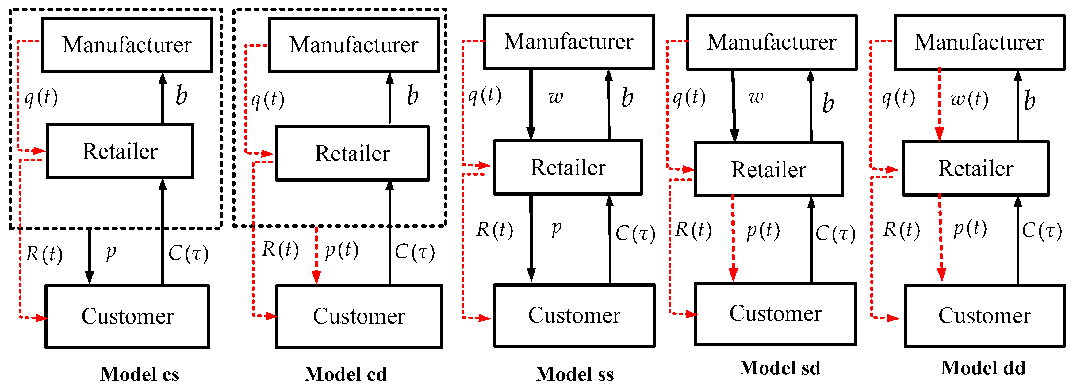
Since the reference quality is closely related with the product quality, the reference quality R(t) is always time-varying. Decentralized and centralized decision-making models are two predominant mainstreams in supply chain management [15,16,20]. Although the product quality and the reference quality invariably change with time, alternative pricing strategies can be selected for the manufacturer and the retailer-one is a time-varying pricing strategy and another is pricing statically. The static pricing strategy can be seen as a special case of the dynamic one in the decentralized model. Hence, four different patterns of the pricing strategies for the closed-loop supply chain are theoretically feasible. However, the retail price would also vary with the wholesale prices. Accordingly, it rarely happens in reality that the manufacturer takes a time-varying wholesale price, whereas the retailer adopts a uniform price. Hence, the model in which the manufacturer adopts a time-varying wholesale price, whereas the retailer applies a steady-state retail price is absolutely eliminated in our work. We obtain three different pricing strategies in the decentralized scenario and two distinct ones in the centralized scenario for the closed-loop supply chain shown in Figure 1.

In Figure 1, five models of the manufacturer and the retailer are listed, with the red and dotted downward line as the dynamic variables (q(t) represent product quality the retailer got from the manufacturer, R(t) represents reference quality the customer obtained from the retailer, and w(t) and p(t) represent the dynamic wholesale price and retail price, respectively), with the black and solid line as the static variables (C(τ) means the costs the manufacturer spent to collect the returned products from customer, b means the costs the manufacturer spent to retrieve the sold items from the retailer, and w and p represent the static wholesale price and retail price, respectively).

We derive a closed-loop supply chain with the retailer collecting the sold items, as the retailer is frequently exposed to the market as well as consumers, the used product was recovered by retailer and then transformed to the manufacturer with the price b. The production cost of the new product is c_m, and c_r denotes the cost of remanufacturing, producing a new product with a recycled item costs less than manufacturing a new one, we assume c_r < c_m and b + c_r < c_m [10]. Proposing that a fraction τ is controlled by the retailer and a higher τ means more difficult to recover, namely, it will cost more for the retailer to reach a greater proportion of recycled products, 0 < τ < 1, and τ = 0 denotes that the retailer will not take recycling policy.

Product quality is determined by some core components (e.g., camera pixels, memory size, battery capacity, CPU for mobile phone) for the products. These components have a series of quality levels and the qualified manufacturer applies different key ingredients to decide the product quality that makes product quality become a possible time-varying variable [5]. The performance of these critical components gradually declines so that they eventually stop working during product usage. The remanufacturing process is replacing the used components with the corresponding new ones. Hence, we assume that the remanufactured goods are as good as the brand-new products in quality [35].

3.3. Model Setting

Assuming that the product quality is observable by its features in the selling process, when deciding to purchase this product, consumers tend to evaluate product quality based on a benchmark, called reference quality. This product quality consumers perceived is affected through using some information, such as, consumers’ previous experience about this product, past product quality levels, and the quality of its competitive counterparts, etc. To obtain the reference quality, customers calculate the continuous weighted average of all the previous product quality. Similar to extant research [34,44], reference quality writes

$$R(t)=e^{-\theta t}[R_0+\theta {\displaystyle {\int }_0^t{e}^{\theta s}q(s)ds}]$$

(1)

where θ > 0 represents the continuous memory coefficient (or forgetting parameter) and R₀ denotes the initial reference quality at time t = 0. As such, solving the derivatives of R(t), that is dR(t)/dt or $\stackrel{•}{R(t)}$, we employ an exponential smoothing process of this historical quality to characterize the dynamics of reference quality, as follows, which is seen in research [16,27,45].

$$\stackrel{•}{R(t)}=\theta \left(q(t)-R(t)\right),R(0)=R_0\ge 0$$

(2)

Similar to previous literature [20,46], we now describe market demand, which is influenced by market capacity, retail price, product quality, and reference quality. The function of reference quality on market demand relies on the difference between product quality and reference quality, and the market demand function is given by:

$$D\left(p(t),q(t),R(t)\right)=\alpha -\beta p(t)+{\gamma }_{1}q(t)+{\gamma }_2\left(q(t)-R(t)\right)$$

(3)

where α ≥ 0 denotes market capacity, β ≥ 0 and γ₁ ≥ 0 represents the effects of retail price, and quality on current demand, respectively, γ₂ ≥ 0 captures the effect of the difference between product quality and reference quality on current sales.

The total costs for the whole supply chain composed of manufacturing/remanufacturing cost, quality cost undertaken by the manufacturer, and recovery cost owned by retailer. c_m and b + c_γ represent the unit cost of manufacturing and remanufacturing, respectively. In accordance with former literatures [45,47], a quadratic cost function about quality level is proposed below:

$$C(q)=\frac{k_1}{2}{q}^2(t)$$

(4)

The recovery cost mainly consists of fixed expenses in accord with returning fraction $\tau$ caused by early investment, such as establishing the recycling channel and enhancing customers’ awareness of recycling. Analogous to the extant literature [6,12,48], we obtain the following recovery cost function:

$$C(\tau )=\frac{k_2}{2}{\tau }^2$$

(5)

Follow [44], the objective functions of profits for the stakeholders, the manufacturer, and the retailer of a closed-loop supply chain are denoted, respectively, as follows:

$$J_M={\displaystyle {\int }_0^T\left\{\left(w(t)-c_m+\Delta \tau -b\tau \right)\left(\alpha -\beta p(t)+{\gamma }_{1}q(t)+{\gamma }_2\left(q(t)-R(t)\right)\right)-\frac{k_1}{2}q{(t)}^2\right\}dt}$$

(6)

$$J_R={\displaystyle {\int }_0^T\left\{\left(p(t)-w(t)+b\tau \right)\left(\alpha -\beta p(t)+{\gamma }_{1}q(t)+{\gamma }_2\left(q(t)-R(t)\right)\right)\right\}dt-\frac{k_2}{2}{\tau }^2}$$

(7)

4. Centralized Decision System Scenario

In the centralized case, the manufacturer and the retailer adopt various strategies to seek the maximal profit for the whole supply chain. The profit maximization problem in the centralized scenario can be given by:

$$\begin{array}{c}\underset{q(•),p(•)}{\max }{\displaystyle {\int }_0^T\left\{\left(p(t)-c_m+\Delta \tau \right)\left(\alpha -\beta p(t)+{\gamma }_{1}q(t)+{\gamma }_2\left(q(t)-R(t)\right)\right)-\frac{k_1}{2}q{(t)}^2\right\}dt-\frac{k_2}{2}{\tau }^2}\\ s.t.\stackrel{•}{R(t)}=\theta \left(q(t)-R(t)\right),R(0)=R_0\end{array}$$

(8)

We develop two cases in this section: one in which the closed-loop supply system applies a steady-state retail price, the other where the closed-loop supply system is pricing dynamically. Next, the optimal solutions about price, quality, and reference quality in both cases, are revealed, respectively.

4.1. The Static Price Model

When considering a uniform retail price, the centralized closed-loop supply chain system will maximize its profit function (7). Now, the following proposition depicts the optimum strategies on price, quality, and reference quality in the presence of pricing uniformly in such a closed-loop supply chain system. All the proofs of propositions and corollaries are disclosed in the Appendix for the sake of the readability of this paper.

Proposition 1.

By pricing statically, the equilibrium strategies on retail price, quality, and reference quality for the centralized closed-loop supply chain are revealed below:

$$p_{}^{cs}=\frac{(\alpha +(c_m-\Delta \tau )\beta )k_1\theta T+(c_m-\Delta \tau )M+k_1{\gamma }_2(e^{-\theta T}-1)R_0}{2\beta k_1\theta T+M}$$

(9)

$$q_{}^{cs}=\frac{(\alpha +(\Delta \tau -c_m)\beta )\theta T+{\gamma }_2(e^{-\theta T}-1)R_0}{2\beta k_1\theta T+M}({\gamma }_2{e}^{\theta (t-T)}+{\gamma }_1)$$

(10)

$$R(t)=R_0{e}^{-\theta t}+\frac{(\alpha +(\Delta \tau -c_m)\beta )\theta T+{\gamma }_2(e^{-\theta T}-1)R_0}{2\beta k_1\theta T+M}[({\gamma }_1(1-e^{-\theta t})+\frac{{\gamma }_2}{2}(e^{\theta (t-T)}-e^{-\theta (t+T)})]$$

(11)

where M denotes in the Appendix A.1.

4.2. The Dynamic Price Model

When considering a time-varying retail price, the centralized closed-loop supply chain system will maximize its profit function (7). Now, the following proposition describes the optimal strategies on price, quality, and reference quality in the context of pricing dynamically in such a closed-loop supply chain system.

Proposition 2.

By pricing dynamically, the equilibrium strategies on retail price, quality, and reference quality for the centralized closed-loop supply chain are displayed below:

$$R^{cd}(t)=h_1{e}^{r_{1}t}+h_2{e}^{r_{2}t}-B_1$$

(12)

$$\begin{array}{l}{p}^{cd}=\frac{k_1\alpha +(c_m-\Delta \tau )(\beta k_1-{({\gamma }_{{}^1}+{\gamma }_{{}^2})}^2)}{2k_1\beta -{({\gamma }_{{}^1}+{\gamma }_{{}^2})}^2}+\frac{({\gamma }_{{}^1}+{\gamma }_{{}^2})\theta }{2k_1\beta -{({\gamma }_{{}^1}+{\gamma }_{{}^2})}^2}(h_1\frac{N_1+\sqrt{N_1{}^2-2k_1{\gamma }_2{}^2\beta }}{2\beta \theta }{e}^{r_{1}t}\\ +h_2\frac{N_1-\sqrt{N_1{}^2-2k_1{\gamma }_2{}^2\beta }}{2\beta \theta }{e}^{r_{2}t}-A_1)-\frac{k_1{\gamma }_2}{2k_1\beta -{({\gamma }_{{}^1}+{\gamma }_{{}^2})}^2}(h_1{e}^{r_{1}t}+h_2{e}^{r_{2}t}-B_1)\end{array}$$

(13)

$$\begin{array}{l}{q}^{cd}=\frac{({\gamma }_{{}^1}+{\gamma }_{{}^2})(\alpha +(\Delta \tau -c_m)\beta )}{2k\beta -{({\gamma }_{{}^1}+{\gamma }_{{}^2})}^2}+\frac{2\theta \beta }{2k\beta -{({\gamma }_{{}^1}+{\gamma }_{{}^2})}^2}(h_1\frac{N_1+\sqrt{N_1{}^2-2k_1{\gamma }_2{}^2\beta }}{2\beta \theta }{e}^{r_{1}t}\\ +h_2\frac{N_1-\sqrt{N_1{}^2-2k_1{\gamma }_2{}^2\beta }}{2\beta \theta }{e}^{r_{2}t}-A_1)-\frac{({\gamma }_2{}^2+{\gamma }_{{}^1}{\gamma }_{{}^2})}{2k\beta -{({\gamma }_{{}^1}+{\gamma }_{{}^2})}^2}(h_1{e}^{r_{1}t}+h_2{e}^{r_{2}t}-B_1)\end{array}$$

(14)

where N₁, A₁, B₁, h_i, r_i, i = 1, 2 are characterized in Appendix A.2.

5. Decentralized Decision System Scenario

In the decentralized case, the manufacturer and the retailer regard maximizing their own interests as their decision criteria. Hence, the profit maximization problem in the decentralized case is shown in (14):

$$\begin{array}{l}\underset{q(•),w(•)}{\max }{\displaystyle {\int }_0^T\left\{\left(w(t)-c_m+\Delta \tau -b\tau \right)\left(\alpha -\beta p(t)+{\gamma }_{1}q(t)+{\gamma }_2\left(q(t)-R(t)\right)\right)-\frac{k_1}{2}q{(t)}^2\right\}dt}\\ \underset{p(•)}{\max }{\displaystyle {\int }_0^T\left\{\left(p(t)-w(t)+b\tau \right)\left(\alpha -\beta p(t)+{\gamma }_{1}q(t)+{\gamma }_2\left(q(t)-R(t)\right)\right)\right\}dt-\frac{k_2}{2}{\tau }^2}\\ s.t.\stackrel{•}{R(t)}=\theta \left(q(t)-R(t)\right),R(0)=R_0\end{array}$$

(15)

The equilibrium strategies on price, quality, and reference quality are presented, respectively, in triple scenarios according to distinct pricing strategies, viz., dynamically or uniformly. In the first scenario, both of the members of the closed-loop chain adopt a uniform price, the second is the manufacturer applies the steady-state wholesale price, whereas the time-varying retail price is adopted by the retailer and the third is both the stakeholders of the closed-loop chain employ the time-varying price in such a closed-loop supply chain.

5.1. The Static Wholesale Price and Retail Price Model

When considering the uniform wholesale and retail price, the stakeholders of the supply chain, the manufacturer and the retailer, will maximize their own profit function (14). Now, the following proposition characterizes the optimum strategies on price, quality, and reference quality in the presence of pricing uniformly in such a closed-loop supply chain system.

Proposition 3.

By pricing statically, the equilibrium strategies on wholesale price, retail price, quality, and reference quality for the manufacturer and the retailer are revealed below:

$$w^{ss}=\frac{2(\alpha +(2b\tau -\Delta \tau +c_m)\beta )\theta k_{1}T+(b\tau -\Delta \tau +c_m)M+2R_0{\gamma }_2{k}_1(e^{-\theta T}-1)}{4\beta k_1\theta T+M}$$

(16)

$$\begin{array}{l}{p}^{ss}=\frac{\alpha }{2\beta }+\frac{{\gamma }_2{R}_0(e^{-\theta T}-1)}{2\beta T\theta }+\frac{(\alpha +(\Delta \tau -c_m)\beta )\theta T+R_0{\gamma }_2(e^{-\theta T}-1)}{8{\beta }^2{k}_1\theta T^2+2\beta TM}{C}_1\\ +\frac{2(\alpha -(\Delta \tau -c_m)\beta )\theta k_{1}T-(\Delta \tau -c_m)M+2R_0{\gamma }_2{k}_1(e^{-\theta T}-1)}{8\beta k_1\theta T+2M}\end{array}$$

(17)

$$q^{ss}=\frac{(\alpha +(\Delta \tau -c_m)\beta )\theta T+R_0{\gamma }_2(e^{-\theta T}-1)}{4\beta k_1\theta T+M}({\gamma }_2{e}^{\theta (t-T)}+{\gamma }_1)$$

(18)

And the corresponding reference quality is:

$$R(t)=R_0{e}^{-\theta t}+\frac{(\alpha +(\Delta \tau -c_m)\beta )\theta T+R_0{\gamma }_2(e^{-\theta T}-1)}{4\beta k_1\theta T+M}[{\gamma }_1(1-e^{-\theta t})+\frac{{\gamma }_2}{2}(e^{\theta (t-T)}-e^{-\theta (t+T)})]$$

(19)

where C₁ denotes in Appendix A.3.

5.2. The Static Wholesale Price and Dynamic Retail Price Model

This model considers a uniform wholesale price and a dynamic retail price, the stakeholders of the supply chain, the manufacturer and the retailer, will maximize their own profit function (14). Now, the following proposition characterizes the optimum strategies on price, quality, and reference quality in the presence of pricing dynamically in such a closed-loop supply chain system.

Proposition 4.

Given a steady-state wholesale price and time-varying retail price, the equilibrium strategies on wholesale price, retail price, quality and reference quality for the manufacturer and the retailer are revealed below:

$$w^{sd}=\frac{2(\alpha +(2b\tau -\Delta \tau +c_m)\beta )\theta k_{1}T+(b\tau -\Delta \tau +c_m)M+2R_0{\gamma }_2{k}_1(e^{-\theta T}-1)}{4\beta k_1\theta T+M}$$

(20)

$$\begin{array}{l}{p}_{}^{sd}=\frac{\alpha -{\gamma }_2{R}_0{e}^{-\theta t}}{2\beta }+\frac{2(\alpha +(c_m-\Delta \tau )\beta )\theta k_{1}T+(c_m-\Delta \tau )M+2R_0{\gamma }_2{k}_1(e^{-\theta T}-1)}{8\beta k_1\theta T+2M}\\ +\frac{(\alpha +(\Delta \tau -c_m)\beta )\theta T+R_0{\gamma }_2(e^{-\theta T}-1)}{8{\beta }^2{k}_1\theta T+2\beta M}[({\gamma }_1+{\gamma }_2)({\gamma }_2{e}^{\theta (t-T)}+{\gamma }_1)\\ -{\gamma }_1{\gamma }_2(1-e^{-\theta t})-\frac{{\gamma }_2{}^2}{2}(e^{\theta (t-T)}-e^{-\theta (t+T)})]\end{array}$$

(21)

$$q_{}^{sd}=\frac{(\alpha +(\Delta \tau -c_m)\beta )\theta T+R_0{\gamma }_2(e^{-\theta T}-1)}{4\beta k_1\theta T+M}({\gamma }_2{e}^{\theta (t-T)}+{\gamma }_1)$$

(22)

$$R(t)=R_0{e}^{-\theta t}+\frac{(\alpha +(\Delta \tau -c_m)\beta )\theta T+R_0{\gamma }_2(e^{-\theta T}-1)}{4\beta k_1\theta T+M}[{\gamma }_1(1-e^{-\theta t})+\frac{{\gamma }_2}{2}(e^{\theta (t-T)}-e^{-\theta (t+T)})]$$

(23)

Corollary 1.

The optimum wholesale price, quality, reference quality and the benefits of the manufacturer in the “ss” model are equivalent to those in the “sd” model, that is,

$$w^{ss}=w^{sd}$$

(24)

$$q^{ss}(t)=q^{sd}(t)$$

(25)

$$R^{ss}(t)=R^{sd}(t)$$

(26)

$$J_M^{ss}=J_M^{sd}$$

(27)

Based on Corollary 1, the optimal wholesale price, quality, reference quality, and the benefits of the manufacturer will not be affected by the pricing strategy of the retailer, dynamically or statically, if the manufacturer applies a steady-state wholesale price.

5.3. The Dynamic Wholesale Price and Retail Price Model

When considering the dynamic wholesale and retail price, the stakeholders of the supply chain, the manufacturer and the retailer, will maximize their own profit function (14). Now, the following proposition characterizes the optimum strategies on price, quality, and reference quality in the presence of pricing dynamically in such a closed-loop supply chain system.

Proposition 5.

By pricing dynamically, the equilibrium strategies on wholesale price, retail price, quality, and reference quality for the manufacturer and the retailer are disclosed below:

$$\begin{array}{l}{w}_{}^{dd}=\frac{2k_1(\alpha +\beta (c_m+2b\tau -\Delta \tau ))+{({\gamma }_1+{\gamma }_2)}^2(\Delta \tau -b\tau -c_m)}{4\beta k_1-{({\gamma }_1+{\gamma }_2)}^2}-\frac{2k_1{\gamma }_2}{4\beta k_1-{({\gamma }_1+{\gamma }_2)}^2}(h_3{e}^{r_{3}t}+h_4{e}^{r_{4}t}\\ -B_2)+\frac{2\beta \theta ({\gamma }_1+{\gamma }_2)}{4\beta k_1-{({\gamma }_1+{\gamma }_2)}^2}(h_3\frac{N_2+\sqrt{N_2{}^2-4k_1{\gamma }_2{}^2\beta }}{4\beta \theta }{e}^{r_{3}t}+h_4\frac{N_2-\sqrt{N_2{}^2-4k_1{\gamma }_2{}^2\beta }}{4\beta \theta }{e}^{r_{4}t}-A_2)\end{array}$$

(28)

$$\begin{array}{l}{p}_{}^{dd}=\frac{(2+\beta )({\gamma }_1+{\gamma }_2)\theta }{4\beta k_1-{({\gamma }_1+{\gamma }_2)}^2}(h_3\frac{N_2+\sqrt{N_2{}^2-4k_1{\gamma }_2{}^2\beta }}{4\beta \theta }{e}^{r_{3}t}+h_4\frac{N_2-\sqrt{N_2{}^2-4k_1{\gamma }_2{}^2\beta }}{4\beta \theta }{e}^{r_{4}t}-A_2)\\ +\frac{k_1(3\alpha +\beta (c_m-\Delta \tau ))+(\Delta \tau -c_m){({\gamma }_1+{\gamma }_2)}^2)}{4\beta k_1-{({\gamma }_1+{\gamma }_2)}^2}-\frac{3k_1{\gamma }_2}{4\beta k_1-{({\gamma }_1+{\gamma }_2)}^2}(h_3{e}^{r_{3}t}+h_4{e}^{r_{4}t}-B_2)\end{array}$$

(29)

$$\begin{array}{l}{q}_{}^{dd}=\frac{({\gamma }_1+{\gamma }_2)(\alpha +\beta (\Delta \tau -c_m))}{4\beta k_1-{({\gamma }_1+{\gamma }_2)}^2}+\frac{4\beta \theta }{4\beta k_1-{({\gamma }_1+{\gamma }_2)}^2}(h_3\frac{N_2+\sqrt{N_2{}^2-4k_1{\gamma }_2{}^2\beta }}{4\beta \theta }{e}^{r_{3}t}\\ +h_4\frac{N_2-\sqrt{N_2{}^2-4k_1{\gamma }_2{}^2\beta }}{4\beta \theta }{e}^{r_{4}t}-A_2)-\frac{({\gamma }_2{}^2+{\gamma }_1{\gamma }_2)}{4\beta k_1-{({\gamma }_1+{\gamma }_2)}^2}(h_3{e}^{r_{3}t}+h_4{e}^{r_{4}t}-B_2)\end{array}$$

(30)

$$R^{dd}(t)=h_3{e}^{r_{3}t}+h_4{e}^{r_{4}t}-B_2$$

(31)

where N₂, A₂, B₂, h_i, r_i, i = 3, 4 are characterized in Appendix A.6.

Proposition 6.

According to Propositions 1–5, the demand of the product in which the system adopts the static and dynamic pricing strategies in centralized and decentralized case are presented as follows respectively:

$$\begin{array}{l}{D}^{cs}=\frac{(\alpha +(\Delta \tau -c_m)\beta )\theta T+{\gamma }_2(e^{-\theta T}-1)R_0}{2\beta k_1\theta T+M}{C}_1+\alpha T+\frac{{\gamma }_2{R}_0(e^{-\theta T}-1)}{\theta }\\ -\beta T\frac{(\alpha +(c_m-\Delta \tau )\beta )k_1\theta T+(c_m-\Delta \tau )M+k_1{\gamma }_2(e^{-\theta T}-1)R_0}{2\beta k_1\theta T+M}\end{array}$$

(32)

$$\begin{array}{l}{D}^{cd}=\frac{k_1\beta (\alpha -\beta (c_m-\Delta \tau ))}{2k_1\beta -{({\gamma }_{{}^1}+{\gamma }_{{}^2})}^2}T-\frac{{\gamma }_2{k}_1\beta }{2k_1\beta -{({\gamma }_{{}^1}+{\gamma }_{{}^2})}^2}(h_1\frac{e^{r_{1}t}-1}{r_1}+h_2\frac{e^{r_{2}T}-1}{r_2}-B_{1}T)\\ +\frac{\beta \theta ({\gamma }_{{}^1}+{\gamma }_{{}^2})}{2k_1\beta -{({\gamma }_{{}^1}+{\gamma }_{{}^2})}^2}(\frac{h_1(N_1+\sqrt{N_1{}^2-4k_1{\gamma }_2{}^2\beta })(e^{r_{1}t}-1)}{4\beta \theta r_1}+\frac{h_2(N_1-\sqrt{N_1{}^2-4k_1{\gamma }_2{}^2\beta })(e^{r_{2}T}-1)}{4\beta \theta r_2}-A_{1}T)\end{array}$$

(33)

$$\begin{array}{l}{D}^{ss}=D^{sd}=\frac{\alpha T}{2}+\frac{{\gamma }_2{R}_0(e^{-\theta T}-1)}{2\theta }+\frac{(\alpha +(\Delta \tau -c_m)\beta )\theta T+R_0{\gamma }_2(e^{-\theta T}-1)}{8\beta k_1\theta T+2M}{C}_1\\ -\frac{2(\alpha -(\Delta \tau -c_m)\beta )\beta \theta k_1{T}^2-(\Delta \tau -c_m)\beta MT+2T{R}_0{\gamma }_2{k}_1\beta (e^{-\theta T}-1)}{8\beta k_1\theta T+2M}\end{array}$$

(34)

$$\begin{array}{l}{D}^{dd}=-\frac{\beta k_1{\gamma }_2}{4\beta k_1-{({\gamma }_1+{\gamma }_2)}^2}(h_3\frac{e^{r_{3}t}-1}{r_3}+h_2\frac{e^{r_{4}T}-1}{r_4}-B_{2}T)+\beta T\frac{k_1(\alpha -\beta (c_m-\Delta \tau ))}{4\beta k_1-{({\gamma }_1+{\gamma }_2)}^2}+\\ \frac{\beta ({\gamma }_1+{\gamma }_2)}{4\beta k_1-{({\gamma }_1+{\gamma }_2)}^2}(\frac{h_3(N_2+\sqrt{N_2{}^2-4k_1{\gamma }_2{}^2\beta })(e^{r_{3}t}-1)}{4\beta \theta r_3}+\frac{h_4(N_2-\sqrt{N_2{}^2-4k_1{\gamma }_2{}^2\beta })(e^{r_{4}T}-1)}{4\beta \theta r_4}-A_{2}T)\end{array}$$

(35)

6. Numerical Examples

In this section, we firstly investigate the flexibility analysis of several of the significance parameters to find out how they affect the equilibrium strategies and then derive numerical examples to examine the feasibility and effectiveness of our work. Finally, we explore the optimal recycling policy for the CLSC.

6.1. Sensitivity Analysis

To reveal the impacts of some parameters on optimal strategies, the specific parameter settings are α = 30, β = 0.6, γ₁ = 0.7, γ₂ = 0.5, θ = 0.2, R₀ = 5, b = 2, k₁ = 2, k₂ = 3, τ = 0.3, T = 10, according to previous researches in reference quality [46,49] and closed-loop supply chain [5,15,50,51].

We evaluate the flexibility analysis of several of the importance parameters, for instance, β, θ, γ₁ and γ₂ to study their influences on revenues for supply chain and its members in each case, which are shown in

Table 3. Sensitivity for profits of decision variables β, θ, γ₁ and γ₂.

		${\mathit{J}}_{}^{\mathit{c}\mathit{s}}$	${\mathit{J}}_{}^{\mathit{c}\mathit{d}}$	${\mathit{J}}_{}^{\mathit{s}\mathit{s}}$	${\mathit{J}}_{}^{\mathit{s}\mathit{d}}$	${\mathit{J}}_{}^{\mathit{d}\mathit{d}}$	${\mathit{J}}_{\mathit{M}}^{\mathit{s}\mathit{s}}$	${\mathit{J}}_{\mathit{M}}^{\mathit{s}\mathit{d}}$	${\mathit{J}}_{\mathit{M}}^{\mathit{d}\mathit{d}}$	${\mathit{J}}_{\mathit{R}}^{\mathit{s}\mathit{s}}$	${\mathit{J}}_{\mathit{R}}^{\mathit{s}\mathit{d}}$	${\mathit{J}}_{\mathit{R}}^{\mathit{d}\mathit{d}}$
$\beta$	0.2	5584.4	5934.2	3732.5	3975.2	4060.6	2436.4	2436.4	2674.5	1296.7	1305.9	1396.6
	0.4	2416.7	2443.3	1593.8	1708.7	1755.7	1051.6	1051.6	1161.8	542.75	547.6	594.5
	0.6	1433.6	1437.4	943.9	1017.0	1048.2	625.1	625.1	695.5	319.41	322.7	353.3
	0.8	963.1	963.5	632.4	684.75	707.6	419.5	419.5	470.1	213.40	215.9	238.0
$\theta$	0.2	1433.6	1437.4	943.9	1017.0	1048.2	625.0	625.0	695.5	319.41	322.7	353.3
	0.4	1471.7	1473.9	960.0	1043.1	1078.2	636.4	636.4	716.1	324.2	328.4	362.6
	0.6	1502.9	1505.8	993.3	1071.0	1103.6	658.7	658.7	733.2	335.2	339.2	371.0
	0.8	1527.8	1531.5	1025.6	1095.1	1123.8	680.2	680.2	746.7	346.0	349.5	377.6
${\gamma }_1$	0.4	1390.9	1390.1	922.6	995.7	1027.8	613.6	613.6	684.2	309.5	312.9	344.1
	0.5	1404.1	1403.9	928.83	1001.9	1033.7	617.0	617.0	687.5	312.4	315.7	346.8
	0.6	1418.4	1419.7	935.9	1009.0	1040.6	620.8	620.8	691.3	315.7	319.0	349.8
	0.7	1433.6	1437.4	943.9	1017.0	1048.2	625.0	625.0	695.5	319.4	322.7	353.3
${\gamma }_2$	0.3	1528.1	1534.0	1064.6	1108.0	1127.8	705.7	705.7	748.3	359.4	360.6	380.1
	0.4	1480.1	1479.5	1003.8	1062.0	1087.8	665.1	665.1	721.7	339.3	341.4	366.6
	0.5	1433.6	1437.4	943.9	1017.0	1048.2	625.0	625.0	695.5	319.4	322.7	353.3
	0.6	1388.5	1385.2	884.7	972.85	1007.2	585.4	585.4	674.3	299.8	304.6	334.1

.

When comparing time-varying and steady-state pricing strategies, an apparent result suggests that the benefits of a centralized closed-loop supply chain are invariably much better than those of a decentralized one. The supply chain achieves more profitable revenue with dynamic pricing than with pricing statically both in the centralized and decentralized form, that is, J^cd > J^cs > J^dd > J^sd > J^ss. It means that the centralized form and the dynamic pricing benefit the whole supply chain. In the centralized form, the retailer and the manufacturer obtain more profitable revenue in dynamic pricing than in uniform pricing, namely, $J_M^{dd}>J_M^{ss}=J_M^{sd},J_R^{dd}>J_R^{sd}>J_R^{ss}$.

From Table 2, we can find that the revenues of the whole supply chain, the manufacturer and the retailer constantly grow with γ₁ and θ increasing with whatever pricing strategy is adopted. Nevertheless, the higher β and γ₂ create less benefits for the stakeholders of the closed-loop supply chain. It signifies that the whole closed-loop supply chain and its members will obtain the most benefits if quality effect γ₁ and the impact of continuous memory coefficient of reference quality θ are higher, while the marginal contribution of the difference between quality and reference quality γ₂ and the price elasticity coefficient β are lower.

6.2. The Numerical Example on Equilibrium Strategies

Next, due to Propositions 1 and 2, the equilibrium strategies about quality, reference quality, and price for the whole supply chain are acquired in the centralized model. By applying Propositions 3–5, we derive the optimum policies on quality, reference quality, and wholesale and retail price for the manufacturer and the retailer in the decentralized case, respectively, which are denoted in Figure 2, Figure 3 and Figure 4 below.

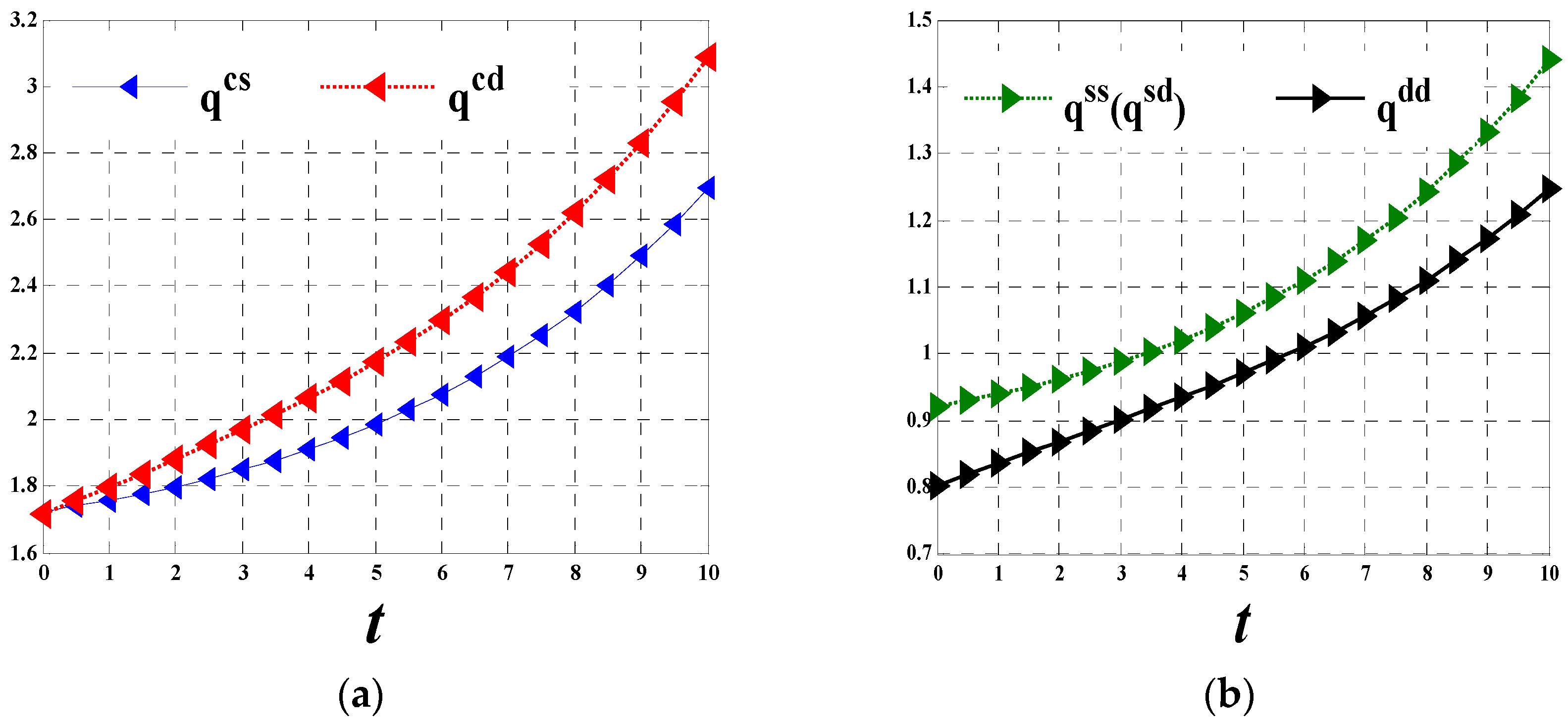
An obvious result shown in Figure 2 is that regardless of case, the quality increases in the entire planning horizon. It indicates that the manufacturer would continuously enlarge the quality input regardless of what pricing policy the manufacturer and the retailer will adopt. The product quality in which the manufacturer takes a time-varying price is a little bit higher when compared with that in which the manufacturer adopts a steady-state price in both the centralized and decentralized scenarios. The manufacturer will put much more investment in product quality in the centralized case than in the decentralized scenario, where the manufacturer and the retailer are pricing dynamically and in the case where they are pricing uniformly.

It visibly signifies that time-varying pricing and the centralized decision form are propitious to product quality. Dynamically pricing strategies require a high level of input to continuously improve product quality. However, the improvement of product quality is not accomplished overnight, so that enterprises preparing for adopting dynamic pricing strategies should do some basic research and development work regarding product quality in advance.

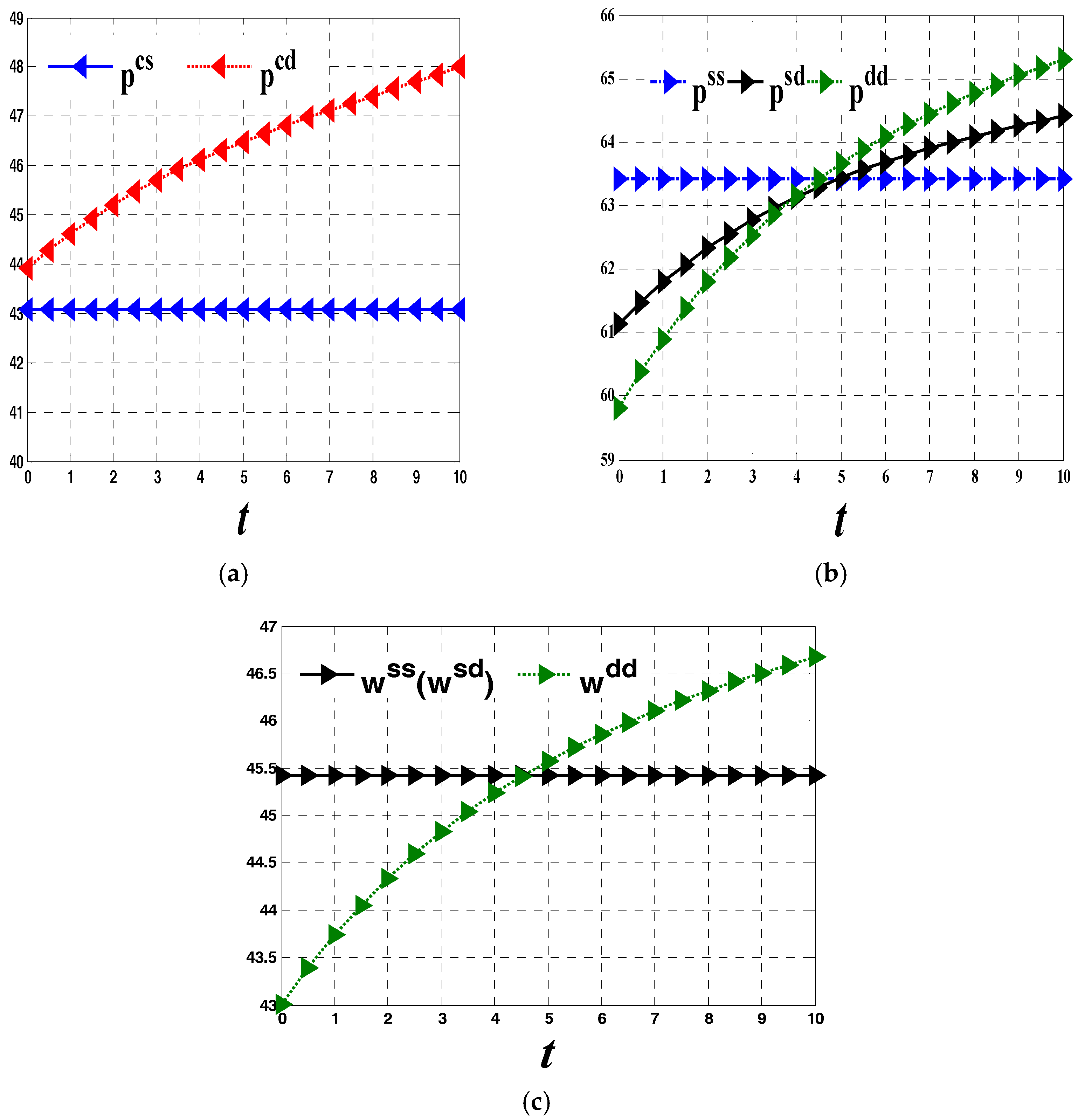
Clearly, the Figure 3 shows that the retail price and the wholesale price always grow throughout the cycle in dynamic pricing cases. In the centralized case, the retail price in which the supply chain adopts dynamic pricing strategies outclasses that with the supply chain pricing statically. The peak retail and wholesale price belongs to the case where the supply chain is pricing statically in the first semi-period, and in which both the members of the supply chain adopt a time-varying price in the last part in decentralized case. We can infer that dynamic prices exceed static ones and these differences are increasingly large within a longer planning horizon, which firmly means dynamic pricing is more suitable for a long-term cooperative supply chain.

When comparing quality and price strategies presented in Figure 2 and Figure 3, quality level and retail price continue to grow in a period when adopting dynamic pricing strategy both in the decentralized and centralized cases. It suggests that dynamic pricing strategies, that is, a policy with gradually increased high-quality product and higher and higher price, will lead to an upscale brand famous for top-level quality and peak price throughout its life-cycle among like products. Dynamic pricing strategies would be more applicable for those companies identified as “high-end firms”.

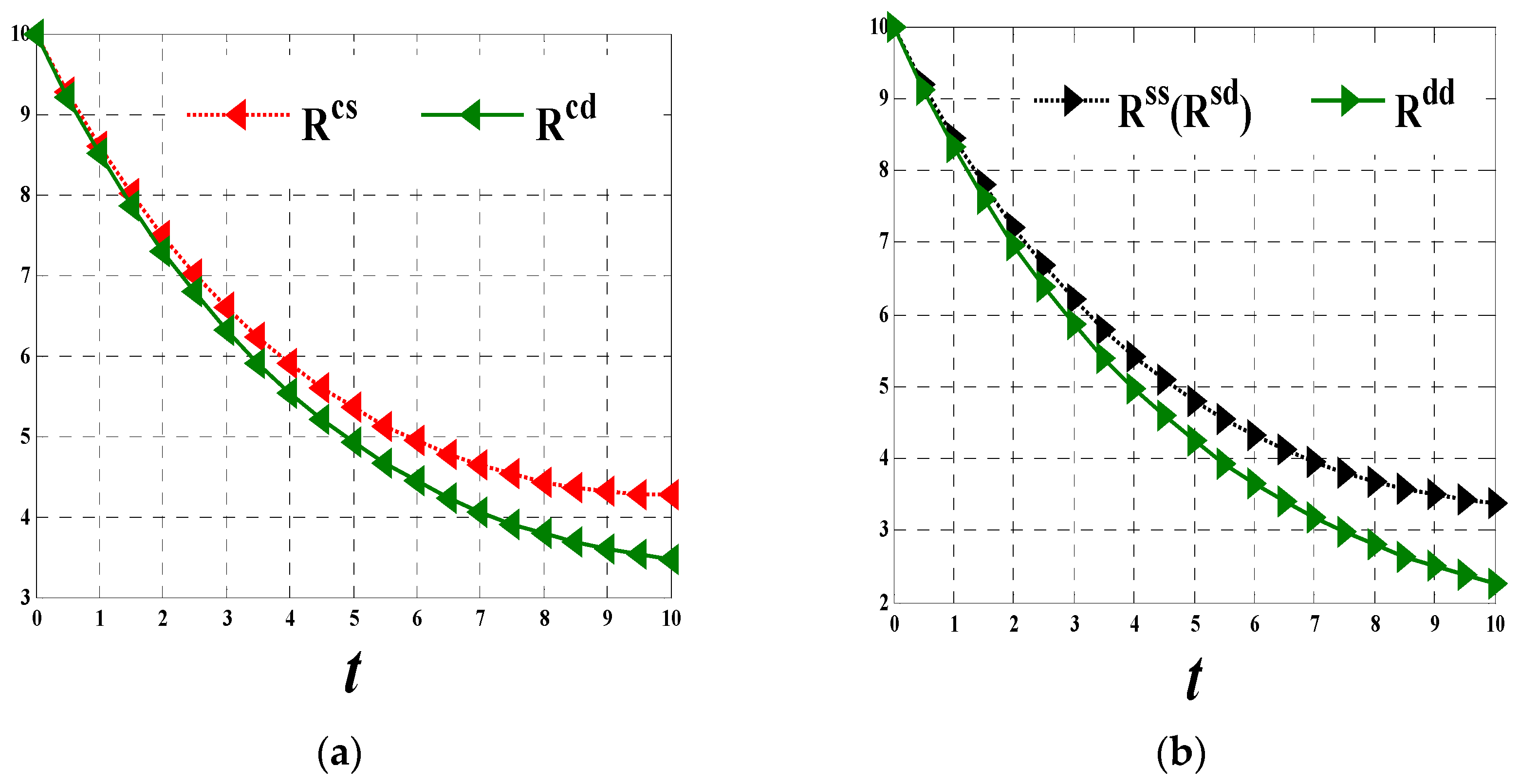
As it obviously depicted in Figure 4, the reference quality where the system adopts a uniform price is slightly smaller than that with the system pricing dynamically. The reference quality presents an overall tendency to decline as time goes by in all distinct pricing strategies in the entire planning horizon. The reason can be found in the first beginning, q(t) < R(t), which means $\stackrel{•}{R}(t)<0$ and derivative of R(t) less than zero, that is, the reference quality decreased. An interesting inference can be obtained that R(t) will increase in the long term for q(t) growing and R(t) decreasing, once q(t) > R(t) that means $\stackrel{•}{R}(t)>0$ and derivative of R(t) more than zero, which lead the reference quality to a constant growth.

It suggests that the consumers’ reference quality is in accord with product quality. Due to reference quality effects, though the manufacturer has been improving the product quality, the product quality consumers really apperceived decreased firstly and then increased in the long term. In other words, once the manufacturer decides to adopt dynamic pricing strategies and produce a continuously high-quality product, the reference quality perceived by customers decreases first and eventually grows with the manufacturer persistently improving product quality, which results in a virtuous cycle where the quality and the reference quality promote and rise mutually.

Since the product quality is less than the reference quality and the gap decreases as time goes on, the effect the gap has on current demand increases and the total demand of the product constantly grows with a static pricing strategy, according to Equation (2). In dynamic pricing, the product quality and the difference between the product quality and the reference quality have a positive effect on current demand, whereas the gradually increasing price has a negative effect on demand. The relationship between the general demand and time is unclear, however, we can infer that total demand is declining in a long enough planning horizon due to a substantially increased price from Figure 3 and Figure 4.

The above strategies about retail price, wholesale price, and product quality are the best solutions where the retailer takes the recycling policy. Note that the recycling cost is fixed with the rate of recycling and this fraction does not work on the equilibrium strategies mentioned before; we can obtain the optimal strategies where the manufacturer takes recycling policy represented in Corollary 2.

Corollary 2.

Let b = 0, the Propositions 1–5, are the optimal pricing strategies in which the manufacturer takes recycling policy.

According to Corollary 2, retail price, wholesale price, and product quality strategies in corresponding scenarios with the manufacturer taking the recycling policy can be regarded as a special case of that with the retailer adopting the recycling policy. For the manufacturer, it will be responsible for the recycling activities where the recycling cost is lower than expense spending on the transaction cost to the retailer, that is, k₂τ²/2 < bτD(t).

6.3. Analysis of the Optimal Recycling Fraction

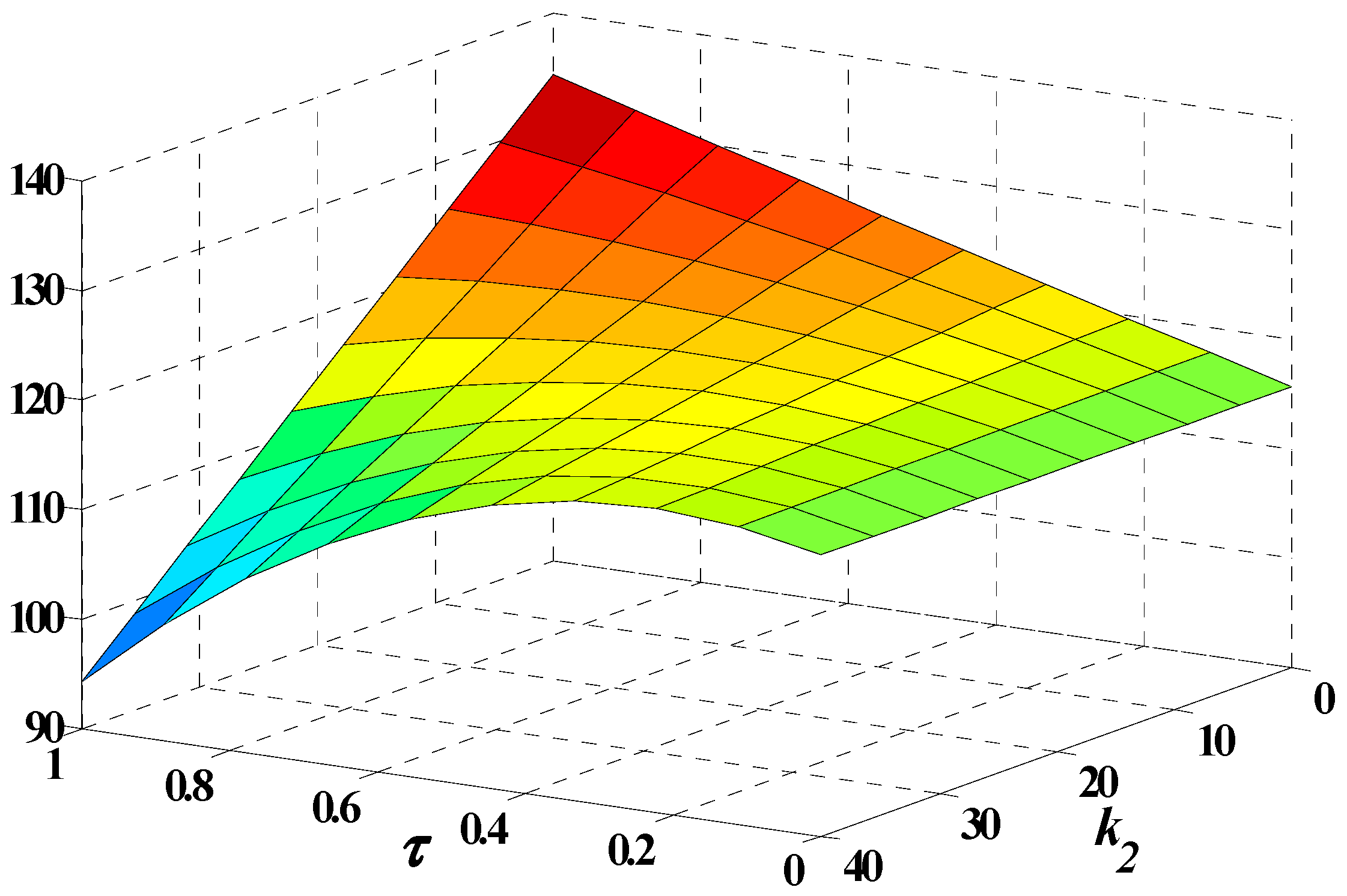
Especially, we discuss the influence the recovery fraction τ has on the whole supply chain and its members. It should be considered that the profits for all of the participants increase gradually with τ increases. Actually, this summary only works with specific parameter k₂. A higher τ means saving more manufacturing costs, but leading to additional recovery costs simultaneously. The retailer benefits more with a high level of recovery where the rate of increasing sales is larger than that of the growing recovery cost. Consequently, the impact the recovery fraction has on the profit is mainly dependent on the recovery cost coefficient k₂.

The relation between τ and profits for members of the supply chain vary considerably in precise value of k₂. Applying Proposition 3, taking τ^ss as an example, we drive the profit of the retailer with the recovery cost coefficient k₂ and the recycling fraction coefficient τ gradually increasing at the same time.

Figure 5 depicts that the relationship between the profit for the retailer and the recycling ratio τ is not regular, namely, the retailer will get a continuously increasing profit with τ gradually increasing, in which k₂ is less than a specific range, and an increased then declining revenue with τ increasingly growing where k₂ is beyond that range. In dynamic pricing strategies, the recycling fraction should be determined by recovery cost, the retailer should take a higher recycling rate when the recovery cost is low, while adopting a lower recycling ratio when the recovery cost is high. The optimal recycling fraction is specific to a given recovery cost from Figure 5; to gain the concrete relationship between recycling fraction and the recycling cost, we get Corollary 3.

Corollary 3.

No matter in which case, as a rational retailer, they would take the return contract only if that will make them more benefit than not accepting the recycling policy. Let ∆J denote the additional profit for the retailer generated by taking the recovery policy; the necessary condition for the retailer to adopt the recycling contract is ∆J > 0. Taking “ss” state as an example, hence, the most appropriate recycling fraction must meet the following statement:

$$\tau =\{\begin{array}{c}0,k_2>\frac{2\beta \theta k_{1}T+M+\theta C_1}{\Delta \beta bT(4\beta k_1\theta T+M)}\\ \begin{array}{l}\frac{2bH}{\Delta \beta bT(4\beta \theta k_{1}T+2M+2\theta C_1)-k_2(8\beta k_1\theta T+2M)},\\ k_2\in (\frac{2b\left(\beta T(C_1\Delta \theta +2\beta \Delta \theta k_{1}T+\Delta M)-H\right)}{8\beta k_1\theta T+2M},\frac{2\beta \theta k_{1}T+M+\theta C_1}{\Delta \beta bT(4\beta k_1\theta T+M)})\\ \end{array}\\ 1,A\in (0,\frac{2b\left(\beta C_1\Delta \theta T+2{\beta }^2\Delta \theta k_1{T}^2+\beta \Delta MT-H\right)}{8\beta k_1\theta T+2M})\end{array}$$

(36)

where H denotes in the Appendix A.8.

As a rational retailer, an appropriate return policy can be based on a given recycling cost coefficient where the closed-loop supply chain adopts dynamic pricing and quality strategies. The best recycling fraction and the recovery cost coefficient are inversely proportional from Corollary 3. To be economically profitable, the retailer will reject the recycling contract no matter which recovery fraction if the recycling cost is high enough, while the retailer should collect all of the sold products with a much lower recycling cost. It is impossible for the retailer to recycle one hundred percent of the used items. To reach a higher fraction of recycling and a lower recovery cost coefficient, the simplicity and low cost of recycling is essential for the retailer in practice.

However, the profit of the manufacturer continuously increases with τ growth. To get higher revenues, the manufacturer wants the retailer to take a higher rate of recovering used goods which indicates a lower recycling cost coefficient is urgently needed for the retailer and the manufacturer. The manufacturer should make contributions, such as helping the retailer to set up and enlarge the recovery channel or advocate more in recycling among consumers, to make the retailer get a smaller k₂, so that the retailer will invest more in returning the used goods, which would lead to a win-win situation for both of them.

7. Conclusions

In this paper, we employ a Stackelberg game between a manufacturer and a retailer in a closed-loop supply chain. The manufacturer is a leader who settles the quality level and the wholesale price while the retailer is a follower who determines the retail price in the Stackelberg game. The main purpose of our work is to investigate different pricing strategies in the context of dynamic quality characterized by reference quality effects for such a closed-loop supply chain. Particularly, we determined the optimal strategies in several cases: one is where the whole supply chain adopts static and dynamic pricing strategies in a centralized scenario; the other one is either, neither, or both the manufacturer and the retailer take time-varying pricing strategies, respectively, in a decentralized case. In addition, the optimal recycling fractions for such a closed-loop supply chain in each scenario are also discussed throughout this paper.

Furthermore, the primary results of our work stated below are available by investigating numerical examples and flexibility analysis: (1) The profits where the supply chain take pricing decisions in a centralized case is better than profits in a decentralized scenario no matter whether pricing dynamically or statically. (2) The case in which the whole supply chain takes a time-varying price is better than the case in which either or neither of the manufacturer and the retailer price dynamically regardless of being in a centralized or decentralized model. (3) The reference quality move towards the product quality and dynamic pricing strategies are suitable more for the long term, according to comprehensive effects between price and demand. (4) The profits of the whole supply chain, the manufacturer, and the retailer always grow with γ₁ and θ increasing, while they decrease with β and γ₂ growing. (5) The best recycling fraction is obtained for the whole supply chain in all distinct cases.

Some practical implications for industry according to the results are as follows. Firstly, the effects of different price-making models on the manufacturer’s profit are consistent with that on the retailer’s. The centralized model will make the closed-loop supply chain and its members achieve more revenues than a dynamic pricing strategy. It signifies that a dynamic pricing strategy with reference quality effects works more on a cooperative closed-loop supply chain.

Secondly, the manufacturer should continuously improve product quality no matter which pricing strategy the retailer and the manufacturer would make with reference quality effects. As for pricing statically, including the static wholesale price and the static retail price, the closed-loop system and its members could achieve less revenue than that with dynamic pricing; the gap of profit would enlarge over a longer term. It is far more likely that the manufacturer and the retailer will take the dynamic pricing strategies from a far-sighted perspective.

Dynamic quality and dynamic price are then promoted mutually, namely, dynamic pricing with reference quality effects is a policy with gradually increasing high-quality product with a higher price, will lead to an upscale brand throughout its life-cycle among its counterparts. Meanwhile, a dynamic pricing strategy with reference quality requires a high level of continuously improving product quality in the long term, which makes it more suitable for qualified companies to promote product quality increasingly or innovation-oriented firms.

Fourthly, these coefficients play an important role in the profits of the closed-loop system even in determining whether the manufacturer and the retailer choose to adopt the dynamic pricing strategy. Specifically, when customers are more sensitive to the product quality, when the memory coefficient of reference quality is higher, or when customers are less sensitive to the quality gap, when price elasticity coefficient is lower, the manufacturer and the retailer would be more willing to adopt these kinds of pricing strategies with reference quality. Therefore, it suggests that realizing some important parameters for the manufacturer and the retailer before producing products is useful in deciding the optimal pricing strategy.

Finally, the best recycling fraction is not affected by the dynamic decision-making model and proved to be uniform for the retailer in all of the distinct cases throughout the cycle. Since a higher recovery ratio is much more beneficial to the manufacturer, the manufacturer could make some efforts or pay added profit to the retailer to stimulate getting more used products returned.

Though this study has identified some important managerial insights, there are several directions worth investigating in further research. Initially, it would be meaningful to consider a distinct product system, including new product and remanufactured ones with different quality levels in which the whole supply chain and its members take a steady-state and time-varying pricing strategies, respectively. Then, the available extension of our study would be to investigate what impact the recovery policy has on the whole supply chain and its members in which the recycling fraction is a state variable. Lastly, some comprehensive contracts can be adopted, such as revenue sharing contracts and quantity discount contracts, to the closed-loop supply chain when making dynamic decisions.