Study on the Relationship between Land Transport and Economic Growth in Xinjiang

Abstract

Xinjiang’s land transport network is mainly comprised of highways and railways. Using statistical data from 1985 to 2015, this study applies the Lotka-Volterra model to investigate the competitive interactions among highway transport, railway transport, and the regional economy of Xinjiang. We can draw the following conclusions: First, highway mileage, highway passenger transportation, and railway freight transportation have played a significant role in promoting the development of the national economy in Xinjiang, while the latter has weakened highway passenger transportation and promoted the growth of the added value of transportation industry (AVTI), railway mileage, and railway passenger transportation. Second, highway passenger transportation enhances the development of railway passenger transportation, while railway freight transportation has played the same role in the development of highway freight transportation. Third, the increase in AVTI will increase total population, but both may have a negative impact on the national economy in the short term. Fourth, there is no significant relationship between the economy and transportation investment.

1. Introduction

In recent years, with the rapid economic development of society, it is increasingly more convenient for people to travel. Travel modes tend to be diversified, but the most common ways to travel are by highway and rail transport. Promoting and influencing the growth of the national economy by fully developing the advantages of highway and rail transport while achieving sustainable development between the transport industry and the national economy have been proven to be hot topics in recent research.

The relationship between the national economy and transportation seems complex because these two parameters form a dynamic system made up of a variety of factors, and these factors are interdependent and interact with each other when the system is operating. The mainstream view in ongoing research is that the national economy and transportation complement each other; transportation is not just a condition of regional development, but also a result of it [1,2,3]. Some scholars have empirically proven the driving effects of transportation and transportation investment on economic growth. Other research has shown that there is a long-term equilibrium relationship between freight volume and gross domestic product (GDP), and that transportation can promote the development of the whole national economy [4]. With economic development, rapidly expanding markets make the region’s economy more closely linked, placing higher demands on transportation. Economic development has brought a great deal of financial support to the transportation industry. However, the relationship between economic development and transportation is inconsistent because of geographical conditions, social environments, and national policy changes [5,6].

Mehmet et al. [7] investigates the Granger-causality relationship between income and transportation in EU-15 countries using a panel data set covering the period 1970–2008. Their findings indicate that the dominant type of Granger-causality is bidirectional. Instances of one-way or no Granger-causality were found to correspond with countries with the lowest income per capita ranks in 1970 and/or in 2008. Michael and David [8] test for mutual causality between the growth of road networks and changes in county-level population and employment using a panel data set containing observations of road mileage by type for all Minnesota counties over the period 1988 to 2007. The results indicate that causality runs in both directions between population and local road networks, while no evidence of causality in either direction is found for networks and local employment; these findings are evidence of the weakening influence of road networks on location.

On the other hand, there are some studies that try to explain the economic impact of transportation. For example, through the decomposition of the decoupling index of road freight traffic, Kveiborg and Fosgerau [9] find that the use of large vehicles, larger truckloads, and fewer empty loads are the most important drivers of economic growth. Li et al. [10] found that highway passenger turnover, annual average quality ratings of highways, and the rate of cement highways to administrative villages are the three primary factors that should be focused on in the future. Their findings also show that the development of highway traffic is closely related to the speed of economic development and transportation investment.

With the ‘Belt and Road Initiative’ proposed in China, in Xinjiang, which is located in the northwest border area, the transportation industry has received increasingly more unprecedented capital investment and technical support. Therefore, the relationship between Xinjiang’s economic development and the transportation infrastructure has obvious political implications. Domestic scholars also have done a lot of basic work, which provides a good reference for future research. Feng [11] and Xu [12] analyzed the contribution of highway transportation to the development of Xinjiang’s national economy and Xinjiang production and construction forces. The results showed that highway transportation has a positive effect on the promotion of social employment and economic growth. Zhu [13] studied the relationship between regional transportation and economic development in southern Xinjiang from 1999 to 2009, and predicted that their development trend will change from lagging growth to leading growth between 2010 and 2020. Zhang et al. [14] found that highway transportation’s contribution to Xinjiang’s economic growth is on a path of sustained and rapid growth over time, and that railway and aviation transportation contributed more slowly to economic growth.

These studies on transportation and economic development mostly focus on the macro scale, and there is less study of the competition between the national economy and land transport. To systematically investigate the interaction between land transport and Xinjiang’s national economy, we suggest a triangular Lotka-Volterra [15,16] competition model for sustainable development (LV-COMSUD). Invented from predator-prey relationship researches, the LV-COMSUD model treats land transportation, GDP and other parameters as dynamic system’s components, and examines their interactions applying a set of ordinary differential equations in a general form of competing species. This model provides the advancement and research of a transportation development planning basis and a brand new standpoint. In particular, LV-COMSUD seeks to identify the requisite activities for advancing the coordinated evolution of transportation’s distinct modes, and promoting and affecting the national economy together.

2. Study Area

Xinjiang is an arid zone that is affected by the temperate continental climate. The features of this wide geographical area include rich reserves of resources, ethnic minorities, and a weak economic foundation [4]. Xinjiang’s GDP in 2015 was 932.48 billion, only accounting for 1.4% of China’s GDP. In the same area, the GDP of Shanxi Province in the northwest region of China was 1821.26 billion yuan, while Xinjiang was only 51.7% of its GDP. Xinjiang, as China’s Western portal, has 111 border lines in five of eight bordering countries surrounding this region. It is China’s gateway to Central Asia, West Asia, Southwest Asia, Europe, and Africa [17]. Xinjiang has played an important role in China’s national economic development, social stability, national unity, and national security.

During the “Twelve-Five” period, land transportation in Xinjiang has seen significant development; 250 billion yuan (70 billion for railway and about 180 billion for highways) have been invested in land transportation. By the end of 2015, there were 5789 km of railway operating in Xinjiang, an increase of 1486 km compared with the end of the “Eleventh Five-Year”. The total distance of highways reached 176,000 km, an increase of 23,000 km compared with the end of the “Eleventh Five-Year” [18].

3. Materials and Methods

While the GHRE (GDP-highway transportation-railway transportation-economic indicators of transportation) issues are very complicated, the Lotka-Volterra nonlinear system offers an elementary model, which can be used to capture the dynamic competitive relationships’ principal features among them. The proposed LV-COMSUD includes 14 variables that were collected from the Xinjiang Statistical Yearbook from 1985 to 2015(Statistic Bureau of Xinjiang Uygur Autonomous Region). A description of these variables is presented in

Table 1. Content information of the 14 variables collected.

Variables	Description	Variables	Description
X1	Gross Domestic Product (GDP)	X8	Highway freight turnover (HFT)
X2	Highway passenger volume (HPV)	X9	Railway freight turnover (RFT)
X3	Railway passenger volume (RPV)	X10	Highway mileage (HM)
X4	Highway passenger turnover (HPT)	X11	Railway mileage (RM)
X5	Railway passenger turnover (RPT)	X12	Added value of transportation industry (AVTI)
X6	Highway freight volume (HFV)	X13	Total population (TP)
X7	Railway freight volume (RFV)	X14	Transportation investment (TI)

.

A univariate linear model, the ARIMA (autoregressive integrated moving average) model [19], is applied to predict the principal factors from 1985 to 2015, and to supply a benchmark to estimate the LV-COMSUD model’s consequences.

To evaluate the forecasting capability of the LV-COMSUD model, forecasting accuracy is examined by calculating the MAPE (mean absolute percentage error) statistic as follows:

$$\mathrm{MAPE}=\frac{{{\displaystyle \sum }}_{\mathrm{i}=1}^{\mathrm{n}}\left|\frac{\left({\mathrm{P}}_{\mathrm{i}}-{\mathrm{A}}_{\mathrm{i}}\right)}{{\mathrm{A}}_{\mathrm{i}}}\right|}{\mathrm{n}\ast 100}$$

(1)

where A_i is the ith actual value, P_i, derived from the concurrent Equation (3), is the ith predict value, and n is the number of forecasts. We conform to Lewis [20] in interpreting the MAPE as a measure of predicted precision, with below 10% as extremely precise; 10–20% good; 20–50%reasonable; and beyond 50% as inaccurate.

3.1. Competitive Model

The LV competition model can be used to test competition’s influences on resources on the reproductive yield between species (i.e., interspecific competition) and within species (i.e., intraspecific competition), whereby the change in species is formed by using a differential equation. The LV model is an extension of the single-species logistical model to multi-species, where the single-species logistical model stands for the species increment that is restricted through intraspecific competition [21]. The logistic model can be expressed by the following equation:

$$\frac{\mathrm{dX}}{\mathrm{dt}}=\left(\mathrm{a}-\mathrm{bX}\right)\mathrm{X}$$

(2)

where X is the population size at time t, a is the intrinsic growth rate, b is the limitation parameter of the niche capacity related to the niche size, and dX/dt is the change of factor X at time t. The equation is well-adapted to form a non-linear increment pattern, called the S-curve. Broadening the logistical equation, the LV model for three dependent and varying factors can be symbolized through the following three nonlinear differential equations [22,23],

$$\frac{\mathrm{dX}}{\mathrm{dt}}=\left({\mathrm{a}}_{\mathrm{i}}-{\mathrm{b}}_{\mathrm{ij}}{\mathrm{X}}_{\mathrm{i}}\right){\mathrm{X}}_{\mathrm{i}}-{{\displaystyle \sum }}_{\mathrm{j}=1,\mathrm{j}\ne \mathrm{i}}^3{\mathrm{b}}_{\mathrm{ij}}{\mathrm{X}}_{\mathrm{i}}{\mathrm{X}}_{\mathrm{j}},\mathrm{i}=1,2,3$$

(3)

where a_i and b_ij (i,j = 1, 2, 3) are constants. For instance, in LV-COMSUD, GDP, HPV, and RPV are represented by the three factors X₁, X₂, and X₃ at time t, respectively. The alteration of factor X_i is modeled according to an equation that contains the logistical increment session (the first session) plus two interaction sessions to explain interspecific competitions between X_i and the other two factors. As in Equation (2), the significations of b_ij and a_i are the same. Parameter b_ij (i ≠ j) is the competition rate between factors j and i. The competition rate assesses the loss in factor i because of factor j. The signs of b_ji and b_ij decide the kinds of competitive positions.

Based on the signs of b_ij and b_ji, six possible types of interaction between the two factors exist, namely:

(1)

Pure competition, when b_ij > 0 and b_ji > 0 and both factors inhibit the other’s growth;

(2)

Mutualism, when b_ij < 0 and b_ji < 0 and both factors enhance the other’s growth;

(3)

Neutralism, when b_ij = 0 and b_ji = 0 and the two factors have no interaction;

(4)

Predator-prey, when b_ij > 0 and b_ji < 0 and factor i enhances factor j’s growth, but factor j inhibits the growth of factor i;

(5)

Amensalism, when b_ij > 0 and b_ji = 0 and factor i suffers from the existence of the factor j, but factor j is unaffected by factor i; and

(6)

Commensalism, when b_ij < 0 and b_ji = 0 and factor i obtains benefits from factor j without either harming or benefiting factor j.

Considering the deviation of a discrete-time analogue of the Lotka-Volterra model, a discrete version corresponding to Equation (3) proposed by Lewis [20] can be expressed in the most compact form:

$${\mathrm{X}}_{\mathrm{i}}\left(\mathrm{t}+1\right)=\frac{{\mathsf{\alpha }}_{\mathrm{i}}{\mathrm{X}}_{\mathrm{i}}\left(\mathrm{t}\right)}{1+{{\displaystyle \sum }}_{\mathrm{j}=1}^3{\mathsf{\beta }}_{\mathrm{ij}}{\mathrm{X}}_{\mathrm{j}}\left(\mathrm{t}\right)},\mathrm{i}=1,2,3$$

(4)

where

$${\mathsf{\alpha }}_{\mathrm{i}}={\mathrm{e}}^{{\mathrm{a}}_{\mathrm{i}}}{\mathsf{\beta }}_{\mathrm{ij}}=\left(\frac{{\mathrm{e}}^{{\mathrm{a}}_{\mathrm{i}}}-1}{{\mathrm{a}}_{\mathrm{i}}}\right){\mathrm{b}}_{\mathrm{ij}},\mathrm{i},\mathrm{j}=1,2,3$$

(5)

In Equation (5), the sign for β_ij must be the same as the sign for b_ij since (${\mathrm{e}}^{{\mathrm{a}}_{\mathrm{i}}}-1$)/a_i is always positive for a_i > 0, and the sign for a_i is positive if α_i > 1.

3.2. ARIMA Models

The ARIMA procedure analyses and forecasts equally spaced univariate time series data. An ARIMA model’s response time series as a linear combination of its own past values and past errors, and its forecasting technique captures a historical data pattern. The ARIMA (p,d,q) is expressed as follows [19]:

$${\left(1-\mathrm{B}\right)}^{\mathrm{d}}{\mathrm{X}}_{\mathrm{t}}=\mathrm{u}+\frac{{\mathsf{\theta }}_{\mathrm{q}}\left(\mathrm{B}\right)}{{\mathsf{Ø}}_{\mathrm{p}}\left(\mathrm{B}\right)}{\mathrm{a}}_{\mathrm{t}}$$

(6)

where

$${\mathsf{Ø}}_{\mathrm{p}}\left(\mathrm{B}\right)=1-{\mathsf{Ø}}_1\left(\mathrm{B}\right)-{\mathsf{Ø}}_2{\mathrm{B}}^2-\dots -{\mathsf{Ø}}_{\mathrm{p}}{\mathrm{B}}^{\mathrm{p}}$$

$${\mathsf{\theta }}_{\mathrm{q}}\left(\mathrm{B}\right)=1-{\mathsf{\theta }}_1\mathrm{B}$$

In this equation, X_t is the response time series at time t; u is the mean term; B is the backward shift operator; d is the order of regular differences; and a_t, a_t−1 … are independent random shocks. The series a_t is assumed to be a white noise process, and Ø_p(B) and θ_q(B) are polynomials in B of order p and q, respectively. The roots of Ø_p(B) = 0 and θ_q(B) = 0 should lie outside the unit circle.

Both LV and ARIMA models just need the independent variables’ prevailing values to forecast succeeding values of the dependent variable applying an iterative approach. Additionally, the forecasting approaches are distinct between the LV models and ARIMA. A value is predicted by the ARIMA model in a reaction time series as a linear combination of its own innovations and past values, and its predicting approach is to capture historical information patterns. By contrast, a species value is predicted by the LV model using a nonlinear differential equation to embrace the influences of its interspecific competition and intraspecific competition, and its predicting approach is to capture competitions’ impacts among species. The MAPE values originating from the LV and ARIMA models are shown in Table 3, which will be explicated in the following segment.

4. Results

4.1. Descriptive Statistics

Figure 1 shows the time series for the 14 variables used in the study. From 2014 onwards, HPV, HPT, HFV, HFT and RFV declined slightly, while the remaining indicators showed a clear upward tendency.

Table 2. Summary of growth rates (%) of parameters.

	GDP	HPV	RPV	HPT	RPT	HFV	RFV	HFT	RFT	HM	RM	AVTI	TI	TP
5-year	11.4	−6.1	12.6	−9.8	8.2	5.0	−1.9	6.7	5.4	3.1	7.0	19.2	19.6	1.6
10-year	13.6	0.2	9.3	−1.2	7.3	6.9	1.5	10.1	6.1	7.1	7.7	13.6	17.0	1.6
15-year	13.7	2.6	6.0	2.9	6.6	6.0	2.7	9.5	7.6	5.4	4.9	8.9	19.2	1.6

Notes: 5-year: 2010–2015; 10-year: 2005–2015; 15-year: 2000–2015.

shows the CAGRs (compound annual growth rates) for each variable. We calculated CAGRs for three different time periods (2010–2015, 2005–2015, and 2000–2015), to represent the short-, medium- and long-term growth trends. Comparing the medium- and long-term growth rates with the short-term growth rates, TI and AVTI have the highest short-term growth rates, whereas HPV, HPT, and RFV have the highest short-term decline rates, indicating that nearly five years into the development of the transport industry in Xinjiang, peoples’ travel modes began to diversify, and the main mode of highway travel was weakened. Meanwhile, RFV declined slightly because of the influences of highway freight and air freight. The smaller positive CAGR from 2010 to 2015 for GDP remained at more than 10% growth, which indicates that Xinjiang’s economy has been rapidly developing since 2009. Compared with the rapid growth of RPV and RPT, HPV in the short-term and HPT in the short and medium-term are declining. This is not only associated with the rapid development of railway networks in Xinjiang, but also strong proof that Xinjiang’s social-economic development is fast-forwarding because of the diversification of travel modes. The decline of RFV in the short-term is due to the expansion of airports in Xinjiang in recent years, which have greatly enhanced the civil aviation cargo capacity, thus having some impact on RFV.

4.2. Analysis of the Competitive Relationships

In this section, we adopt the discrete-time LV-COMSUD to analyze the competitive relationship between land transportation and GDP. Furthermore, the competitive relationships among different types of land transportation (including highway transportation and railway transportation) have also been analyzed. The MODEL procedure in the R language application is used to analyze and predict concurrent nonlinear equation systems. We use the nonlinear ordinary least-squares estimation and the Gauss-Newton iterative method which minimizes the sum of squares of “linearized” innovations to fit and solve simultaneous equations. Based on the relative offset orthogonality convergence standard, the iterations are executed to converge with a termination value of 0.001.

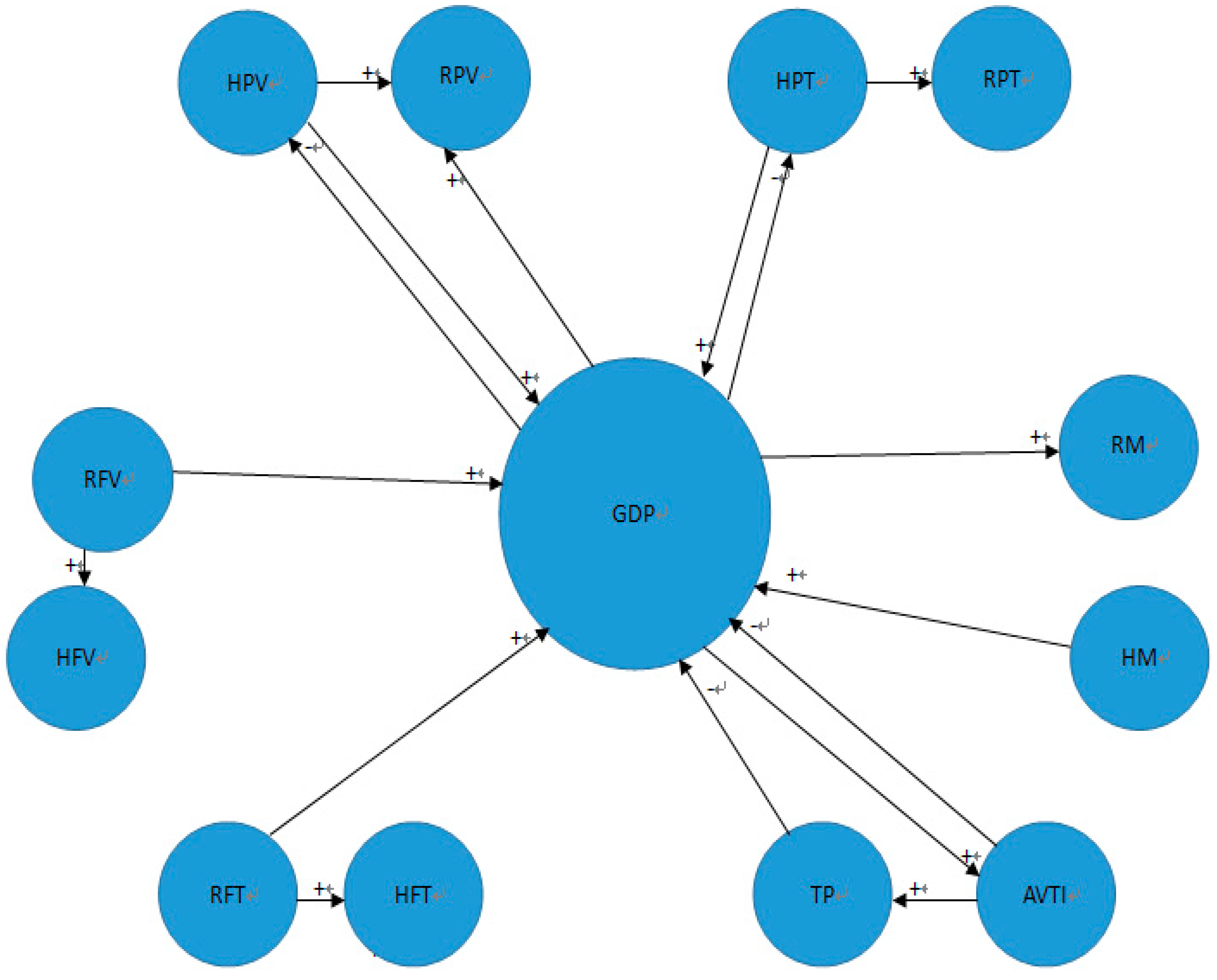
4.2.1. The Relationship between GDP and Land Transportation

To analyze the competitive relationships among different types of land transportation (including highway transportation and railway transportation) and GDP, the parameters in Equation (3) are estimated. The estimation results and R-squares are summarized in panels A to E of

Table 3. Estimation results for land transportation and GDP, 1985~2015.

Panel A: GDP-HPV-RPV
GDP			HPV			RPV
Parameter	Estimates	t-Stat	Parameter	Estimates	t-Stat	Parameter	Estimates	t-Stat
α1	1.23 ***	11.88	α2	1.21 **	2.59	α3	1.41 **	2.62
β11	−3.48 × 10−6 ***	14.82	β21	3.61 × 10−5 ***	−3.08	β31	−1.50 × 10−4 ***	2.89
β12	−0.02 **	2.54	β22	−0.01 ***	8.37	β32	−0.15 *	1.88
β13	1.15	−0.40	β23	0.66	0.20	β33	10.28	1.11
R2	0.98			0.96			0.92
MAPE	0.16			0.12			0.11
Panel B: GDP-HPT-RPT
GDP			HPT			RPT
Parameter	Estimates	t-Stat	Parameter	Estimates	t-Stat	Parameter	Estimates	t-Stat
α1	1.26 ***	11.88	α2	1.09 **	2.29	α3	1.16 **	4.90
β11	−1.13 × 10−5 ***	12.35	β21	1.25 × 10−4 ***	−4.55	β31	−3.23 × 10−5	0.38
β12	−7.19 × 10−4 ***	3.57	β22	−2.28 × 10−3 ***	8.41	β32	−1.02 × 10−3 **	2.61
β13	2.49 × 10−3	−0.99	β23	1.91 × 10−3	0.34	β33	3.60 × 10−3 ***	3.79
R2	0.98			0.91			0.98
MAPE	0.16			0.14			0.07
Panel C: GDP-HFV-RFV
GDP			HFV			RFV
Parameter	Estimates	t-Stat	Parameter	Estimates	t-Stat	Parameter	Estimates	t-Stat
α1	1.29 ***	11.88	α2	1.28 ***	3.45	α3	1.07 ***	3.43
β11	−3.31 × 10−5 ***	12.26	β21	−9.76 × 10−5	1.25	β31	3.48 × 10−5	−1.44
β12	0.08	−1.17	β22	0.22 ***	2.89	β32	−0.05	0.99
β13	−0.16 **	2.76	β23	−0.58 **	2.71	β33	0.23 ***	7.94
R2	0.98			0.98			0.99
MAPE	0.16			0.07			0.06
Panel D: GDP-HFT-RFT
GDP			HFT			RFT
Parameter	Estimates	t-Stat	Parameter	Estimates	t-Stat	Parameter	Estimates	t-Stat
α1	1.21 ***	11.88	α2	1.23 ***	4.42	α3	1.10 ***	8.87
β11	−1.16 × 10−5 ***	6.64	β21	−1.58 × 10−4	1.08	β31	6.05e−07	0.04
β12	2.43 × 10−4	0.13	β22	1.82 × 10−3 **	2.22	β32	1.96 × 10−5	−0.33
β13	−5.17 × 10−5 **	2.66	β23	−4.39 × 10−4 ***	3.35	β33	2.32 × 10−5 ***	17.00
R2	0.98			0.98			0.99
MAPE	0.16			0.10			0.08
Panel E: GDP-HM-RM
GDP			HM			RM
Parameter	Estimates	t-Stat	Parameter	Estimates	t-Stat	Parameter	Estimates	t-Stat
α1	1.23 ***	11.88	α2	1.19 **	2.16	α3	1.35 **	2.50
β11	7.66 × 10−6 ***	14.93	β21	−3.44 × 10−5	−0.91	β31	−8.38 × 10−5 **	2.63
β12	−3.35 × 10−3 **	2.49	β22	1.66 × 10−2 ***	8.67	β32	−1.98 × 10−5	−0.03
β13	0.25	0.71	β23	0.22	1.68	β33	1.77 ***	4.92
R2	0.98			0.99			0.95
MAPE	0.16			0.07			0.06
Panel F: GDP-AVTI-TI
GDP			AVTI			TI
Parameter	Estimates	t-Stat	Parameter	Estimates	t-Stat	Parameter	Estimates	t-Stat
α1	1.22 ***	11.88	α2	1.31 ***	6.56	α3	1.24 ***	3.97
β11	−1.37 × 10−5 ***	11.63	β21	−1.10 × 10−4 ***	3.26	β31	−1.14 × 10−4	0.10
β12	7.83 × 10−4	−1.22	β22	2.93 × 10−3 ***	8.58	β32	6.07 × 10−4	1.44
β13	−1.28 × 10−4	−0.95	β23	−8.96 × 10−5	−1.21	β33	1.34 × 10−3 ***	5.18
R2	0.98			0.95			0.93
MAPE	0.16			0.18			(0.23)
Panel G: GDP-AVTI-TP
GDP			AVTI			TP
Parameter	Estimates	t-Stat	Parameter	Estimates	t-Stat	Parameter	Estimates	t-Stat
α1	1.38 ***	11.88	α2	28.70 ***	6.56	α3	1.05 ***	12.21
β11	−2.58 × 10−5 ***	22.84	β21	−2.65 × 10−3 ***	3.78	β31	2.12 × 10−6	−1.43
β12	6.86 × 10−4 ***	−3.63	β22	3.47 × 10−2 ***	7.37	β32	−8.92 × 10−5 **	2.08
β13	0.87 ***	4.16	β23	138.57	−0.49	β33	0.23 ***	45.08
R2	0.98			0.94			0.99
MAPE	0.16			0.18			0.02
Panel H: GDP-TI-TP
GDP			TI			TP
Parameter	Estimates	t-Stat	Parameter	Estimates	t-Stat	Parameter	Estimates	t-Stat
α1	1.61 ***	11.88	α2	8.44 × 1035 ***	3.97	α3	1.04 ***	12.21
β11	−1.40 × 10−5 ***	10.53	β21	−1.61 × 1032	1.53	β31	2.15 × 10−6	−0.97
β12	9.37 × 10−5	−0.85	β22	1.57 × 1033 ***	5.17	β32	−3.66 × 10−5	1.16
β13	2.25 *	2.04	β23	4.61 × 1036	−1.65	β33	0.10 ***	50.68
R2	0.98			(0.80)			0.99
MAPE	0.16			(0.24)			0.02

Notes: ***, **, and * indicate 1%, 5%, and 10% levels of statistical significance, respectively. Figures in parentheses are MAPEs of ARIMA models.

.

Using Equation (4), the estimated parameters of α_i and β_ij in Equation (3) are transformed into estimated parameters of a_i and b_ij in Equation (1). The sign of β_ij is the same as the sign of b_ij, since (${\mathrm{e}}^{{\mathrm{a}}_{\mathrm{i}}}-1$)/a_i is always positive for a_i > 0, and the sign of a_i is positive if α_i > 1. In each of the Lotka-Volterra models, R-squared is greater than 0.90, except for the added value of transportation industry, where R-squared is 0.80. The MAPE value is 0.23 and 0.24 for the added value of transportation industry and transportation investment, and less than 0.20 for all other analyses. Based on the criteria of Lewis [20], all equations show highly accurate forecasts. The results are summarized in Table 3.

Panel A of Table 3 shows the results for the GDP-HPV-RPV competitive model. Estimated β₁₂, β₂₁, β₃₁, and β₃₂ are statistically significant; other effects are statistically insignificant. The relationship between β₁₂ and β₂₁ is predator-prey; that is, HPV enhances the growth of GDP, but GDP has a significant weakening effect on HPV. The statistically insignificant β₁₃ and β₃₁ indicate a commensalism relationship, where RPV benefits from GDP without either harming or benefiting GDP. The relationship between β₂₃ and β₃₂ is also commensalism. This indicates that RPV benefits from HPV without either harming or benefiting the latter. We can conclude that the interaction between HPV and GDP is significant. This can be explained by the fact that, with the development of the social economy, people have more flexibility in choosing their way to travel (if time is abundant and the place is far away from their residence, they will choose the train, which contributes to the growth of RPV), resulting in a decrease in HPV. Meanwhile, increasing HPV will greatly promote population circulation, and thus indirectly promote consumption, which can increase GDP. Compared with the highway, the railway has its own advantages: high numbers of passengers, a high safety factor, and long transport distance. Xinjiang is geographically distant, which complements the short board of highway passenger transport, so the RPV benefits from HPV are therefore decided by the natural and geographical conditions in Xinjiang.

Panel B of Table 3 shows the results for the GDP-HPT-RPT competitive model. Estimated β₁₂, β₂₁, and β₃₂ are statistically significant; other effects are statistically insignificant. The relationship between β₁₂ and β₂₁ is the same as GDP and HPV. β₁₃ and β₃₁ indicate a neutralism relationship, where the interaction between GDP and RPT is negligible. The relationship between β₂₃ and β₃₂ is commensalism, which means RPT benefits from HPT without either harming or benefiting the latter. In addition to the benefit from HPT, the effect of RPT on GDP is negligible, which proves that, in the short- and medium-term, highway transportation is the main mode of travel for Xinjiang.

Panel C of Table 3 shows the results for the GDP-HFV-RFV competitive model. Estimated β₁₃ and β₂₃ are statistically significant; other effects are statistically insignificant. β₁₂ and β₂₁ have a neutralism relationship, where the interaction between GDP and HFV is negligible. β₁₃ and β₃₁ indicate a commensalism relationship, where GDP benefits from RFV without either harming or benefiting the latter. The relationship between β₂₃ and β₃₂ is also commensalism, where HFV benefits from RFV without either harming or benefiting the latter. Because of the limitation of truck load and the influence of weather, there are shortcomings in HFV, such as high cost and low loading. Moreover, considering the long geographical distance between regions, it is not the mainstream mode of transportation for goods in Xinjiang. Therefore, the impact of HFV on GDP is negligible. Meanwhile, RFV, with the advantages of long-distance transport, large cargo volumes, and lack of weather issues, as well as its low price and high safety factor, has become the first choice for bulk cargo transport in Xinjiang. The circulation of large quantities of goods has promoted import and export trade, which has contributed to the development of the local economy. HFV benefits from RFV because of its flexible mobility, which allows travel to places trains and planes cannot reach, complementing the short board of fixed line railway freight transport. It is apparent that the relationship between HFV and RFV and their relationship with GDP are closely related to the local geographical conditions in Xinjiang.

Panel D of Table 3 shows the results for the GDP-HFT-RFT competitive model. Estimated β₁₃ and β₂₃ are statistically significant; other effects are statistically insignificant. β₁₂ and β₂₁ have a neutralism relationship, where GDP and HFT barely influence each other. β₁₃ and β₃₁ indicate a commensalism relationship, where GDP benefits from RFT without either harming or benefiting the latter. The relationship between β₂₃ and β₃₂ is the same as HFV and RFV. The relationships of the indicators in Panel D are the same as those in Panel C, and the reasons are also consistent.

Panel E of Table 3 shows the results for the GDP-HM-RM competitive model. Estimated β₁₂ and β₃₁ are statistically significant; other effects are statistically insignificant. β₁₂ and β₂₁ have a commensalism relationship, where GDP benefits from HM without either harming or benefiting the latter. β₁₃ and β₃₁ also indicate a commensalism relationship, which shows that RM benefits from GDP without either harming or benefiting GDP. β₂₃ and β₃₂ indicate a neutralism relationship, where HM and RM barely influence each other. The highway can achieve “point-to-point” transportation, is flexible and convenient, and can reach a wide range, so the increase in HM not only promotes population circulation in Xinjiang territory and between the other provinces, but also acts as a supplement to the short board of rail transport of goods. In this way, it plays an important role in promoting the rapid growth of GDP, while the rapid growth of GDP, in turn, can provide reliable financial support for the expansion of Xinjiang’s railway network. However, railways and highways are two separate modes of transportation, and their development models are completely different; therefore, we conclude that though the commensalism between them and GDP is significant, it does not lead to a linear relationship.

4.2.2. The Competitive Relationship among the Economic Indicators of Transportation and Their Relationship with GDP

To analyze the competitive relationships among the economic indicators of transportation and their relationship with GDP, the parameters of Equation (3) are estimated again. The estimation results and R-squared are given in panels F to H of Table 3.

Panel F of Table 3 shows the results for the GDP-AVTI-TI competitive model. Estimated β₂₁ is statistically significant; other effects are statistically insignificant. β₁₂ and β₂₁ indicate a commensalism relationship, where AVTI benefits from GDP without either harming or benefiting the latter. β₁₃ and β₃₁ indicate a neutralism relationship, and β₂₃ and β₃₂ are the same. This indicates that there is barely any interaction between these factors. GDP includes AVTI, which is part of the tertiary industry in GDP. Therefore, GDP will increase accordingly as AVTI increases. The interaction between TI and AVTI is negligible, because the relationship between them is not a simple “input-output” relationship, but is instead very complicated. Studies have shown that several cities in the same region have adopted the same strategy of increasing transportation investment to promote local economic development, but the results differ. Transport investment does not necessarily lead to economic development; only under certain conditions can transportation investment stimulate and promote economic development [24,25].

Panel G of Table 3 presents the results for the GDP-AVTI-TP competitive model. β₃₁ and β₂₃ are statistically insignificant; all other effects are statistically significant. The relationship between β₁₂ and β₂₁ is predator-prey; that is, GDP enhances the growth of AVTI, but GDP is weakened to a certain degree by the latter. β₁₃ and β₃₁ indicate an amensalism relationship, where TP inhibits the growth of GDP, and TP is unaffected by GDP. β₂₃ and β₃₂ indicate a commensalism relationship, where TP benefits from AVTI without either harming or benefiting the latter. Xinjiang is a typical oasis economy region, which means its economic development is determined by its natural resources. The consumption of resources caused by an increasing population places great pressure on the limited resources of the oasis, and this will have a negative impact on its economy’s sustainable development, thus slowing the growth rate of GDP. The increase in AVTI can enable people to travel more conveniently, which greatly increases the circulation of personnel between counties and cities. The contribution of GDP to AVTI has been explained in the discussion of Panel F. Due to the long investment cycle of transportation infrastructure construction and the lag in its economic benefits, transportation investment will have a negative impact on the development of other industries in the short-term, thus affecting the rapid development of the overall national economy.

Panel H of Table 3 shows the results for the GDP-TI-TP competitive model. Estimated β₁₃ is statistically significant; other effects are statistically insignificant. β₁₂ and β₂₁ indicate a neutralism relationship, and β₂₃ and β₃₂ are the same. This shows the interaction between these factors is negligible. TI and TP are of different statistical categories, so there is no linear relationship.

In Figure 2, we summarize all the statistically significant results from the LV-COMSUD models. In summary, the interactions among land transportation and GDP derived from the LV-COMSUD models include: (1) Predator-prey, such as where HPV and HPT enhance the growth of GDP, but GDP has a significant weakening effect on them. (2) Commensalism, where GDP benefits from HM without either harming or benefiting the latter. (3) Neutralism, where TI, GDP, AVTI, and TP barely influence each other. (4) Amensalism, as seen when TP inhibits the growth of GDP, and TP is unaffected by GDP.

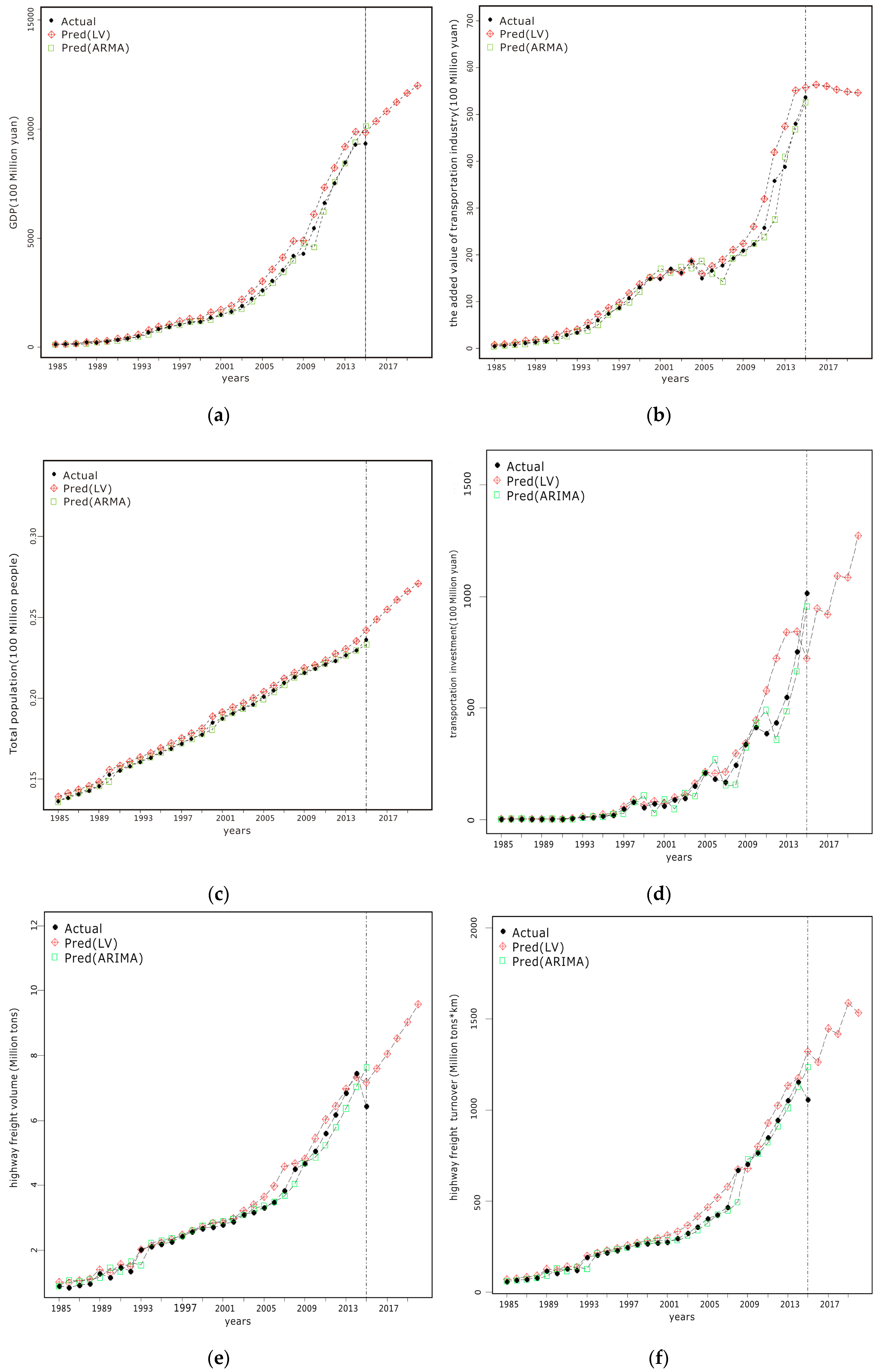
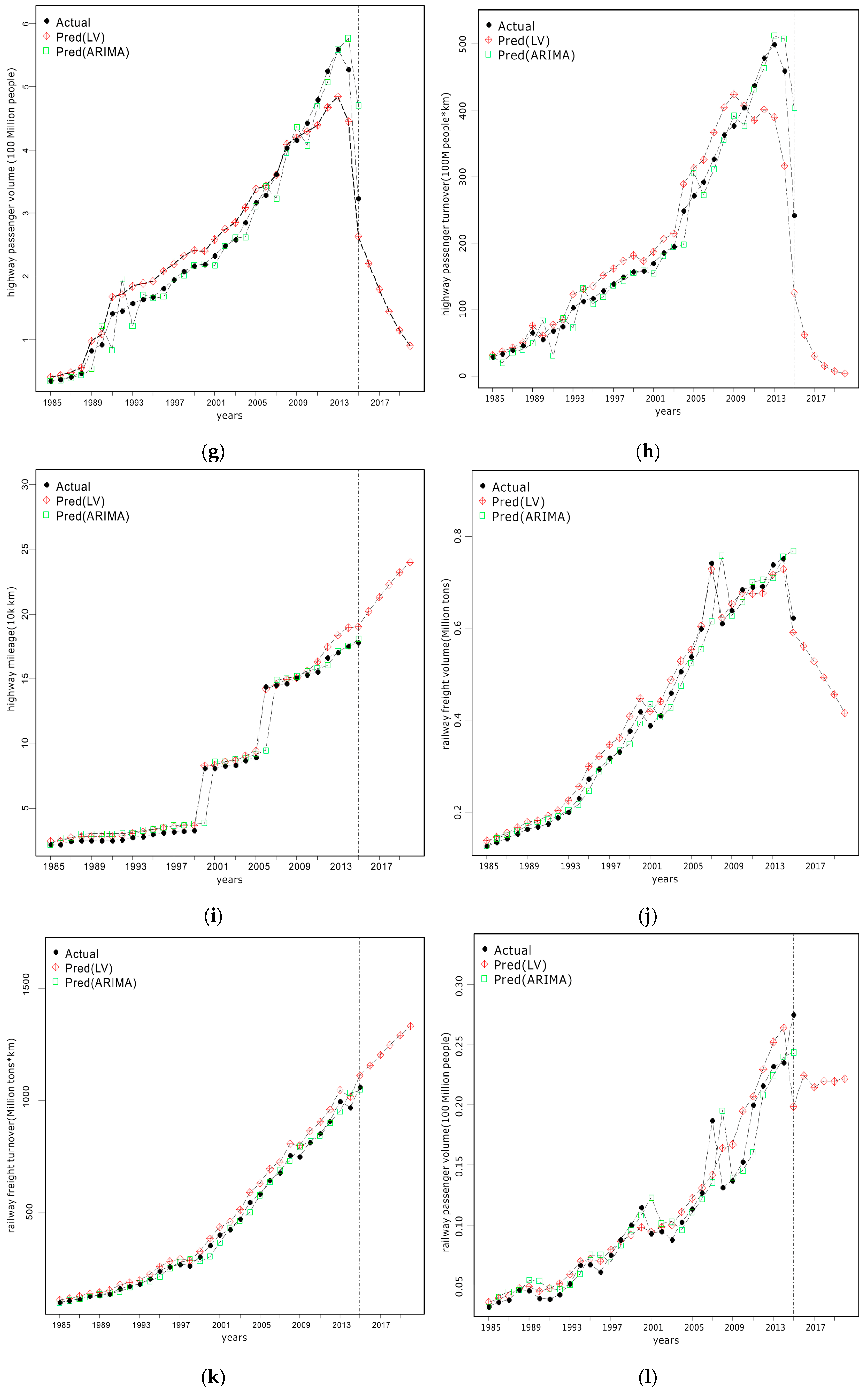
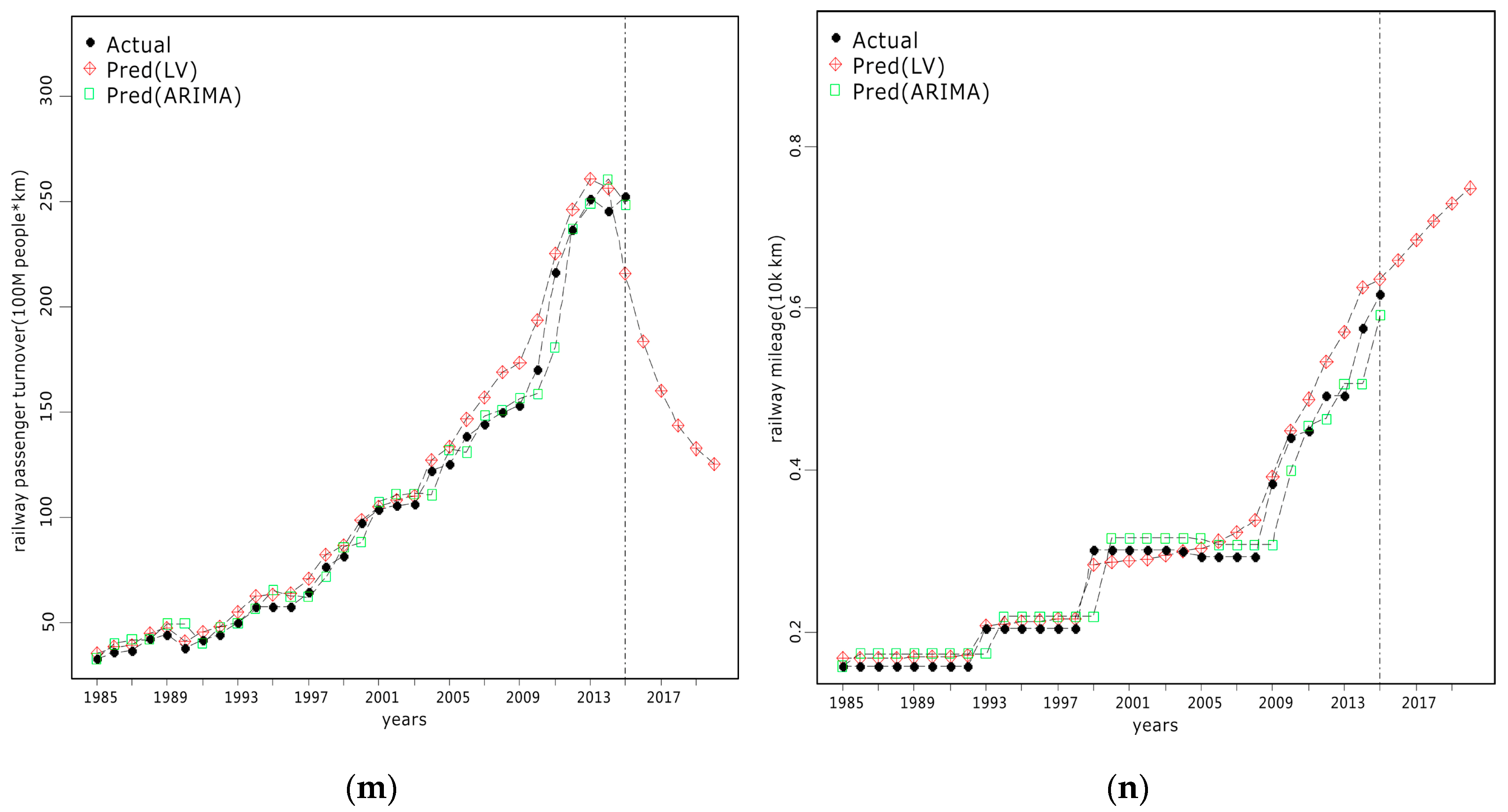
4.3. Forecasting Land Transportation, the Economic Indicators of Transportation and GDP

Due to the data itself, there is a large error in the prediction of the ARIMA model. Therefore, when predicting future data, only the prediction results of the LV model are used. The multivariate LV-COMSUD model is estimated using actual Xinjiang data from 1985 to 2015 to predict the variables of land transportation and GDP. The MAPE statistics, computed as in Equation (1), are used to assess these models’ in-sample forecasting ability. The model has good predictive ability, as reflected in the MAPEs of less than 0.2 in

Table 4. Forecast of parameters, 2016–2020.

	GDP	HPV	RPV	HFV	RFV	HM	RM	AVTI	TI	TP
2016	10,336.9	2.21	0.22	7.59	0.56	20.18	0.66	562.97	949.1	0.25
2017	10,807.07	1.79	0.21	8.04	0.53	21.28	0.68	559.81	921.9	0.26
2018	11,240.44	1.44	0.22	8.52	0.49	22.28	0.71	553.25	1093.0	0.26
2019	11,634.49	1.14	0.22	9.04	0.46	23.19	0.73	547.84	1086.1	0.27
2020	11,988.91	0.90	0.22	9.59	0.42	24.00	0.75	546.63	1274.4	0.27
CAGR-lv (%)	5.15	−19.40	2.24	5.97	−6.75	4.76	3.33	0.39	4.61	2.81
RE-LV (2016)	0.07	−0.24	−0.3	0.17	−0.19	0.11	−0.07	−0.01	0.14	0.04
RE-LV(2020)	−0.08	−0.9	−0.62	−0.24	−0.76	0.26	−0.25	−0.15	−0.03	0.03

Note: CAGR-LV (%) is annual growth rate in 5-year for the average forecasting result of LV models. RE-LV (2016) and RE-LV (2020) are the relative errors of the predicted values and the actual target values in 2016 and 2020, respectively.

.

For the out-of-sample forecast of land transportation and GDP in Xinjiang from 2016 to 2020, the results using LV-COMSUD models are displayed in Figure 1 and Table 4. Table 4 also shows the 5-year CAGRs between 2016 and 2020 for variables in the LV-COMSUD models. According to Table 3, we can conclude that HPV and RFV will decline in the next five years (HPV especially decreases by 19.4%), while the others will maintain a slow upward trend. This is because the policy of the ‘Thirteenth Five-Year Plan’ in Xinjiang promotes the coordinated development of various modes of transportation, which will make transportation modes more flexible.

Because the four indicators, GDP, AVTI, TP, and TI, were included in two or more forecasts, the final results are selected based on the MAPE values in each group and the degree of closeness to the actual value. Based on the criteria in Lewis [20], the prediction results shown in Panels G, E, and H are reasonable. RE-LV (2016) and RE-LV (2020) are the relative errors of the predicted values and the actual target values in 2016 and 2020, respectively.

5. Conclusions and Discussion

This study employs the LV-COMSUD model to capture the competitive interactions among GDP and land transportation, as well as the competitive interactions among different types of land transportation (highway and railway). Understanding the different types of interactions among GDP and land transportation (mutualism, commensalism, predator-prey, amensalism, or neutralism) not only facilitates policy development to achieve a balance in the relationship between economy and transportation, but can also provide technical support and a scientific basis for the advancement of transportation development planning.

Our findings have important practical implications. In particular, the findings suggest the following. (1) HM, highway passenger transportation, and railway freight transportation have a large positive impact on promoting the national economy of Xinjiang, which will weaken the development of highway passenger transportation and promote the development of railway passenger transportation, railway mileage, and AVTI. (2) Highway passenger transportation promotes the development of railway passenger transportation, while rail freight transportation has played an important role in promoting highway freight transportation in Xinjiang. (3) The increase of AVTI is conducive to the growth of TP, but both have a certain negative impact on the national economy in the short-term. (4) There is no significant relationship between TI and the national economy. The fourth conclusion is consistent with some of the existing research. The quantitative correlation between transportation construction investment and GDP growth has been analyzed, but the studies were unable to reveal the direct effect of regional leading industry through transportation construction investment in selected cities [26,27,28,29]. In addition, transportation infrastructure construction has different impacts on regional economic development, which are caused by changes in the socio-economic environments studied. This shows that technological factors (especially advances in information technology leading to the flow of intangible elements of production, such as increased information and funds) and increasing efficiency became more and more essential to regional economic development, which may lead to an obvious result that additional transportation investment in the original socio-economic environment can stimulate and promote economic development. Meanwhile, with the changes in environment, it is possible that additional transportation investment will become a serious burden to economic development; a high-quality infrastructure is not a necessary condition for emerging areas in recession or economic growth [30].

Xinjiang has unique natural and geographical conditions, as well as a special strategic position, and the reality is that there may still be a giant gap between rich and poor people [31]; the level of economic development in Xinjiang is in a backward position in the country. The primary task of economic development is poverty alleviation and the maintenance of social stability; therefore, many infrastructure investments have focused on this target. On the other hand, transportation infrastructure construction requires a huge amount of investment over the long-term, but its economic benefits have a certain lag. Thus, there is no significant relationship between this indicator and the others in the short-term.

As the current research illustrates, Lotka-Volterra equations provide a simple model to capture the main characteristics of the dynamic competition between GDP and land transportation in Xinjiang. In reality, however, many additional factors affect the economy and transportation, so it cannot capture all the possible relationships. Future research should apply the LV-COMSUD framework to develop more parameters and comparisons in different research areas; the results should be helpful in transportation planning.

References

1. Yang, Z.S.; Fan, J.M. Transportation and Economic Development. Econ. Issues 1995, 8, 42–43. [Google Scholar]
2. Lu, D.D. The Theory and Practice of China’s Regional Development, 1st ed.; Science Press: Beijing, China, 2003; pp. 221–222. ISBN 9787030112040. [Google Scholar]
3. Edward, J.T.; Howard, L.G. Geography of Transportation, 2nd ed.; Prentice Hall: Upper Saddle River, NJ, USA, 1996; pp. 38–43. ISBN 0133685721. [Google Scholar]
4. Liu, J.Q.; He, J.H. An Empirical Study on the Development of Transportation Industry and National Economy. J. Transp. Syst. Eng. 2002, 2, 82–86. [Google Scholar]
5. Garcia, M.T.; McGuire, T.J.; Porter, R.H. The effect of public capital in state level production functions reconsidered. Rev. Econ. Stat. 1996, 78, 177–180. [Google Scholar] [CrossRef]
6. Holtz, E.D.; Schwarz, A.E. Spatial productivity spillovers from public infrastructure: Evidence from state highways. Int. Tax Public Financ. 1995, 2, 459–468. [Google Scholar] [CrossRef]
7. Mehmet, A.B.; Müge, K.; Hakan, Y. Granger-causality between transportation and GDP: A panel data approach. Transp. Res. Part A 2014, 63, 43–55. [Google Scholar]
8. Michael, I.; David, L. Mutual causality in road network growth and economic development. Transp. Policy 2016, 45, 209–217. [Google Scholar]
9. Kveiborg, O.; Fosgerau, M. Decomposing the decoupling of Danish road freight traffic growth and economic growth. Transp. Policy 2007, 14, 39–48. [Google Scholar] [CrossRef]
10. Li, Y.C.; Zhao, L.; Suo, J.J. Comprehensive Assessment on Sustainable Development of Highway Transportation Capacity Based on Entropy Weight and TOPSIS. Sustainability 2014, 6, 4685–4693. [Google Scholar] [CrossRef]
11. Feng, H. An Analysis of the Contribution of Highway Traffic to Xinjiang’s National Economic Growth. Master’s Thesis, Shanghai Maritime University, Shanghai, China, 2005. [Google Scholar]
12. Xu, C.F. Research of the Relationship between Highway Traffic and the Development of Economy and Society in Xinjiang Production and Construction Corps. Ph.D. Thesis, Wuhan University of Technology, Wuhan, China, 2011. [Google Scholar]
13. Zhu, Y.N. Research on the relationship between regional transport and regional economic in southern Xinjiang. Master’s Thesis, Beijing Jiaotong University, Beijing, China, 2011. [Google Scholar]
14. Zhang, L.; Zhang, X.L.; Du, H.R.; Ni, T.Q. The Different Impact of Passenger Traffic Way son the Different Economic Growth in Xinjiang Region. J. Chongqing Norm. Univ. (Nat. Sci.) 2016, 33, 211–216. [Google Scholar]
15. Lotka, A.J. Elements of Physical Biology, 1st ed.; Williams & Wilkins Co.: Baltimore, MA, USA, 1925. [Google Scholar]
16. Volterra, V. Leconssur la Theoriemathematique de la Lutte Pour la vie; Gauthier-Villars: Paris, France, 1931. [Google Scholar]
17. Wang, X.W. Analysis on application effect of Xinjiang Highway Transportation 11th Five-year Plan. Master’s Thesis, Changan University, Xi’an, China, 2010. [Google Scholar]
18. Development Plan of “13th Five—Year Plan” of Transportation in Xinjiang Uygur Autonomous Region. Available online: http://www.xjjt.gov.cn/article/2015-11-23/art84330.html (accessed on 3 July 2015).
19. Box, G.E.P.; Jenkins, G.M. Time Series Analysis: Forecasting and Control; Holden-Day: San Francisco, CA, USA, 1976. [Google Scholar]
20. Lewis, C.D. Industrial and Business Forecasting Methods: A Practical Guide to Exponential Smoothing and Curve Fitting; Butter-Worth-Heinemann: London, UK, 1982. [Google Scholar]
21. Girifalco, L.A. Dynamics of Technological Change, 1st ed.; Van Nostrand Reinhold: New York, NY, USA, 1991; ISBN 978-1-4684-6511-2. [Google Scholar]
22. Liu, P.Z.; Gopalsamy, K. On a model of competition in periodic environments. Appl. Math. Comput. 1997, 82, 207–238. [Google Scholar] [CrossRef]
23. Pistorius, C.W.I.; Utterback, J.M. A Lotka-Volterra Model for Multi-Mode Technological Interaction: Modelling Competition, Symbiosis and Predator Prey Modes; Working Papers; Massachusetts Institute of Technology (MIT), Sloan School of Management: Cambridge, MA, USA, 1996; pp. 3929–3996. [Google Scholar]
24. Hart, T. Transport Investment and Disadvantage Regions: UK and European policies since the 1950s. Urban Stud. 1993, 30, 417–435. [Google Scholar] [CrossRef]
25. Banister, D. Transport Planning in the UK, USA and Europe, 1st ed.; E & FN Spon: London, UK, 1994; ISBN 0-419-18930-0. [Google Scholar]
26. Aschauer, A.D. Is Public Expenditure Productive? J. Monetary Econ. 1988, 23, 177–200. [Google Scholar] [CrossRef]
27. Munnell, A.H. Why Has Productivity Growth Declined? Productivity and Public Investment. N. Engl. Econ. J. Rev. 1990, 30, 3–22. [Google Scholar]
28. Durkin, J.T., Jr.; Wassmer, R.W. Public Infrastructure Spending and Private Generation in Large US Cities; Working Paper; Lincoln Institute of Land Policy: Cambridge, MA, USA, 1994. [Google Scholar]
29. Holtz-Eakin, D.; Schwartz, A.E. Infrastructure in a Structural Model of Economic Growth. Reg. Sci. Urban Econ. 1994, 25, 131–151. [Google Scholar] [CrossRef]
30. Botham, R. Regional Development Effects of Road Investment. Transp. Plan. Technol. 1980, 6, 97–108. [Google Scholar] [CrossRef]
31. Liu, X.T.; Chen, W.J. Dynamics of spatial pattern of county's economics during 2004–2013 in Xinjiang, China. J. Desert Res. 2015, 35, 1089–1095. [Google Scholar]
Figure 1. Actual data and model output (Actual: Actual data of each variable from 1985 to 2015; Pred (LV): Lotka-Volterra model prediction; Pred (ARIMA): Autoregressive integrated moving average results). (a) the variation tendency of GDP; (b) the variation tendency of AVTI; (c) the variation tendency of TP; (d) the variation tendency of TI; (e) the variation tendency of HFV; (f) the variation tendency of HFT; (g) the variation tendency of HPV; (h) the variation tendency of HPT; (i) the variation tendency of HM; (j) the variation tendency of RFV; (k) the variation tendency of RFT; (l) the variation tendency of RPV; (m) the variation tendency of RPT; (n) the variation tendency of RM). Notes: Meanings of abbreviations in Figure 1 are all refer to Table 1.
Sustainability 10 00135 g001aSustainability 10 00135 g001bSustainability 10 00135 g001c
Figure 2. Dynamic competitive relationships among land transportation and GDP.
Sustainability 10 00135 g002