An Adaptive Weight Collaborative Driving Strategy Based on Stackelberg Game Theory

Abstract

In response to the problem of cooperative steering control between drivers and intelligent driving systems, a master–slave Game-Based human–machine cooperative steering control framework with adaptive weight fuzzy decision-making is constructed. Firstly, within this framework, a dynamic weight approach is established. This approach takes into account the driver’s state, traffic environment risks, and the vehicle’s global control deviation to adjust the driving weights between humans and machines. Secondly, the human–machine cooperative relationship with unconscious competition is characterized as a master–slave game interaction. The cooperative steering control under the master–slave game scenario is then transformed into an optimization problem of model predictive control. Through theoretical derivation, the optimal control strategies for both parties at equilibrium in the human–machine master–slave game are obtained. Coordination of the manipulation actions of the driver and the intelligent driving system is achieved by balancing the master–slave game. Finally, different types of drivers are simulated by varying the parameters of the driver models. The effectiveness of the proposed driving weight allocation scheme was validated on the constructed simulation test platform. The results indicate that the human–machine collaborative control strategy can effectively mitigate conflicts between humans and machines. By giving due consideration to the driver’s operational intentions, this strategy reduces the driver’s workload. Under high-risk scenarios, while ensuring driving safety and providing the driver with a satisfactory experience, this strategy significantly enhances the stability of vehicle motion.

1. Introduction

The emergence of autonomous driving has relieved the burden on drivers and even mitigated the risk of accidents [1,2]. Nevertheless, achieving fully autonomous driving (Level 5) remains a long-term goal. Given the intricate traffic environment and legal complexities, vehicle control still cannot be completely decoupled from drivers [3]. Thus, despite rapid progress in autonomous driving technology, the human–machine co-driving stage will persist for some time into the future. The core technology in human–machine co-driving is human–machine collaborative driving technology. Here, driving authority is not monopolized by one party but is jointly determined through collaboration between the vehicle and the driver, integrating their respective decisions [4].

In the context of human–machine collaborative driving, the real-time driving authority allocation strategy dictates the vehicle’s driving trajectory. For example, the researchers Fang et al. [5] utilized the tracking error in vehicle state data to quantify the driver’s path-following ability under diverse driving conditions and accordingly determined the driving authority allocation. As the driver’s ability improved, the driver’s driving weight increased. The researchers Xu et al. [6] constructed a multi-factor-driven weight allocation module considering human–machine characteristics and collaborative performance. Taking into account the potential field of environmental risks and the human–machine conflict coefficient, the researchers Xie et al. [7] designed an adaptive weight allocation method to allocate weights between the driver and the automated system. The researchers Zhao et al. [8] adopted Gaussian process regression techniques to evaluate driving risks. The driving risks were evaluated from multiple dimensions, including vehicle speed, the front wheel’s steering angle, vehicle stability, and human–machine conflicts. Based on the evaluation results, the driving authority between humans and machines was dynamically allocated. Additionally, investigations have approached the allocation of driving authority from the perspectives of the vehicle or the traffic environment. For instance, Liu Jun et al. [9] established a risk potential field and adjusted the driving weights in accordance with the prevailing driving risk. When the driving risk was elevated, the vehicle’s driving weight was augmented. The researchers Dai et al. [10] employed bargaining games and proposed a utility function for a collaborative driving system. The optimal driving weight allocation scheme was derived by solving the system’s maximum utility function.

In human–machine collaborative driving, both the driver and the autonomous driving system are capable of independently fulfilling driving tasks and are thus regarded as two autonomous agents. Game theory has proven to be an effective approach to addressing the collaborative control issues between two agents. The researchers Zhou et al. [11] established a methodology that took into account the uncertainties in the driving behaviors of surrounding autonomous vehicles. This methodology is founded on game theory and distributed model predictive control. Eventually, it was integrated into a multi-objective constrained problem. In the course of human–machine shared steering control, the researchers Feng et al. [12] incorporated cooperative game theory to determine the level of interactive control. Moreover, they put forward a robust H∞ compensation control approach to enhancing the anti-interference capabilities of the system, thus guaranteeing the stability of the vehicle. The researchers Lu et al. [13] integrated a designed game entry mechanism with a re-planned game sequence under different intersection conditions and constructed a variable game model to address the driving conflicts of autonomous vehicles at unsignalized intersections. The researchers Liu et al. [14,15] put forward a three-level Game-Based decision-making framework. Ultimately, a neural network was utilized to learn the decision-making outcomes derived from the game approach. This method enables autonomous vehicles to respond in a timely manner when interacting with drivers featuring diverse driving styles in the surroundings. The researchers Li et al. [16] employed game theory to address the conflict between tracking accuracy and driving stability in the context of lane-changing for driverless vehicles. The researchers Wang et al. [17] introduced cooperative game theory to model the steering interaction of dual controllers. An adaptive weight adjustment strategy based on the predicted output deviation was designed to achieve collaborative optimization of dual steering control. Even when partial steering fails, fault-tolerant steering control is also achieved through cooperative game theory.

This study focuses on a description of the relationship between the driver and the co-driving controller, as well as the issue of driving authority allocation. The aim is to alleviate the driver’s operational burden while ensuring vehicle driving safety. A master–slave game model for human–machine interaction behavior is constructed. Based on this, an adaptive weight decision-making model grounded in fuzzy control rules is proposed. This model modifies the conditions of the human–machine game equilibrium to accomplish the path-tracking task. The experimental results indicate that the method put forward in this paper can effectively reduce the driver’s burden, enhance the stability of vehicle motion, and assist drivers in various states to fulfill driving tasks.

2. Modeling of the Vehicle Dynamics and Human–Machine Steering Controllers

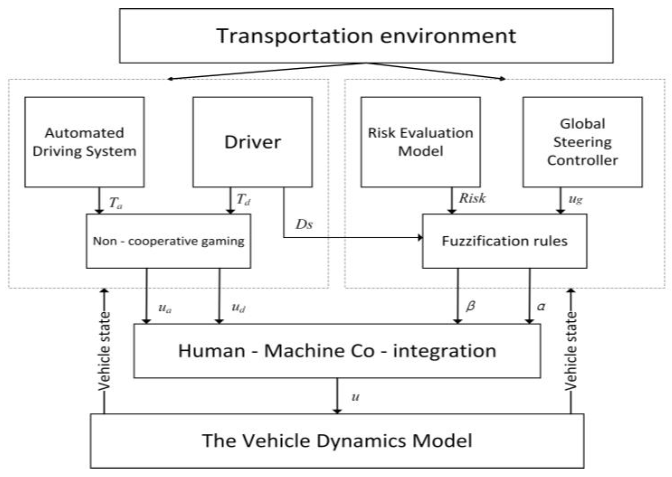
2.1. The Control Architecture

The co-driving control system diverges from traditional driving assistance systems. As an independent virtual co-driver, the co-driving controller possesses a certain level of autonomy. It can make autonomous decisions based on environmental perception information to provide assistance to the driver. The human–machine control actions are accomplished through a hybrid approach in accordance with the driving authority allocation, thereby realizing human–machine collaborative steering control. The autonomous driving system constructs a human–machine interaction model by obtaining its own expectation ($T_a$) and the driver’s expectation ($T_d$). It predicts the driver’s control action ($u_d$) and formulates its own optimal response ($u_a$). The global steering controller computes the global optimal control variable ($u_g$). The fuzzy logic controller takes the driver’s state ($Ds$); the degree of the deviation between the actual vehicle’s control input and the global optimal control; and the traffic environment risk ($Risk$) as inputs and outputs the driving weights ($\alpha$,$\beta$), both human and machine, in real time. The human–machine integration module determines the linear combination of the control variables of the human and the machine according to their weights and uses this as the final control variable ($u$) to command the vehicle to execute steering maneuvers. Non-cooperative game theory is employed to establish the human–machine interaction model, which is characterized as a Stackelberg game. The human–machine conflict issue is addressed by deriving the optimal control strategies for both the human and the machine. Subsequently, an adaptive weight decision model based on fuzzy rules is utilized to dynamically adjust the driving authorities of the human and the machine. This adjustment modifies the equilibrium conditions of the human–machine game, ensuring the safe operation of the vehicle. The overall framework is presented in Figure 1.

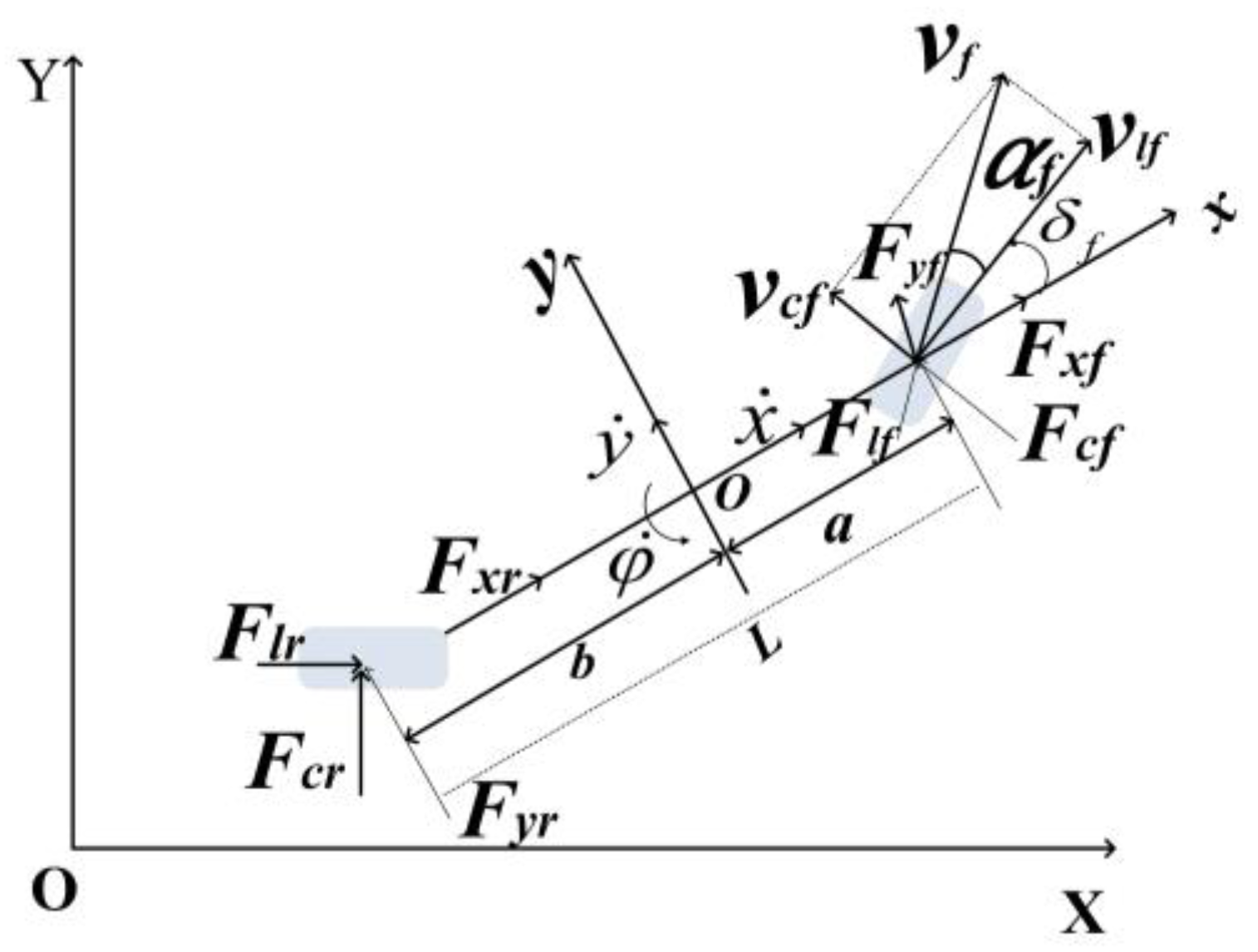
2.2. Modeling of the Vehicle Dynamics

In order to design the human–machine collaborative control model and reduce the computational complexity of the control algorithm, a three-degree-of-freedom single-track vehicle dynamics model [18], as depicted in Figure 2, is established. This is achieved by disregarding factors such as changes in the longitudinal velocity, the differences between the front and rear wheels, longitudinal and lateral aerodynamics, and the impact of the suspension system. XOY is the global coordinate system, while xoy is the vehicle-fixed coordinate system. $F_{lf}$ and $F_{lr}$ represent the longitudinal resultant forces of the front and rear tires, respectively; $F_{cf}$ and $F_{cr}$ represent the net lateral forces of the front and rear tires, respectively; $v_{cf}$ is the lateral velocity of the front wheel; $v_{lf}$ is the longitudinal velocity of the front wheel; ${\delta }_f$ and ${\delta }_r$ are the steering angles of the front and rear wheels of the vehicle, respectively; $a$ and $b$ are the distances from the vehicle’s center of mass to the front and rear axles, respectively; $v_f$ is the velocity of the front axle’s center; $\dot{\phi }$ is the yaw rate; $a_f$ is the slip angle of the front wheel; $m$ is the mass of the vehicle; $I_z$ is the moment of inertia; $s$ is the slip ratio; $C_l$ is the longitudinal stiffness of the tire; and $C_c$ is the lateral stiffness of the tire.

The transformation relationship between the global coordinate system and the vehicle-fixed coordinate system is

$$\left\{\begin{array}{c}\dot{Y}=\dot{x}\sin \phi +\dot{y}\cos \phi \\ \dot{X}=\dot{x}\cos \phi -\dot{y}\sin \phi \end{array}\right.$$

(1)

In accordance with Newton’s second law, force-equilibrium equations are established along the x-axis and y-axis and about the z-axis, respectively:

$$\left\{\begin{array}{l}m\ddot{x}=m\dot{y}\dot{\phi }+2F_{xf}+2F_{xr}\hfill \\ m\ddot{y}=-m\dot{x}\dot{\phi }+2F_{yf}+2F_{yr}\hfill \\ I_z\ddot{\phi }=2a{F}_{yf}-2b{F}_{yr}\hfill \end{array}\right.$$

(2)

The relationships between the lateral force, the longitudinal force, and the resultant force of the tires in the x-direction and the y-direction are as follows:

$$\left\{\begin{array}{c}{F}_{xf}=F_{lf}\cos {\delta }_f-F_{cf}\sin {\delta }_f\\ F_{xr}=F_{lr}\cos {\delta }_r-F_{cr}\sin {\delta }_r\\ F_{yf}=F_{lf}\sin {\delta }_f+F_{cf}\cos {\delta }_f\\ F_{yr}=F_{lr}\sin {\delta }_r+F_{cr}\cos {\delta }_r\end{array}\right.$$

(3)

In order to simplify the model, the assumption of a low angular velocity is employed, and an approximate relationship can be obtained:

$$\left\{\begin{array}{c}\sin \delta \approx \delta \\ \cos \delta \approx 1\\ \tan \delta \approx \delta \end{array}\right.$$

(4)

Then, Equation (4) can be simplified into

$$\left\{\begin{array}{l}{F}_{xf}=F_{lf}-F_{cf}{\delta }_f\hfill \\ F_{xr}=F_{lr}\hfill \\ F_{yf}=F_{lf}{\delta }_f+F_{cf}\hfill \\ F_{yr}=F_{cr}\hfill \end{array}\right.$$

(5)

To calculate the longitudinal force $F_l$ and the lateral force $F_c$ of the tire, the model is simplified further, and the Pacejka tire model [18] is adopted. When the lateral acceleration $a_y$ ≤ 0.4 g and the tire slip angle $\alpha$ ≤ 5°, according to the magic formula, it is known that

$$\left\{\begin{array}{c}{F}_l=C_{l}s\\ F_c=C_c\alpha \end{array}\right.$$

(6)

In order to calculate the tire camber angle, by analyzing the relationship shown in the figure, we obtain

$$\alpha =\arctan {\displaystyle \frac{v_c}{v_l}}$$

(7)

$$\left\{\begin{array}{c}{v}_l=v_y\sin \delta +v_x\cos \delta \\ v_c=v_y\cos \delta -v_x\sin {\delta }_c\end{array}\right.$$

(8)

$$\left\{\begin{array}{l}{v}_{yf}=\dot{y}+a\dot{\phi }\hfill \\ v_{yr}=\dot{y}-b\dot{\phi }\hfill \\ v_{xf}=\dot{x}\hfill \\ v_{xr}=\dot{x}\hfill \end{array}\right.$$

(9)

Under the premise of an assumed low angular velocity, by jointly considering Equation (7) through to Equation (9), the following result is obtained:

$${\alpha }_f={\displaystyle \frac{\dot{y}+a\dot{\phi }}{\dot{x}}}-{\delta }_f$$

(10)

Regarding the rear wheel’s camber angle, when considering a front wheel drive scenario with ${\delta }_r$ = 0, it follows that

$${\alpha }_r={\displaystyle \frac{\dot{y}-b\dot{\phi }}{\dot{x}}}$$

(11)

By substituting Equations (10) and (11) into Equation (6), the lateral forces and the longitudinal forces of the front and rear wheels are derived as follows:

$$\left\{\begin{array}{l}{F}_{cf}=C_{cf}\left({\displaystyle \frac{\dot{y}+a\dot{\phi }}{\dot{x}}}-{\delta }_f\right)\\ F_{cr}=C_{cr}\left({\displaystyle \frac{\dot{y}-b\dot{\phi }}{\dot{x}}}\right)\end{array}\right.$$

(12)

$$\left\{\begin{array}{c}{F}_{lf}=C_{lf}{s}_f\\ F_{lr}=C_{lr}{s}_r\end{array}\right.$$

(13)

When Equations (12) and (13) are substituted into Equation (5), we obtain

$$\left\{\begin{array}{l}{F}_{xf}=C_{lf}{s}_f-C_{cf}({\displaystyle \frac{\dot{y}+a\dot{\phi }}{\dot{x}}}-{\delta }_f){\delta }_f\\ F_{xr}=C_{lr}{s}_r\\ F_{yf}=C_{lf}{s}_f{\delta }_f+C_{cf}({\displaystyle \frac{\dot{y}+a\dot{\phi }}{\dot{x}}}-{\delta }_f)\\ F_{yr}=C_{cr}({\displaystyle \frac{\dot{y}-b\dot{\phi }}{\dot{x}}})\end{array}\right.$$

(14)

Upon substituting the above equation into the force equilibrium Equation (2), simplified vehicle dynamics equations can be derived:

$$\left\{\begin{array}{l}m\ddot{x}=m\dot{y}\dot{\phi }+2[C_{lf}{s}_f+C_{cf}({\delta }_f-{\displaystyle \frac{\dot{y}+a\dot{\phi }}{\dot{x}}}{\delta }_f){\delta }_f+C_{lr}{s}_r]\\ m\ddot{y}=-m\dot{x}\dot{\phi }+2[C_{lf}{s}_f{\delta }_f+C_{cf}({\displaystyle \frac{\dot{y}+a\dot{\phi }}{\dot{x}}}-{\delta }_f)+C_{cr}({\displaystyle \frac{\dot{y}-b\dot{\phi }}{\dot{x}}})]\\ I_z\ddot{\phi }=2[a{C}_{lf}{s}_f{\delta }_f+C_{cf}({\displaystyle \frac{\dot{y}+a\dot{\phi }}{\dot{x}}}-{\delta }_f)-b{C}_{cr}({\displaystyle \frac{\dot{y}-b\dot{\phi }}{\dot{x}}})]\\ \dot{Y}=\dot{x}\sin \phi +\dot{y}\cos \phi \\ \dot{X}=\dot{x}\cos \phi -\dot{y}\sin \phi \end{array}\right.$$

(15)

The position, velocity, yaw angle, and other information for the vehicle are chosen as the vehicle state variables. These are denoted as $\zeta ={[\begin{array}{c}\dot{y},\dot{x},\phi ,\dot{\phi },Y,X\end{array}]}^{\mathrm{T}}$; when the control variable is chosen as $u=\left[{\delta }_f\right]$ and the output variable is likewise chosen as $\eta ={\left[\phi ,Y\right]}^T$, the equation for the nonlinear dynamics of the vehicle can be formulated as

$$\dot{\zeta }=f\left(\zeta ,u\right)$$

(16)

First, the forward Euler method is employed to discretize the nonlinear model. Given that the sampling time is $T$, we have

$$\dot{\zeta }(k)={\displaystyle \frac{\zeta (k+1)-\zeta (k)}{T}}$$

(17)

By simultaneously considering Equations (16) and (17), we arrive at

$$\zeta (k+1)=\zeta (k)+Tf[\zeta (k),u(k)]$$

(18)

Subsequently, by applying the state-trajectory method to linearizing the system state Equation (18), we obtain

$$\zeta (k+1)-{\widehat{\zeta }}_0(k+1)=A_{k,0}[\zeta (k)-{\widehat{\zeta }}_0(k)]+B_{k,0}[u(k)-u_0(k)]$$

(19)

The equation presented above represents the linear model derived at the operating point $\left({\zeta }_0,u_0\right)$. This model can be extended further to an arbitrary point $\left({\zeta }_t,u_t\right)$. Consequently, a discrete linearized vehicle system model can be achieved.

$$\left\{\begin{array}{l}\zeta (k+1)=A\zeta (k)+Bu(k)+d(k)\\ \eta =C\zeta \end{array}\right.$$

(20)

In the formula, $d(k)={\widehat{\zeta }}_t(k+1)-A_{k,t}{\widehat{\zeta }}_t(k)-B_{k,t}{u}_t(k)$, $A=A_{k,t}$, $B=B_{k,t}$, and $C=\left[\begin{array}{cccccc}0& 0& 1& 0& 0& 0\\ 0& 0& 0& 0& 1& 0\end{array}\right]$.

2.3. The Driver Model

Taking into account the intricate circumstances of repetitive experiments involving real-life drivers, in order to analyze the experimental results with greater precision, this study employs the optimal preview lateral acceleration driver model [19]. The steering wheel’s angle in the driver output of this model is presented in Equation (21). This model simultaneously considers the driver’s reaction latency and the correction mechanism. By simulating the driver’s actions of making judgments and implementing rolling adjustments based on the current vehicle’s driving state and comparing the deviation between the future trajectory for a previewed timepoint and the target trajectory, it can effectively mirror the performance of human drivers during driving tasks.

$$\left\{\begin{array}{l}{\delta }_{sw}^{\ast }=\ddot{y}{(t)}^{\ast }·C_1·C_2\\ \ddot{y}(t)={\displaystyle \frac{2}{T_p^2}}[y(t+T_p)-y(t)-T_p\dot{y}(t)]\\ C_1={\displaystyle \frac{1+T_c}{G_{ay}}}\\ C_2={\displaystyle \frac{\exp (-T_{d}s)}{1+T_{h}s}}\end{array}\right.$$

(21)

Specifically, $\ddot{y}(t)$ represents the ideal lateral acceleration derived from the optimization objective of minimizing the tracking error; $C_1$ denotes the correction element; $G_{ay}$ stands for the steady-state gain function of the lateral acceleration; $C_2$ refers to the reaction lag component; $T_p$ is the preview time; $T_h$ is the delay time for muscle action; and $T_d$ is the delay time for a neural reaction.

Real drivers’ states can be influenced by factors such as emotions, the environment, their physical condition, and even alcohol consumption. This has a direct impact on driving safety. The driving state of drivers can be classified or quantified by means of a driver state detection system, operational signals, and vehicle status information. Regarding the driver model, different parameters can be utilized to characterize the driver’s state. In the relevant literature, the variable $Ds\in (0.001,1.00)$ is employed to quantify the driving state of the driver model. A lower value of $Ds$ indicates a worse state of the driver. In this section, drivers A and B are introduced to simulate the manipulation behaviors of drivers in different states. This is to analyze the effectiveness of the proposed human–machine collaborative strategy under the condition of uncertain driver behaviors. The values of the driver parameters are presented in

Table 1. The values of the driver model parameters.

Parameter	Driver A	Driver B
$T_p$	1	0.9
$T_d$	0.1	0.2
$T_h$	0.2	0.3
$Ds$	1	0.6

.

2.4. A Transverse Controller Based on Linear Time-Varying Model Predictive Control

In this study, a lateral controller that takes the control stability into account is developed based on model predictive control theory. This controller will serve as the globally optimal controller during the human–machine collaborative driving process. To guarantee the stability and tracking ability of the control system, a linear time-varying model is employed as the prediction model. Linear time-varying model predictive control offers the advantages of simple computation and a high real-time performance. Compared to nonlinear time-varying model predictive control, it is more suitable for vehicle motion control. A fixed prediction horizon and control horizon are employed, and a quadratic programming (QP) solver is utilized for online optimization under linear constraints. This approach enhances the computational speed of the algorithm. An objective function for autonomous driving path tracking is established with the aim of minimizing both the path-tracking error and the magnitude of the variation in the control input. Consequently, a new state space is constructed.

$$\begin{array}{l}\xi (k+1)=\left[\begin{array}{c}\zeta (k+1)\\ u(k)\end{array}\right]\\ =\left[\begin{array}{cc}A& B\\ 0_{m\times n}& I_m\end{array}\right]\left[\begin{array}{c}\zeta (k)\\ u(k-1)\end{array}\right]+\left[\begin{array}{c}B\\ I_m\end{array}\right]\Delta u(k)+\left[\begin{array}{c}d(k)\\ 0\end{array}\right]\end{array}$$

(22)

After rearrangement, we obtain

$$\left\{\begin{array}{l}\xi (k+1)=A_{\Delta }\xi (k)+B_{\Delta }\Delta u(k)+\overline{d}(k)\\ {\eta }_{\Delta }(k)=C_{\Delta }\xi (k)\end{array}\right.$$

(23)

In the formula,

$$A_{\Delta }=\left[\begin{array}{cc}A& B\\ 0_{m\times n}& I_m\end{array}\right],\hspace{1em}{B}_{\Delta }=\left[\begin{array}{c}B\\ I_m\end{array}\right],\hspace{1em}\overline{d}(k)=\left[\begin{array}{c}d(k)\\ 0\end{array}\right]$$

The values of $\xi$ and $\eta$ at the next $N_p$ time instants can be obtained through iteration. Then, the matrix expression of the system’s output at the future $N_p$ time instants is

$$Y(k)={\mathsf{\Psi }}_{\Delta }\xi (k)+{\Theta }_{\Delta }\Delta U(k)+{{\rm Y}}_{\Delta }\Xi (k)$$

(24)

Among these,

$$Y(k)={\left[\begin{array}{c}{\eta }_{\Delta }(k+1)\\ {\eta }_{\Delta }(k+2)\\ ⋮\\ {\eta }_{\Delta }(k+N_c)\\ ⋮\\ {\eta }_{\Delta }(k+N_p)\end{array}\right]}_{N_p\times 1}\hspace{1em},\hspace{1em}{\mathsf{\Psi }}_{\Delta }={\left[\begin{array}{c}C{A}_{\Delta }\\ C{A}_{\Delta }^2\\ ⋮\\ C{A}_{\Delta }^{N_c}\\ ⋮\\ C{A}_{\Delta }^{N_p}\end{array}\right]}_{N_p\times 1}\hspace{1em},\hspace{1em}\Delta U(k)={\left[\begin{array}{c}\Delta u(k)\\ \Delta u(k+1)\\ \Delta u(k+2)\\ ⋮\\ \Delta u(k+N_c-1)\end{array}\right]}_{N_c\times 1}\hspace{1em},$$

$${\Theta }_{\Delta }={\left[\begin{array}{cccc}C{B}_{\Delta }& 0& 0& 0\\ C{A}_{\Delta }{B}_{\Delta }& C{B}_{\Delta }& 0& 0\\ \dots & \dots & \ddots & \dots \\ C{A}_{\Delta }^{N_c-1}{B}_{\Delta }& C{A}_{\Delta }^{N_c-2}{B}_{\Delta }& \dots & C{B}_{\Delta }\\ C{A}_{\Delta }^{N_c}{B}_{\Delta }& C{A}_{\Delta }^{N_c-1}{B}_{\Delta }& \dots & C{A}_{\Delta }{B}_{\Delta }\\ ⋮& ⋮& \ddots & ⋮\\ C{A}_{\Delta }^{N_p-1}{B}_{\Delta }& C{A}_{\Delta }^{N_p-2}{B}_{\Delta }& \dots & C{A}_{\Delta }^{N_p-N_c}{B}_{\Delta }\end{array}\right]}_{N_p\times N_c}$$

$$\begin{array}{c}{{\rm Y}}_{\Delta }={\left[\begin{array}{ccccc}C& 0& 0& \dots & 0\\ C{A}_{\mathrm{A}}& C& 0& \dots & 0\\ C{A}_{\mathrm{A}}^2& C{A}_{\mathrm{A}}& C& 0& 0\\ ⋮& ⋮& ⋮& \ddots & ⋮\\ C{A}_{\mathrm{A}}^{N_{P-1}}& C{A}_{\mathrm{A}}^{N_{P-2}}& \dots & \dots & C\end{array}\right]}_{N_p\times N_p},\Xi (k)={\left[\begin{array}{c}d(k)\\ d(k+1)\\ ⋮\\ d(k+N_p-2)\\ d(k+N_p-1)\end{array}\right]}_{N_p\times 1}\end{array}$$

Let

$$Y_{ref}(k)={\left[{\eta }_{ref}(k+1),\dots ,{\eta }_{ref}(k+N_P)\right]}^T$$

(25)

Consequently, the optimization objective of the controller is

$$\begin{array}{l}\min J_{\Delta }={\displaystyle \sum _{i=1}^{N_p}}{\left({\eta }_{\Delta }(k+i)-{\eta }_{ref}(k+i)\right)}^T{Q}_{\Delta }({\eta }_{\Delta }(k+i)\\ -{\eta }_{ref}(k+i))+{\displaystyle \sum _{i=0}^{N_c-1}}{\left(\Delta u(k+i)\right)}^2{R}_{\Delta }+{\epsilon }^T\rho \epsilon \\ s.t.\left\{\begin{array}{c}\Delta u_{\min }\le \Delta u\le \Delta u_{\max }\\ u_{\min }\le u\le u_{\max }\\ 0\le \epsilon \le M\end{array}\right.\end{array}$$

(26)

Herein, the first term represents the global controller’s requirement for a relatively small path-tracking error, while the second term reflects the global controller’s demand for smooth variation in the control variable. $Q_{\Delta }$ and $R_{\Delta }$ are the penalty factors for these two terms.

We define the control increment sequence over the control horizon $N_c$ as

$$\Delta U(k)={(\Delta u(k),\Delta u(k+1),\dots ,\Delta u(k+N_c-1))}^T$$

(27)

Consequently, the optimization objective function can be formulated as

$$\begin{array}{l}{J}_{\Delta }={[Y(k)-Y_{ref}(k)]}^T{Q}_{\Delta }[Y(k)-Y_{ref}(k)]\\ +\Delta U^T{R}_{\Delta }\Delta U+{\epsilon }^T\rho \epsilon \end{array}$$

(28)

Substitute Equation (24) into Equation (28) and set

$$E(k)=Y_{ref}(k)-{\mathsf{\Psi }}_{\Delta }\xi (k)-{{\rm Y}}_{\Delta }\Xi (k)$$

(29)

Given that the dimension of $E{(k)}^T$ is $1\times N_p$ and the dimension of $\Delta U(k)$ is $N_c\times 1$, the dimension of $E{(k)}^T{Q}_{\Delta }{\Theta }_{\Delta }\Delta U(k)$ is $1\times 1$. Thus, it holds that

$$\begin{array}{l}{J}_{\Delta }=\Delta U{(k)}^T[{\Theta }_{\Delta }^T{Q}_{\Delta }{\Theta }_{\Delta }+R_{\Delta }]\Delta U(k)\\ -2E{(k)}^T{Q}_{\Delta }{\Theta }_{\Delta }\Delta U(k)+E{(k)}^T{Q}_{\Delta }E(k)+{\epsilon }^T\rho \epsilon \end{array}$$

(30)

Moreover, since $E^{T}QE$ is a constant, it can be disregarded during the optimization process. Thus, Equation (30) can be rewritten as

$$J_{\Delta }={\displaystyle \frac{1}{2}}\left[\begin{array}{cc}\Delta U{(k)}^T& \epsilon \end{array}\right]H\left[\begin{array}{c}\Delta U(k)\\ \epsilon \end{array}\right]+f^T\left[\begin{array}{c}\Delta U(k)\\ \epsilon \end{array}\right]$$

(31)

Among these,

$$\left\{\begin{array}{c}H=\left[\begin{array}{cc}2({\Theta }_{\Delta }^T{Q}_{\Delta }{\Theta }_{\Delta }+R_{\Delta })& 0\\ 0& 2\rho \end{array}\right]\\ f^T=\left[\begin{array}{cc}2E{(k)}^T{Q}_{\Delta }{\Theta }_{\Delta }& 0\end{array}\right]\end{array}\right.$$

Then, the optimal control increment sequence $\Delta {U_g}^{\ast }(k)$ can be obtained by solving Equation (31) through quadratic programming. The first element $\Delta {u_g}^{\ast }(k)$ of this sequence serves as the actual input control increment, and thus the actual input control quantity of the lateral controller is

$$u(k)=u_0(k-1)+\Delta u^{\ast }(k)$$

(32)

The robustness and stability of the designed lateral controller were experimentally verified in CarSim 2020 (Shown in Figure 3) and MATLAB 2023a (Shown in Figure 4). As a potent visual modeling and simulation utility within MATLAB, Simulink is expressly dedicated to the construction of dynamic system models. In Simulink, users can directly access MATLAB scripts and functions, thereby enabling the execution of more sophisticated algorithms and in-depth analytical tasks. CarSim is capable of accommodating a wide array of simulation scenarios. Notably, the most distinctive advantage of CarSim lies in its seamless integration with MATLAB/Simulink. This integration empowers users to import the simulation outcomes from CarSim into MATLAB without any operational impediments, thus facilitating further in-depth analysis and processing.

3. The Leader–Follower Game-Based Optimal Control Strategy

3.1. A Solution to the Leader–Follower Game

The vehicle control variable $u$ is derived from the weighted sum of the driver’s steering angle $u_d$ and the steering angle $u_a$ of the automated driving system. We denote $\alpha$ and $\beta$ as the weights of the latter two, respectively. Then,

$$u=\alpha u_a+\beta u_a$$

(33)

In the formula,

$$\alpha \in [0,1],\beta \in [0,1],\alpha +\beta =1$$

Consequently, the discrete linear system model of the vehicle (Equation (20)) can also be represented as

$$\left\{\begin{array}{l}\zeta (k+1)=A\zeta (k)+B_a{u}_a(k)+B_d{u}_d(k)+d(k)\\ \eta (k)=C\zeta (k)\end{array}\right.$$

(34)

In the formula,

$$B_d=\alpha B,B_a=\beta B$$

We denote $N_p$ as the prediction horizon and $N_c$ as the control horizon. Then, by iterating the above discrete-state equation, the prediction equations for the next $N_p$ steps under human–machine cooperative control can be derived as

$$Z(k)=\mathsf{\Psi }\zeta (k)+{\Theta }_a{U}_{\mathrm{a}}(k)+{\Theta }_d{U}_d(k)+{\rm Y}\mathsf{\Phi }(k)$$

(35)

In the formula,

$$Z(k)=\left[\begin{array}{c}\eta (k+1)\\ \eta (k+2)\\ ⋮\\ \eta (k+N_c)\\ ⋮\\ \eta (k+N_p)\end{array}\right],\mathsf{\Psi }=\left[\begin{array}{c}CA\\ C{A}^2\\ ⋮\\ C{A}^{N_c}\\ ⋮\\ C{A}^{N_p}\end{array}\right],U_i(k)=\left[\begin{array}{c}{u}_i(k)\\ u_i(k+1)\\ ⋮\\ u_i(k+N_c-1)\end{array}\right],\mathsf{\Phi }(k)=\left[\begin{array}{c}d(k)\\ d(k+1)\\ ⋮\\ d(k+N_p-1)\end{array}\right]$$

$${\Theta }_i=\left[\begin{array}{cccc}C{B}_i& 0& \dots & 0\\ CA{B}_i& C{B}_i& \dots & 0\\ ⋮& ⋮& & ⋮\\ C{A}^{N_c-1}{B}_i& C{A}^{N_c-2}{B}_i& \dots & C{B}_i\\ ⋮& ⋮& & ⋮\\ C{A}^{N_P-1}{B}_i& C{A}^{N_P-2}{B}_i& \dots & C{A}^{N_p-N_c}{B}_i\end{array}\right],{\rm Y}=\left[\begin{array}{ccccc}C& 0& 0& \dots & 0\\ CA& C& 0& \dots & 0\\ C{A}^2& CA& C& 0& 0\\ ⋮& ⋮& ⋮& \ddots & ⋮\\ C{A}^{N_{P-1}}& C{A}^{N_{P-2}}& \dots & \dots & C\end{array}\right]$$

$$i=a,d$$

In the process of human–machine collaborative driving, the driver and the automated driving system are two independent agents, each pursuing its own control objectives. Unintentionally, a binary game relationship is formed. First of all, the path-tracking processes of both the driver and the automated driving system are simplified as model predictive controllers. Moreover, both of them aim to minimize their respective cost functions.

$$\left\{\begin{array}{l}\underset{U_d}{\min }{J}_d(k)\hfill \\ \underset{U_a}{\min }{J}_a(k)\hfill \end{array}\right.$$

(36)

Herein, $J_d(k)$ denotes the cost function of the driver, and $J_a(k)$ denotes the cost function of the automated driving system.

With the requirements that each participant’s vehicle lateral displacement and yaw angle are consistent with their own expectations and that their own efforts are minimized, the cost functions of the driver and the automated driving system are defined as shown in Equation (37). Herein, $T_a(k)$ represents the preview points for the next $N_p$ steps obtained by the automated driving system according to the obstacle avoidance trajectory output from the path-planning module, and $T_d(k)$ represents the preview points for the driver in the next $N_p$ steps.

$$\left\{\begin{array}{c}{J}_d(k)={\parallel Z(k)-T_d(k)\parallel }_{Q_d}^2+{\parallel U_d(k)\parallel }_{R_d}^2\\ J_a(k)={\parallel Z(k)-T_a(k)\parallel }_{Q_a}^2+{\parallel U_a(k)\parallel }_{R_a}^2\end{array}\right.$$

(37)

In the formula,

$$Q_i=\left[\begin{array}{cccc}{q}_i& 0& 0& 0\\ 0& q_i& 0& 0\\ 0& 0& \ddots & ⋮\\ 0& 0& \dots & q_i\end{array}\right],q_i=\left[\begin{array}{cc}{q}_i^{\phi }& 0\\ 0& q_i^y\end{array}\right],R_i=\left[\begin{array}{cccc}{r}_i& 0& 0& 0\\ 0& r_i& 0& 0\\ ⋮& 0& \ddots & ⋮\\ 0& 0& \dots & r_i\end{array}\right],T_i(k)=\left[\begin{array}{c}{t}_i(k+1)\\ t_i(k+2)\\ ⋮\\ t_i(k+N_p)\end{array}\right]$$

In the leader–follower game model, this study employs the backward induction method to solve the Stackelberg equilibrium. That is, an analytical expression for the optimal response of the automated driving system to the driver’s actions is first obtained. Then, based on this analytical expression, the driver’s optimal control action ${U_d}^{\ast }$ is determined. Subsequently, the optimal control action ${U_a}^{\ast }$ of the automated driving system is deduced in reverse.

Firstly, the error variable is defined.

$$\left\{\begin{array}{c}{\epsilon }_a(k)=T_a(k)-\mathsf{\Psi }\xi (k)-{\Theta }_d{U}_d(k)-{\rm Y}\mathsf{\Phi }(k)\\ {\epsilon }_d(k)=T_d(k)-\mathsf{\Psi }\xi (k)-{\Theta }_a{U}_a(k)-{\rm Y}\mathsf{\Phi }(k)\end{array}\right.$$

(38)

Then, the partial derivative of the cost function $J_i(k)$ with respect to $U_i(k)$ is

$$\begin{array}{c}{\displaystyle \frac{\partial J_i}{\partial U_i(k)}}={\displaystyle \frac{\partial \left({\parallel {\Theta }_i{U}_i(k)-{\epsilon }_i(k)\parallel }_{Q_i}^2+{\parallel U_i(k)\parallel }_{R_i}^2\right)}{\partial U_i(k)}}\\ =2{\Theta }_i^T{Q}_i\left({\Theta }_i{U}_i(k)-{\epsilon }_i(k)\right)+2R_i{U}_i(k)\end{array}$$

(39)

Let ${\displaystyle \frac{\partial J_a}{\partial U_a(k)}}=0$; the optimal control sequence for the automated driving system is obtained as

$$U_a(k)=L_a(2{\Theta }_a^T{Q}_a{\epsilon }_a(k))$$

(40)

In the formula,

$$L_a={(2{\Theta }_a^T{Q}_a{\Theta }_a+2R_a)}^{-1}$$

Equation (40) indicates that $U_a(k)$ is not only related to its own expectations but also depends on the leader’s strategy $U_d(k)$. Since the driver serves as the leader and can estimate the operations of the automated driving system and strategize in advance, we substitute Equation (35) into the driver’s payoff function $J_d(k)$ in Equation (37) and take the derivative to obtain

$${\displaystyle \frac{\partial J_d}{\partial U_d(k)}}=\left[\begin{array}{c}2{{\Theta }_{d2}}^T{Q}_d{\Theta }_{d2}+2R_d\end{array}\right]U_d(k)-2{{\Theta }_{d2}}^T{Q}_d{\epsilon }_d^{\ast }(k)$$

(41)

In the formula,

$$\begin{array}{l}{\epsilon }_d^{\ast }(k)=T_d(k)-(\mathsf{\Psi }+{\Theta }_a{L}_{a}2{\Theta }_a^T{Q}_a\mathsf{\Psi })\xi (k)+{\Theta }_a{L}_{a}2{\Theta }_a^T{Q}_a{T}_a(k)\\ -(2{\Theta }_a{L}_a{\Theta }_a^T{Q}_a{\rm Y}+{\rm Y})\mathsf{\Phi }(k),{\Theta }_{d2}={\Theta }_d+{\Theta }_a{L}_{a}2{\Theta }_a^T{Q}_a{\Theta }_d\end{array}$$

Let ${\displaystyle \frac{\partial J_d}{\partial U_d(k)}}=0$; the optimal control strategy of the driver can be derived as

$$U_d^{\ast }(k)=L_d(2{\Theta }_{d2}^T{Q}_d{\epsilon }_d^{\ast }(k))$$

(42)

In the formula,

$$L_d={(2{{\Theta }_{d2}}^T{Q}_d{\Theta }_{d2}+2R_d)}^{-1}$$

Substituting Equations (38) and (42) into the expression of the solution of the automated driving system in Equation (40), the optimal response of the automated driving system to the driver’s operation can be derived as follows:

$$U_a^{\ast }(k)=L_a(2{\Theta }_a^T{Q}_a{\epsilon }_a^{\ast }(k))$$

(43)

In the formula,

$${\epsilon }_a^{\ast }(k)=T_a(k)-\mathsf{\Psi }\xi (k)-{\Theta }_d{L}_d(2{\Theta }_{d2}^T{Q}_d{\epsilon }_d^{\ast }(k))-{\rm Y}\mathsf{\Phi }(k)$$

3.2. The Adaptive Weight Fuzzy Decision-Making Model

The allocation of driving authority is a crucial issue in human–machine collaborative control. Inadequate intervention fails to guarantee driving safety, whereas excessive intervention will exacerbate human–machine conflicts and impose additional burdens on drivers. Consequently, a novel dynamic weight adjustment approach is proposed. This approach takes into account the driver’s state, the risks of the traffic environment, and the deviation in the global control of the vehicle, aiming to supply reliable collaborative control factors for the human–machine integration module within the control architecture.

3.2.1. Assessment of Environmental Risks

Environmental risk $Risk$ is primarily composed of two components. One is the obstacle risk $Ris{k}_0$, and the other is the constraint $Ris{k}_r$ stemming from traffic regulations, denoted as the formula

$$Risk=sum(Ris{k}_0,Ris{k}_r)$$

First and foremost, with respect to the obstacle risk, the assessment model established in Ref. [20] is

$$Ris{k}_o^{\prime }={\displaystyle \frac{K_{obst}}{k^{\prime }}}$$

(44)

Herein, $k^{\prime }=\begin{array}{cc}{\displaystyle \frac{dX}{X_n}}& {\displaystyle \frac{dY}{Y_n}}\end{array}$, where $K_{obst}$ is a constant determining the intensity of the risk domain, and $b$ is a constant determining the shape of the risk domain. $dX$ and $dY$ represent the relative longitudinal and lateral displacements between the current position and the obstacle, respectively. $X_n$ and $Y_n$ are the longitudinal and lateral normalization constants, respectively.

Taking into account the disparities in risks across different directions, initially, the obstacle vehicle is dilated by a factor of the vehicle’s length and width. This is to establish an elliptical driving risk domain. Subsequently, the longitudinal normalization constant is calibrated using the product of the relative longitudinal velocity $\Delta v_x$ and the minimum safe lane-changing time $T_m$ [21] to accommodate diverse traffic scenarios. Given that the collision risk surges rapidly as the distance from the obstacle vehicle decreases, an exponential form is employed to formulate the risk assessment model, as presented in Equation (45).

$$Ris{k}_o=\left\{\begin{array}{cc}Ris{k}_{\max }& (x,y)\in S\\ {\lambda }_1\left({\mathrm{e}}^{{\displaystyle \frac{{\lambda }_2}{\left|k\right|}}}-1\right)& (x,y)\notin S\end{array}\right.$$

(45)

Herein, $\mid k\mid =\sqrt{{\left({\displaystyle \frac{x-x_o}{X}}\right)}^2+{\left({\displaystyle \frac{y-y_o}{Y}}\right)}^2},X_n=l+\Delta {\nu }_x{T}_m,Y_n=w;$ $l$ and $w$ denote the length and width of the obstacle, respectively. $(x_0,y_0)$ represents the position of the centroid of the obstacle. ${\lambda }_1$ and ${\lambda }_2$ are the coefficients for regulating the intensity of the risk domain. $S:k^2=1$ is the inflated ellipse of the obstacle expansion.

Where there are $n$ obstacles in the driving environment, the obstacle risk $Ris{k}_0$ of the ego vehicle is represented by the sum of the risks posed by all obstacles $R_{oi}(i=1,2,\dots ,n)$ to the ego vehicle, as presented in Equation (46).

$$Ris{k}_o=sum(Ris{k}_{o1},Ris{k}_{o2},\dots ,Ris{k}_{on})$$

(46)

Furthermore, road boundaries impose constraints on drivers’ behaviors, preventing them from breaching traffic regulations, such as lane deviation. In this paper, a road boundary risk assessment model is developed. When a vehicle is traveling near the centerline of the lane, the risk is relatively low, and a trigonometric function is employed for modeling purposes. As the vehicle approaches the road boundary line, the risk escalates rapidly, and an exponential function is utilized for the modeling. In the research scenario of this paper, a two-lane road is considered. Let $Y=0$ denote the road centerline, $L$ represent the width of a single lane, $Y_l=-L/2$ signify the centerline of the left-hand lane, and $Y_r=-L/2$ denote the centerline of the right-hand lane. The road risk assessment model is established as presented in Equation (47).

$$Ris{k}_r=\left\{\begin{array}{c}{\gamma }_1\left(e^{|Y-Y_l|}-1\right)Y\le -L/2 or Y\ge L/2\\ {\gamma }_2\left[\sin \left({\displaystyle \frac{2\pi \left(Y-Y_l\right)}{2L}}\right)\right]-L/2<Y<L/2\end{array}\right.$$

(47)

Herein, ${\gamma }_1$ and ${\gamma }_2$ are the coefficients for modulating the intensity of the risk domain.

3.2.2. The Deviation in Vehicle Control

During the game process, human and machine operations interact with each other. Given the uncertainty of the driver’s operations, a global controller is required to conduct comprehensive monitoring of the vehicle’s driving state, thereby preventing the vehicle from entering an unstable state. The global steering control scheme is deduced by means of the quadratic dynamic optimization approach. The optimization objective of the global controller is formulated as presented in Equation (48).

The optimization problem is solved to obtain the control sequence ${U_g}^{\ast }(k)$. Moreover, the first element ${u_g}^{\ast }(k)$ of this sequence is regarded as the actual control increment. Thus, the control deviation is defined as

$$e(k)={\displaystyle \frac{1}{H}}\sum _{j=k-H+1}^k(\left|u_g(j)\right|-\left|u(j)\right|)$$

(48)

In this context, $H$ denotes the length of the time window.

We define the normalized deviation in global control as follows:

$$Offset={\displaystyle \frac{\left|e(k)\right|}{\max (\left|e(k)\right|)}}$$

(49)

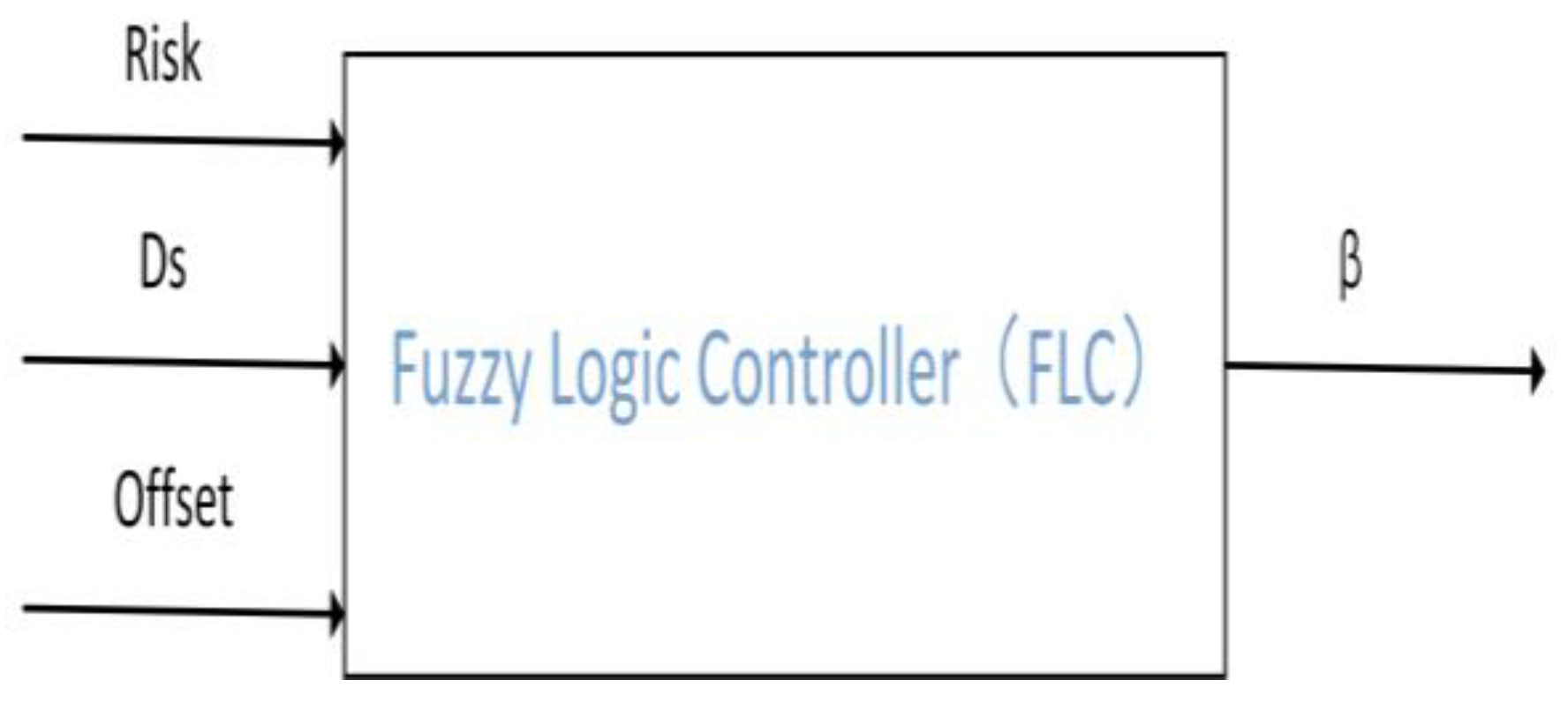
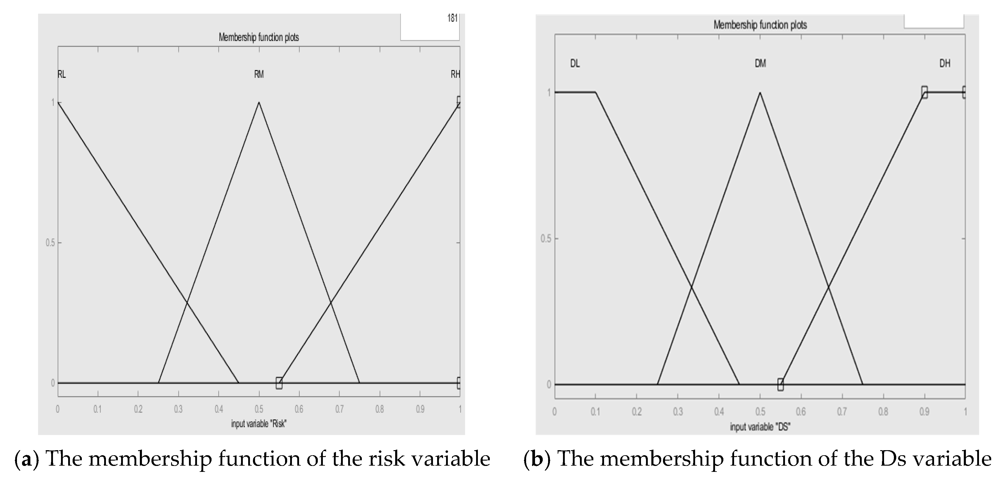
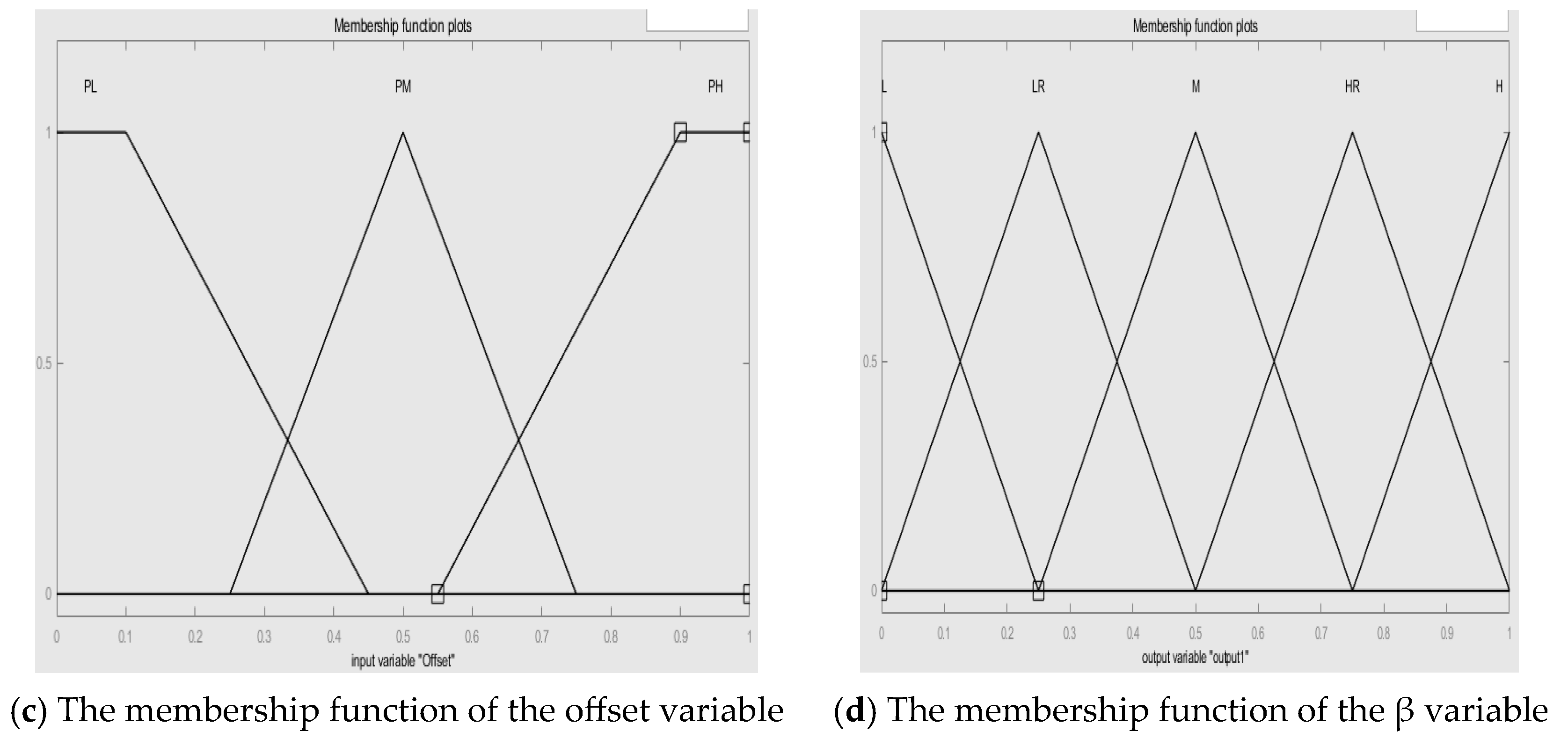
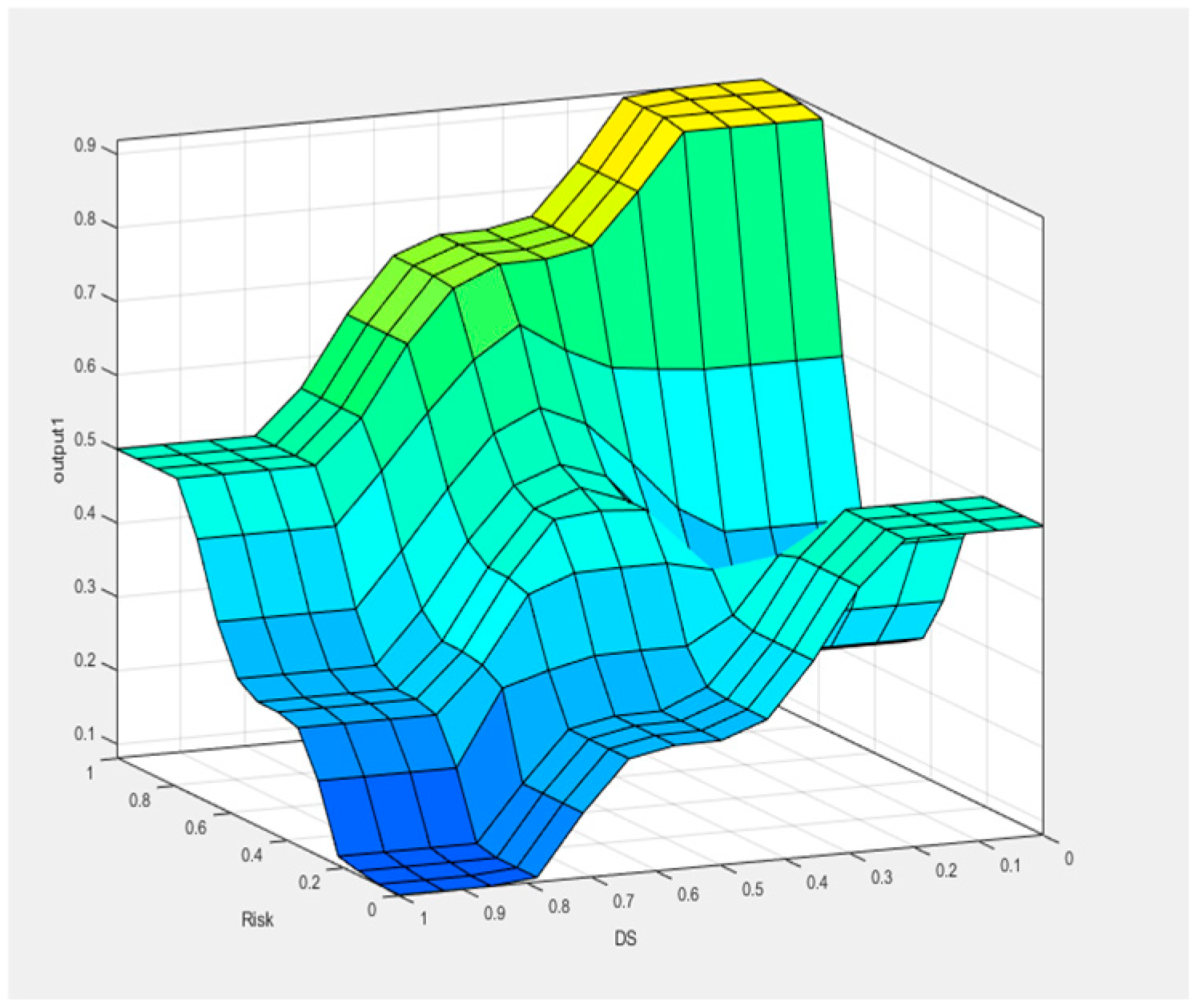
3.2.3. Dynamic Weight Adjustment of Driving Authority Based on Fuzzy Rules

The deviation between the driving risk and the global controller directly impacts the driving weight distribution between the human driver and the automated system. Nevertheless, it remains challenging to formulate an analytical mathematical relationship between this deviation and the variation in driving weight. Specifically, when the driving risk is elevated and the driver’s state is suboptimal, it is desirable to increase the driving weight of the co-driving controller. This augmentation of its intervention level serves to safeguard driving safety. Conversely, when the driving risk is relatively low, the driving weight of the vehicle should be transferred to the driver, ensuring that the vehicle adheres to the driver’s control commands. Therefore, on the premise of ensuring safe driving operations, it is essential to offer more assistance to drivers in a poor state and minimize intervention for those in a good state. This approach aims to alleviate the driver’s workload and enhance overall driving performance and safety.

A fuzzy logic controller is employed to design the weights. The structure of the fuzzy logic controller is depicted in Figure 5. Herein, the driving environment risk $Risk$, the global control deviation $Offset$, and the driver’s state $Ds$ serve as the inputs, while the weight $\beta$ of the autonomous driving system acts as the output.

The driving environment risks and deviations in global control can be obtained via the methods described above. The state of the human driver can be obtained by monitoring the driver’s physiological signals or operational behaviors related to the vehicle. Moreover, the driver model can be simulated using state parameters.

The triangular membership function features a simple structure, low computational complexity, and high sensitivity. Its vertices correspond to typical values, facilitating adjustment. In this study, the triangular membership function is employed to characterize the fuzzy set. Regarding situations where the values of $Ds$ and $Offset$ are either relatively large or relatively small, a semi-trapezoidal membership function is utilized for the description. The semi-trapezoidal function is capable of effectively dealing with boundary conditions. It helps to circumvent blind spots in the rules, thereby ensuring that even the maximum value of $D_s$ or the minimum value of $Offset$ can still activate the corresponding rules. Finally, the membership functions for each input and output variable are presented in Figure 6.

Each fuzzy rule is associated with a fuzzy relation. The fuzzy relation $Ri$ corresponding to the $i$-th rule is expressed as

$$R_i={(Ris{k}_l\times D{s}_m\times Offse{t}_n)}^{T_1}\times {\beta }_k$$

(50)

Among them, $i\in \{1,2,3,\dots ,7\},l,m,n\in \{1,2,3\},k\in \{1,2,3,4,5\},T_l$ is the transfer matrix of column vectors.

The synthetic inference rule is adopted to calculate the fuzzy output. Then, the defuzzification of the output fuzzy quantity is carried out using the centroid method, from which a corresponding crisp output value can be obtained. As depicted in Figure 7.

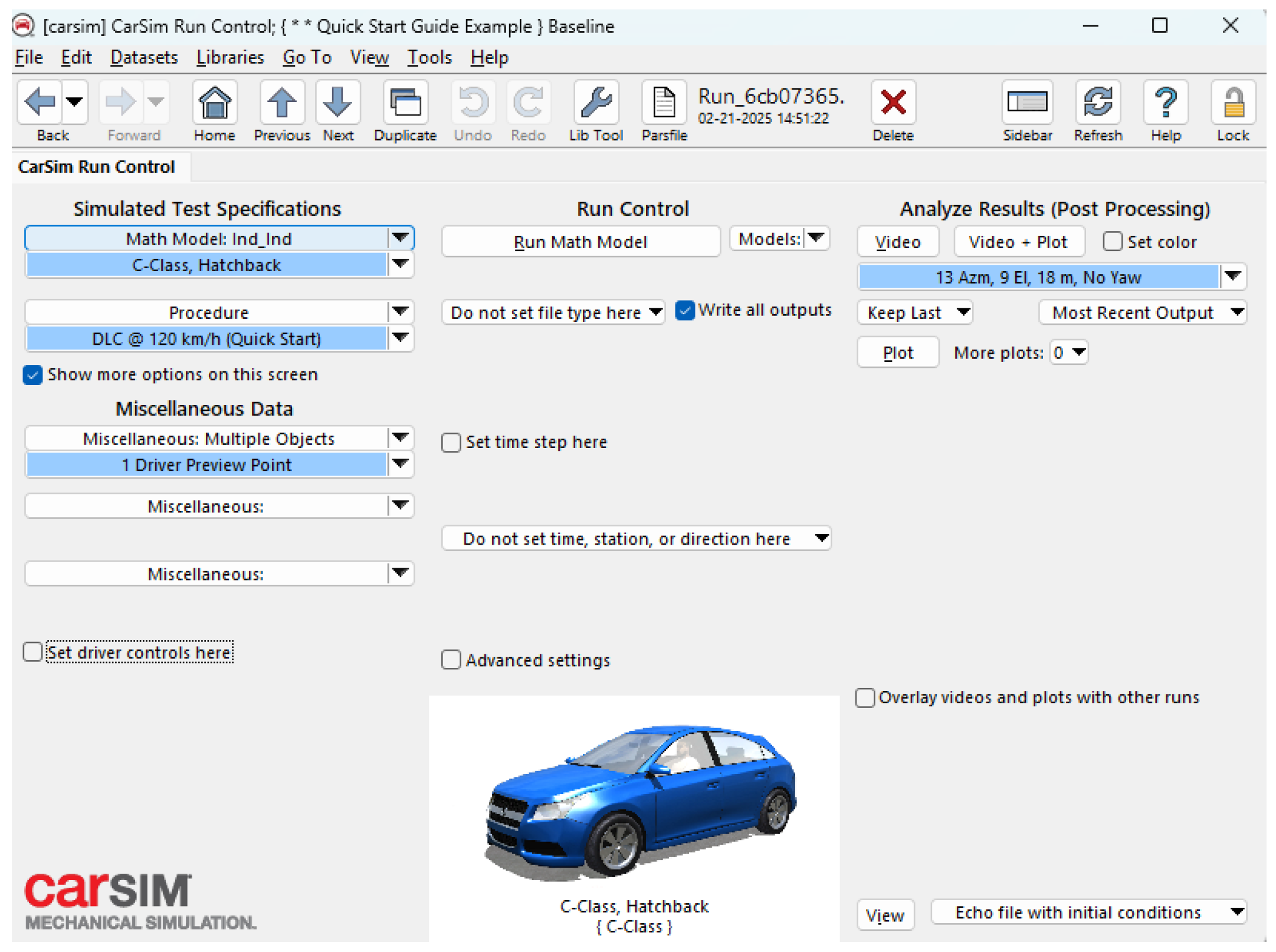
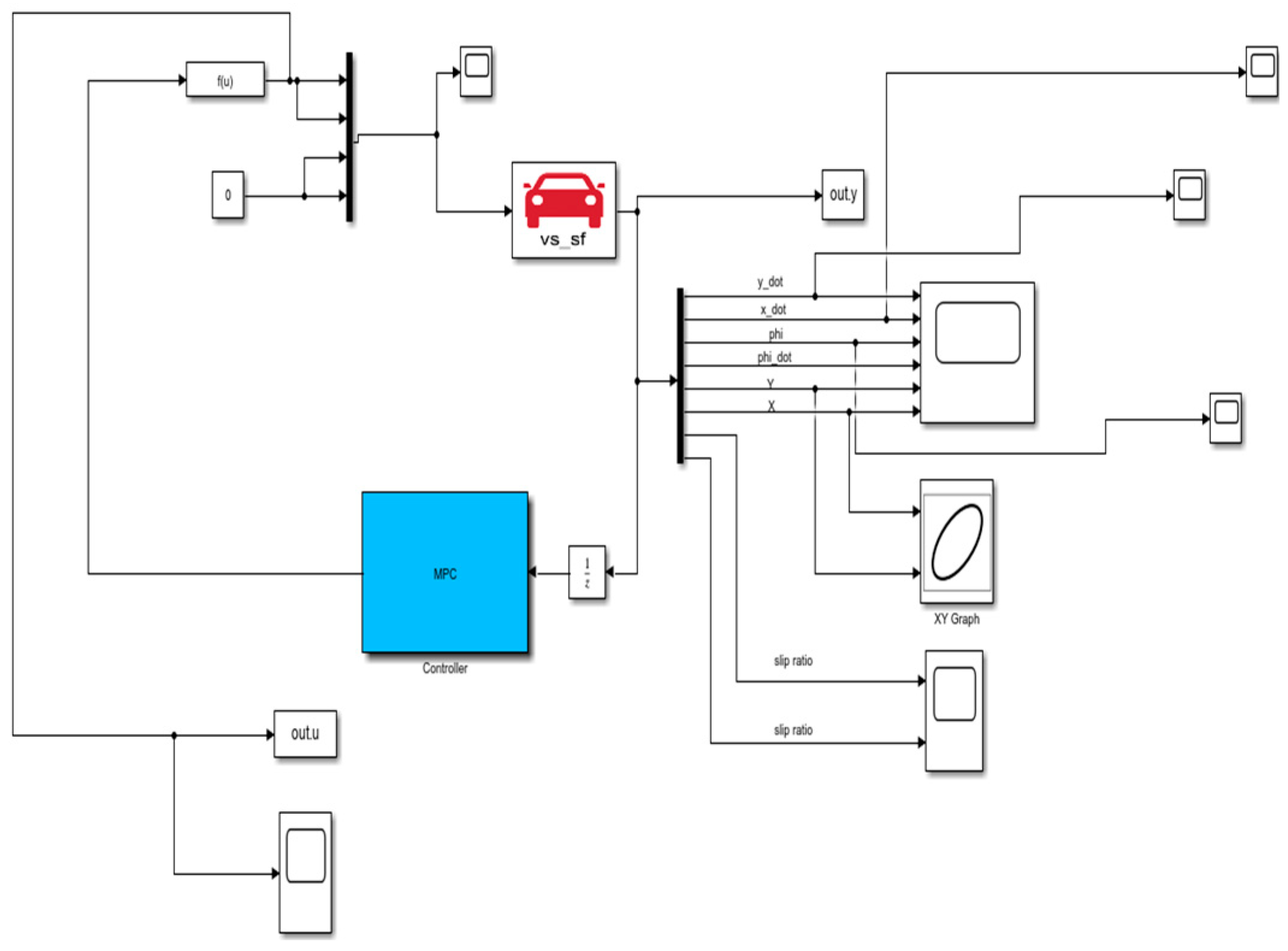
4. Simulation Results and Their Analysis

As depicted in Figure 8, the scenario under consideration is a stretch of a two-lane highway, where each lane has a width of 3.5 m, and the speed of the vehicle $V_s$ is 60 km/s, while that of the vehicle $V_f$ is 70 km/s. All vehicles are located on the centerline of the lane. To assess the effectiveness of dynamic weight allocation within risk scenarios, two obstacle vehicles are introduced into the experimental scenario. The ego vehicle $V_s$ is traveling at a constant speed while following the leading vehicle $V_f$ in the right-hand lane. There is a stationary obstacle (accident vehicle $V_{o1}$) 100 m ahead in the ego vehicle’s lane and another stationary obstacle (accident vehicle $V_{o2}$) 150 m ahead in the left-hand lane. Nevertheless, owing to occlusion by the leading vehicle, the driver of the ego vehicle fails to recognize the danger. At a particular instant, the leading vehicle abruptly changes lanes. Subsequently, the driver of the ego vehicle spots the obstacles on the lanes and initiates an emergency obstacle avoidance operation. To validate the steering interaction, it is specified that all drivers uniformly implement the lane-changing obstacle avoidance strategy. During the co-simulation of CarSim and Simulink in the context of human–machine collaborative driving, two operating conditions are applied separately: solely the driver driving and human–machine collaborative driving.

The results of the experimental simulation are presented in Figure 9 and Figure 10. Specifically, Figure 9 depicts the outcomes of driver A’s participation in driving, and Figure 10 shows those of driver B’s involvement. Here, $D{A}_a$ and $D{A}_b$ denote the driving conditions of driver A and driver B operating independently, respectively. Meanwhile, $S{C}_a$ and $S{C}_b$ represent collaborative driving conditions where driver A and driver B cooperate with the autonomous driving system, respectively.

By contrasting the curves for various indicators when the drivers are driving solo in Figure 9 and Figure 10, it can be observed that driver A demonstrates a superior driving state to that of driver B. For driver A, the driving trajectory and the control input variables exhibit smooth variations. Specifically, the peak value of the yaw rate is maintained below 0.25 rad·s⁻¹, which indicates that driver A is capable of accurately fulfilling the driving task. In contrast, driver B fails to successfully execute the steering and obstacle avoidance tasks. Notably, at the longitudinal position of X = 100 m, driver B comes perilously close to colliding with the road boundary.

Regarding driver A, the trajectory during collaborative driving with the autonomous driving system approximately coincides with that during solo driving. As can be observed from Figure 9b, the weight of the autonomous driving system generally remains at around 0.1. Only when entering high-risk areas does the weight increase slightly, yet it still remains below 0.2. This suggests that driver A maintains a relatively high driving weight and a high level of driving freedom throughout the collaborative process.

Concerning driver B, owing to the suboptimal driving state, the initial driving weight assigned to the autonomous driving system is relatively higher. Consequently, when solving the non-cooperative interaction model, a greater advantage can be achieved. This enables more substantial intervention in the vehicle’s operation to help the driver complete their steering maneuvers.

As depicted in Figure 10b, the weight adjustment strategy proposed in this section effectively mitigates drastic fluctuations in the driving weights between the human driver and the autonomous driving system. During the first lane-changing process, taking into account the driver’s state, the driving weight of the autonomous driving system only experiences a minor increase when the vehicle reaches the longitudinal position of X = 50 m, which is attributed to the relatively high environmental risk at that moment. During the second lane-changing process, when the vehicle reaches the longitudinal position of X = 96 m, despite a rapid surge in risk, the weight of the autonomous driving system only shows a marginal change. This is because the global control deviation remains within a narrow range. When the driver is in a less-than-ideal state, minimizing significant weight variations can effectively alleviate the driver’s psychological stress and operational burden. As is evident from Figure 10a, the vehicle’s driving path during collaborative driving is smoother. Additionally, as shown in Figure 10c, the collaborative driving mode significantly reduces the driver’s large-scale control inputs, thereby decreasing the driver’s level of exertion.

In view of the overall outcomes of the aforementioned simulation experiments, during the collaborative driving process, the degree of driver effort is lower, and the vehicle exhibits a lower yaw angular velocity. This indicates that the collaborative driving strategy can assist drivers in alleviating their driving burden and enhancing driving safety. When comparing the results of collaborative driving among different drivers, the proposed strategy can provide varying degrees of assistance to drivers in different states, thereby ensuring driving freedom. In contrast to a strategy that solely relies on environmental risks to adjust the driving weights, the proposed adaptive weight decision-making model can yield weights with a smaller range of variation. This is more conducive to enabling drivers to understand their driving characteristics and promoting the achievement of equilibrium in the human–machine interaction, thus reducing driver discomfort.

5. General Conclusions

This paper presents a human–machine collaborative steering control method grounded in the leader–follower game theory. Taking into account the characteristics of unconscious human–machine competition, the human–machine interaction is characterized as a leader–follower game relationship. Through the application of backward induction, the optimal control strategy under equilibrium conditions is theoretically derived. This enables the conditions for achieving game equilibrium to be determined and the optimal human–machine control strategy that incorporates the ability for dynamic adjustment to the driving authority under such equilibrium to be formulated. Subsequently, an adaptive weight decision-making model based on fuzzy control rules is designed. This model modifies the conditions for human–machine game equilibrium to fulfill the path-tracking task. In this adaptive weight decision-making model, a globally optimal steering controller is innovatively introduced. This controller serves to monitor the stability of human–machine control. Additionally, a fuzzy controller is constructed by integrating the traffic environment risks and the driver’s state, thereby realizing dynamic adjustments of human–machine driving authority.

The experimental results demonstrate that the proposed method can effectively alleviate the driver’s workload, enhance the stability of vehicle motion, and assist drivers in diverse states to accomplish driving tasks. In comparison with strategies that merely adjust the driving weights according to risk factors, the adaptive weight decision-making model proposed in this study exhibits smaller fluctuations in the weight values. When applying game theory to addressing conflict issues, smaller weight variations are more conducive to reaching equilibrium, causing less disruption to the human–machine balance and reducing driver discomfort. Existing studies have primarily focused on collaborative steering control of drivers and controllers, yet they have overlooked the latent cooperative potential in longitudinal control. In future research, intelligent driving vehicles will generally need to execute both lateral and longitudinal control simultaneously to cope with more complex traffic scenarios.

From the analytical expression of the leader–follower game equilibrium control strategy derived, it can be seen that the optimal human–machine steering control strategy within the leader–follower collaborative framework is directly associated with the driving intentions of both the human and the machine; the vehicle’s state; and the driving weights. Accurate extraction of the driver’s driving intentions and the rational selection of the driving weights have a direct bearing on the performance of the human–machine hybrid system. Therefore, future research should be centered on improving the ability to predict driver intentions, along with the application of reinforcement learning to the field of intelligent driving [22,23,24]. For instance, reinforcement learning can be employed as the driving system for intelligent vehicles in specific scenarios. This approach aims to enhance the overall performance of the human–machine co-driving system further. The development of high-fidelity traffic models for simulating the social behavior of vehicles in traffic scenarios is conducive to the preliminary calibration of the parameters of the control algorithms for intelligent driving vehicles. This approach can effectively save development time and effort. In this study, only joint simulation verification was conducted, which has certain deficiencies in practical engineering applications. Specifically, the control performance of the designed control strategy has not been verified through hardware-in-the-loop bench tests with drivers or in real vehicles. In future hardware-in-the-loop tests, the following aspects need to be addressed: first, the encapsulation of the controller model and code generation; second, the deployment on real-time platforms to achieve real-time operation of the controller on physical hardware; third, the establishment of software and hardware interfaces for signal interaction with the virtual vehicle dynamics model to form a closed-loop operation; and fourth, data collection and performance evaluation to ensure that the system meets the requirements of embedded deployment and real-time performance. This will promote its application in actual intelligent driving systems.

References

1. Tang, F.; Gao, F.; Wang, Z. Driving Capability-Based Transition Strategy for Cooperative Driving: From Manual to Automatic. IEEE Access 2020, 8, 139013–139022. [Google Scholar] [CrossRef]
2. Gao, F.; He, B.; He, Y. Detection of Driving Capability Degradation for Human-Machine Cooperative Driving. Sensors 2020, 20, 1968. [Google Scholar] [CrossRef]
3. Wu, J.; Kong, Q.; Yang, K.; Liu, Y.; Cao, D.; Li, Z. Research on the Steering Torque Control for Intelligent Vehicles Co-Driving With the Penalty Factor of Human–Machine Intervention. IEEE Trans. Syst. Man Cybern. Syst. 2023, 53, 59–70. [Google Scholar] [CrossRef]
4. Xing, Y.; Lv, C.; Cao, D.; Hang, P. Toward human-vehicle collaboration: Review and perspectives on human-centered collaborative automated driving. Transp. Res. Part C Emerg. Technol. 2021, 128, 103199. [Google Scholar] [CrossRef]
5. Fang, Z.; Wang, J.; Wang, Z.; Liang, J.; Liu, Y.; Yin, G. A Human-Machine Shared Control Framework Considering Time-Varying Driver Characteristics. IEEE Trans. Intell. Veh. 2023, 8, 3826–3838. [Google Scholar] [CrossRef]
6. Xu, Q.; Zhang, X.; Lei, Z.; Wen, G.; Li, X.; Su, Y.; Gu, S. Robust path-tracking control for intelligent vehicles considering human–vehicle multi-factors. J. Vib. Control. 2025. [Google Scholar] [CrossRef]
7. Xie, W.; Lu, S.; Dai, L.; Jia, R. Interactive strategy of shared control vehicle and automated vehicles based on adaptive non-cooperative game. Proc. Inst. Mech. Eng. Part D J. Automob. Eng. 2024. [Google Scholar] [CrossRef]
8. Zhao, X.; Yin, Z.; He, Z.; Nie, L.; Li, K.; Kuang, Y.; Lei, C. Indirect Shared Control Strategy for Human-Machine Cooperative Driving on Hazardous Curvy Roads. IEEE Trans. Intell. Veh. 2023, 8, 2257–2270. [Google Scholar] [CrossRef]
9. Liu, J.; Guo, H.; Meng, Q.; Shi, W.; Gao, Z.; Chen, H. Game-Theoretic Driver-Automation Cooperative Steering Control on Low-Adhesion Roads With Driver Neuromuscular Delay. IEEE Trans. Intell. Transp. Syst. 2024, 25, 10115–10130. [Google Scholar] [CrossRef]
10. Dai, C.; Zong, C.; Zhang, D.; Hua, M.; Zheng, H.; Chuyo, K. A Bargaining Game-Based Human–Machine Shared Driving Control Authority Allocation Strategy. IEEE Trans. Intell. Transp. Syst. 2023, 24, 10572–10586. [Google Scholar] [CrossRef]
11. Zhou, Y.; Huang, C.; Hang, P. Game Theory-Based Interactive Control for Human–Machine Cooperative Driving. Appl. Sci. 2024, 14, 2441. [Google Scholar] [CrossRef]
12. Feng, J.; Yin, G.; Liang, J.; Lu, Y.; Xu, L.; Zhou, C.; Peng, P.; Cai, G. A Robust Cooperative Game Theory-Based Human–Machine Shared Steering Control Framework. IEEE Trans. Transp. Electrif. 2024, 10, 6825–6840. [Google Scholar] [CrossRef]
13. Lu, X.; Zhao, H.; Li, C.; Gao, B.; Chen, H. A Game-Theoretic Approach on Conflict Resolution of Autonomous Vehicles at Unsignalized Intersections. IEEE Trans. Intell. Transp. Syst. 2023, 24, 12535–12548. [Google Scholar] [CrossRef]
14. Liu, M.; Wan, Y.; Lewis, F.L.; Nageshrao, S.; Filev, D. A Three-Level Game-Theoretic Decision-Making Framework for Autonomous Vehicles. IEEE Trans. Intell. Transp. Syst. 2022, 23, 20298–20308. [Google Scholar] [CrossRef]
15. Liu, M.; Kolmanovsky, I.; Tseng, H.E.; Huang, S.; Filev, D.; Girard, A. Potential Game-Based Decision-Making for Autonomous Driving. IEEE Trans. Intell. Transp. Syst. 2023, 24, 8014–8027. [Google Scholar] [CrossRef]
16. Li, G.; Tian, T.; Song, J.; Li, N.; Bai, H. Research on trajectory tracking control of driverless cars based on game theory. Proc. Inst. Mech. Eng. Part D J. Automob. Eng. 2024, 239, 1536–1553. [Google Scholar] [CrossRef]
17. Wang, H.; Zheng, W.; Zhou, J.; Feng, L.; Du, H. Intelligent vehicle path tracking coordinated optimization based on dual-steering cooperative game with fault-tolerant function. Appl. Math. Model. 2024, 139, 115808. [Google Scholar] [CrossRef]
18. Gong, J. Model Predictive Control of Unmanned Vehicles; Beijing Institute of Technology Press Co., Ltd.: Beijing, China, 2020. [Google Scholar]
19. Guo, K.; Guan, H. Modelling of driver/vehicle directional control system. Veh. Syst. Dyn. 1993, 22, 141–184. [Google Scholar] [CrossRef]
20. Rasekhipour, Y.; Khajepour, A.; Chen, S.K.; Litkouhi, B. A potential field-based model predictive path-planning controller for autonomous road vehicles. IEEE Trans. Intell. Transp. Syst. 2016, 18, 1255–1267. [Google Scholar] [CrossRef]
21. Wakasugi, T. A study on warning timing for lane change decision aid systems based on driver’s lane change maneuver. In Proceedings of the 19th International Technical Conference on the Enhanced Safety of Vehicles, Washington, DC, USA, 6–9 June 2005. Paper No. 05-0290. [Google Scholar]
22. Wang, S.; Jia, D.; Weng, X. Deep reinforcement learning for autonomous driving. arXiv 2018, arXiv:1811.11329. [Google Scholar]
23. Tseng, K.-K.; Yang, H.; Wang, H.; Yung, K.L.; Lin, R.F.Y. Autonomous driving for natural paths using an improved deep reinforcement learning algorithm. IEEE Trans. Aerosp. Electron. Syst. 2022, 58, 5118–5128. [Google Scholar] [CrossRef]
24. Islam, F.; Ball, J.E.; Goodin, C.T. Enhancing longitudinal velocity control with attention mechanism-based deep deterministic policy gradient (DDPG) for safety and comfort. IEEE Access 2024, 12, 30765–30780. [Google Scholar] [CrossRef]
Figure 1. The human–machine master–slave Game-Based cooperative control structure with adaptive weights.
Wevj 16 00386 g001
Figure 2. Three-degree-of-freedom vehicle model.
Wevj 16 00386 g002
Figure 3. An image of the CarSim interface.
Wevj 16 00386 g003
Figure 4. A control diagram of MPC.
Wevj 16 00386 g004
Figure 5. The structure of the fuzzy logic controller.
Wevj 16 00386 g005
Figure 6. The membership functions of the variables in the fuzzy logic controller.
Wevj 16 00386 g006aWevj 16 00386 g006b
Figure 7. Driving weight surface.
Wevj 16 00386 g007
Figure 8. A schematic illustration of the experimental scenario.
Wevj 16 00386 g008
Figure 9. The simulation results of the model for driver A. (a) Travel trajectory, (b) the curve of the variation in the FLC variable, (c) the degree of the driver’s effort, and (d) yaw rate.
Wevj 16 00386 g009
Figure 10. The simulation results of the model for driver B. (a) Travel trajectory, (b) the curve of the variation in the FLC variable, (c) the degree of the driver’s effort, and (d) yaw rate.
Wevj 16 00386 g010