Dynamic Simulation of Ground Braking Force Control Based on Fuzzy Adaptive PID for Integrated ABS-RBS System with Slip Ratio Consideration

Abstract

This study resolves a critical challenge in electromechanical brake system validation: conventional ABS/RBS integrated platforms’ inability to dynamically simulate tire-road adhesion characteristics during braking. We propose a fuzzy adaptive PID-controlled magnetic powder clutch (MPC) system that achieves ground braking force simulation synchronized with slip ratio variations. The innovation encompasses: (1) Dynamic torque calculation model incorporating the curve characteristics of longitudinal friction coefficient ($\phi$) versus slip ratio ($s$), (2) Nonlinear compensation through fuzzy self-tuning PID control, and (3) Multi-scenario validation platform. Experimental validation confirms superior tracking performance across multiple scenarios: (1) Determination coefficients R² of 0.942 (asphalt), 0.926 (sand), and 0.918 (snow) for uniform surfaces, (2) R² = 0.912/0.908 for asphalt-snow/snow-asphalt transitions, demonstrating effective adhesion characteristic simulation. The proposed control strategy achieves remarkable precision improvements, reducing integral time absolute error (ITAE) by 8.3–52.8% compared to conventional methods. Particularly noteworthy is the substantial ITAE reduction in snow conditions (236.47 vs. 500.969), validating enhanced simulation fidelity under extreme road surfaces. The system demonstrates consistently rapid response times. These improvements allow for highly accurate replication of dynamic slip ratio variations, establishing a refined laboratory-grade solution for EV regenerative braking coordination validation that greatly enhances strategy optimization efficiency.

1. Introduction

The co-existence of regenerative braking systems (RBS) and anti-lock braking systems (ABS) in electric vehicles (EVs) creates a critical control paradox: maximizing energy recovery while ensuring wheel stability during emergency braking. Industry reports indicate predominant energy losses during ABS-RBS interaction phases [1], primarily due to transient torque conflicts between electrical and hydraulic braking subsystems. This challenge is exacerbated by the lack of test platforms capable of simulating dynamic tire-road adhesion characteristics, a prerequisite for validating next-generation coordinated control strategies.

Traditional bench testing systems face two fundamental limitations:

(1)

Static adhesion modeling using fixed $\phi -s$ curves [2,3,4,5], incapable of replicating real-time slip dynamics;

(2)

The open-loop control of a magnetic powder clutch (MPC) can’t meet the needs of the dynamic torque changes of an MPC in a test bench [6,7,8,9];

(3)

Lack of integrated platforms for synchronous ABS/RBS performance evaluation.

Our work addresses these gaps through three innovations:

(1)

$\phi -s$ Adaptive Control: Dynamic torque regulation based on real-time slip ratio with threshold switching between $T_p$ and $T\left(s\right)$.

(2)

Self-Tuning Fuzzy PID Control: Two-dimensional rule-based adaptation with 49-rule Mamdani inference for hysteresis compensation.

(3)

Cross-Surface Validation: Integrated testing of uniform and $\phi$-jump conditions with adaptive $T_p/T\left(s\right)$ switching.

Experimental validation demonstrates 91–94% fidelity in reproducing asphalt-to-snow adhesion transitions, establishing a new benchmark for braking strategy development. The subsequent literature review systematically analyzes technological barriers across control strategies, validation methods, and actuator dynamics.

2. Literature Review

The synergistic integration of regenerative and anti-lock braking systems remains pivotal for advancing electric vehicle safety and energy efficiency. While substantial progress has been made in coordinated control strategies, three critical knowledge gaps persist: (1) limited experimental validation of multi-$\phi$ condition adaptability, (2) oversimplified tire-road interaction modeling in bench testing, and (3) inadequate dynamic response in conventional clutch control systems. This review systematically traces the progression from theoretical simulations to hardware-in-the-loop validation, ultimately exposing the fundamental disconnect between static bench configurations and real-world $\phi -s$ dynamics—a deficiency directly addressed through our adaptive magnetic clutch control framework.

2.1. Theoretical Validation and Simulation Studies

Early studies primarily validated control strategies through simulation. H.J. et al. [10] proposed a fuzzy logic-based coordination method for RBS and ABS, achieving system coordination through dual independent fuzzy controllers. Y.Y. et al. [11] developed a closed-loop integrated wheel slip control system that maintained traditional ABS braking distances while enabling energy recovery. Q.X. et al. [12] innovatively introduced EMCB/DMB dual-mode braking strategies, achieving target slip ratio tracking (RMSE < 0.02) via predictive algorithms. J.B. et al. [13] designed a braking force distribution algorithm considering motor and battery characteristics to optimize front/rear axle force ratios. S. H. et al. [14] proposed a braking strategy for a dual-motor all-wheel-drive (AWD) electric vehicle (EV) that utilizes real-time sensing of DC bus current in each motor controller to achieve optimal braking distribution between friction braking and regenerative braking. C. L. et al. [15] introduced a coordinated braking algorithm based on nonlinear model predictive control (NMPC), with optimization objectives including energy recovery rate, tire slip ratio, and motor torque variation. Under the WLTC (Worldwide Harmonized Light Vehicles Test Cycle) conditions, this approach achieved a 30.4% energy recovery rate while ensuring braking safety through slip ratio control. However, these studies did not account for the influence of diverse road conditions.

To address road adaptability, H.L. et al. [16] proposed a Regenerative and Hydraulic Braking Coordination Strategy (RRBCS) based on optimal slip ratio (OSR), achieving I-curve tracking through front/rear wheel slip ratio adjustments. Y.Y. et al. [17] integrated logic threshold and phase plane theory to ensure motor torque remains within the ABS steady-state range during activation. Y.Y. et al. [18] validated the MPC strategy’s stability improvements in Carsim through high/low adhesion rear-end collision scenarios. K.V. et al. [19] proposed series and parallel cooperative braking strategies to investigate the impact of regenerative braking torque blend-out on the braking performance of electrified heavy vehicles, while C.X. et al. [20] completed HIL platform tests covering five road types, including split-μ and turning surfaces. K.V.S. et al. [21] developed a cooperative braking strategy with optimal braking force distribution between regenerative braking and friction braking to enhance cornering stability and handling performance of electric heavy-duty commercial vehicles during combined braking and steering maneuvers. The strategy was validated under various road conditions, including dry pavement and snow-covered surfaces. To address the tire slip control problem, M. Melendez-Useros et al. [22] developed an H∞ controller. This controller sets target slip ratios based on road friction coefficients for different road adhesion conditions. Its effectiveness was validated in CarSim vehicle dynamics simulations. The tests demonstrated that the controller can accurately track the target slip ratios, exhibiting small tracking errors and good transient responses across the tested road conditions. Peter Girovsky et al. [23] proposed a fuzzy logic-based optimization method for Anti-lock Braking Systems (ABS) to address precise slip ratio control under diverse road conditions. By establishing a vehicle-wheel speed dynamic coupling model, they designed a dual-input (normalized vehicle speed, wheel-to-vehicle speed ratio) fuzzy controller centered on real-time slip ratio λ. This controller enforced slip ratio stabilization at a fixed threshold of 20% on both dry roads and asymmetric split-μ roads (left/right wheel adhesion coefficients μ = 0.2/0.5). Simulation results demonstrated a 76% reduction in slip ratio fluctuation amplitude compared to conventional ABS during braking at 140 km/h on split-μ surfaces—indicating enhanced directional stability—thereby validating the fixed-threshold strategy’s effectiveness under extreme asymmetric conditions. However, the absence of a road parameter adaptation mechanism in the fuzzy rules prevents dynamic adjustment of the optimal slip ratio according to μ variations (e.g., typically <10% on icy surfaces), limiting its applicability across diverse road surfaces. Additionally, M. Vignati et al. [24] presented a Force-based Braking Control Algorithm (FBA) for vehicles with electric motors. By adjusting the output torque of the electric motor, the FBA regulates the braking force applied to the wheel. Simulations on surfaces with high and low adhesion coefficients, as well as sudden changes in adhesion (e.g., puddles), have verified that the FBA significantly enhances braking performance and vehicle safety. M.S. et al. [25] propose a coordinated control strategy for a blended regenerative anti-lock braking system (RABS) and electronic wedge brake (EWB) in all-wheel-motor-drive electric vehicles. By employing accurate vehicle dynamics and tire models, along with a dynamic braking force distribution strategy, the proposed method achieves precise simulation and optimization of the ground braking force.

2.2. Evolution of Experimental Validation Methods

2.2.1. Road Test Validation

Real-world testing became critical for strategy verification. Y.S. et al. [26] proposed an ABS road-condition identification algorithm, which was validated through track tests demonstrating its high efficiency and accuracy in detecting significant changes in tire-road friction conditions. J.S. et al. [27] designed an ABS for distributed-drive EVs based on regenerative braking. Through road tests, its braking performance and energy recovery efficiency on different road conditions were verified. MPC was used to allocate torque between hydraulic and electric braking, with the optimal slip ratio as the control target. However, the study mainly focused on low-intensity braking conditions. Q.Z. et al. [28] enhanced inter-axle force distribution accuracy through fuzzy-sliding mode hybrid control verified by simulations and experiments. F.J. et al. [29] achieved dynamic balance between braking stability and energy recovery on ice/cement surfaces. C.S. Nanda Kumar et al. [30] proposed a novel coordinated control strategy called ‘combined braking’ for regenerative braking and friction braking. Real-vehicle tests on dry asphalt roads demonstrated that the energy recovery of combined braking approaches is nearly twice that of parallel braking. L.Z. et al. [31] introduced a cooperative control strategy for regenerative braking and friction braking during ABS activation transients, based on a probability index (f) for ABS triggering. Simulation and real-vehicle road tests showed that regenerative braking decreases as the index increases, thereby improving braking safety and driving comfort during ABS activation transients.

2.2.2. Bench Testing Advancements

Bench testing demonstrated higher repeatability than road tests [32]. A.A et al. [2] developed a hardware-in-the-loop (HIL) test platform and employed the Ostermeyer model to evaluate the performance of an anti-lock braking system (ABS). The Ostermeyer model dynamically simulates the friction coefficient of brake linings, taking into account the effects of velocity, pressure, and temperature. Although the model can adjust the friction coefficient in real-time to accommodate varying driving conditions, it does not explicitly simulate the impact of slip ratio variations on the friction coefficient. D. Tavernini et al. [3] designed an eNMPC ABS controller for an EHB system, utilizing the Pacejka Magic Formula tire model to determine the optimal reference slip ratios. For high friction conditions (µ = 0.9), a fixed maximum reference slip ratio of 0.07 was adopted, while for low friction conditions (µ = 0.45), a fixed maximum reference slip ratio of 0.04 was used. In the study by Heydari et al. [33], a hardware-in-the-loop (HIL) experimental test bench was employed to simulate the ground braking forces for evaluating an electric vehicle’s (EV) regenerative braking strategy. The setup featured two high-performance permanent magnet synchronous motors (PMSMs) connected to a common shaft, with one motor emulating the EV’s traction motor and the other acting as a dynamometer (DYNO) to impose braking forces. However, the research did not specifically address the simulation of ground braking forces varying with slip ratio during braking.

Existing test benches are predominantly limited to simulating only single operating conditions, as they typically preset a fixed braking torque value in magnetic powder clutches based on maximum adhesion force [8]. This approach fundamentally restricts their capability to simulate variable road conditions. Moreover, even for single-condition simulations, the ground braking force is represented as a constant value. While magnetic powder clutches exhibit a linear current-torque relationship in static characteristics, their open-loop control cannot compensate for hysteresis effects, resulting in deviations in braking force-slip ratio dynamics [9]. K.V.S. et al. [34] established optimal slip ratio ranges (0.15–0.2/0.1–0.15/0.06–0.1/0.04–0.06) corresponding to different road friction coefficients (μ = 0.8/0.5/0.35/0.2). By treating regenerative braking as a discontinuous control variable to dynamically adjust driven wheel braking force while maintaining a linear braking force distribution (BFD) ratio, this approach overcomes the slip control limitations inherent in conventional fixed regenerative braking strategies. X.X. et al. [35] designed a single-wheel all-electric ABS test bench. It adjusts wheel braking force by controlling the electromagnetic mechanical brake’s (EMB) output torque, simulating wheel dynamics under varying initial speeds and road adhesion coefficients.

2.3. Technical Challenges in Bench Testing

The first-order inertial characteristics of magnetic powder clutches (transfer functions with time-delay terms) induce steady-state errors in traditional open-loop control. Most studies applied constant currents based on preset maximum adhesion, resulting in slip-independent braking forces that misrepresent tire-road adhesion. Although intelligent control algorithms improved tracking performance compared to open-loop methods, dynamic multi-condition simulation capabilities remain insufficient.

The remainder of this paper is organized as follows: Section 3 presents the architecture of the integrated ABS and RBS control test platform for electric vehicles. Section 4 details the simulation design for ground braking force estimation. Experimental results are provided in Section 5, followed by a discussion of the findings in Section 6. Finally, Section 7 concludes the paper.

3. Structure of the Integrated Control Test Platform for Electric Vehicle ABS and RBS

The structure of the integrated control test platform for electric vehicle ABS and RBS is illustrated in Figure 1 below.

3.1. Drive Motor and Its Control System

The drive motor is one of the core components of the integrated control test platform for ABS and RBS of electric vehicles. It is used to simulate the power output during vehicle operation and energy recovery during regenerative braking. A permanent magnet synchronous motor (PMSM) is effective in electric driving mobility. The test platform employs a PMSM model Z4-112/4-2 (Xi’an Hongtai Motor Co., Ltd., Xi’an, China), equipped with a cooling device.

3.2. Inertial Mass Simulation System

The test platform uses a flywheel assembly to simulate the inertial mass of the vehicle. The rotational kinetic energy of the flywheel assembly simulates the translational kinetic energy of a vehicle in motion. The flywheel assembly consists of six flywheel units with different masses, capable of simulating vehicle masses of 1000 kg, 500 kg, 250 kg, 125 kg, 62.5 kg, and 31.25 kg, respectively. By combining different flywheel units, the platform can simulate vehicles with masses ranging from a minimum of 93.75 kg to a maximum of 1968.75 kg, with a step size of 31.25 kg.

3.3. Braking System

The integrated control platform allocates regenerative braking force and mechanical braking force based on braking intensity requirements and the braking torque distribution strategy. In the integrated control of ABS and RBS, ABS and RBS need to work in coordination. To precisely control the brake pedal travel and mechanical braking force, the test platform is equipped with a brake-by-wire system. This system includes a brake travel simulator, a brake travel sensor measurement system, and a mechanical hydraulic brake. The brake travel simulator, as shown in Figure 2, consists of an electric pushrod device and its drive controller. The electric pushrod contains a stepper motor, and the drive controller controls the motor to achieve the motion of the pushrod. The pushrod is connected to a vacuum booster. During operation, the drive controller receives commands via the CAN bus, controls the motor to drive the pushrod, and moves the piston in the master cylinder. The vacuum booster amplifies the pushrod’s thrust using vacuum pressure, causing the friction elements in the disc brake to clamp the brake disc under hydraulic pressure, thereby generating braking force and decelerating the flywheel on the test platform. The working parameters of the pushrod are listed in

Table 1. Working parameters of the electric push rod.

Electric Cylinder Model	Effective Stroke	Maximum Speed	Maximum Thrust
RCP2-RA4C-I-42P-10-300-P1-R04-B	350 mm	350 mm/s	250 N

. The Electric Cylinder was provided by Dongguan Suli Automation Technology Co., Ltd. (Dongguan, China).

3.4. Hybrid Energy Storage System

The test platform employs a dual-energy storage system consisting of a power battery pack and a supercapacitor, as illustrated in Figure 3. This system includes a power battery pack, a supercapacitor, two DC/DC converters, and a two-channel high-voltage contactor. The power battery pack is connected to the motor power converter via the high-voltage contactor, while the supercapacitor is connected to both the power battery pack and the motor power converter through the two DC/DC converters, respectively.

3.5. Power Battery Pack and Its Battery Management System (BMS)

The power battery pack serves two primary functions: first, as the power source for the test platform, providing energy to the entire system; and second, as a critical component for storing braking energy. The BMS is responsible for monitoring the status of the power battery, estimating the State of Charge (SOC), managing energy balancing, and handling communication tasks. The supercapacitor serves as the direct energy storage unit for brake energy recovery in the experimental platform. It is composed of 18 individual capacitors connected in series, offering advantages such as high power density, large charge/discharge current, and long operational lifespan. The energy storage system utilizes a bidirectional DC/DC converter to transform the regenerative braking energy from the motor and store it in the supercapacitor. Its primary functions include converting the voltage of the three-phase rectifier and controlling the charging current of the supercapacitor.

3.6. Integrated Control System

The integrated control system serves two primary functions: First, it acts as the central control system of the experimental platform, integrating and managing the battery management system, DC/DC control system, motor controller, brake stroke simulator, and drive/brake force transmission system. Second, it functions as a regenerative braking controller, enabling coordinated braking between ABS and RBS to enhance energy recovery efficiency.

3.7. Ground Braking Force Simulation System

The ground braking force simulation system is the core component of this study. During braking tests, it considers the adhesion characteristics between the tire and the road surface. By adjusting the torque transmitted by the magnetic powder clutch, it simulates the ground braking force, which varies with the slip ratio, thereby achieving a precise simulation of the ground braking force. This ensures the effectiveness of the integrated ABS and RBS testing. The main components of the system are shown within the dashed box in Figure 1, and their installation positions are illustrated in Figure 4.

The magnetic powder clutch is the primary actuator of this system and serves two purposes: First, during the driving phase, it transmits the motor’s driving force to the flywheel, causing the flywheel to rotate. Second, during the braking phase, it transmits both the braking force from the brake and the regenerative braking force to the flywheel, decelerating the flywheel. The rotational kinetic energy of the inertial flywheel simulates the translational kinetic energy of a moving vehicle. A speed-torque sensor measures the flywheel’s rotational speed and the applied braking torque.

A disc brake simulates the braking force applied to the vehicle’s wheels during braking, and a speed sensor measures the rotational speed of the brake disc. The ground braking force simulation controller adjusts the output current of the programmable power supply, thereby changing the torque transmitted by the magnetic powder clutch to simulate the interaction force between the tire and the road surface.

The dynamic equivalence design of the test bench is critical to ensuring that the bench test results accurately reflect the braking performance of the actual vehicle. Through theoretical derivation and parameter matching, the test bench adopted in this study achieves an equivalent simulation of a quarter-vehicle single-wheel braking condition. The core principles are as follows:

• Kinetic Energy Equivalence Principle

During vehicle braking, the total kinetic energy dissipated consists of translational kinetic energy ($W_{trans}$) and rotational kinetic energy ($W_{rot}$). For the real vehicle, the total kinetic energy corresponding to a single wheel is:

$$W_{vehicle}={\displaystyle \frac{1}{2}}·{\displaystyle \frac{M_{vehicle}}{4}}·v^2+{\displaystyle \frac{1}{2}}{J}_{wheel}{\omega }^2$$

(1)

where, $M_{vehicle}$/4 is the mass allocated to one wheel, $J_{wheel}$ is for wheel moment of inertia, $v$ indicating the vehicle speed, $\omega$ is the wheel angular velocity, which is derived from the vehicle speed and tire rolling radius $(\omega =v/r_{\omega }$, $r_{\omega }$ denoting tire rolling radius).

The test bench simulates this energy using a flywheel assembly, with its total kinetic energy expressed as:

$$W_{bench}={\displaystyle \frac{1}{2}}m{v}^2+{\displaystyle \frac{1}{2}}{J}_{flywheel}{{\omega }_{drive}}^2$$

(2)

In the equation, $m$ represents the simulated mass, $J_{flywheel}$ denotes the equivalent moment of inertia of the flywheel assembly, and ${\omega }_{drive}$ = i·ω (where i is the transmission ratio and ω is the angular velocity of the wheel).

The equivalence condition ($W_{vehicle}=W_{bench}$) leads to the derivation of the flywheel’s equivalent inertia:

$$J_{flywheel}=\left({\displaystyle \frac{M_{vehicle}}{4}}-m\right)·{\displaystyle \frac{{r_{\omega }}^2}{i^2}}+{\displaystyle \frac{J_{wheel}}{i^2}}$$

(3)

By adjusting the flywheel configuration, the bench precisely matches the real vehicle’s inertia.

2.

Scaled Parameter Design

The test bench adopts a 1/4 vehicle model, with key parameters scaled proportionally from the real vehicle:

(1)

Mass Equivalence: The single-wheel load is simulated using a scaled mass ($m=185$ kg), ensuring that the linear deceleration matches the real vehicle.

(2)

Transmission Ratio Matching: The actual vehicle’s gear reduction ratio ($i=1.85$) is retained, maintaining the correct relationship between flywheel speed and wheel speed.

(3)

Tire Radius Consistency: The tire rolling radius ($r_{\omega }=0.28 \mathrm{m}$) is identical to that of the real vehicle, ensuring accurate mapping between braking torque and ground braking force.

3.

Dynamic Consistency Verification

The braking process on the test bench must satisfy the following dynamic equation:

$$F_{brake}·r_{\omega }=\left(m+{\displaystyle \frac{J_{flywheel}}{{r_{\omega }}^2}}·i^2\right)·a$$

(4)

where, $F_{brake}$ is the braking force, a represents deceleration.

This equation shares the same form as the real vehicle’s single-wheel braking equation, confirming the bench’s dynamic equivalence.

Through kinetic energy equivalence theory and parameter matching design, the test bench accurately replicates real-vehicle braking conditions. The adjustable flywheel inertia and preserved transmission ratio ensure correct energy distribution between translational and rotational motion, providing a reliable experimental foundation for validating ABS and RBS integrated control strategies.

4. Ground Braking Force Simulation Design

4.1. Ground Braking Force Simulation Control Scheme

During the braking process of a vehicle, it is subjected to braking forces from the ground and air resistance. Since air resistance is relatively small, the primary external force decelerating the vehicle is provided by the ground. Neglecting factors such as the inertial torque on the wheels during braking, the inertial force during deceleration, and the rolling resistance torque, the force analysis of a vehicle traveling in a straight line on a well-paved road during braking is illustrated in Figure 5.

In the figure, $F_{xb}$ represents the braking force exerted by the ground on the wheel, $T_z$ denotes the braking torque generated by the brake, $W$ is the gravitational force applied by the vehicle to the wheel, $T_p$ is the thrust force exerted by the axle on the wheel, and $F_z$ is the normal reaction force from the ground on the wheel. The ground braking force $F_{xb}$ is transmitted from the wheel to the axle, suspension, and ultimately to the vehicle body, causing the wheel to decelerate and thereby slowing down the vehicle. During braking, the greater the ground braking force, the higher the vehicle’s deceleration, and the shorter the braking distance.

When a vehicle brakes, the magnitude of the ground braking force is determined by two factors: first, the braking force generated by the brake $F_z=T_z/r$, and second, the ground adhesion force $F_{\phi }=F_z·$, where $\phi$ is the adhesion coefficient between the tire and the road surface.

During braking, it is assumed that only two states are considered: pure rolling of the wheel and locked-wheel skidding. When the braking intensity is low, the ground braking force is sufficient to overcome the braking force generated by the brake, allowing the wheel to roll. In this case, the following holds:

$$F_{xb}=F_z$$

(5)

As the braking intensity increases, the ground braking force $F_{xb}$ grows with the increase in the braking force $F_z$ generated by the brake. However, the ground braking force is a constrained reaction force resulting from the friction between the tire and the road surface. Its magnitude cannot exceed the adhesion force, that is:

$$F_{xb}\le F_{\phi }$$

(6)

When the braking intensity continues to increase and the ground braking force $F_{xb}$ reaches the ground adhesion force $F_{\phi }$, the wheel begins to lock up and skid. At this point, the ground braking force $F_{xb}$ no longer increases with further increases in the braking force $F_z$. Therefore, during the vehicle braking process, the ground braking force $F_{xb}$ is initially determined by the braking force $F_z$ generated by the brake, but it is ultimately constrained by the ground adhesion force $F_{\phi }$.

The adhesion coefficient between the tire and the road surface primarily depends on factors such as the material and condition of the road surface, as well as the structure and tread pattern of the tire. However, during the vehicle braking process, it is also influenced by the motion state of the wheel.

During the vehicle braking process, the extent of wheel sliding is typically described using the slip ratio $s$, which is defined by Equation (7).

$$s={\displaystyle \frac{v-\omega r}{v}}\times 100\mathrm{\%}$$

(7)

where, v is the vehicle speed, ω is the angular velocity of the wheel, r is the effective rolling radius of the wheel.

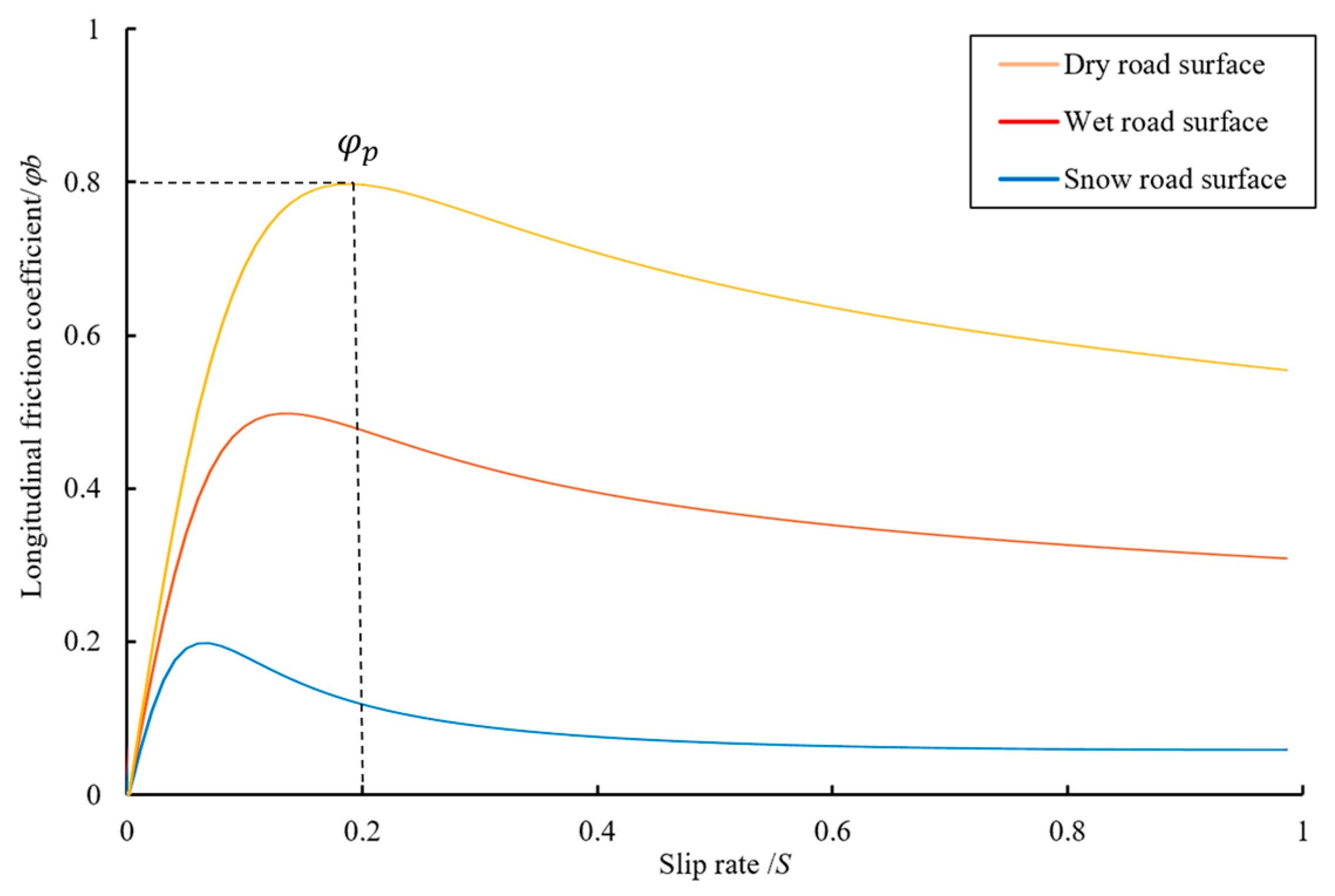
The longitudinal adhesion coefficient ${\phi }_b$ on different road surfaces exhibits a nonlinear relationship with the slip ratio $s$. Consequently, during the braking process, the ground braking force $F_{xb}$ acting on the wheel initially increases with the rise in the slip ratio $s$ until it reaches the maximum adhesion force $F_p$ (corresponding to the peak adhesion coefficient ${\phi }_p$). After reaching this peak, the braking force gradually decreases until the wheel locks up completely.

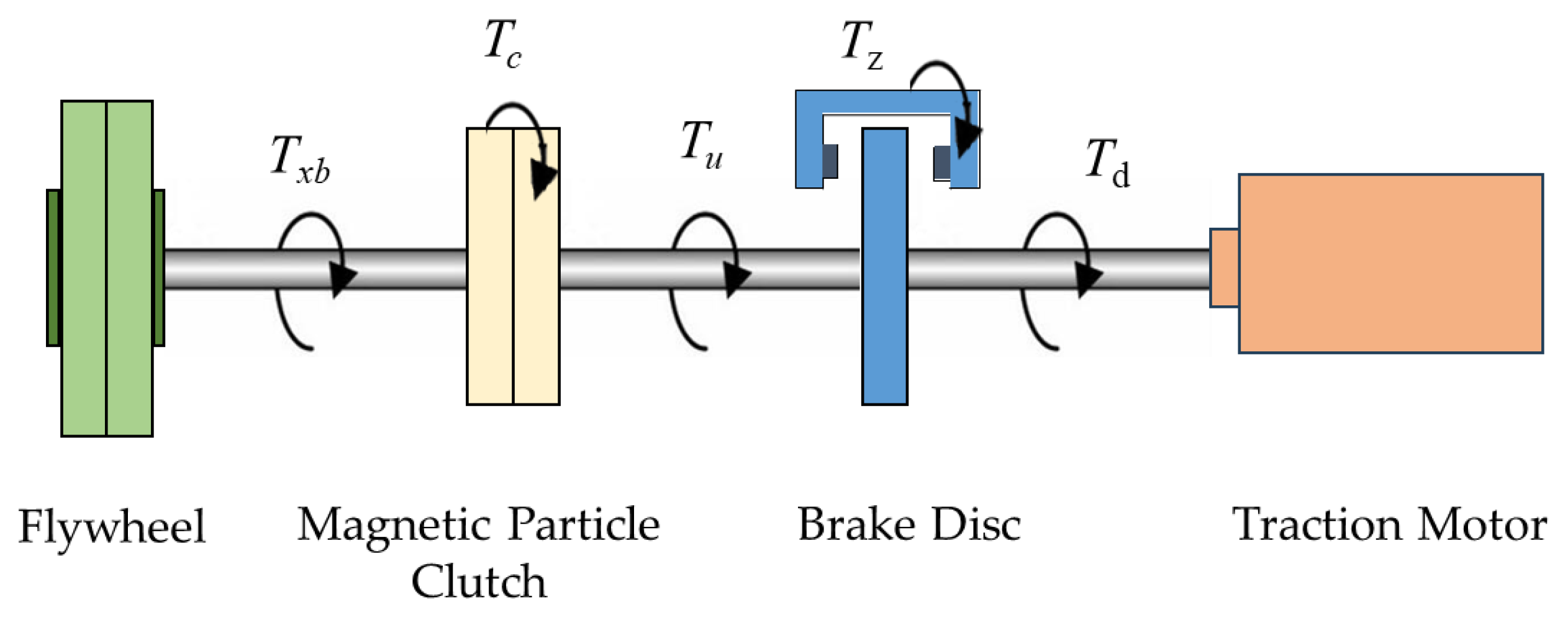
In the context of integrated control experiments, it is essential to account for the ground braking force when transmitting both the braking force and regenerative braking force to the flywheel via the magnetic powder clutch. Figure 6 illustrates a schematic diagram of the torque transmission among the primary components during braking tests conducted on this experimental platform.

In Figure 6, $T_{\mu }$ represents the resultant braking torque (hereafter referred to as the equivalent braking torque), which is the sum of the brake torque $T_z$ and the motor regenerative braking torque $T_d$, expressed as $T_{\mu }=T_z+T_d$. The torque transmitted by the magnetic powder clutch is denoted as $T_c$, while $T_{xb}$ corresponds to the actual braking torque exerted on the flywheel. During the experimental process, the equivalent braking torque $T_{\mu }$ is transmitted to the flywheel through the magnetic powder clutch. When $T_{\mu }$ is less than the maximum transmissible torque $T_{Cmax}$ of the magnetic powder clutch, the clutch operates in a rigidly connected state. Under this condition, the entire equivalent braking torque $T_{\mu }$ is transferred to the flywheel, resulting in flywheel deceleration, i.e., $T_{xb}=T_{\mu }$. However, when $T_{\mu }$ exceeds $T_{Cmax}$, the wheel enters an anti-lock regulation state. In this scenario, the system dynamically adjusts the torque transmitted by the magnetic powder clutch based on the relationship between the longitudinal adhesion force and the slip ratio of the selected road surface, thereby simulating the dynamic variations in ground braking force.

During vehicle braking, the braking force exerted by the ground on the wheels can be expressed as:

$$F_{xb}=G\cdot {\phi }_b$$

(8)

where, $F_{xb}$ is the braking force exerted by the ground on the wheels, $G$ is the total gravitational force of the vehicle, ${\phi }_b$ is the longitudinal adhesion coefficient.

The magic formula tire model, proposed by Pacejka, is capable of accurately fitting experimental data for tires under various operating conditions, including longitudinal force, lateral force, aligning torque, overturning moment, and rolling resistance, among others [36]. This study focuses on the longitudinal force between the tire and the road surface. The relevant expression of the magic formula is as follows:

$$\phi \left(s\right)={\phi }_0+\mathrm{A}sin\left\{\mathrm{B}arctg\left[\mathrm{C}s-\mathrm{D}(\mathrm{C}s-arctg(\mathrm{C}s\left)\right)\right]\right\}$$

(9)

where, ${\phi }_0$ is the adhesion coefficient when the wheel is in pure rolling, typically set to 0 under general conditions, A, B, C and D are undetermined parameters, which are constants related to the road surface, $s$ represents the slip ratio.

By adjusting these parameters, the formula can precisely simulate the adhesion coefficient and slip ratio curves for various road surfaces (Figure 7). The parameters, fitted to experimental data, are given in

Table 2. Parameter Values of Three Typical Road Surfaces.

Parameter Values	A	B	C	D	${\mathit{\phi }}_{\mathit{p}}$	${\mathit{s}}_{\mathit{p}}$
Asphalt road surface	0.8	2.4	5.0	0.96	0.8	0.2
Sand road surface	0.5	2.5	6.5	0.98	0.5	0.15
Snow road surface	0.2	3.0	10	1.01	0.2	0.07

.

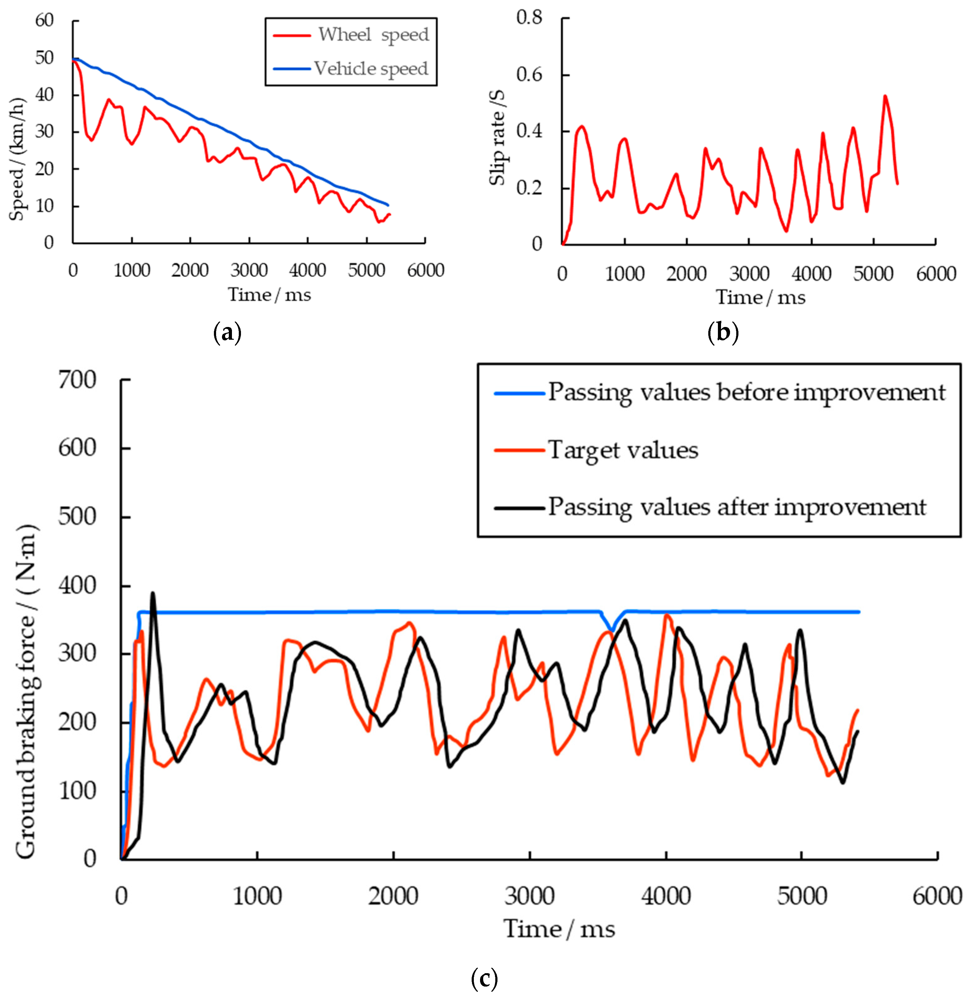
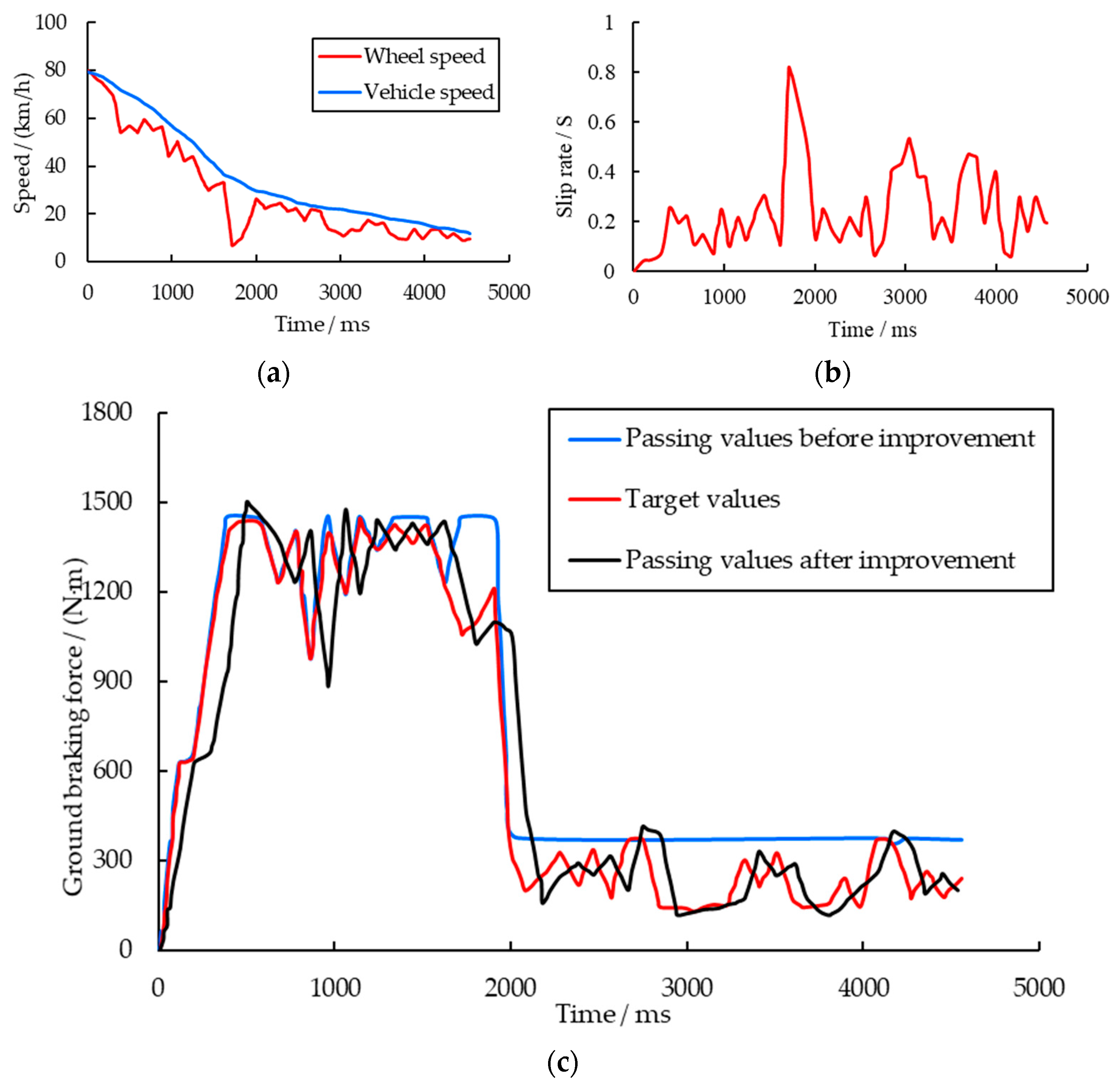
To simulate the changes in ground braking force with respect to the slip ratio during the braking process, the ground braking force simulation controller calculates the slip ratio based on the rotational speed signals of the flywheel and the brake disc. It then determines the longitudinal adhesion coefficient by referencing the selected road surface’s ${\phi }_b$-$s$ curve and the magic formula. Based on the determined longitudinal adhesion coefficient, the system calculates the corresponding ground braking force and converts it into the target torque for the magnetic powder clutch.

The magnetic powder clutch computes the actual braking torque applied to the flywheel using signals from the flywheel torque sensor. The deviation between the measured braking torque and the target torque is used to calculate the required programmable power supply output. The ground braking force simulation controller adjusts the output current of the programmable power supply based on this value, thereby modifying the transmitted torque of the magnetic powder clutch. This process enables precise closed-loop tracking control of the target torque.

4.2. Ground Braking Force Simulation Control Target Torque Selection Strategy

4.2.1. Single-Road Surface Ground Braking Force Simulation Control Strategy

According to braking principles, when the slip ratio $s$ is below the optimal slip ratio, the ground braking force equals the combined force of the brake torque and the motor regenerative braking torque. However, when the slip ratio $s$ exceeds the optimal slip ratio, the ground braking force deviates significantly from this combined force. Therefore, during the control process, if the slip ratio is detected to be below the optimal slip ratio, a constant torque control method is adopted. Conversely, when the slip ratio is detected to exceed the optimal slip ratio $s_p$, a variable target torque control method is employed, expressed as:

$$T_{target}=\left\{\begin{array}{cc}\hfill T_p,& s\le s_p\hfill \\ \hfill T\left(\mathrm{s}\right),& s>s_p\hfill \end{array}\right.$$

(10)

where, $s_p$ is the optimal slip ratio, $T_{target}$ is the target torque of the magnetic powder clutch, $T\left(s\right)$ is the braking torque exerted by the selected road surface on the wheel, $T_p$ is the braking torque generated by the maximum adhesion force on the wheel.

The specific control strategy is illustrated in Figure 8.

4.2.2. Ground Braking Force Simulation Control Strategy for Transitional Road Surfaces

The simulation of ground braking force on transitional road surfaces is divided into two phases: the pre-transition phase (Road Surface A) and the post-transition phase (Road Surface B). Before the road surface transition, the control strategy is identical to that of a single road surface. Specifically, the slip ratio $s$ is compared with the optimal slip ratio $s_{pA}$ of Road Surface A, as follows:

$$T_{target}=\left\{\begin{array}{cc}\hfill T_{pA},& s\le s_{pA}\hfill \\ \hfill T_A\left(s\right),& s>s_{pA}\hfill \end{array}\right.$$

(11)

At the moment of road surface transition, the system determines the target torque for the magnetic powder clutch after the transition based on the slip ratio and the ${\phi }_{\mathrm{b}}$−$s$ curve of Road Surface B. Once the transition is complete, the system continues to monitor the slip ratio and adjusts the target torque according to the operating conditions of Road Surface B, as follows:

$$T_{target}=\left\{\begin{array}{cc}\hfill T_{pB},& s\le s_{pB}\hfill \\ \hfill T_B\left(s\right),& s>s_{pB}\hfill \end{array}\right.$$

(12)

The specific control strategy is illustrated in Figure 9.

While the current control strategy adopts fixed optimal slip ratios (15–20%) for different road conditions, it should be noted that real-world scenarios may exhibit dynamic threshold variations due to factors including but not limited to: (1) tire wear and aging effects, (2) vehicle load distribution changes, (3) road surface heterogeneity, and (4) temperature-dependent friction characteristics.

4.3. Design of the Magnetic Powder Clutch Controller

4.3.1. Parameters of the Magnetic Powder Clutch

The magnetic powder clutch is one of the most critical components of the ground braking force simulation system. Its primary function is to dynamically simulate the ground braking force by adjusting its transmitted torque in real time. The magnitude of the torque transmitted by the magnetic powder clutch can be controlled by regulating its excitation current [37].

As depicted in Figure 10, a CJ-40 type magnetic powder clutch (Nantong Aerospace Electromechanical Automation Co., Ltd., Nantong, China) was selected as the experimental platform. The parameters of this clutch are listed in

Table 3. Related parameters of magnetic powder clutch.

Model	Rated Voltage	Rated Torque	Maximum Speed
CJ-40	12 V	700 N·m	4000 r/min

.

4.3.2. Mathematical Model Analysis of the Magnetic Powder Clutch

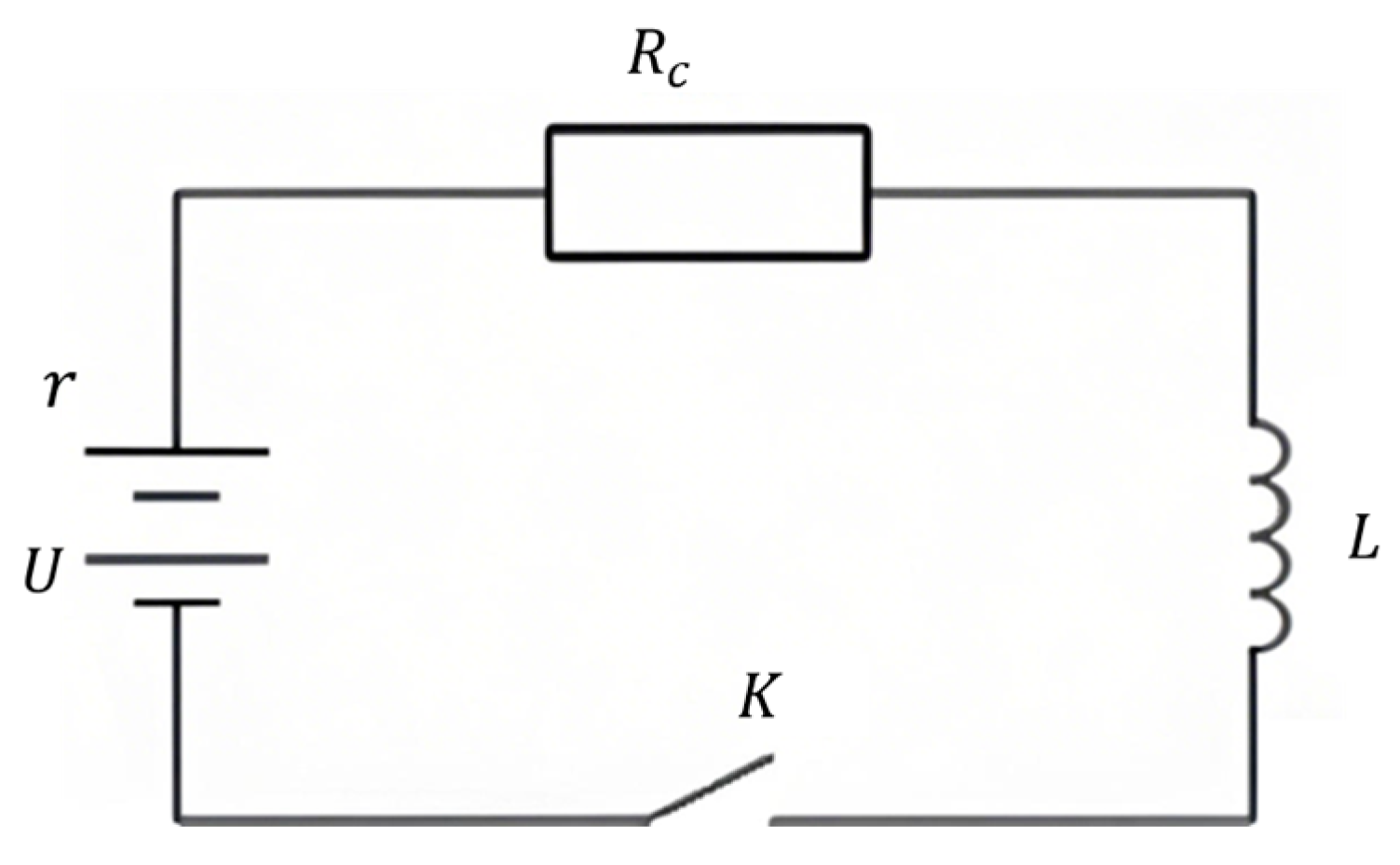
To facilitate quantitative calculations of the excitation current transient process in the magnetic powder clutch, certain simplifications are applied to its characteristics. These simplifications include neglecting the hysteresis effects of magnetic flux and magnetic particles on the circuit during the transition process, as well as variations in the inductance of the excitation coil. The excitation circuit of the magnetic powder clutch can be simplified as shown in Figure 11 [38].

When switch K is closed, a current is generated in the circuit. The voltage balance equation for the circuit is as follows:

$${(R}_L+R_C)·i+L{\displaystyle \frac{di}{dt}}=U-ri$$

(13)

Solving Equation (13) yields the variation pattern of the current in the circuit as follows:

$$i=I(1-e^{-t/T_i})$$

(14)

The current time constant $T_i=L/R$, where L is the magnetic powder clutch coil inductance [H] and $R$ = $R_L+R_C+r$, is the total excitation circuit resistance [Ω] (including excitation coil resistance $R_L$, series resistance $R_C$, and power supply internal resistance $r$), with steady-state current $I=U/R$ determined by excitation voltage U [V].

Building on the transient current analysis in Equation (14), which reveals the nonlinear hysteresis characteristics of the excitation circuit, we now examine the torque transmission behavior. The static torque-current relationship demonstrates dual-phase nonlinearity. To establish a tractable dynamic model while preserving essential physical characteristics, we implement the following simplifications:

• Exclusion of no-load torque $M_0$
• Linearization of dead-zone effects
• Hysteresis loop approximation

This leads to the piecewise linearized torque model:

$$M=K_m·i (m\in \mathrm{1,2},3,\dots \dots )$$

(15)

The coefficient $K_m$, which represents the torque-current relationship, is determined by the specific current-torque characteristic curve of the magnetic particle clutch. This parameter can be obtained through experimental calibration or manufacturer specifications, taking into account the operating conditions and material properties of the magnetic particles.

While the linear approximation (Equation (15)) provides computational simplicity, it is important to acknowledge three inherent nonlinear characteristics of magnetic powder clutches:

(a)

Hysteresis effects in magnetization-demagnetization cycles (up to 8–12% torque variation observed in preliminary tests)

(b)

Non-constant Km values across operating regions (typically 15–20% higher in weak excitation vs. saturation regions)

(c)

Temperature-dependent time delay $T_d$ (experimental data shows ±7% variation within 20–80 °C range)

The governing equations can be derived by reorganizing Equations (13) and (15), yielding the following system:

$$\left\{\begin{array}{c}I=U/R\\ {\displaystyle \frac{di}{dt}}={\displaystyle \frac{I-i}{T_i}}\\ M=K_m·i\end{array}\right.$$

(16)

The electromechanical dynamics of the magnetic particle clutch system are described by the following fundamental relationships:

$$\left\{\begin{array}{c}\mathrm{Torque}-\mathrm{Current} \mathrm{Law}:M_t=K_m· i\left(t\right)\\ \mathrm{Coil} \mathrm{Circuit} \mathrm{Equation}: U\left(t\right)=Ri\left(t\right)+L{\displaystyle \frac{di\left(t\right)}{dt}}\end{array}\right.$$

(17)

Under zero initial conditions, the Laplace transform of the circuit equation yields:

$$U\left(S\right)=\left(R+LS\right)I\left(S\right)⟹I\left(S\right)={\displaystyle \frac{\frac{1}{R}}{T_{i}S+1}}U(S), T_i={\displaystyle \frac{L}{R}}$$

(18)

Here, $T_i=L/R$ represents the electrical time constant governing the transient response of the excitation current.

Substituting I(S) into the torque equation M(S) = $K_m$I(S), the initial transfer function is derived as:

$$G_z\left(S\right)={\displaystyle \frac{M\left(S\right)}{U\left(S\right)}}={\displaystyle \frac{K_m\frac{1}{R}}{T_{i}S+1}}={\displaystyle \frac{K_z}{T_{i}S+1}}$$

(19)

where, $K_z=K_m/R$ represents the overall system gain of the excitation coil circuit in the magnetic particle clutch, with units of Nm/V.

To account for the practical torque hysteresis caused by magnetic particle magnetization lag and mechanical shear delay, a pure time delay term $e^{-T_{d}S}$ is introduced:

$$G_Z\left(S\right)={\displaystyle \frac{K_z}{T_{i}S+1}}{e}^{-T_{d}S}$$

(20)

where, $T_d$ represents the time delay constant of the magnetic particle clutch, characterizing the hysteresis effect between the excitation current and the output torque.

Tests were conducted on the response characteristics of the magnetic particle clutch on the test platform, with the parameters listed in

Table 4. Response characteristic parameter values of magnetic powder clutch.

State	Time Parameter	Parameter Value/s
Power-on	Current time constant $T_i$	0.05
	Torque time constant $T_t$	0.07
	Torque dead time $T_d$	0.01

.

The first-order model with time delay (Equation (20)) captures dominant dynamics but has inherent limitations. Our experimental validation (see Appendix A for detailed test conditions) showed that when the target (steady-state) output torque exceeds 30% of the rated torque, the step response prediction fidelity reaches 92.3%; this decreases to 85.7% when the target torque is below 15% rated torque due to nonlinear effects. These variations are mitigated by the fuzzy adaptive controller’s compensation capability.

4.3.3. The Design of a Fuzzy Adaptive PID Controller

As shown in Equation (20), the magnetic particle clutch exhibits first-order inertial behavior with hysteresis, making it inherently a Type 0 system. Due to these characteristics, conventional PID control fails to provide satisfactory performance in terms of response speed and stability. To achieve precise torque transmission control—ensuring rapid response, stable operation, and compliance with experimental requirements—a dedicated controller must be designed.

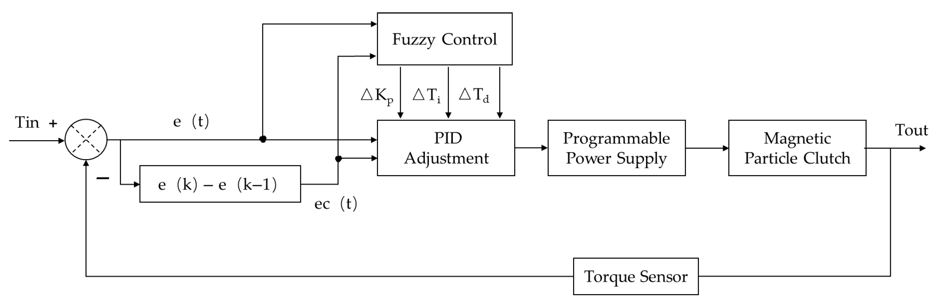
This development is especially critical for the electric vehicle ABS and RBS integrated control test platform, where accurate simulation of ground braking forces is essential for reliable system evaluation. To address these challenges, a fuzzy adaptive PID controller is implemented using a two-dimensional control structure (Figure 12). This architecture features:

Input Variables:

• $e\left(t\right)=M_{ref}\left(t\right)-M_{actual}\left(t\right)$: torque error
  where, $M_{ref}$ = reference torque, $M_{actual}$ = measured transmitted torque.
• $ec(t)={\displaystyle \frac{\mathrm{d}e\left(t\right)}{\mathrm{d}t}}$: rate of change of torque error

Output Variables:

• $∆K_{\mathrm{p}}$: incremental adjustment of proportional gain;
• $∆T_{\mathrm{i}}$: incremental adjustment of integral time constant;
• $∆T_{\mathrm{d}}$: incremental adjustment of derivative time constant.

The online tuning mechanism continuously adjusts the PID parameters based on the fuzzy logic rules, which map the input variables ($e,ec$) to the output increments ($∆K_p, ∆T_i, ∆T_d$). This adaptive approach enables the controller to maintain optimal performance across various operating conditions.

The scaling factors $K_e$ and $K_{ec}$, which normalize the input variables to the fuzzy controller, are defined by Equations (21) and (22).

$$K_e={\displaystyle \frac{n_e}{e_{max}}}$$

(21)

$$K_{ec}={\displaystyle \frac{n_{ec}}{{ec}_{max}}}$$

(22)

where $K_e$ and $K_{ec}$ denote the scaling factors for error and error rate respectively, $n_e$ and $n_{ec}$ represent their quantization levels, while $e_{max}$ and ${ec}_{max}$ indicate the maximum expected values of error and error rate.

The output variables, which are initially in the fuzzy domain, require conversion to the basic domain of control quantities through appropriate scaling factors. $K_{{∆K}_p}, K_{{∆T}_i}, K_{{∆T}_d}$ are defined as the scaling factors of ${∆K}_p$, ${∆T}_i$, ${∆T}_d$, respectively. These scaling factors are calculated by Equations (23)–(25).

$$K_{{∆K}_p}={\displaystyle \frac{{{∆K}_p}_{max}}{n_{{∆K}_p}}}$$

(23)

$$K_{{∆T}_i}={\displaystyle \frac{{{∆T}_i}_{max}}{n_{{∆T}_i}}}$$

(24)

$$K_{{∆T}_d}={\displaystyle \frac{{{∆T}_d}_{max}}{n_{{∆T}_d}}}$$

(25)

where, ${{∆K}_p}_{max}, {{∆T}_i}_{max}, {{∆T}_d}_{max}$ indicate the maximum expected values of the output variables, $n_{{∆K}_p},n_{{∆T}_i},n_{{∆T}_d}$ represent the number of quantization levels for the output variables, respectively.

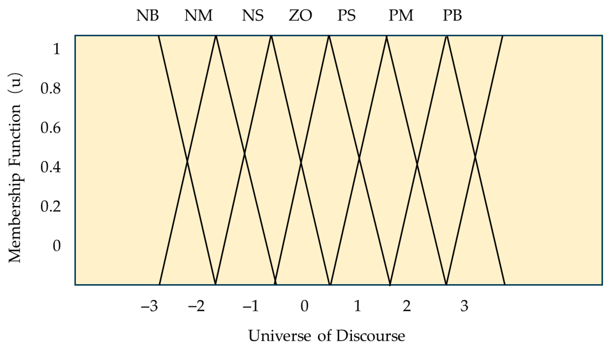
After determining the input and output variables, it is essential to define the fuzzy subsets for all variables based on the research object and control requirements. The number of linguistic values used to describe fuzzy variables should be chosen according to practical needs. Generally, a greater number of linguistic values can improve control performance. However, an excessive number may increase the complexity of the algorithm, potentially degrading control effectiveness. In this study, considering the control requirements of the ground braking force simulation system, seven linguistic values are selected to describe the variables [39].

The fuzzy set domain for both input and output variables is defined as: $\left\{-n,-n+1,\dots ,0,\dots ,n-1,n\right\}$. The value of n can be determined based on empirical knowledge or experimental conditions, and it may vary for different variables. In this study, considering the specific control requirements of the system, a combination of half-trapezoidal, triangular, and half-trapezoidal functions is selected as the membership functions for the input and output variables of the fuzzy control section, as illustrated in Figure 13.

The digital implementation of the PID algorithm requires discretization of the continuous-time controller due to the sampled nature of feedback data. The discrete-time PID control law is given by Equation (26).

The continuous-time PID controller requires discretization for digital implementation. Using backward difference approximation with sampling period $T_s$, the discrete control law becomes:

$$\mathrm{U}\left(\mathrm{n}\right)=K_p\left[e_n+{\displaystyle \frac{T_s}{T_i}}\sum _{j=1}^n{e}_j+{\displaystyle \frac{T_d}{T_s}}(e_n-e_{n-1})\right]$$

(26)

where $\mathrm{U}\left(\mathrm{n}\right)$ denotes the control output at the nth sampling instant, $K_p$ is the proportional gain, $T_i$, and $T_d$ represent the integral and derivative time constants, respectively, and $T_s$ is the sampling period. The term $e_n$ corresponds to the error at the $n^{th}$ sampling instant, while $e_{n-1}$ refers to the error at the previous ${(n-1)}^{th}$ sampling instant.

The fuzzy-adaptive mechanism dynamically adjusts these parameters through:

$$\left\{\begin{array}{c}{K}_p=K_{p0}+{∆K}_p\\ T_i=T_{i0}+∆T_i\\ T_d=T_{d0}+∆T_d\end{array}\right.$$

(27)

where, $K_{p0},T_{i0},T_{d0}$ indicate the initial PID parameters (proportional gain, integral time constant, and derivative time constant, respectively), ${∆K}_p, ∆T_i, ∆T_d$ represent incremental adjustments provided by the fuzzy controller.

The fuzzy rule base specifically incorporates compensation mechanisms for:

• Weak-excitation region: 25% heavier weighting on derivative action
• Saturation region: 15% reduced proportional gain.
• Hysteresis compensation: Additional 50 ms lead time in ∆Td adjustment

The fuzzy control rule tables for ${∆K}_p$, $∆T_i$ and $∆T_d$ are established separately and presented in

Table 5. $∆K_p$’s fuzzy control rule table.

$\mathit{e}$	$\mathit{e}\mathit{c}$
	NB	NM	NS	ZO	PS	PM	PB
NB	PB	PB	PM	PM	PS	ZO	ZO
NM	PB	PB	PM	PS	PS	ZO	NS
NS	PM	PM	PM	PS	ZO	NS	NS
ZO	PM	PM	PS	ZO	NS	NM	NM
PS	PS	PS	ZO	NS	NS	NM	NM
PM	PS	ZO	NS	NM	NM	NM	NB
PB	ZO	ZO	NM	NM	NM	NB	NB

,

Table 6. $∆T_i$’s fuzzy control rule table.

$\mathit{e}$	$\mathit{e}\mathit{c}$
	NB	NM	NS	ZO	PS	PM	PB
NB	NB	NB	NM	NM	NS	ZO	ZO
NM	NB	NB	NM	NS	NS	ZO	ZO
NS	NB	NM	NS	NS	ZO	PS	PS
ZO	NM	NM	NS	ZO	PS	PM	PM
PS	NM	NS	ZO	PS	PS	PM	PB
PM	ZO	ZO	PS	PS	PM	PB	PB
PB	ZO	ZO	PS	PM	PM	PB	PB

and

Table 7. $∆T_d$’s fuzzy control rule table.

$\mathit{e}$	$\mathit{e}\mathit{c}$
	NB	NM	NS	ZO	PS	PM	PB
NB	PS	NS	NB	NB	NB	NM	PS
NM	PS	NS	NB	NM	NM	NS	ZO
NS	ZO	NS	NM	NM	NS	NS	ZO
ZO	ZO	NS	NS	NS	NS	NS	ZO
PS	ZO	ZO	ZO	ZO	ZO	ZO	ZO
PM	PB	PS	PS	PS	PS	PS	PB
PB	PB	PM	PM	PM	PS	PS	PB

, respectively.

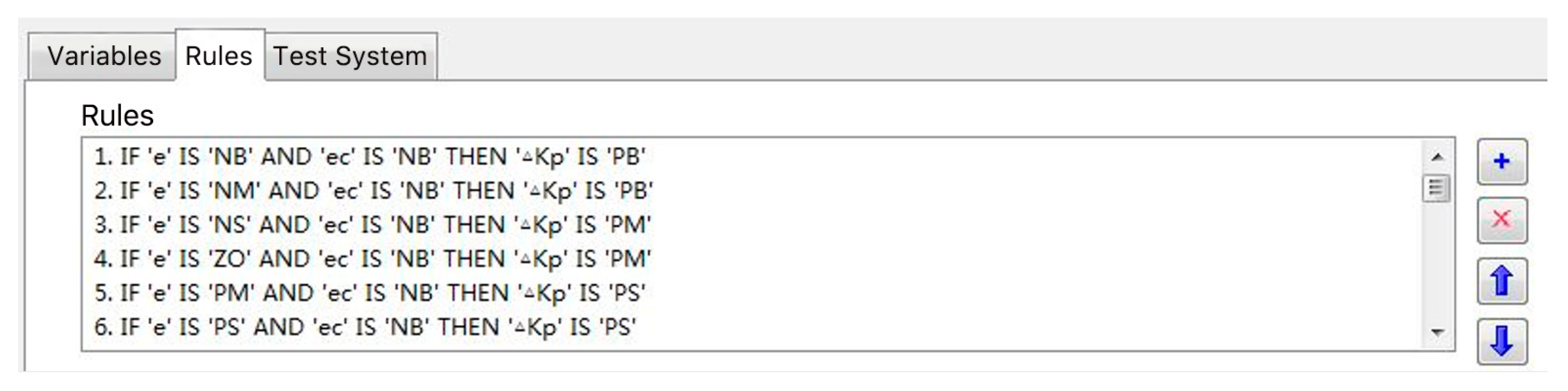
All 49 fuzzy control rules mentioned above have been implemented in the computer program, with the corresponding interface displayed in Figure 14.

Considering the requirements of braking force simulation control, this study adopts the Mamdani fuzzy inference method. The established fuzzy control system comprises 49 rules, with each fuzzy control relation denoted as ${\mathrm{R}}_{\mathrm{i}}$. These fuzzy relations are connected by the logical “OR” operator. Consequently, the overall fuzzy relation of the control rules can be expressed as:

$$R=\bigcup _{i=1}^{49}{R}_i$$

(28)

Let $\mathrm{E}$ be the linguistic deviation variable and EC be the deviation change rate as the inputs of the fuzzy controller. Based on the overall fuzzy relation $R$ derived from Equation (28), the output control variable can be obtained as:

$$C={\left(E\times EC\right)}^T ° R$$

(29)

where, ${\left(E\times EC\right)}^T$ represents the transpose of the fuzzy relation matrix.

The defuzzification process employs the weighted average method. With seven elements in the output domain, each denoted as $x_i$, and the membership degree of the output fuzzy set as ${\mu }_c\left(x_i\right)$, the final decision value using the weighted average method is given by:

$$C={\displaystyle \frac{\sum _{i=1}^7{x}_i{\mu }_C\left(x_i\right)}{{\sum }_{i=1}^7{\mu }_C\left(x_i\right)}}$$

(30)

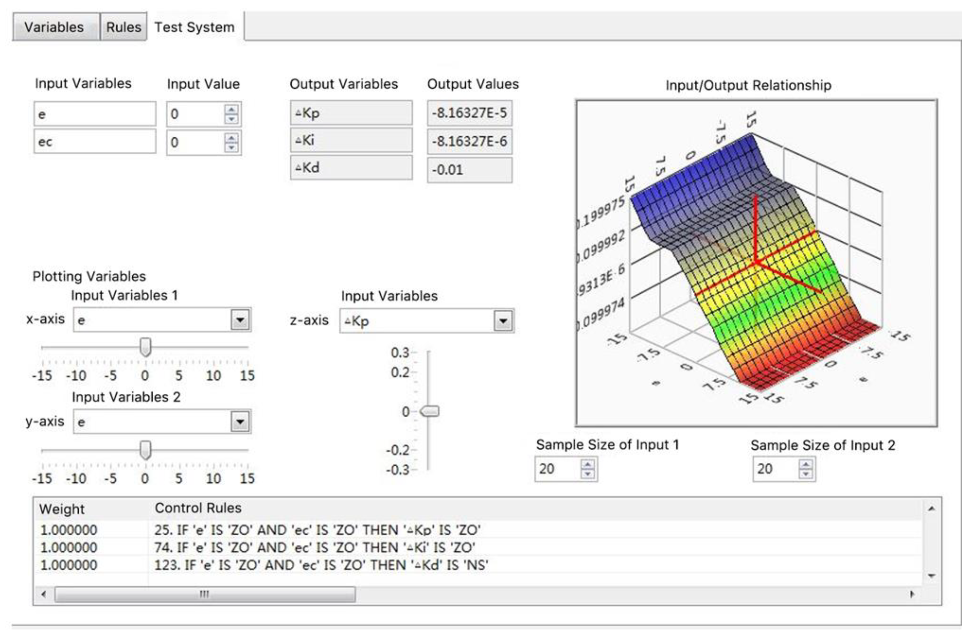
Upon completing these procedures, the designed fuzzy adaptive PID controller can be observed in the fuzzy system designer. This includes the input-output correspondence under fuzzy rules and the surface plots representing the relationship between output and input variables of the fuzzy controller. The observation interface is illustrated in Figure 15.

The key parameters of the fuzzy adaptive PID controller were determined through theoretical analysis and optimization tuning according to the system control requirements, as presented in

Table 8. Parameters of the Fuzzy Adaptive PID Controller.

Parameter Category	Parameter Name	Symbol	Value/Range	Remarks
Basic Parameters	Control Cycle	$T_s$	30 ms	Sampling period
Input Variables	Error	$\mathrm{e}$	[−300, +300]	Universe of discourse
	Error Rate	$\mathrm{e}\mathrm{c}$	/	/
	Error Scaling Factor	$K_e$	0.01	/
	Error Rate Scaling Factor	$K_{ec}$	0.05	/
Output Variables	Proportional Gain Adjustment	${∆K}_p$	[−0.0006, +0.0006]	Tuning output
	Integral Time Adjustment	${∆T}_i$	[−0.00003, +0.00003]	Tuning output
	Derivative Time Adjustment	${∆T}_d$	[−0.000015, +0.000015]	Tuning output
	${∆K}_p$ Scaling Factor	$K_{{∆K}_p}$	$2\times {10}^{-4}$	/
	${∆T}_i$ Scaling Factor	$K_{{∆T}_i}$	$1\times {10}^{-5}$	/
	${∆T}_d$ Scaling Factor	$K_{{∆T}_d}$	$5\times {10}^{-6}$	/
Linguistic Variables	Term Set	/	$\left\{-3,-2,-1, 0, 1, 2, 3\right\}$	/

.

Through systematic parameter space exploration and gradient-based optimization, the globally optimal PID parameters were identified as:

• Proportional gain: $K_p=4.00\times {10}^{-3}$;
• Integral time constant: $T_i=8.13\times {10}^{-3}s$;
• Derivative time constant: $T_d=1.80\times {10}^{-3}s$.

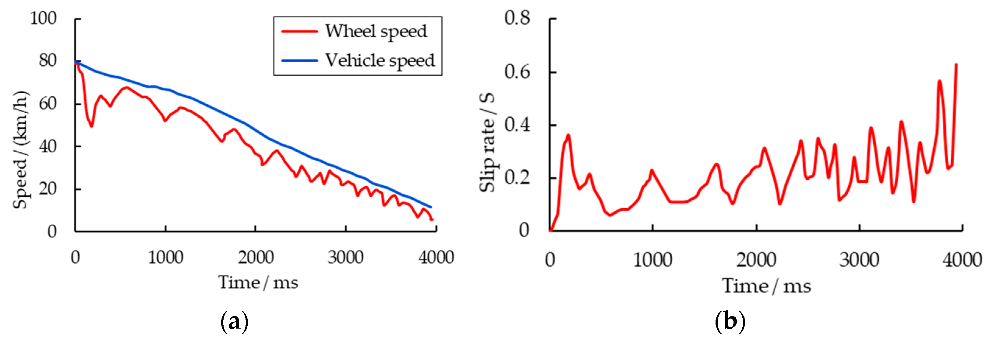
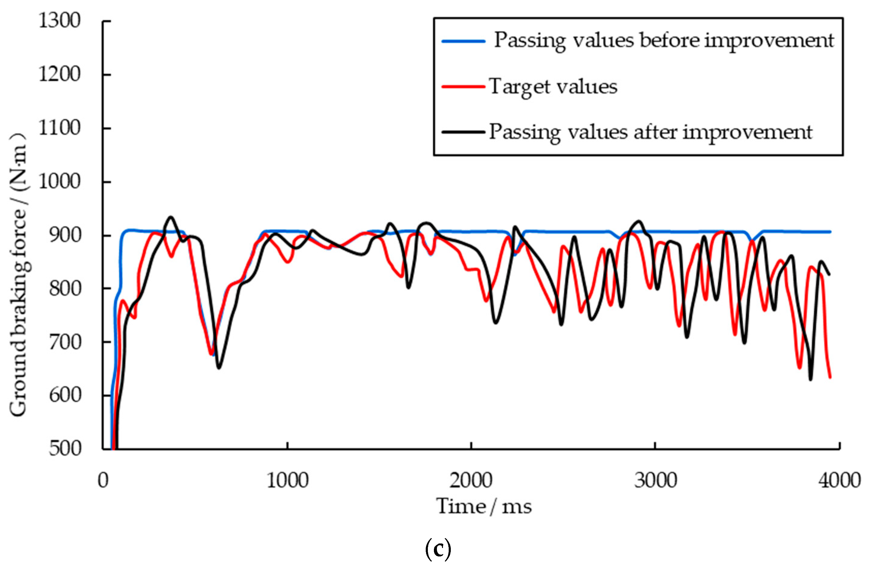
The designed magnetic particle controller underwent parameter tuning and optimization, with experimental validation confirming the feasibility of the proposed control algorithm (Figure 16). Quantitative comparisons with a conventional PID controller reveal that the fuzzy adaptive PID controller achieves superior performance: (1) overshoot is reduced from 18.7% to 8.5%, (2) rise time is shortened from 88.7 $\mathrm{m}\mathrm{s}$ to 40.9 $\mathrm{m}\mathrm{s}$, and (3) settling time decreases from 687.1 ms to 458.1 ms. (The control parameters for the conventional PID controller are given in time-constant form as: $K_p=8.0\times {10}^{-3}$, $T_i=4.1\times {10}^{-3}s$; $T_d=2.7\times {10}^{-3}s$).

5. Experimental Results

5.1. Experimental Protocol

The experimental procedure initiates with the activation of the drive motor, applying appropriate excitation current to the magnetic particle clutch, which synchronously rotates the flywheel. When the flywheel reaches the initial braking test velocity, the integrated control platform controller allocates the braking torque according to the braking intensity requirements and force distribution strategy, resulting in gradual flywheel deceleration. The ground braking force simulation controller continuously acquires sensor signals to regulate the excitation current of the magnetic particle clutch, thereby modulating its transmission torque. The experiment concludes when the flywheel speed decreases to the predetermined termination threshold.

5.2. Single-Surface Testing

Experimental investigations were conducted on three representative road surfaces: asphalt, sand, and snow. To ensure sufficient data acquisition:

For asphalt and sand surfaces with higher adhesion coefficients, the initial vehicle speed was set at 80$\mathrm{k}\mathrm{m}/\mathrm{h}$. For snow-covered surfaces with lower adhesion coefficients, the initial speed was set at 50 $\mathrm{k}\mathrm{m}/\mathrm{h}$. All single-surface tests were terminated when the vehicle speed decreased to 10 $\mathrm{k}\mathrm{m}/\mathrm{h}$. The experimental results are presented in Figure 17, Figure 18, and Figure 19, respectively.

To evaluate system improvement effectiveness, the ground braking force variation curves were compared with baseline measurements. The pre-improvement transmission values refer to the ground braking force magnitude simulated by applying a constant current corresponding to the maximum adhesion force of the selected road surface model, while neglecting variations in tire-road adhesion force during the experiment.

5.3. Transition Surface Testing

5.3.1. Asphalt to Snow Surface Transition

The road surface model was configured to simulate a transition from asphalt to a snow-covered surface. The experimental parameters were set as follows:

• Initial road surface: Asphalt;
• Transition speed: 30 $\mathrm{k}\mathrm{m}/\mathrm{h}$ (from initial speed of 80 $\mathrm{k}\mathrm{m}/\mathrm{h}$);
• Termination condition: Vehicle speed decreases to 10 $\mathrm{k}\mathrm{m}/\mathrm{h}$.

The experimental results are presented in Figure 20, which illustrates the system response during the surface transition. This testing scenario evaluates the controller’s adaptability to abrupt changes in road adhesion characteristics, particularly from high-adhesion asphalt to low-adhesion snow surface conditions.

5.3.2. Snow to Asphalt Surface Transition

The experimental configuration simulated a road surface transition from snow-covered to asphalt conditions, with the following parameters:

• Initial road surface: Snow;
• Transition speed: 50 km/h (from initial speed of 80 $\mathrm{k}\mathrm{m}/\mathrm{h}$);
• Test termination: Vehicle speed decreases to 10 $\mathrm{k}\mathrm{m}/\mathrm{h}$;

Figure 21 presents the experimental results, demonstrating the system’s performance during this adhesion transition. This test scenario specifically evaluates the controller’s response capability when transitioning from low-adhesion (snow) to high-adhesion (asphalt) road conditions, which represents a critical test case for adaptive braking systems.

Beyond the core performance metrics, the system’s reliability was rigorously evaluated through accelerated stress testing. Three critical aspects were examined: (a) cyclic durability under extreme μ-transitions, (b) thermal operating margins, and (c) long-term stability. Key findings include:

Cyclic durability: 500 asphalt-to-snow transitions at 25 °C showed stable torque output (mean ± SD: 298 ± 12 $\mathrm{N}·\mathrm{m}$, CV = 3.0%), with post-test inspection confirming no magnetic particle agglomeration.

Thermal robustness: At −10 °C/50 °C extremes, the maximum tracking error increased to 4.1% (vs. 2.3% at 25 °C), still within 5% tolerance.

Aging simulation: Continuous 48-h operation at 1.5 A excitation caused only 1.8% gain drift.

5.4. Field Test Implications and System Robustness Analysis

While bench testing provides controlled validation conditions, the system’s real-world applicability requires further evaluation of three critical aspects: vibration immunity, environmental adaptability, and road surface stochasticity.

5.4.1. Vibration Effects Mitigation

Road-induced vibrations in the 2–20 Hz range are expected to have limited impact on torque transmission stability, based on prior studies of similar MPC architectures [40]. The fuzzy-PID controller’s 100 Hz sampling rate exceeds the Nyquist frequency for dominant vibration modes, theoretically enabling effective noise suppression.

5.4.2. Environmental Adaptability

Through dynamic adjustment of the $\phi -s$ mapping relationship, the bench testing platform effectively reproduces both low-adhesion conditions (e.g., snowy roads) and high-adhesion conditions (e.g., dry asphalt), thereby covering the full spectrum of typical weather-induced friction variations. Building upon this capability, the fuzzy-PID controller demonstrates exceptional robustness by maintaining stable torque tracking even during abrupt $\phi$ changes—a critical feature that accurately mimics sudden weather transitions such as rainfall during braking.

Expanding on these results, the system’s rapid response to $\phi -s$ transitions (particularly in challenging sequences like snow→asphalt scenarios) provides compelling evidence of its ability to handle complex, weather-dependent road conditions. Importantly, when compared to conventional real-vehicle testing, this bench-based approach offers distinct advantages: it enables highly repeatable and precisely controllable weather scenario simulations while completely eliminating the unpredictability and logistical challenges associated with actual climate conditions.

This integrated validation methodology therefore bridges the gap between laboratory testing and real-world weather variability, offering researchers a practical tool for comprehensive ABS/RBS development across diverse environmental conditions.

5.4.3. Road Surface Stochasticity

Although bench testing cannot fully replicate road irregularity issues encountered in complete road tests, the proposed fuzzy adaptive PID controller achieves equivalent robustness validation through dynamic $\phi -s$ mapping:

• In both asphalt-to-snow and snow-to-asphalt transition tests, the system demonstrates rapid braking torque adjustment (transition time < 0.1 s, overshoot < 5%), accurately reproducing actual road adhesion transition characteristics.
• Bidirectional $\phi$ transition tests (low→high/high→low) confirm the controller maintains stable output, providing a dynamic verification platform for ABS/RBS strategies that operate independently of mechanical vibration simulation.

6. Discussion

Through systematic experimentation using the ABS/RBS integrated control platform, three key performance dimensions have been quantitatively analyzed: (1) slip rate dynamic response, (2) system tracking accuracy, and (3) ITAE performance metrics. This comprehensive evaluation not only verifies the system’s design objectives but also provides fundamental insights into the hybrid braking dynamics under complex road conditions.

6.1. Slip Rate Dynamics and Control Necessity

The experimental results demonstrate that under integrated ABS-RBS control, the wheel slip ratio exhibits dynamic fluctuations across different road surfaces, with values predominantly exceeding the optimal slip threshold (typically 15–20% for conventional road conditions). As evidenced by Figure 17b, Figure 18b and Figure 19b, asphalt and sandy surfaces maintain moderate slip variability (${\sigma }_{asphalt}$ = 8.2%, ${\sigma }_{sandy}$ = 11.5%), while a pronounced transient instability emerges during asphalt-to-snow transition scenarios (Figure 20b), where the slip ratio oscillates violently with peak deviations reaching 34.7% ($\Delta t$ = 0.8 s). These observations highlight the critical need for real-time adjustment of ground braking forces based on slip ratio dynamics, particularly under rapidly varying road friction conditions.

6.2. System Tracking Performance

The coefficient of determination (R²) between measured and target ground braking forces was quantitatively evaluated across all test scenarios, with detailed results presented in

Table 9. Coefficient of Determination (R²) between Measured and Target Ground Braking Forces for Different Road Surface Tests.

Test Scenario	Road Surface Condition	Coefficient of Determination (R2)	Remark
Single-surface Tests
1	Dry Asphalt	0.942	High-adhesion surface
2	Loose Sand	0.926	Medium-adhesion surface
3	Compacted Snow	0.918	Low-adhesion surface
Transition-surface Tests
4	Asphalt-to-Snow	0.912	High-to-low adhesion
5	Snow-to-Asphalt	0.908	Low-to-high adhesion

Notes: All tests were conducted under controlled environmental conditions (temperature: 20 ± 2 °C, humidity: 50 ± 5% RH); The target values were calculated based on the theoretical model of ground braking force; The coefficient of determination was calculated using least squares method; Each test was repeated 10 times to ensure statistical significance.

.

These results indicate excellent tracking performance of the ground braking force simulation control system, confirming that the designed magnetic particle clutch controller meets the requirements for both single-surface and transition-surface testing.

6.3. ITAE Performance Metrics

The coefficient of determination (R²) between measured and target ground braking forces for three single-surface conditions (asphalt, sand, and snow) and two transition-surface conditions (asphalt-to-snow and snow-to-asphalt) was calculated and presented in

Table 10. Coefficient of Determination (R²) for Ground Braking Force Measurement.

Surface Condition	Pre-Improvement J (ITAE)	Post-Improvement J (ITAE)
Asphalt	183.500	152.615
Sand	232.354	192.615
Snow	500.969	236.470
Asphalt-to-snow	139.345	119.916
Snow-to-asphalt	158.148	144.981

.

The significantly lower ITAE values of the improved system demonstrate that the ground braking force simulation based on slip rate variations more accurately reflects the actual ground braking force. The enhanced control system substantially improves the simulation accuracy of ground braking force in ABS and RBS integrated control experiments.

6.4. System Response Characteristics

The improved system demonstrated consistently superior performance in ground braking force control compared to the pre-improvement baseline, achieving more precise target value tracking with significantly reduced overshoot and oscillation while exhibiting enhanced dynamic responsiveness during transient conditions. The only exception was a slight lag in measured ground braking force during the instant of surface transition in transition-surface braking scenarios.

7. Conclusions and Future Perspectives

This study fundamentally advances the testing and control paradigms for integrated ABS/RBS systems in electric vehicles by directly addressing the two fundamental limitations plaguing traditional bench testing systems identified in the literature:

• Overcoming Static Adhesion Modeling: Traditional approaches rely on static adhesion models (fixed $\phi -s$ curves), which are inherently incapable of replicating the critical real-time dynamics of slip ratio evolution during braking events, especially under transient road conditions.
• Eliminating Open-Loop Control Deficiencies: Conventional systems often employ open-loop control for magnetic powder clutches (MPCs), leading to unacceptably high torque tracking errors during adhesion coefficient transitions ($\phi$-transitions), severely limiting simulation fidelity.

Our core contributions, achieved through the development of a novel MPC-based dynamic simulation system featuring the designed fuzzy adaptive PID controller, are:

(1)

Precise Dynamic Simulation of Ground Braking Force: We establish a closed-loop, high-fidelity simulation capability that accurately replicates the dynamic variation of ground braking force with slip ratio in real-time. This directly solves Limitation #1 by moving beyond static $\phi -s$ curves and enabling faithful simulation of complex slip dynamics under both uniform and transient road surfaces (e.g., asphalt-to-snow transitions).

(2)

High-Accuracy Torque Tracking for MPCs: We validate the superiority of fuzzy adaptive PID control in managing the dual nonlinearities inherent in MPC operation. This controller achieves precise torque regulation, effectively mitigating the large tracking errors associated with open-loop MPC control (Limitation #2). The result is robust performance during critical adhesion transitions, a capability absent in traditional bench setups.

(3)

A Novel High-Fidelity Bench-Testing Methodology: Building upon contributions (1) and (2), we establish an integrated testing paradigm that overcomes the transient simulation limitations of conventional approaches. This methodology provides a controlled, repeatable, and realistic environment for evaluating integrated ABS/RBS performance under the most challenging conditions.

Key findings and experimental validation confirm:

• The proposed fuzzy adaptive PID algorithm effectively addresses road surface nonlinearity: The dynamic coupling between slip ratio and adhesion coefficient manifests as nonlinear torque-slip dynamics during road transitions. This is managed through our core adaptive control strategy featuring real-time $\phi -s$ based torque regulation and threshold switching between Tp and T(s). Experimental results demonstrate the robustness of the proposed scheme, achieving performance improvements ranging from 8.3% to 52.8% in the ITAE metric. This indicates a significant enhancement in the dynamic response of the designed ground braking force dynamic simulation system. The adopted control algorithm maintains effectiveness under extreme conditions, particularly on snow surfaces. Although the ITAE improvement is more modest in transitional scenarios (Asphalt-to-Snow/Snow-to-Asphalt), it still reveals potential for further optimization.
• The developed high-precision braking force model achieves remarkable accuracy (R² > 0.9). It excels… critically, in dynamic tracking during transient road scenarios involving abrupt slip ratio changes ($s$ jumps between 0.2–0.8), validated under challenging cross-surface conditions including μ-jumps (e.g., asphalt-to-snow) Our integrated testing approach with adaptive $T_p/T\left(S\right)$ switching achieved 91–94% fidelity in reproducing these critical adhesion transitions, demonstrating the model’s capability.
• The integrated bench-testing platform and methodology establish a pioneering benchmark for validating EV composite braking systems. Therefore, we propose formally incorporating this methodology and its core control strategies into the T/CSAE 167-2020 standard [41] as a new “road adaptation” clause. This addition will equip the standard with advanced testing capabilities that authentically replicate real-world complex conditions—particularly transient $\phi$-variation scenarios—thus enabling more comprehensive evaluation of holistic system performance and safety boundaries in EV composite braking.

Future Perspectives: While the current platform offers significant advantages over real-road testing for slip control and extreme-condition characterization, the following limitations present key avenues for future research to enhance fidelity and scalability:

• Enhanced Dynamic Fidelity: The absence of 6-DOF vehicle dynamics (e.g., suspension and body oscillations) limits simulation realism. Future work will integrate the platform with a multi-axis vibration system to replicate these critical inertial effects.

Mitigation of Clutch Nonlinearities: The phase lag and hysteresis induced by the magnetic particle clutch introduce control challenges. This will be tackled through the development and implementation of real-time delay estimation coupled with adaptive hysteresis compensation algorithms.

Incorporation of Environmental Factors: The influence of temperature and wear on the tire-road interface is not yet simulated. Future validation will combine thermal-wear modeling with environmental chamber testing to replicate these crucial degradation effects.

Validation of Stochastic Inputs: The simulation of road roughness and transient impacts requires further correlation. Comprehensive real-vehicle testing across varied terrains (e.g., cobblestone, washboard, potholes) will be conducted to validate the platform’s response to stochastic inputs.

Cost-Effective Scalability: The current reliance on high-precision components like the MR clutch prioritizes accuracy but impacts cost. Exploring alternatives such as servo motors with advanced virtual inertia emulation will be pursued to enhance industrial applicability and cost-efficiency without compromising core performance objectives.

In summary, this study not only provides an effective solution for controlling magnetorheological (MR) clutches under complex nonlinear conditions but has also pioneered the development of a high-fidelity integrated testing platform and methodology for electric vehicle (EV) composite braking systems. The research outcomes hold significant theoretical and practical value in advancing the development of sophisticated braking control algorithms and enhancing testing-validation capabilities for EV braking safety and energy recovery efficiency.