Predictive Energy Management Strategy for Heavy-Duty Series Hybrid Electric Vehicles Based on Drive Power Prediction

Abstract

The driving power of hybrid electric vehicles serves as a crucial foundation for optimizing energy management strategies. The substantial load carried by heavy-duty vehicles significantly impacts the driving power through slope and acceleration. To minimize energy consumption in heavy-duty series hybrid electric vehicles, key variables are identified and predicted individually, employing the predictive equivalent energy consumption minimization strategy (ECMS) to optimize power distribution. In order to accurately forecast the driving power of heavy-duty vehicles, the vehicle mass is determined using the least squares method. To enhance time series data forecasting capabilities, a CNN-LSTM hybrid network is utilized to predict future vehicle speed and road slope based on historical time series data. By applying a longitudinal dynamics model, the identified vehicle weight, predicted speed, and slope can be converted into actual vehicle driving power. Within the prediction timeframe, different rolling calculation energy distribution methods utilizing equivalent factors are employed to achieve optimal energy consumption reduction. Road experiment data demonstrate that identification errors for various vehicle weights remain below 3%. The average RMSE for single-step drive power prediction stands at 14.8 kW. Simulation results using a test road reveal that the predictive ECMS reduces energy consumption by 6.2% to 15% compared to the original rule-based strategy.

1. Introduction

Low-carbon and intelligent technology are the primary directions for current vehicle development. Hybrid vehicles, by combining the advantages of internal combustion engines and electric motors, can flexibly allocate output power from the system through the electric motor and battery in response to significant changes in external power demand. This enables the powertrain to maintain higher efficiency, thereby improving fuel economy. With advancements in intelligent technology, vehicles can better perceive and predict their own status and future changes [1]. Notably, the improvement in predictive capability enables the incorporation of future vehicle state variations into the optimization process, thereby achieving better fuel-saving performance [2].

The weight of heavy-duty vehicles can vary significantly depending on different cargo tasks, leading to variations in the required driving power at the same speed. The acquisition of heavy vehicle weight has become one of the important factors for the accurate calculation of drive power and the optimization of powertrain response [3]. Vehicle weight can be estimated by measuring the deformation of the suspension with angle sensors [4], but the cost is relatively high. Dynamic-based virtual sensing of vehicle weight, which does not require additional sensors, is more widely used. Vahidi [5] applied the least squares method to estimate both vehicle weight and road slope and found that the algorithm had a better effect on vehicle weight estimation with a small time variation. Cai et al. proposed a two-layer vehicle weight estimation algorithm [6]. The first layer uses an acceleration sensor to estimate the road slope, and the second layer uses the estimated road slope as the observation quantity and uses an extended Kalman filter to simultaneously estimate vehicle weight and slope. Li et al. proposed a two-step estimator that combines an extended Kalman filter and recursive least squares, and the recursive least squares estimation error of vehicle weight is less than 10% [7]. Although vehicle weight estimation methods are well established, the question of how to effectively reduce the energy consumption of hybrid heavy-duty vehicles is a challenge.

Based on the validated acquisition of vehicle weight parameters, predicting vehicular driving power constitutes a critical approach for optimizing energy consumption in hybrid electric vehicles [8]. The driving power is mainly affected by vehicle weight, acceleration, slope, wind resistance, and roll resistance. When the wind resistance and roll resistance are known, the future driving power can be calculated by predicting other parameters. The current research mainly focuses on velocity prediction. Li et al. proposed a K-Bilstm-GRU speed prediction model, which was trained under different scene classifications to achieve speed prediction under different scenarios [9]. At a 0.1 s step size, the RMSE is less than 0.98 m/s. The slope can also be predicted [10]. Based on the characteristics of the time dimension, a slope estimation algorithm based on the LSTM network is proposed to realize the estimation of slope by the LSTM network. Chen employed the data-driven prediction method by combining the grey model and Markov chain methods to obtain higher-accuracy ultra-short-term power prediction [11]. The prediction of drive power often relies mainly on the prediction of speed, and other information needed to calculate the drive power is ignored. However, it is difficult to directly predict drive power accurately due to the absence of process parameters.

In response to the aforementioned predictive limitations, optimization methodologies for hybrid powertrain systems are undergoing paradigm shifts toward multi-source information fusion. The prediction information provides the easy-to-obtain short-time-domain solution boundary, which gives the prediction information a certain optimization ability and feasibility. Beckers et al. [12] employed GPS location, powertrain power, and vehicle speed data, combined with recursive least squares and Gaussian basis functions, to achieve joint estimation of rolling resistance and road grade, providing an effective reference for vehicle control. Liu et al. [13] utilized a multi-task learning LSTM network to simultaneously predict speed, acceleration, and road grade, reducing computational resource consumption and making it suitable for real-time control of heavy-duty commercial vehicles. Wang et al. [14] established an energy consumption model incorporating rolling resistance, aerodynamics, and auxiliary loads based on GPS data and enhanced the robustness of electric vehicle energy consumption estimation using a multi-level mixed-effects regression approach. Lu et al. [15] predicted future speed using inputs such as pedal position, aerodynamic resistance, and historical speed and developed an adaptive equivalent factor energy management strategy based on MPC and equivalent fuel consumption minimization to reduce vehicle energy consumption. He et al. [16] proposed a two-layer energy distribution strategy. In the upper layer, they established a correspondence between vehicle operating conditions and different state-of-charge (SOC) trajectories using information such as average speed and remaining mileage. In the lower layer, they optimized power flow distribution based on predictive information using fuzzy control. Son et al. [17] investigated an optimal mode-switching method for hybrid vehicles based on the dynamic programming (DP) algorithm. By utilizing speed, wheel power, and SOC to predict the optimal operating mode, they achieved a 3.3% improvement in fuel economy. For heavy-duty commercial vehicles, the uncertainty of operational tasks leads to significant impacts of load and road parameters on the required power. However, existing studies rarely focus directly on the accurate prediction of driving power, which limits the ability to establish effective constraints for energy consumption optimization.

In order to achieve predictive energy management of a heavy-duty hybrid tractor and reduce energy consumption, the prediction and optimization architecture of the power system is established starting from the accurate prediction of drive power. The least squares method is used to estimate vehicle mass. The CNN-LSTM hybrid model is used to predict the future speed and slope, respectively. The hybrid model can extract more data features, and the prediction of speed and slope, respectively, aims to improve the prediction accuracy of transient changes in the short time domain. The driving power was calculated by the longitudinal dynamics model. The dynamic factor equivalent consumption minimization strategy (ECMS) is used to optimize the engine power according to the predicted information. Section 2 introduces the object vehicle and the experimental route of acquisition. Section 3 introduces the identification and prediction of vehicle parameters and the principle of using the ECMS to optimize energy distribution. In Section 4, the results of identification and prediction are presented as well as the simulation verification of energy management.

2. Research Platform

The research object is a series hybrid heavy-duty vehicle. The vehicle power system includes a diesel engine, generator, power battery, and drive motor. The vehicle architecture is shown in Figure 1.

The parameters of the prototype vehicle are shown in

Table 1. Vehicle parameters.

Parameters	Values
Full load mass (t)	49
Tractor mass (t)	9
Engine displacement (L)	12.5
Engine max power (kW)	320
Generator max power (kW)	350
Motor max power (kW)	380
Battery capacity (kW·h)	100

. According to the prototype vehicle, the whole vehicle model was established using GT-SUITE, and the energy management strategy was established using Simulink. The vehicle simulation research platform was established through the co-simulation of GT-SUITE and Simulink.

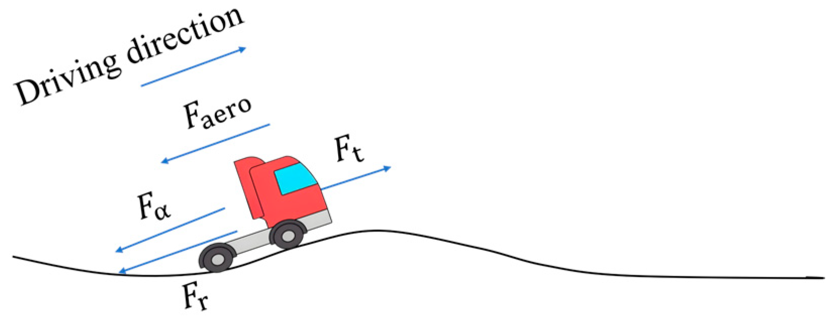
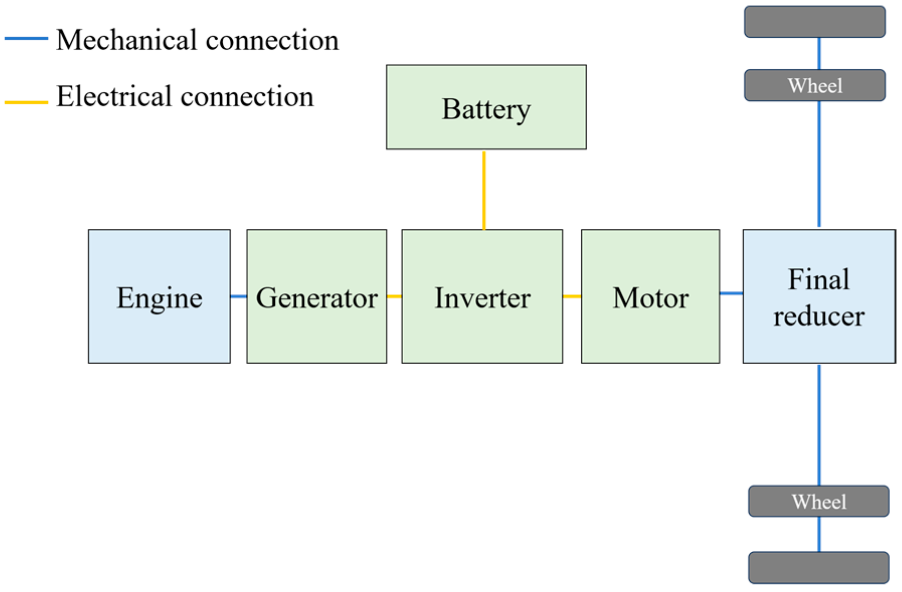
2.1. Heavy-Duty Series Hybrid Electric Vehicle Modelling

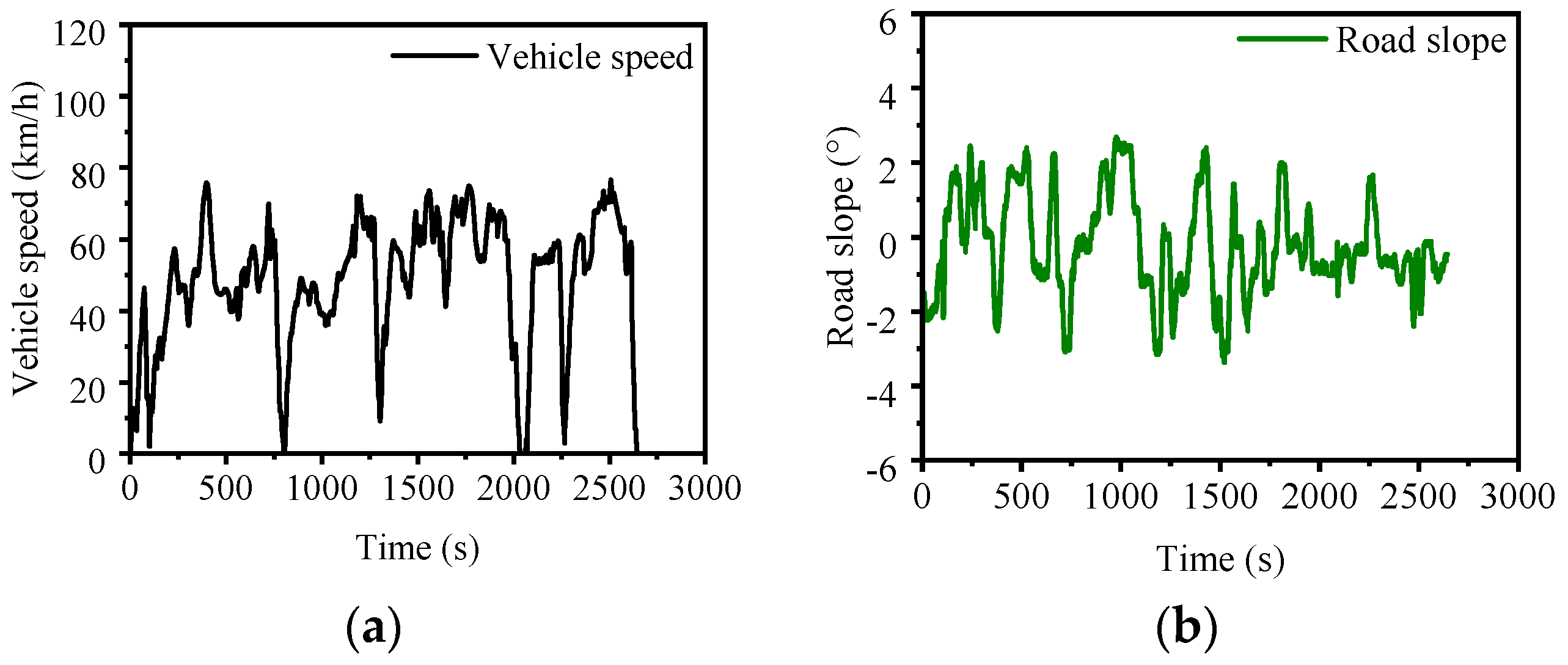
The vehicle model mainly includes an engine model, motor model, battery model, transmission system model, vehicle longitudinal dynamics model, and driver model.

The engine, generator, and drive motor are modeled using a steady-state MAP. The Brake specific fuel consumption (BSFC) MAP of the engine is shown in Figure 2.

The engine fuel consumption can be expressed as follows:

$${\dot{m}}_f=f\left(n_{eng},T_{eng}\right)$$

(1)

where $\dot{m}$_f represents the fuel consumption rate under the working condition; n_eng represents for current engine speed; T_eng represents the current engine torque.

The generator and motor are modeled in a similar way, with efficiency tabulated by the speed and torque of the generator and motor.

The modeling of the power battery adopts the method of an equivalent circuit, which regards the battery as an ideal voltage source and a resistor in series. The battery SOC can be calculated by ampere-hour integration, and the calculation formula is shown as follows.

$$SOC\left(t\right)={\displaystyle \frac{C·SOC\left(t_0\right)-{{\displaystyle \int }}_{t_0}^{t}Idt}{C}}$$

(2)

where C is the battery capacity; I is the battery charging and discharging current; SOC(t) indicates the current time battery.

The longitudinal force of the vehicle is shown in Figure 3. The vehicle needs to overcome the air resistance, rolling resistance, and slope resistance when driving, among which the air resistance and rolling resistance can be unified into the speed-related driving resistance formula according to the vehicle neutral coasting test data, as shown in Equation (3).

Figure 3. Longitudinal force diagram of vehicle.

Figure 3. Longitudinal force diagram of vehicle.

$$F_{aero}+F_r=A+Bv+C{v}^2$$

(3)

where F_aero is the air resistance; F_r is rolling resistance; v is the speed of the current vehicle; A, B, and C are driving resistance coefficients, respectively. The formula for calculating slope resistance is as follows:

$$F_{\alpha }=mgsin\theta$$

(4)

where m is vehicle mass; g is the gravitational acceleration; θ is the current road slope. At this time, the acceleration obtained by the vehicle is as follows:

$$a={\displaystyle \frac{F_t-A-Bv-C{v}^2-mgsin\theta }{m}}$$

(5)

where F_t represents the driving force of the vehicle, and a is the vehicle acceleration. The driving power of the whole vehicle can be expressed by Equation (6):

$$P_t=\left(ma+F_r+F_{areo}+mg\sin \theta \right)v$$

(6)

where P_t is the drive power.

The driver model uses a speed tracker based on PI control. The input is the deviation between the target speed and the actual speed, and after the proportional integral processing, the driving power demand of the current vehicle is calculated.

$$P_{dev}=K_P\left(v_{ref}-v\right)+K_i\int \left(v_{ref}-v\right)dt$$

(7)

where P_dev is the vehicle drive power demand, K_p and K_i are proportional coefficients and integral coefficients, respectively, v_ref is the reference speed, and v is the actual current speed of the model.

2.2. Test Route

The road conditions required for the study were collected from road experiments conducted in Shandong Province. The road type is a suburban section of a provincial road. The test vehicle is a heavy-duty fuel-powered vehicle with the same resistance parameters as the series hybrid prototype. Equipped with a slope sensor and CAN bus to obtain vehicle status information, such as vehicle speed, engine torque, and road slope information, the data sampling frequency is 10 Hz. The total collection range is more than 100 km. The 36 km continuous road section is extracted as the simulation test route, and the remaining road sections are used as the calibration and training dataset required for vehicle weight estimation, speed, and slope prediction. The 36 km simulation test route is not included in the training dataset, and its speed and slope data are shown in Figure 4.

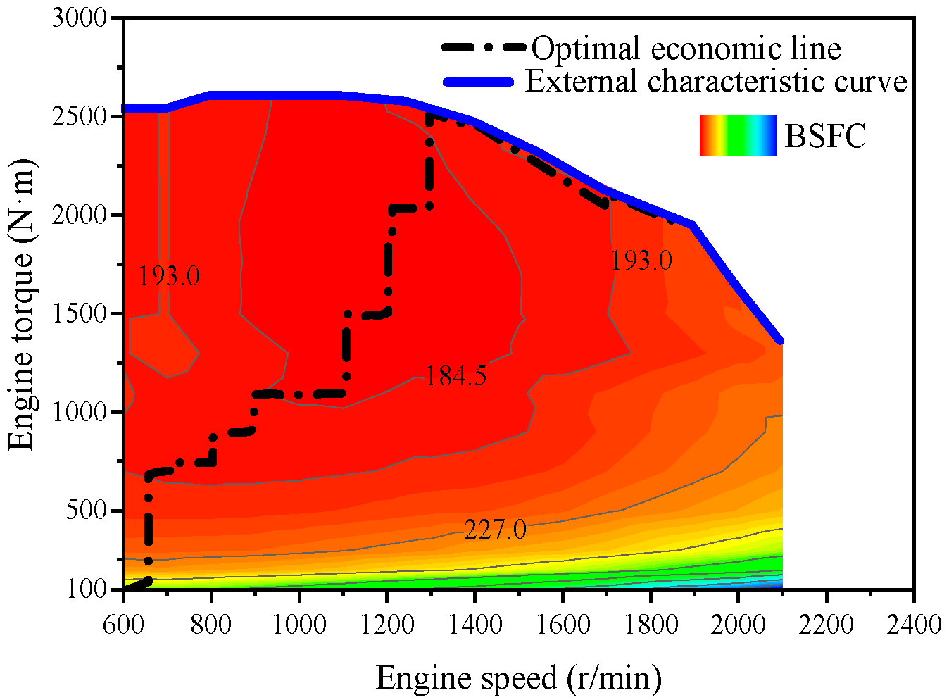
2.3. Vehicle Simulation Model Drive Power Validation

The vehicle drive power is the key input of energy management strategy optimization. Based on the driving power of the experimental vehicle on the test route, the driving power of the vehicle model is verified. The vehicle model is controlled by a rule-based thermostat strategy. The vehicle speed and vehicle drive power output by the model are compared with the experiment as shown in Figure 5.

The simulation model can accurately track the reference vehicle speed. To evaluate the consistency between the model and the experiment, the determination coefficient (R²) is used to characterize the interpretability of the experiment and the simulation, and the calculation process is shown in Equation (8). The R² value of the determination coefficient between the actual speed and the simulated speed is 0.986. The R² value between the simulated drive power and the experimental drive power is 0.943. It is concluded that the accuracy of the established model meets the requirements for subsequent research.

$$R^2=1-{\displaystyle \frac{{\displaystyle \sum _{\mathrm{i}=1}^N{(y_i-{\widehat{x}}_i)}^2}}{{\displaystyle \sum _{i=1}^N{(y_i-\overline{x})}^2}}}$$

(8)

where y_i is the predicted value, that is, the calculated value of the model; $\widehat{x}$_i is the true value, that is, the experimental collection value; $\overline{x}$ is the average value of the true value, that is, the average value of the experimental collection; N is the total number of calculated sequences.

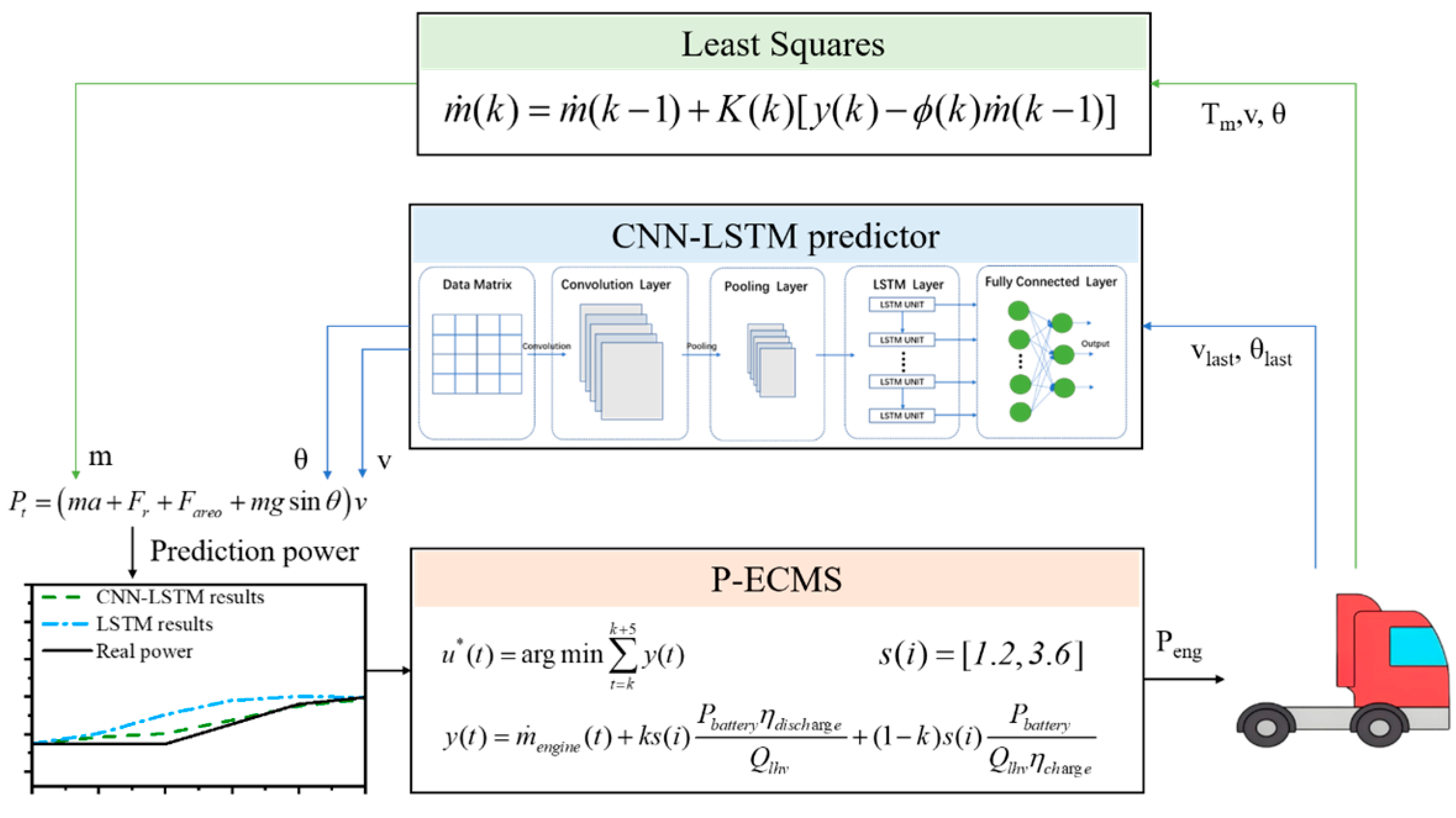
3. Predictive Energy Management Methodology

In order to cope with the complexities of the driving environment and large changes in the power demand of heavy-duty vehicles, a dynamic optimization energy management strategy was developed by using a drive power prediction model. The drive power prediction model obtains the mass, speed, and slope of the future time domain required for the drive power calculation through the identification algorithm and prediction model. Based on the drive power, the mode-switching timing and power distribution of the hybrid powertrain are optimized based on the framework of the regular energy management strategy and combined with the forecast information to improve the fuel economy. Figure 6 illustrates the framework for predictive energy management.

3.1. Mass Estimation

The identification of vehicle mass is based on the least squares method with a forgetting factor [18]. According to the longitudinal dynamics model of Equation (6), slope and speed are measured, acceleration is the velocity first-order differential filter, and driving force can be calculated by the driving motor. Given the principle of least squares, let y(k) = Ft − (A + Bv + Cv²), which represents the actual output value of the system at time k; let $\varphi \left(k\right)=a+gsin\left(\theta \right)$, which represents the observed value of the system at time k; the mass m is the parameter to be identified, and its optimal estimate at time k is assumed to be $\dot{m}$(k). The estimation model of vehicle weight is as follows:

$$\left\{\begin{array}{c}\dot{m}(k)=\dot{m}(k-1)+K(k)[y(k)-\varphi (k)\dot{m}(k-1)]\\ K(k)={\displaystyle \frac{P_{RLS}(k-1){\varphi }^T(k)}{{\lambda }_{RLS}+\varphi (k)P{(k-1)}_{RLS}{\varphi }^T(k)}}\\ P{(k)}_{RLS}={\displaystyle \frac{1}{{\lambda }_{RLS}}}(1-K(k)\varphi (k))P{(k-1)}_{RLS}\end{array}\right.$$

(9)

where K(k) represents the system gain matrix, and P(k)_RLS is the covariance matrix of state variables in RLS. The empirical formula selected by λ_rls is as follows:

$${\lambda }_{RLS}=1-{\displaystyle \frac{1}{{0.975}^{\mathrm{t}}}}$$

(10)

where t is the execution time of the algorithm from the beginning to the present.

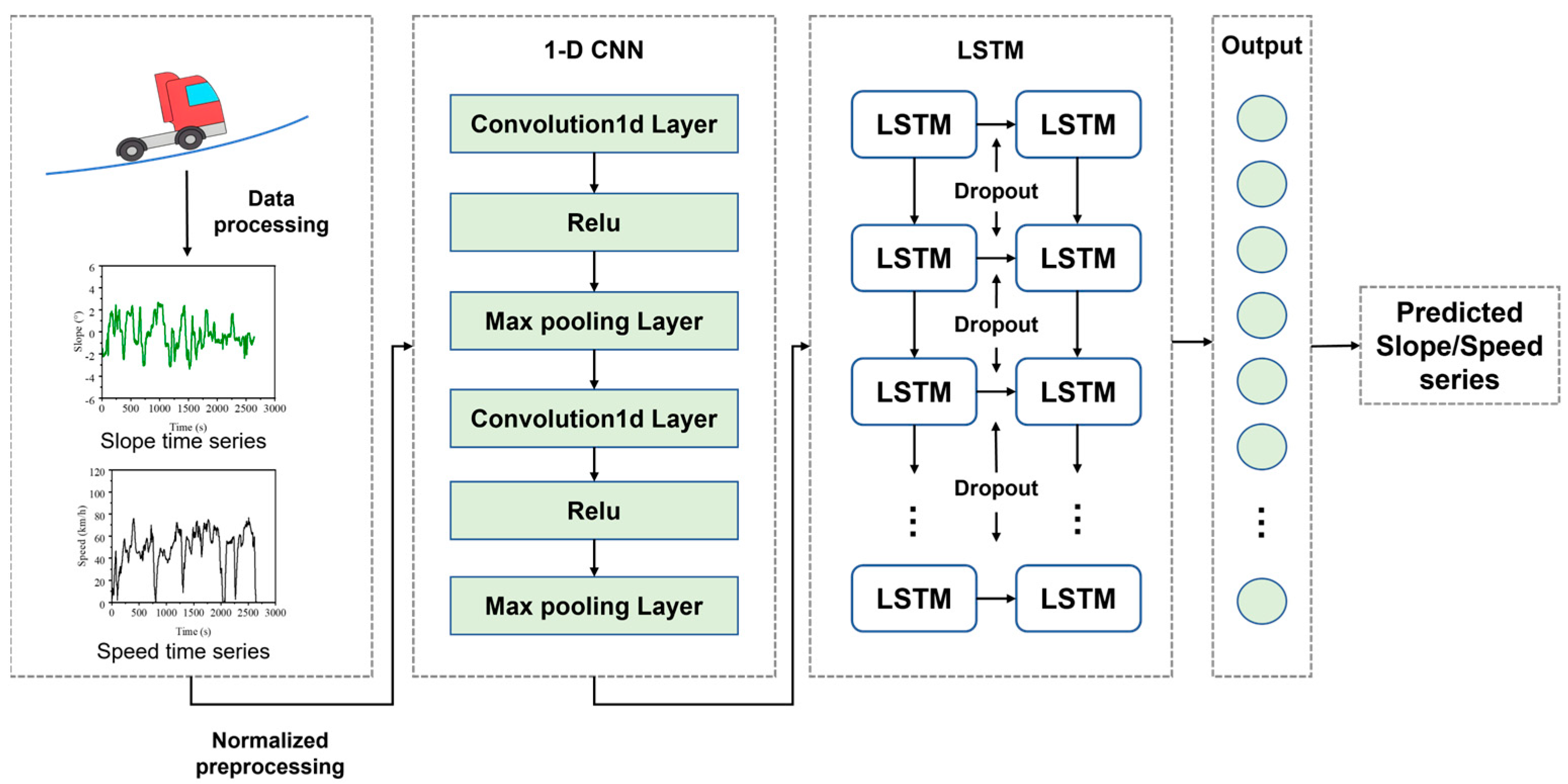
3.2. Speed and Slope Prediction

Based on previous work [19], a prediction framework for speed and slope estimation was developed using a combination of a convolutional neural network (CNN) and a long short-term memory (LSTM) neural network. A one-dimensional CNN is employed to extract spatial dimension features of the speed and slope timing series, and LSTM is used to mine temporal dimension features of the speed and slope timing series. Speed and slope predictions were made separately, but the same model structure was used.

A CNN and LSTM can form a hybrid network structure to extract spatiotemporal features in time series. The CNN first convolves the original sequence and extracts the spatial features through activation, pooling, and other operations. The number of filters is 64, and the dimension is 1 × 10. The window size of the pooling layer is 5. The extracted spatial features are input into LSTM, and after processing by neurons in each layer of the structure, the time features are extracted. The subpackage contains two layers of LSTM, each with an output dimension of 100, and each layer uses the Dropout operation to randomly set some of the hidden layer’s weights or outputs to 0. The output of the LSTM model is transmitted to the fully connected layer, and the output of the fully connected layer is the result of the time series prediction, and the number of neurons in the fully connected layer is the same as the expected prediction time step. The overall architecture of the model is shown in Figure 7:

The data required for model training and validation are collected from vehicle experiments, as shown in Section 2.2. The method of a sliding window is used to extract raw data to establish training and verification samples. To predict the future, we collect 5 s data from the 10 s data from vehicle driving and extract usable samples with 15 s as the window length. A total of 80% of the samples in the dataset were used for model training, and 20% were used for testing.

3.3. Future Drive Power Calculation

According to Equation (5) of the vehicle longitudinal dynamics model, the calculation of driving power requires not only the vehicle weight and road slope but also acceleration. The future acceleration is obtained by differentiating the predicted velocity. However, performing a first-order differentiation on small time steps amplifies minor fluctuations in the original signal, introducing noise into the acceleration calculation. A Fourier transform analysis reveals that most of the noise in the acceleration signal is concentrated above 0.5 Hz. To mitigate this, a first-order low-pass filter is applied, with a cutoff frequency set at 0.5 Hz. The corresponding transfer function is shown in Equation (11).

$$a={\displaystyle \frac{s}{\tau s+1}}v$$

(11)

where τ represents the time constant (the specific value is related to the cutoff frequency, such as in Equation (12)), a is the acceleration, and v is the vehicle speed.

$$\tau ={\displaystyle \frac{1}{2\pi f_c}}$$

(12)

where f_c represents the end frequency.

Based on the estimation of vehicle weight and the prediction of future acceleration and slope, the future drive power series can be calculated through the longitudinal dynamics model with Equation (6).

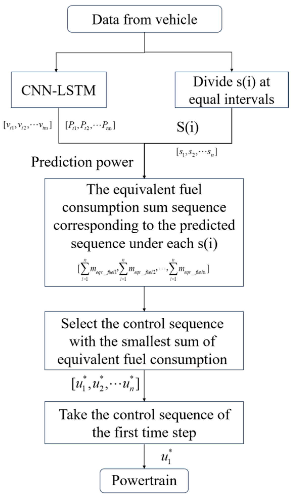
3.4. Predictive ECMS

To optimize the energy distribution between engines and motors, a predictive ECMS (recorded as P-ECMS) strategy based on charge depleting/charge sustaining (CD/CS) has been developed. According to the prediction information, the switching selection of CD/CS is optimized, and the engine power is optimized according to the principle of minimum equivalent fuel consumption in the CS stage. The CD/CS switching rules adopted are shown in

Table 2. Rule-based EMS.

Mode	Switch Conditions	Engine Power Demand	Motor Power Demand
CS	SOC ≤ e1 || (SOC > e1 and Preq > p1)	Pa	Preq
CD	SOC > e1 and Preq ≤ p1	0	Preq
Mechanical braking	Pdemand < 0 and (v ≤ 10 km/h || SOC ≥ e2)	0/Pidle	0
Motor braking energy recovery	Pdemand < 0 and v > 10 km/h and SOC < e2	0/Pidle	Preq

. When the SOC is lower than the set threshold e1 or the required power is greater than the set threshold p1, the engine starts and enters the series drive. At this time, the engine operates at a fixed working condition point, with three optional points: high, middle, and low. The selection is based on the actual SOC, and the specific SOC switching threshold is obtained through experimental calibration. When the SOC is higher than e1 and the required power is less than p1, it enters the power consumption mode, and the engine does not run. In the rules, e1 is 0.3, e2 is 0.9, and p₁ adopts the upper limit of low-speed section driving power in the China Heavy-Duty Commercial Vehicle Test Cycle for Tractor-Trailers (CHTC-TT), which is 110 kW. P_idle is the idle power.

When the power changes greatly, the rule-based strategy will cause the engine to start and stop frequently, and after starting, the energy can only be distributed according to the fixed operating point or the power to follow, until the SOC or the demand power changes and enters other modes.

When predictive information is available, the engine starting time and power distribution can be optimized according to the working condition characteristics to reduce energy consumption. The starting time is optimized by means of a power average. When the predicted power average in the next 5 s is higher than the starting threshold, the drive mode is switched from CD to CS. Once in the CS mode, the ECMS is adopted to convert the instantaneous power consumption into the instantaneous fuel consumption through the equivalent fuel factor and then summed with the instantaneous fuel consumption of the engine to obtain the instantaneous equivalent fuel consumption. Finally, the control quantity corresponding to the minimized instantaneous equivalent fuel consumption is solved. To achieve fuel economy optimization during vehicle operation and capture the real-time condition change, the equivalent factor and energy consumption are optimized under the prediction boundary. The calculation process is shown in Figure 8.

The instantaneous equivalent energy consumption can be expressed as follows:

$${\dot{m}}_{equ\_fuel}={\dot{m}}_{engine}+{\dot{m}}_{battery}$$

(13)

where $\dot{m}$_{equ_fuel} represents instantaneous equivalent fuel consumption, $\dot{m}$_engine indicates instantaneous fuel consumption, the instantaneous power consumption of the power battery is equivalent to the instantaneous fuel consumption, and $\dot{m}$_battery can be represented by Equation (14).

$${\dot{m}}_{battery}=ks(i){\displaystyle \frac{P_{battery}{\eta }_{discha}}{Q_{lhv}}}+(1-k)s(i){\displaystyle \frac{P_{battery}}{Q_{lhv}{\eta }_{cha}}}$$

(14)

where Q_lhv is the low calorific value of diesel oil, s(i) is the equivalent fuel factor, k indicates the working state of the battery. Zero is used for charging, and one is used for discharging. η_discha represents battery discharge efficiency, and η_cha stands for battery charging efficiency.

The desired control sequence and optimization constraint range can be expressed as follows:

$$u^{*}(t)=\arg \min {\displaystyle \sum _{t=k}^{k+5}y(t)}$$

(15)

$$\left\{\begin{array}{c}{n}_{\min }\le n\le n_{\max }\\ T_{\min }\le T\le T_{\max }\\ P_{\min }\le P\le P_{\max }\\ SO{C}_{\min }\le SOC\le SO{C}_{\min }\end{array}\right.$$

(16)

where y(t) is the equivalent energy consumption at each moment, as shown in Equation (17), and t is the current calculation time; u is the control sequence corresponding to the minimum value of the total equivalent energy consumption of the future 5 s, that is, the engine power sequence of the future 5 s. Only the first value of this sequence will be an output of the vehicle model as a command, and the same rolling calculation will continue in the next step. Constraints on the system include speed, torque, and power limits for the engine, generator, and drive motor, as well as SOC and charge-discharge power limits for the battery.

$$y(t)={\dot{m}}_{engine}(t)+ks(i){\displaystyle \frac{P_{battery}{\eta }_{disch\arg e}}{Q_{lhv}}}+(1-k)s(i){\displaystyle \frac{P_{battery}}{Q_{lhv}{\eta }_{ch\arg e}}}$$

(17)

When calculating the total energy consumption within the 5 s prediction boundary, s(i) calculates the total energy consumption separately over a range of equivalent factors from 1.2 to 3.6, using a step size of 0.1. The range of equivalent factors is divided according to the CHTC-TT simulation results, with increasing engine involvement from 1.2 to 3.6. The step size of 0.1 strikes a balance between computational efficiency and accuracy. The CHTC-TT simulation with different equivalent factors is shown in Figure 9. As the equivalent fuel factor increases, the SOC at the end is higher, indicating a greater reliance on the engine to meet power demand. By optimizing the equivalent factor, overall vehicle energy consumption can be minimized.

In the evaluation of energy consumption, in order to eliminate the impact of electricity on fuel consumption, the comprehensive energy consumption is calculated through the electric energy consumption conversion method specified in GB/T 37340-2019 (China National Standards: Conversion Methods for Energy Consumption of Electric Vehicles) [20]:

$$F{C}_{equ}=E\times F_E+F{C}_{eng}$$

(18)

FC_equ stands for the equivalent 100 km fuel consumption, in L/100 km; E is the electric consumption, and the unit is kW·h/100 km; F_E is the fuel energy factor, which is calculated based on the calorific value of fuel and electricity according to China National Standards; it is used to convert electricity consumption into fuel consumption, and the unit is L/kW·h; the fuel energy factor of 0# diesel can be 0.1042; FC_eng is the vehicle fuel consumption per 100 km, and the unit is L/100 km.

4. Results and Discussion

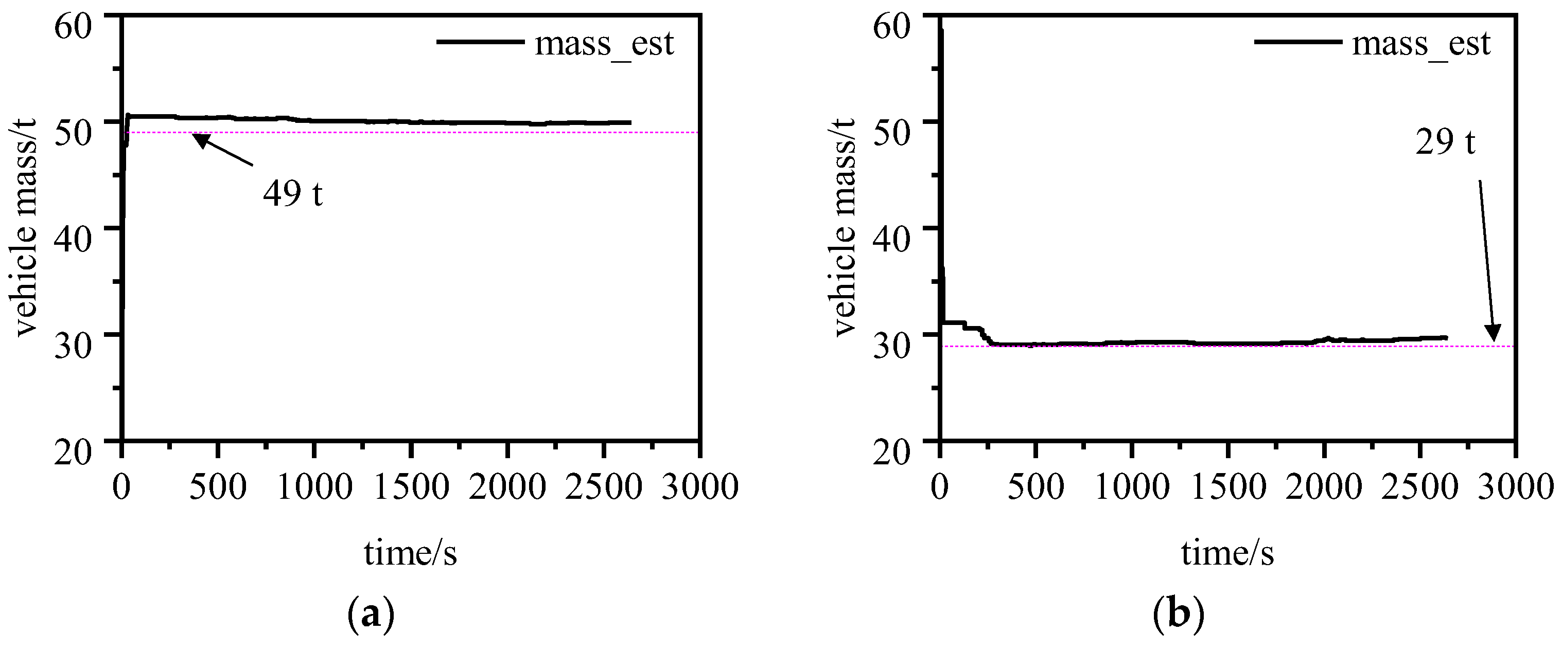
4.1. Mass Estimation Results

In order to verify the results of vehicle weight estimation, the collected road spectrum information is imported into the established simulation platform. Driven by the driver model, the simulation platform can output the driving torque, speed, and slope information required for vehicle weight estimation. The slope is set to be available from maps and positioning information, so it is assumed to be known from the vehicle weight estimation. The estimated effect is verified at 49 t full load and 29 t nearly half load, and the results are shown in Figure 10. Under the test condition of a 49 t vehicle weight, the vehicle weight estimation algorithm estimates the final vehicle weight to be 49.9 t, and the error is 1.9%. In the 29 t test, the estimated result is 29.6 t, with an error of 2.1%. The time between the first stabilization of the algorithm’s vehicle weight estimate and the final convergence of 95% to 105% of the vehicle weight is defined as the convergence time of the vehicle weight estimate, and the convergence times of 49 t and 29 t are 13.2 s and 16.7 s, respectively. The accuracy and convergence time of vehicle weight estimation can meet the developments of predictive energy management.

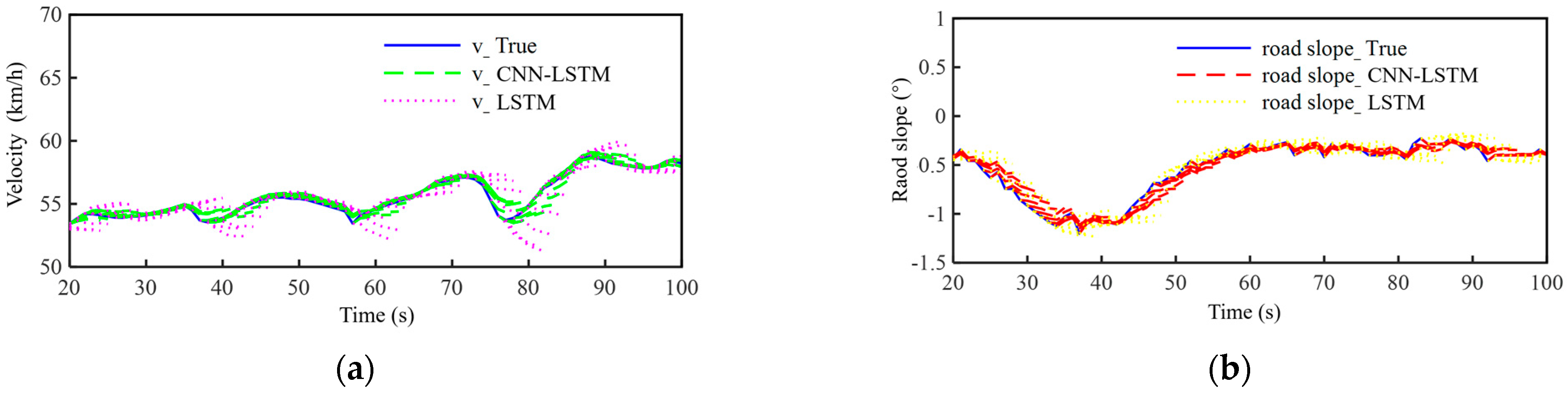
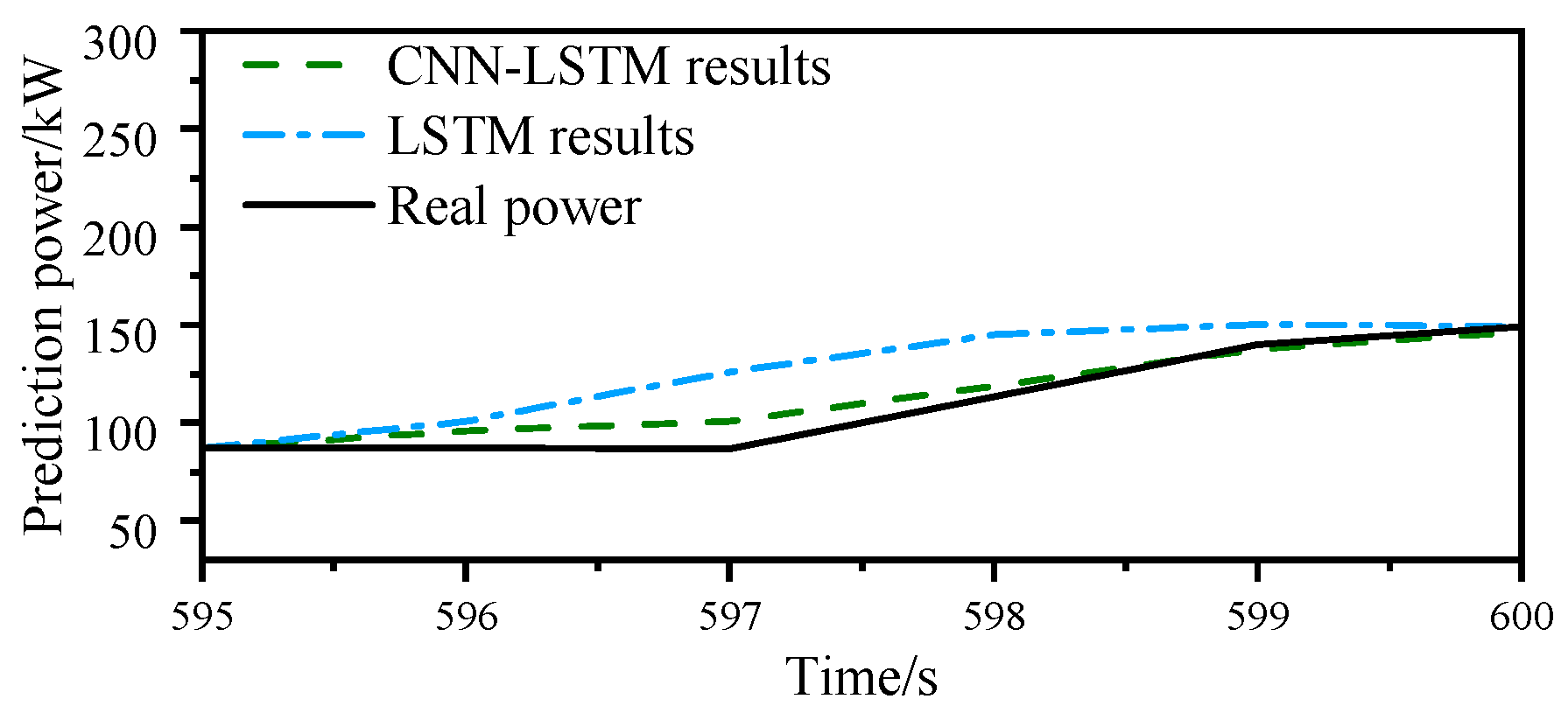
4.2. Drive Power Prediction

CNN-LSTM and LSTM were used as predictors, respectively, and the model was trained based on the training dataset. The LSTM was used as the baseline model for comparison to evaluate the effect of adding convolution. After the training, the model was tested on the collected test path spectrum. The prediction time of the two models is set to 5 s, and the prediction effect of 20–100 s in the test road spectrum is shown in Figure 11, where the speed collected by the sensor and the road slope are recorded as the reference speed v_True and road slope_True.

The average value of RMSE was used to evaluate the prediction accuracy. That is, the RMSE of the 5 s predicted value and the true value of each step is calculated, and the RMSE of all steps is summed and averaged to characterize the prediction accuracy.

$$RMSE=\sqrt{{\displaystyle \sum }_{i=1}^n{\left(y_i-x_i\right)}^2/n}$$

(19)

where x_i represents the actual value, and y_i represents the predicted value.

Table 3. Prediction performance of LSTM and CNN-LSTM models.

Model	RMSE of Speed Prediction (km/h)	RMSE of Slope Prediction (°)	RMSE of Power Prediction (kW)
LSTM	1.5	0.162	17.2
CNN-LSTM	1.4 (−6.7%)	0.141 (−13.0%)	14.8 (−14.0%)

shows the performance of different prediction models. When the CNN-LSTM predictor is used to predict the speed, the average one-step RMSE between the predicted value and the true value is 1.4 km/h. When predicting the slope, the RMSE of the predicted value and the true value is 0.141°. The RMSE is 1.5 km/h when only the LSTM model is used to predict the speed and 0.162° when predicting the slope. The prediction error of the proposed CNN-LSTM prediction model is smaller than that of the LSTM prediction model, indicating that the prediction accuracy of CNN-LSTM is greater than that of the LSTM model under the current data and prediction step size. It is difficult for LSTM to detect the change trend after 5 s relying only on the time series features, so the output value is closer to the change trend before 5 s, resulting in the overall trend lag of the output results, and thus the prediction accuracy decreases. In contrast, the CNN-LSTM network that integrates the temporal and spatial features achieves better results, indicating that the integration of spatial features is helpful for improving the ability of short-time multi-step prediction of slope series.

The speed and slope predicted by CNN-LSTM and LSTM are, respectively, calculated by Equation (6), and the predicted results of 595~600 s are shown in Figure 12. Because CNN-LSTM uses more data features, it can grasp the trend of data change better, and the predicted power is closer to the real power. In the test path spectrum, the average RMSE of the single predicted power curve and the reference actual power curve is 14.8 kW, and the RMSE of the future required power calculated using the predicted information of the CNN-LSTM is 17.2 kW. When the CNN-LSTM is trained and predicted directly using the required power, the average RMSE per time between the predicted value and the reference value is 17.3 kW. The CNN-LSTM hybrid prediction model is more accurate than the single LSTM model.

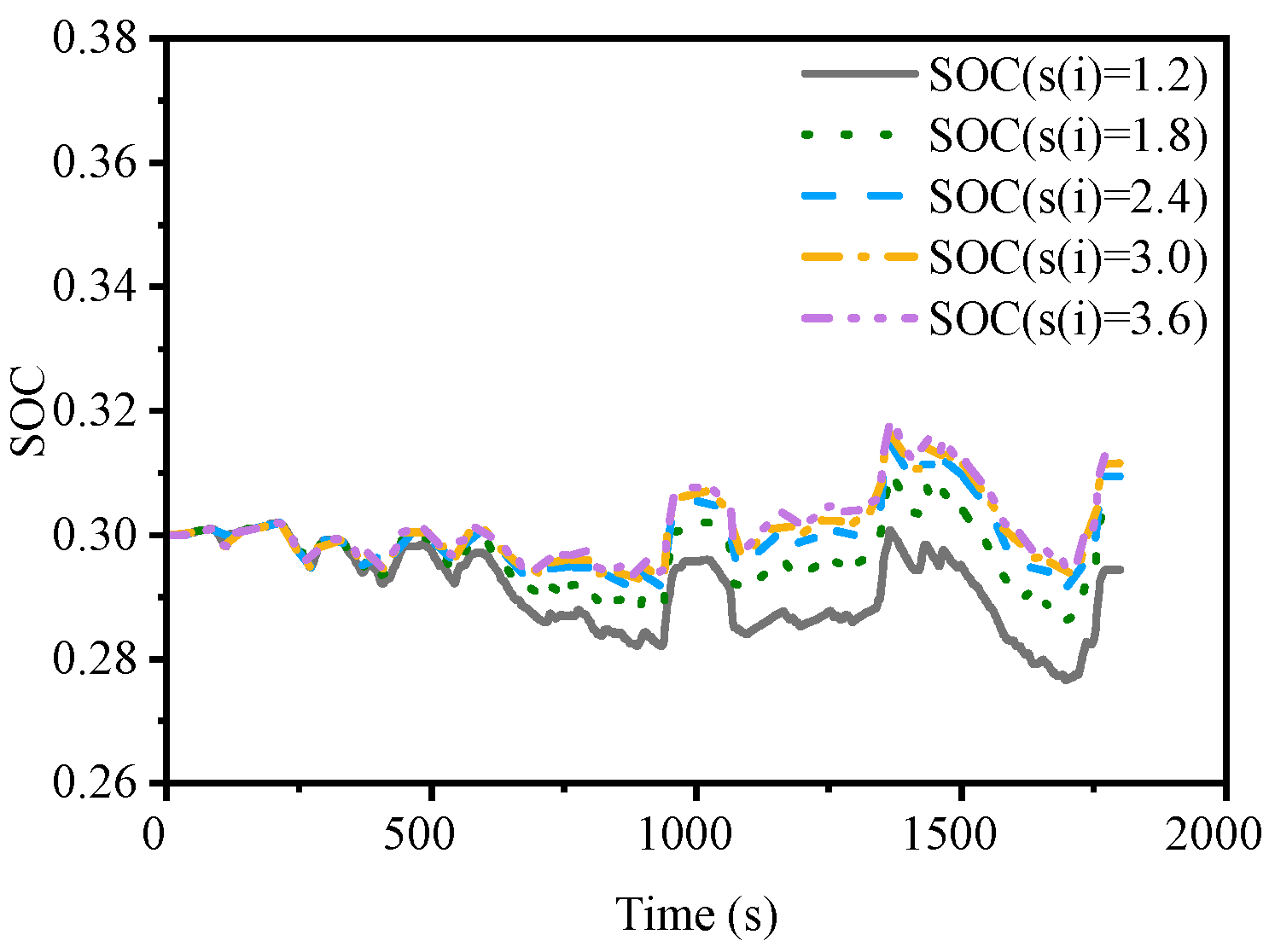
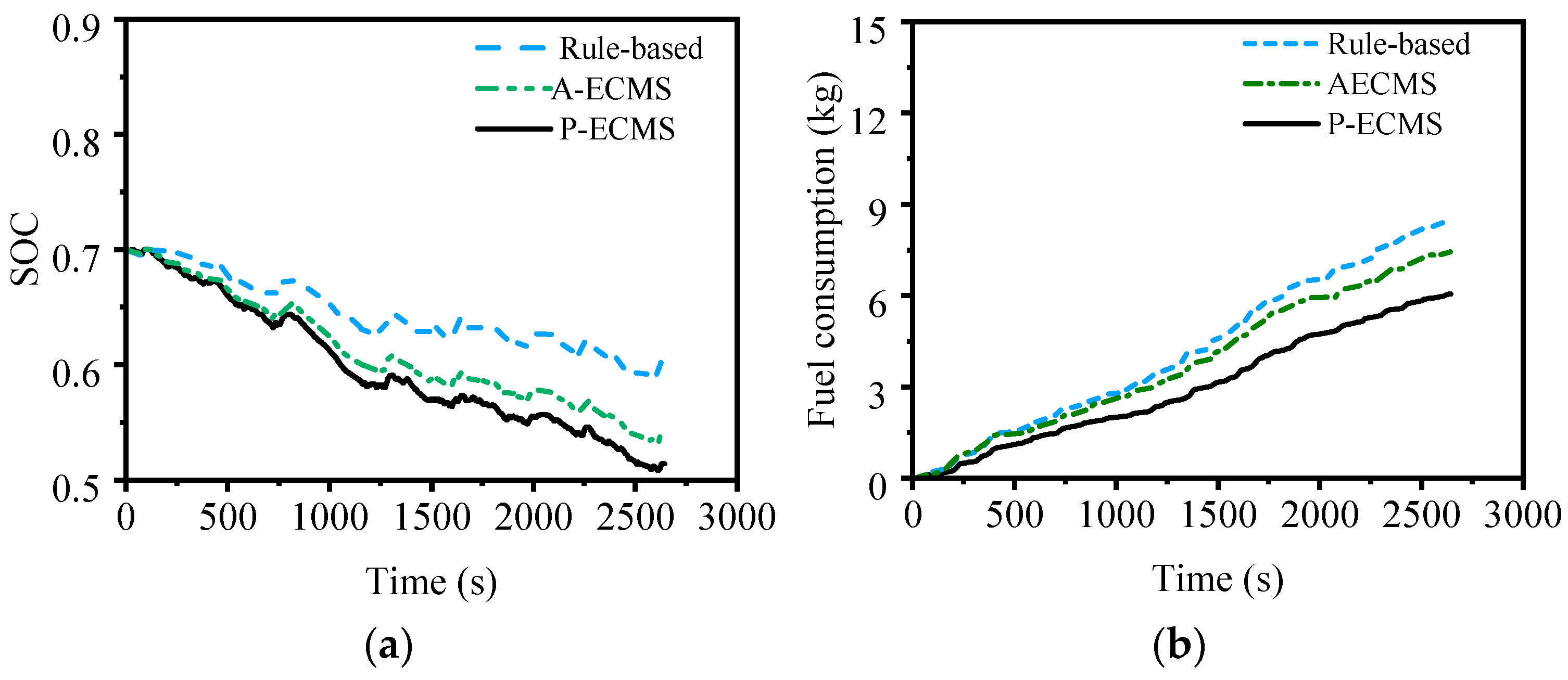
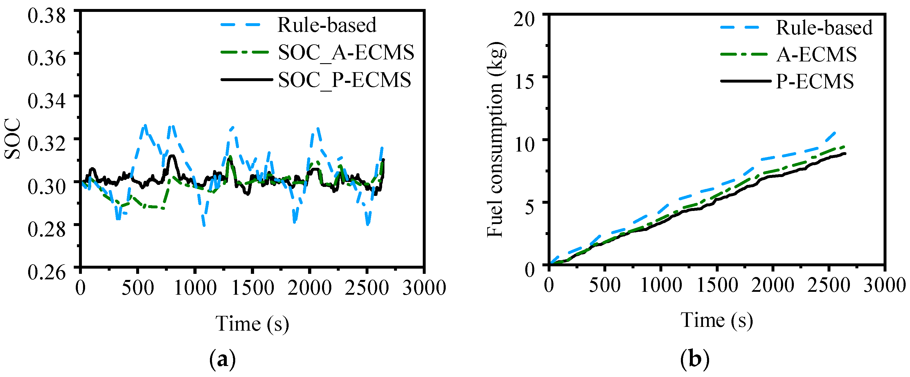
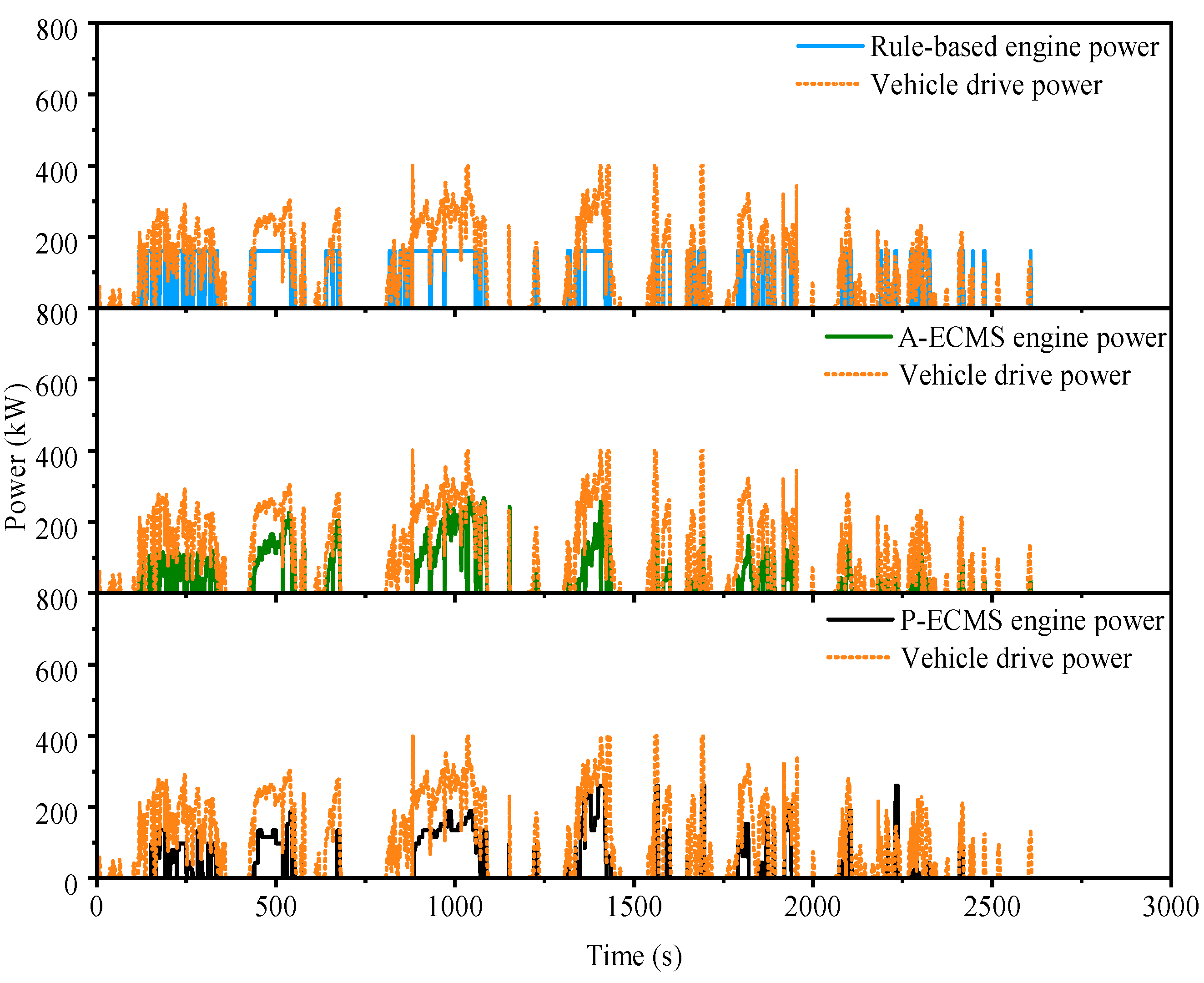
4.3. Energy Consumption of EMSs

The above rule strategy and the SOC feedback-based adaptive ECMS [21] (recorded as A-ECMS) are used as comparison strategies to verify the energy consumption optimization effect introduced by the forecast information.

The simulation results of the P-ECMS, A-ECMS, and rule-based control strategy are shown in Figure 13 and Figure 14. Figure 13 shows the SOC and fuel consumption results in the CD mode. Compared with the A-ECMS and rule-based strategy, the P-ECMS has faster power reduction and lower fuel consumption. Figure 14 shows the simulation results in the CS mode. The P-ECMS showed good energy-saving performance.

Table 4. Energy consumption under the CD and CS modes.

Operation Mode	EMS	Fuel Consumption (L/100 km)	Final SOC	Equivalent Energy Consumption (L/100 km)
CD	Rule	24.32	0.603	27.10
	A-ECMS	21.14	0.531	26.00
	P-ECMS	20.08	0.514	25.43
CS	Rule	34.88	0.321	34.28
	A-ECMS	29.99	0.309	29.73
	P-ECMS	29.42	0.310	29.13

shows the energy consumption results in the CD and CS modes as shown in Figure 13 and Figure 14. In the CD mode, the average equivalent fuel consumption per 100 km for the P-ECMS is 25.84 L/100 km, and the average equivalent fuel consumption per 100 km of the P-ECMS is relatively reduced by 1.4% and 7.5% compared with the energy management strategy based on the A-ECMS and rule-based strategy. In the CS mode, the final SOC of each strategy can remain near the threshold, but the final SOC of the P-ECMS is slightly lower than that of the A-ECMS and rule-based strategy. In terms of fuel consumption per 100 km, the P-ECMS is lower than the A-ECMS and rule-based strategy, which indicates that the P-ECMS is more inclined to use electric power for driving while ensuring power maintenance. The average equivalent fuel consumption per 100 km of the P-ECMS is 29.84 L/100 km, which is 1.2% lower than that of the A-ECMS and 11.8% lower than that of the rule-based strategy.

Figure 15 shows a time sequence of engine power with different strategies. The A-ECMS and P-ECMS rely on the equivalent fuel factor regulation, and the engine start working time is less than the rule-based strategy. The rule-based strategy maintains a relatively high-power output after starting, so fuel consumption is significantly higher than other strategies, and the SOC trajectory declines most slowly. Compared with the A-ECMS, the P-ECMS avoids the mode switching caused by the rapid change in demand power, and the engine working condition is more stable. As shown in Figure 5, Figure 6, Figure 7, Figure 8, Figure 9, Figure 10, Figure 11, Figure 12, Figure 13, Figure 14 and Figure 15, the P-ECMS engine output power is stable during the period from 900 s to 1000 s, while the A-ECMS and rule-based strategies have the phenomenon of rapid engine start and stop when the vehicle demand power is less than 110 kW (the switching threshold of the CD stage in high and low working conditions).

5. Conclusions

The predictive ECMS is realized through the identification of vehicle weight and the prediction of future speed and slope. The P-ECMS can automatically select the best equivalent factor based on the prediction information.

The mass estimation method based on least squares can control the estimation error within 3% in the actual road data collected. When the actual vehicle weight is 49 t, the estimated result is 49.9 t, with an error of 1.9%. When the actual vehicle weight is 29 t, the estimated result is 29.6 t, with an error of 2.1%.

The CNN-LSTM hybrid prediction model is used to predict the future vehicle speed and road slope. The hybrid model can obtain the spatial features of the data structure, which is richer than the simple time series data features. In the prediction time domain of 5 s, the average RMSE of the drive power predicted by the CNN-LSTM model and the real drive power is 14.8 kW, and the average RMSE of the drive power calculated by LSTM only is 17.2 kW. This indicator is 17.3 kW when the CNN-LSTM model is used to predict the drive power directly. The CNN-LSTM hybrid model has a 14.0% higher prediction accuracy than LSTM.

The developed P-ECMS achieves energy consumption improvements in both the CD and CS modes. When the vehicle is fully loaded and in the CD mode, the energy consumption is 25.43 L/100 km, which is 2.2% and 6.2% less than the A-ECMS and the original rule-based strategy. In the CS mode, the energy consumption is 29.13 L/100 km, which is 2.0% lower than the A-ECMS and 15.0% less than the original rule-based strategy.

References

1. Xia, X.; Bhatt, N.P.; Khajepour, A.; Hashemi, E. Integrated Inertial-LiDAR-Based Map Matching Localization for Varying Environments. IEEE Trans. Intell. Veh. 2023, 8, 4307–4318. [Google Scholar] [CrossRef]
2. Lü, X.; Li, S.; He, X.H.; Xie, C.; He, S.; Xu, Y.; Fang, J.; Zhang, M.; Yang, X. Hybrid Electric Vehicles: A Review of Energy Management Strategies Based on Model Predictive Control. J. Energy Storage 2022, 56, 106112. [Google Scholar] [CrossRef]
3. İşbitirici, A.; Giarré, L.; Xu, W.; Falcone, P. LSTM-Based Virtual Load Sensor for Heavy-Duty Vehicles. Sensors 2024, 24, 226. [Google Scholar] [CrossRef] [PubMed]
4. Wang, B.; Wang, H.; Wu, L.; Cai, L.; Pi, D.; Wang, E. Truck Mass Estimation Method Based on the On-Board Sensor. Proc. Inst. Mech. Eng. Part D J. Automob. Eng. 2020, 234, 2429–2443. [Google Scholar] [CrossRef]
5. Mahyuddin, M.N.; Na, J.; Herrmann, G.; Ren, X.; Barber, P. Adaptive Observer-Based Parameter Estimation with Application to Road Gradient and Vehicle Mass Estimation. IEEE Trans. Ind. Electron. 2014, 61, 2851–2863. [Google Scholar] [CrossRef]
6. Cai, L.; Wang, H.; Jia, T.; Peng, P.; Pi, D.; Wang, E. Two-Layer Structure Algorithm for Estimation of Commercial Vehicle Mass. Proc. Inst. Mech. Eng. Part D J. Automob. Eng. 2020, 234, 378–389. [Google Scholar] [CrossRef]
7. Li, X.; Ma, J.; Zhao, X.; Wang, L. Intelligent Two-Step Estimation Approach for Vehicle Mass and Road Grade. IEEE Access 2020, 8, 218853–218862. [Google Scholar] [CrossRef]
8. Pérez, W.; Tulpule, P.; Midlam-Mohler, S.; Rizzoni, G. Data-Driven Adaptive Equivalent Consumption Minimization Strategy for Hybrid Electric and Connected Vehicles. Appl. Sci. 2022, 12, 2705. [Google Scholar] [CrossRef]
9. Li, Q.; Cheng, R.; Ge, H. Short-Term Vehicle Speed Prediction Based on BiLSTM-GRU Model Considering Driver Heterogeneity. Phys. A Stat. Mech. Its Appl. 2023, 610, 128410. [Google Scholar] [CrossRef]
10. Zhang, J.; Peng, T.; Mo, L.; Hu, X.; Wang, X. Research on Highway Slope Monitoring Data Prediction Based on Long Short-Term Memory Network. IOP Conf. Ser. Earth Environ. Sci. 2020, 571, 012087. [Google Scholar] [CrossRef]
11. Chen, L.; Liao, Z.; Ma, X. Nonlinear Model Predictive Control for Heavy-Duty Hybrid Electric Vehicles Using Random Power Prediction Method. IEEE Access 2020, 8, 202819–202835. [Google Scholar] [CrossRef]
12. Beckers, C.; Besselink, I.; Nijmeijer, H. Combined Rolling Resistance and Road Grade Estimation Based on EV Powertrain Data. IEEE Trans. Veh. Technol. 2023, 72, 3201–3213. [Google Scholar] [CrossRef]
13. Liu, J.; Qin, T.; Chen, D.; Wang, G.; Chen, T. Driving Power Prediction of Heavy Commercial Vehicles Based on Multi-Task Learning. IFAC-PapersOnLine 2024, 58, 397–402. [Google Scholar] [CrossRef]
14. Wang, J.; Liu, K.; Yamamoto, T. Improving Electricity Consumption Estimation for Electric Vehicles Based on Sparse GPS Observations. Energies 2017, 10, 129. [Google Scholar] [CrossRef]
15. Lu, L.; Zhao, H.; Liu, X.; Sun, C.; Zhang, X.; Yang, H. MPC-ECMS Energy Management of Extended-Range Vehicles Based on LSTM Multi-Signal Speed Prediction. Electronics 2023, 12, 2642. [Google Scholar] [CrossRef]
16. Tian, H.; Wang, X.; Lu, Z.; Huang, Y.; Tian, G. Adaptive Fuzzy Logic Energy Management Strategy Based on Reasonable SOC Reference Curve for Online Control of Plug-in Hybrid Electric City Bus. IEEE Trans. Intell. Transp. Syst. 2018, 19, 1607–1617. [Google Scholar] [CrossRef]
17. Kim, H.; Son, H.; Kim, H.; Hwang, S. Development of an Advanced Rule-Based Control Strategy for a PHEV Using Machine Learning. Energies 2018, 11, 89. [Google Scholar] [CrossRef]
18. Liu, Z.; Cheng, S.; Liu, J.; Wu, Q.; Li, L.; Liang, H. A Novel Braking Control Strategy for Hybrid Electric Buses Based on Vehicle Mass and Road Slope Estimation. Chin. J. Mech. Eng. (Engl. Ed.) 2022, 35, 150. [Google Scholar] [CrossRef]
19. Qin, T.; Yao, Z.; Fan, H.; Xia, R.; Chen, T. Vehicle Road Grade Prediction Based on CNN-LSTM. IFAC-PapersOnLine 2023, 56, 3066–3071. [Google Scholar] [CrossRef]
20. GB/T 37340-2019; Conversion Methods for Energy Consumption of Electric Vehicles. National Standard of the People’s Republic of China: Beijing, China, 2019.
21. Yao, D.; Lu, X.; Chao, X.; Zhang, Y.; Shen, J.; Zeng, F.; Zhang, Z.; Wu, F. Adaptive Equivalent Fuel Consumption Minimization Based Energy Management Strategy for Extended-Range Electric Vehicle. Sustainability 2023, 15, 4607. [Google Scholar] [CrossRef]
Figure 1. Heavy-duty series hybrid electric vehicle architecture.
Wevj 16 00186 g001
Figure 2. Engine BSFC MAP.
Wevj 16 00186 g002
Figure 4. (a)Vehicle speed with test condition. (b) Vehicle slope with test condition.
Wevj 16 00186 g004
Figure 5. Validation of simulation model. (a) Vehicle speed validation. (b) Drive power validation.
Wevj 16 00186 g005
Figure 6. Predictive energy management framework.
Wevj 16 00186 g006
Figure 7. The proposed CNN-LSTM hybrid model architecture.
Wevj 16 00186 g007
Figure 8. Predictive ECMS calculation flow chart.
Wevj 16 00186 g008
Figure 9. SOC trajectories with different equivalent factors.
Wevj 16 00186 g009
Figure 10. (a) The 49 T estimation result. (b) The 29 T estimation result.
Wevj 16 00186 g010
Figure 11. (a) Vehicle velocity prediction result. (b) Road slope prediction result.
Wevj 16 00186 g011
Figure 12. Predicted drive power in a single step of 595 s.
Wevj 16 00186 g012
Figure 13. Performance of different EMS in CD mode. (a) SOC trajectories. (b) Energy consumptions.
Wevj 16 00186 g013
Figure 14. Performance of different EMS in CS mode. (a) SOC trajectories. (b) Energy consumptions.
Wevj 16 00186 g014
Figure 15. Time sequence diagram of engine power with different EMSs.
Wevj 16 00186 g015