Article

Estimation of Vehicle Mass and Road Slope for Commercial Vehicles Utilizing an Interacting Multiple-Model Filter Method Under Complex Road Conditions

1
School of Vehicle and Traffic Engineering, Henan Institute of Technology, Xinxiang 453000, China
2
School of Mechanical and Power Engineering, Nanjing University of Technology, Nanjing 211816, China
World Electr. Veh. J. 2025, 16(3), 172; https://doi.org/10.3390/wevj16030172
Submission received: 8 February 2025 / Revised: 9 March 2025 / Accepted: 12 March 2025 / Published: 14 March 2025

Abstract

:
Precise and real-time estimation of vehicle mass and road slope plays a pivotal role in attaining accurate vehicle control. Currently, road slope estimation predominantly emphasizes longitudinal slopes, with limited research on intricate slopes that include both longitudinal roads and continuous turning up-and-down slopes. To address the limitations in existing road slope estimation research, this paper puts forward a novel joint-estimation approach for vehicle mass and road slope. Vehicle mass is initially estimated via M-estimation and recursive least squares with a forgetting factor (FFRLS). A road slope estimate approach, which utilizes interacting multiple models (IMM) and cubature Kalman filtering (CKF), is proposed for complex road slope scenarios. This algorithm integrates kinematic and dynamic vehicle models within the multi-model (MM) ensemble of the IMM filter. The kinematic vehicle model is appropriate for longitudinal road gradients, whereas the dynamic vehicle model is better suited for continuous turning up-and-down slope conditions. The IMM filter employs a stochastic process to weight the appropriate vehicle model according to the driving conditions. Consequently, the weights assigned by the IMM filter enable the algorithm to adaptively select the most suitable vehicle model, leading to more accurate slope estimates under complex conditions compared to single-model-based algorithms. Simulations were carried out using Matlab/Simulink2020-Trucksim2020 to verify the effectiveness of the proposed estimation approach. The results demonstrate that, compared with existing methods, the proposed estimation approach has achieved an improvement in the precision of evaluating vehicle mass and road gradient, thus confirming its superiority.

1. Introduction

With the progression of science and technology, there is an increasing desire for improved automotive safety [1,2]. The precision and immediacy of vehicle motion state information is essential for active vehicle safety. Given that freight vehicles have a high center of gravity, large load capacity, and operate under complex conditions, their mass varies according to the different effective payloads. Additionally, road slope significantly influences the dynamic characteristics of freight vehicles. Therefore, research on methods for jointly estimating vehicle mass and road slope holds significant importance for automotive safety and energy-efficient control [3,4].
In recent years, methodologies to evaluate vehicle quality and road slope have predominantly been classified into two categories: one involves acquiring essential characteristics from external sensors, while the other relies on vehicle kinematics estimation techniques [5,6,7]. Ken [8] introduced a method of installing external sensors on heavy vehicles and estimating slope based on sensor information. Hao used an acceleration sensor and GPS to obtain vehicle acceleration data and speed data, thereby calculating the road slope angle [9]. Massel [10] used the vertical and longitudinal accelerometers and wheel speed sensors installed on modern vehicles to estimate the parameters of uphill slope and vehicle pitch angle. However, installing external sensors would increase the production cost of vehicles, making it difficult to apply to mass-produced vehicles. Moreover, external sensors are susceptible to road bumps, suspension deformation, etc., which can cause large deviations in parameter estimation; this makes them difficult to use widely. In terms of parameter estimation based on vehicle kinematics, Mcintyre [11] proposed a method of estimating vehicle mass and slope based on the longitudinal dynamic model of the vehicle using the least squares method. Lei Yulong [12] proposed a method of estimating vehicle mass and road slope based on the extended Kalman filter (EKF) algorithm. Lingman [13] analyzed the influence of measurement noise error on slope estimation effect while combining the EKF algorithm.
The existing research on vehicle mass and road slope estimation has made a lot of progress, but the following problems still exist.
In terms of slope estimation algorithms, many scholars pay too much attention to filtering algorithms and pay little attention to the choice of vehicle models. It is very difficult to choose an optimal model that is suitable for a variety of driving conditions. The higher-order advanced vehicle models considering various driving conditions have some problems, such as the unobservability of some parameters and heavy computing load, so they are not suitable for vehicle state parameter estimation. In addition to higher-order vehicle models, the multi-model (MM) approach is one alternative. This methodology postulates that the system follows a finite number of vehicle models. The potential driving conditions of a vehicle are represented by a set of models, and vehicle state information is obtained by combining specific model filters. Among various MM estimation methods, the interacting multiple-model (IMM) estimator stands out due to its high performance and low computational requirements [14,15,16]. Consequently, the IMM filter has been employed in numerous studies to solve parameter estimation problems [17,18,19].
In the actual driving process of vehicles, sensor interference, abnormal errors, and malfunctions are inevitable [20,21]. Therefore, it is particularly important to enhance the robustness of the estimation algorithm.
To solve the above problems, this paper proposes a robust estimation method for freight vehicle mass and road slope under complex working conditions, and its algorithm framework is shown in Figure 1. Firstly, the mass estimation methods under different acceleration types are studied. Considering the abnormal error of the sensor and the dynamic fluctuation of the shifting process, a robust mass estimation algorithm combining M estimation and the recursive square method with a forgetting factor is proposed. Then, a slope estimation algorithm based on an interactive multiple-model (IMM) filter is proposed, which fully considers the diversity of vehicles under different driving conditions. In order to adapt to changes in the dynamic characteristics of vehicles under various driving conditions, the kinematic and dynamic vehicle models are integrated into the multi-model (MM) set of IMM filters. Among them, the kinematic vehicle model is suitable for the condition of a straight slope. The dynamic vehicle model is more suitable for continuous turning up- and downhill. The IMM filter assigns weights to the appropriate vehicle model in accordance with the driving conditions, employing a stochastic process for this purpose. As a result, the slope estimation system utilizing the IMM filter is capable of delivering more precise slope information compared to algorithms that rely solely on a single-model filter across diverse driving conditions. The remainder of this paper is organized as follows: Section 2 defines the set of system models; Section 3 provides the estimation of commercial vehicle mass; Section 4 provides the detailed description of the IMM filter; Section 5 presents the simulation; finally, Section 6 concludes the paper.

2. Commercial Vehicle Model

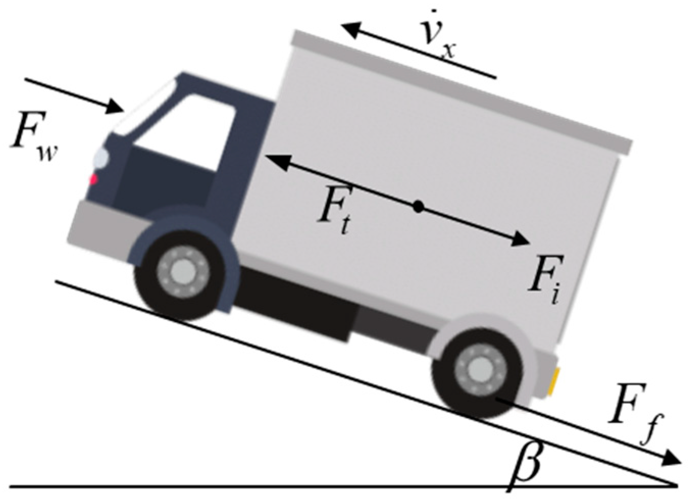
2.1. Vehicle Longitudinal Dynamics Model

Commercial vehicles traveling on the road type are complex and variable; according to the type of slope, they are divided into straight line uphill and downhill conditions, continuous turning uphill and downhill conditions, as well as the two mutually coupled conditions. The road slope type is shown in Figure 2.
As shown in Figure 3, the longitudinal dynamic model of a commercial vehicle on a road with a slope of β degree. The longitudinal dynamic model mainly consists of vehicle driving force, air resistance, rolling resistance, and slope resistance.
For driving force, F t is given as follows:
F t = T t q i g i 0 η r e
For rolling resistance, F f is given as follows:
F f = m t g f cos β
For air resistance, F w is given as follows:
F w = C d A ρ v x 2 2
For road slope resistance, F i is given as follows:
F i = m t g sin β
The expression of the longitudinal dynamic model is shown in Equation (1):
m t v ˙ x = T t q i g i 0 η r e C d A ρ v x 2 2 m t g f cos β m t g sin β
where v ˙ x represents the longitudinal acceleration of the vehicle; m t represents the total mass of commercial vehicles; T t q represents the driving torque of the vehicle; i g represents the transmission ratio of commercial vehicle transmissions; i 0 represents the final transmission ratio of the entire transmission system; η represents transmission efficiency; r e represents the rolling radius of the wheel; C d represents the wind resistance coefficient; A represents the windward area of the vehicle; ρ represents air density; g represents gravitational acceleration; f represents the rolling resistance coefficient of the vehicle; and β represents the slope angle of the road on which the vehicle is traveling.
According to the slope standard in the highway design specifications [22], the value of the road slope is very small. Therefore, cos β 1 , sin β tan β β , and Equation (5) is expressed as follows:
m t v ˙ x = T t q i g i 0 η r e C d A ρ v x 2 2 m t g f m t g β

2.2. Kinematic Model Based on Acceleration Sensor

When the vehicle is driving on a continuous turning uphill and downhill, the longitudinal acceleration is measured by the acceleration sensor, and the relationship between the longitudinal acceleration measurement value and other parameters can be expressed as follows:
a s e n x = v ˙ x v y r z + g sin β
where a s e n x represents the longitudinal acceleration value measured by the acceleration sensor; v y represents the lateral speed of the vehicle; and r z represents the yaw rate.
When a commercial vehicle travels on a longitudinal slope road, Equation (3) can be expressed as follows:
a s e n x = v ˙ x + g sin β

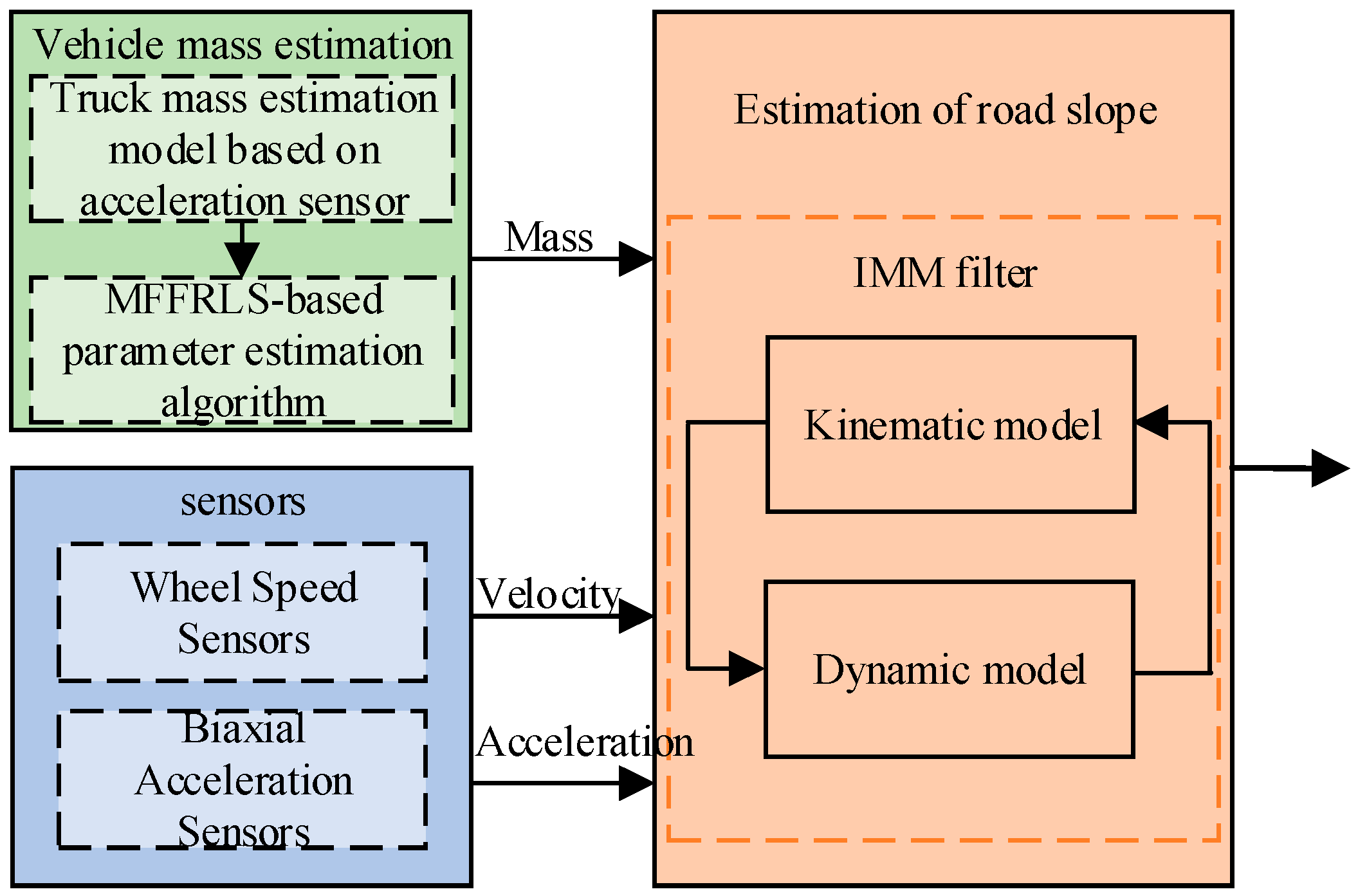
3. Estimation of Commercial Vehicle Mass

The mass estimation method for commercial vehicles was obtained using the joint estimation method of M-estimation and the forgetting factor recursive least squares. Equations (6) and (8) can be combined to obtain the following:
m t a s e n x = T t i g i 0 η r e C d A ρ v x 2 2 m t g f
Equation (9) is converted into the standard equation form of the recursive least squares method as follows:
y = φ T θ + e
In Equation (10), we obtain the following:
y = T t i g i 0 η r e C d A ρ v x 2 2 φ = a s e n x + f g θ = m t
In Equation (11), y represents the output data; φ represents the measurable parameters; θ represents the parameter to be estimated; and e represents Gaussian white noise.
According to [23], it can be seen that the least squares method uses the sum of squares to minimize residuals; thus, the estimation results are more sensitive to sensor outliers. This article introduces the idea of the Huber function into the recursive least squares method to improve the robustness of commercial vehicle mass estimation algorithms and eliminate the impact of sensor abnormal errors.
The standard form of the recursive least squares method based on forgetting factor is as follows:
θ ^ k = θ ^ k 1 + L k ( y k φ k T θ ^ k 1 ) L k = P k 1 φ k T ( λ k + φ k T P k 1 φ k ) 1 P k = ( P k 1 ( I L k φ k T ) / λ k
where P k represents the covariance matrix; L k represents the gain matrix; λ k represents the forgetting factor, mainly used to weaken the impact of historical data on the estimation results; and 0.9 < λ k < 1 .
To address the issue of abnormal errors in sensor measurement data, M-estimation is combined with the forgetting factor recursive least squares to improve the robustness of the algorithm. Therefore, the objective function is defined as follows:
J ( θ k ) = ρ ( r k )
where r k = ( y k φ k T θ k ) , and function ρ can be expressed as follows:
ρ ( r k ) = 0.5 r k 2                             | r k | c         c | r k | 0.5 r k 2       | r k | > c
where c is an adjustable variable, and the derivative of the performance function is as follows:
𝜕 J ( θ k ) 𝜕 θ k = ρ ( r k ) 𝜕 r k 𝜕 x k = 0
We then define ψ k = ρ ( r k ) r k . ψ k is the weight value, and can be expressed as follows:
ψ k = 1                                                     | r k | < c c | r k |                                             | r k | > c
The weight value ψ k is introduced into the forgetting factor recursive least squares method, and its expression is as follows:
θ ^ k = θ ^ k 1 + L k ψ k ( y k φ k T θ ^ k 1 ) L k = P k 1 φ k T ( λ k + φ k T P k 1 φ k ) 1 P k = ( P k 1 ( I ψ k L k φ k T ) / λ k
By introducing a weight value ψ k , when the innovation value r k exceeds the set value, the weight value ψ k is updated to weaken the impact of abnormal measurement data or power fluctuations caused by shifting in the sensor at time k.

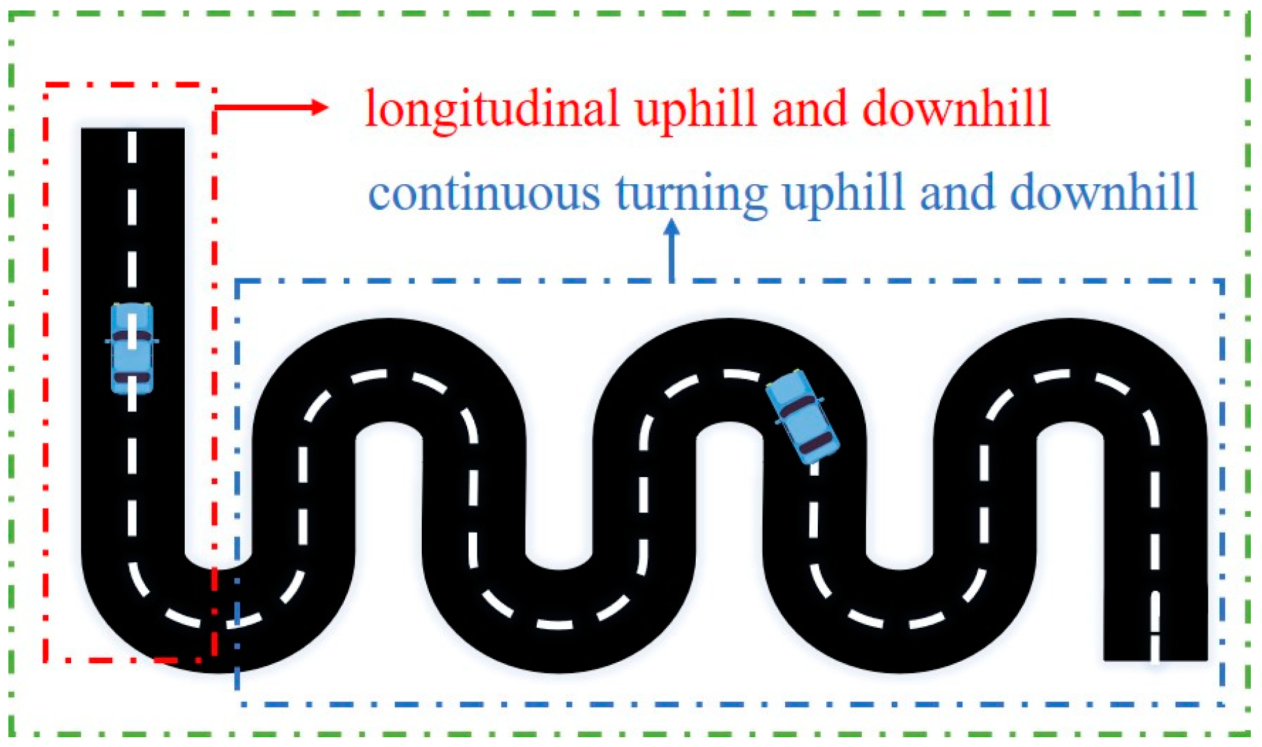
4. Slope Estimation Under Complex Conditions

4.1. Design of State Equations and Observation Equations Under Complex Road Conditions

Commercial vehicles are mainly used for transportation, so the driving conditions are relatively complex, such as winding mountain roads, longitudinal road slopes, continuous turning uphill and downhill, and other roads. The tires of commercial vehicles will generate lateral inertia force and lateral tire force under the working conditions given above. Therefore, when using a longitudinal dynamic model for road slope estimation, the estimated results will deviate. The tire model is used to estimate the lateral force of vehicle tires. Common tire models used for tire force estimation include Magic Tire Model [24], Unitire Model [25], etc. However, commercial vehicles have two different situations, unloaded and loaded, in which parameters such as vehicle mass and center of mass position will change. Therefore, tire models with vehicle mass and center of mass position set as parameters will also change. Moreover, under straight longitudinal slope conditions, model simplification and parameter changes can cause errors in tire models. In summary, considering the issue of model error, an error compensation model based on model error criteria was designed. Based on this, estimation algorithms were used to estimate the slope of commercial vehicles on complex roads.
In order to accurately reflect the changes in the state of commercial vehicles, a dynamic model of commercial vehicles based on time-varying parameters is established:
m t ( v ˙ x v y r z ) = i , j = 1 2 F x i j C d A ρ v x 2 2 m t g f β m t g sin β i , j = 1 2 F x i j = F x f l cos δ f l F y f l sin δ f l + F x f r cos δ f l F y f r sin δ f l + F x r l + F x r r
where F x i j represents the longitudinal force of the tire; F y i j represents the lateral force of the tire; and δ f l represents the front wheel angle.
The longitudinal dynamics model of commercial vehicles only reflects the total driving force of the vehicle’s tires and does not pay attention to the component forces of each tire. Therefore, Equations (1) and (18) are organized as follows:
v ˙ x = T t q i g i 0 η r e m t C d A ρ v x 2 2 m t g f cos β g sin β + v y r z + Δ F F x i j m t T t q i g i 0 η r e m t + Δ F
where Δ F represents the system model error.
Considering the system model error Δ F , the state equation of the state observation system is expressed as follows:
x ˙ ( k ) = f ( x ( k ) , u ( k ) ) + E s ( k )
where the state variable is x ( k ) = [ v x , β 1 ] ; f ( x ( k ) , u ( k ) ) = [ f 1 , f 2 ] T , and f 1 and f 2 can be expressed as follows:
f 1 = T t q i g i 0 η r e m t C d A ρ v x 2 2 m t g f cos β g sin β + v y r z f 2 = 0
In Equation (20), E s ( k ) represents the state error, mainly composed of model error and process noise:
E ( k ) = G ( k ) d ( k ) + w ( k )
In Equation (22), d ( k ) = [ Δ F x f l , Δ F x f r , Δ F y f l , Δ F y f r , Δ F x r l , Δ F x r r ] T ; therefore, the error G ( k ) can be expressed as follows:
G ( k ) = [ cos δ f         cos δ f       sin δ f sin δ f       1         1         0                         0                               0                               0         0         0 ]
The observation equation of the system can be expressed as follows:
z ( k ) = h ( x ( k ) , u ( k ) ) + E o ( k )
where the observed variable is z ( k ) = [ v x , a x ] , h ( x ( k ) , u ( k ) ) = [ h 1 , h 2 ] T , h 1 and h 2 can be expressed as follows:
h 1 = v x h 2 = T t q i g i 0 η r e m t C d A ρ v x 2 2 m t g f cos β g sin β + v y r z
where E o ( k ) represents the observation error, mainly composed of tire force error and measurement noise, which can be expressed as follows:
E o ( k ) = M ( k ) d ( k ) + v ( k )
In Equation (26), the measurement error M ( k ) can be expressed as follows:
M ( k ) = [ 0 0 0 0 0 0 cos δ f cos δ f sin δ f sin δ f 1 1 ]
By using the forward Euler method to discretize Equation (20), the difference equation of the dynamic model of commercial vehicles under continuous turning up- and downhill conditions can be obtained as follows:
v x ( k ) = d t ( T t q i g i 0 η r e m t C d A ρ v x 2 2 m t g f cos β g sin β + v y r z + G 1 d ( k 1 ) ) +                               v x ( k 1 ) β 1 ( k ) = β 1 ( k 1 ) + G 2 d ( k 1 )
When the wheel angle is less than the set threshold and the estimated road slope is greater than the set threshold, the state equation and observation equation in the scenario of continuous turning uphill and downhill are transformed into the state equation and observation equation in the scenario of longitudinal road slopes.

4.2. Error Compensator Design

The presence of a certain error Δ F has been recorded during the turning process and on straight sections with large longitudinal road slopes on mountain roads and continuous turning uphill and downhill. The error Δ F results in the presence of an uncertainty term d ( k ) in the state equation and observation equation, which can affect the estimation of the road slope under complex road conditions. Therefore, the minimum error criterion is used to compensate for the uncertainty term [23].
To minimize the impact of uncertainty on system observations in complex road models, the performance function of the minimum model error compensator is defined as follows:
J d ( k ) = 1   2 ( z ( k ) z ^ ( k ) ) T R 1 ( z ( k ) z ^ ( k ) ) + 1   2 d T ( k ) γ d ( k )
where z ^ ( k ) represents the estimated observation value at time k; R represents measurement noise; and γ represents the semi positive definite error weight matrix. According to Equation (24), the observation equation requires the system state at time k. However, due to the unknown state of the prediction filter based on the minimum model error criterion at time k, the first-order Taylor expansion of Equation (24) yields the following:
z ^ ( k ) = h ( x ^ ( k 1 ) , u ( k ) ) + M d ( k ) + d t 𝜕 h 𝜕 x x ˙ | x = x ( k 1 ) + v ( k ) d t 𝜕 h 𝜕 x x ˙ = d t L G ( h ) d ( k ) + d t L f ( h ) L G ( h ) = 𝜕 h ( x , u ) 𝜕 x G | x = x ( k 1 ) L f ( h ) = 𝜕 h ( x , u ) 𝜕 x f ( x , u )
where 𝜕 h 𝜕 x represents the Jacobian matrix of the observation equation; L G ( h ) represents the first-order Lie derivative of the observation matrix h with respect to matrix G; L f ( h ) represents the first-order Lie derivative of the observation matrix h with respect to the state equation f; and dt represents the sampling time.
The partial derivative of d ( k ) can be calculated through the performance function J [ d ( k ) ] , and according to the minimum principle, its minimum value can be obtained through 𝜕 J [ d ( k ) ] / 𝜕 d ( k ) = 0 . Therefore, in the case of minimizing the performance function, the calculation process of the uncertainty term d ( k ) in the model can be expressed as follows:
d ( k ) = { C ( k ) T R 1 C ( k ) + γ } 1 C ( k ) T R 1 Δ Δ = [ S ( k ) + z ^ ( k ) z ( k ) ] C ( k ) = M ( k ) + d t L G ( h ) S ( k ) = d t L f ( h ) z ^ ( k ) = h ( x ^ ( k 1 ) , u ( k ) )

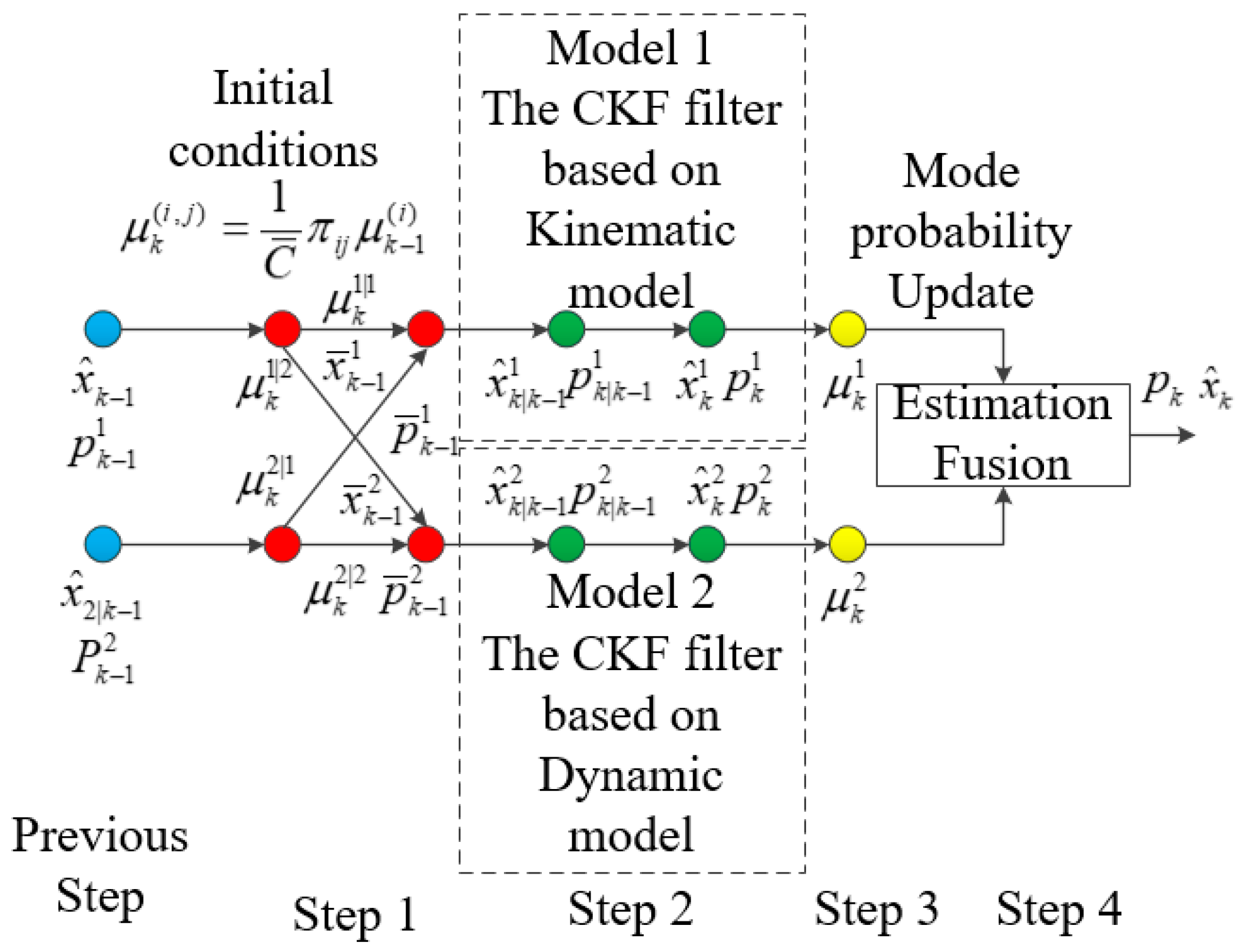
4.3. Interacting Multiple-Model Road Slope Estimation Algorithm

Most existing road slope estimation algorithms are based on longitudinal dynamic or kinematic models for longitudinal road slope estimation. However, for the actual driving conditions of vehicles, in most cases, vehicles are driving on coupling scenarios of longitudinal road slopes and continuous turning uphill and downhill. Therefore, this article proposes an adaptive multi-model fusion strategy for complex working conditions. The overall process of the estimation method is shown in Figure 4. The stochastic process is used to estimate the model probabilities and adjust the weights of the two vehicle models according to the type of slope road. The estimates from each model are then integrated to improve the slope estimation accuracy. Under longitudinal uphill and downhill conditions, the kinematic model is relatively simple, and therefore the kinematic model is appropriate. However, under continuous turning uphill and downhill conditions, the proposed error compensation model has a higher accuracy and is therefore suitable. The IMM-CKF-based slope estimation method can be divided into four parts, which are interacting, filtering, model probability updating, and estimation fusion.
The IMM-CKF (interacting multiple-model–cubature Kalman filter) can be divided into four steps, which are described as follows:
  • Step 1: Interacting
In the first step, the multi-model state values obtained from the estimation of the previous step are multiplied with the mixing weight values of the current step. The mixing weight values can be expressed as follows:
u i j ( k 1 | k 1 ) = p i j u i ( k 1 ) / c j
where u i ( k 1 ) represents the model probability of model in the k − 1 step. The mixing probabilities can be expressed as follows:
c j = i = 1 2 p i j u i ( k 1 )
The model transition of IMM filters between different models is determined by the model transition probability matrix p i j of the Markov process. The model transition probability matrix p i j describes the probability of transitioning from model i to model j. The model transition probability matrix p i j can be expressed as follows:
p i j = 0.98 0.01 0.02 0.99
where i represents model A and j represents model B. The mixed a priori state estimation and covariance for each CKF filter model can be expressed as follows:
x ¯ k 1 | k 1 ( i ) = E ( x k 1 | m k ( i ) Z k 1 ) = i = 1 r x ^ k 1 | k 1 ( i ) μ k 1 | k 1 ( i , j )
p ¯ k 1 | k 1 ( i ) = i = 1 r [ P k 1 | k 1 ( i ) + ( x ^ k 1 | k 1 ( j ) x ¯ k 1 | k 1 ( j ) ) ( x ^ k 1 | k 1 ( j ) x ¯ k 1 | k 1 ( j ) ) T ] μ k 1 | k 1 ( i , j )
  • Step 2: Model-matched filtering
In this step, CKF is used to obtain the states x ^ k | k and covariance P k | k of two models.
The two models should be discretized into the following:
x k = f ( x k 1 , u k 1 ) + w k 1 z k = h ( x k , u k ) + v k
where x k n x is the state of the vehicle at time k; z k n x represents measurement; u k n x represents the input; and w k 1 n x and v k n x denote the independent process and measurement of Gaussian noise sequences assumed to be independent of white noise and with covariances Q k and R k . The overall CKF calculation process can be expressed as follows:
(i).
Time update:
S k 1 | k 1 = S V D ( P k 1 | k 1 ) χ k 1 | k 1 = S k 1 | k 1 ξ + x k 1 | k 1 χ k | k 1 * = f ( χ k 1 | k 1 ) x k | k 1 = 1 m i = 1 m χ i , k | k 1 * P k | k 1 = 1 m i = 1 m χ i , k | k 1 * χ i , k | k 1 * T x k | k 1 x k | k 1 T + Q k
(ii).
Measurement update:
S k | k 1 = S V D ( P k | k 1 ) χ k | k 1 = S k | k 1 ξ + x k | k 1 Z k | k 1 = h ( χ k | k 1 ) z k | k 1 = 1 m i = 1 m Z i , k | k 1 P z z , k | k 1 = 1 m i = 1 m Z i , k | k 1 Z i , k | k 1 T z k | k 1 z k | k 1 T + R k P x z , k | k 1 = 1 m i = 1 m χ i , k | k 1 Z i , k | k 1 T x k | k 1 z k | k 1 T + R k K k = P x z , k | k 1 P z z , k | k 1 1 x k | k = x k | k 1 + K k ( z k z k | k 1 ) P k | k = P k | k 1 K k P z z , k | k 1 K k T
where SVD represents the matrix singular value decomposition method; S represents the square-root of the covariance matrix P; m = 2 n ; ξ = m / 2 [ 1 ] i ; χ i represents the Cubature point, which is generated by the state equations; and Z i represents the Cubature point, which is generated by measurements.
  • Step 3: Model probability update
Under the Gaussian assumption, the likelihood function and model probability of the two models can be expressed, respectively, as follows:
Λ k ( i ) = P ( z ˜ k ( i ) | m k ( i ) , z k 1 ) = 2 π S k ( i ) 1 / 2 exp 1 2 ( z ˜ k ( i ) ) T ( S k ( i ) ) 1 z ˜ k ( i )
μ k ( i ) = P ( m k ( i ) | z k ) = 1 c Λ k ( i ) c ¯ j
c = i = 1 r Λ k ( i ) c ¯ j
where S k ( i ) = H k ( i ) P k | k 1 ( i ) ( H k ( i ) ) T + R k ( i ) ; S k ( i ) denotes the covariance; and c represents the normalization factor.
  • Step 4: Estimation Fusion
The vehicle state estimation and covariance can be obtained by Gaussian mixing equations as shown in Equations (42) and (43).
x ^ k | k = i = 1 r x ^ k ( i ) μ k ( i )
P k | k = i = 1 r [ P k | k ( i ) + ( x ^ k | k x ^ k | k ( i ) ) ( x ^ k | k x ^ k | k ( i ) ) T ] μ k ( i )
where μ k ( i ) represents a weighting of the interaction and the combination of stat estimation.

5. Simulation and Analysis

In order to verify the feasibility and effectiveness of the proposed algorithm, a hardware-in-the-loop (HIL) platform based on Trucksim2020 and Matlab/Simulink2020 is used to analyze and validate the algorithm. The hardware-in-the-loop simulation platform is shown in Figure 5. The real-time controller used in this paper is the MicroAutoBox rapid prototyping controller from dSPACE (Paderborn, Germany). The parameter estimation algorithm using Matlab/Simulink can be downloaded and run in real time on MicroAutoBox. The real-time simulation platform used in this paper is the simulator developed by NI. By downloading the TruckSim vehicle model into the simulator, the vehicle’s running effect can be simulated, and real-time data can be passed to the controller. The specific parameters of the vehicle model are shown in Table 1.

5.1. Introduction of Test Conditions and Initial Value Setting

In order to evaluate the mass estimation stability problem of freight vehicles under different types of acceleration, micro-acceleration and normal acceleration conditions were set up, as shown in Table 2. Under the working condition of micro-acceleration, there is no gear shifting operation for the vehicle. However, under normal acceleration conditions, gear shifting operations exist. The gear shifting operation will lead to fluctuations in power, which in turn affects the accuracy of mass estimation.
In order to evaluate the results of road slope estimation under complex road conditions, complex coupled conditions are set up, which include longitude uphill and downhill and continuous turning uphill and downhill.
The initial value setting for the freight vehicle mass estimation algorithm is as follows: forgetting factor λ k = 0.9995 ; adjustable parameter c = 200 .
The initial value setting for road slope estimation algorithms is as follows: the process noise covariance matrix Q 1 = Q 2 = d i a g ( [ 0.95 , 10 4 ] ) ; the covariance of the measurement noise R 1 = R 2 = d i a g ( [ 10 3 , 10 3 ] ) ; and the chi-square distribution quantile M 1 = 0.02 , M 2 = 4.605 . The weight matrix in the minimum model criterion is as follows:
γ = d i a g ( [ 0.5 10 2 , 0.5 10 2 , 0.5 10 2 , 0.5 10 2 , 0.5 10 2 , 0.5 10 2 ] ) .

5.2. Analysis of Simulation Results

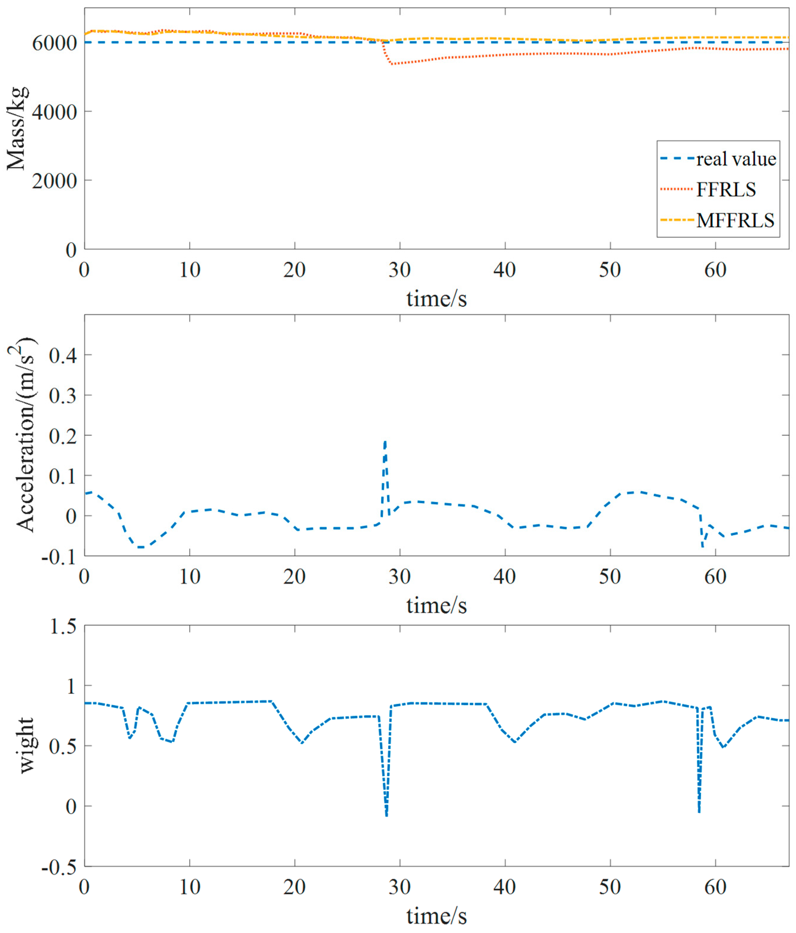
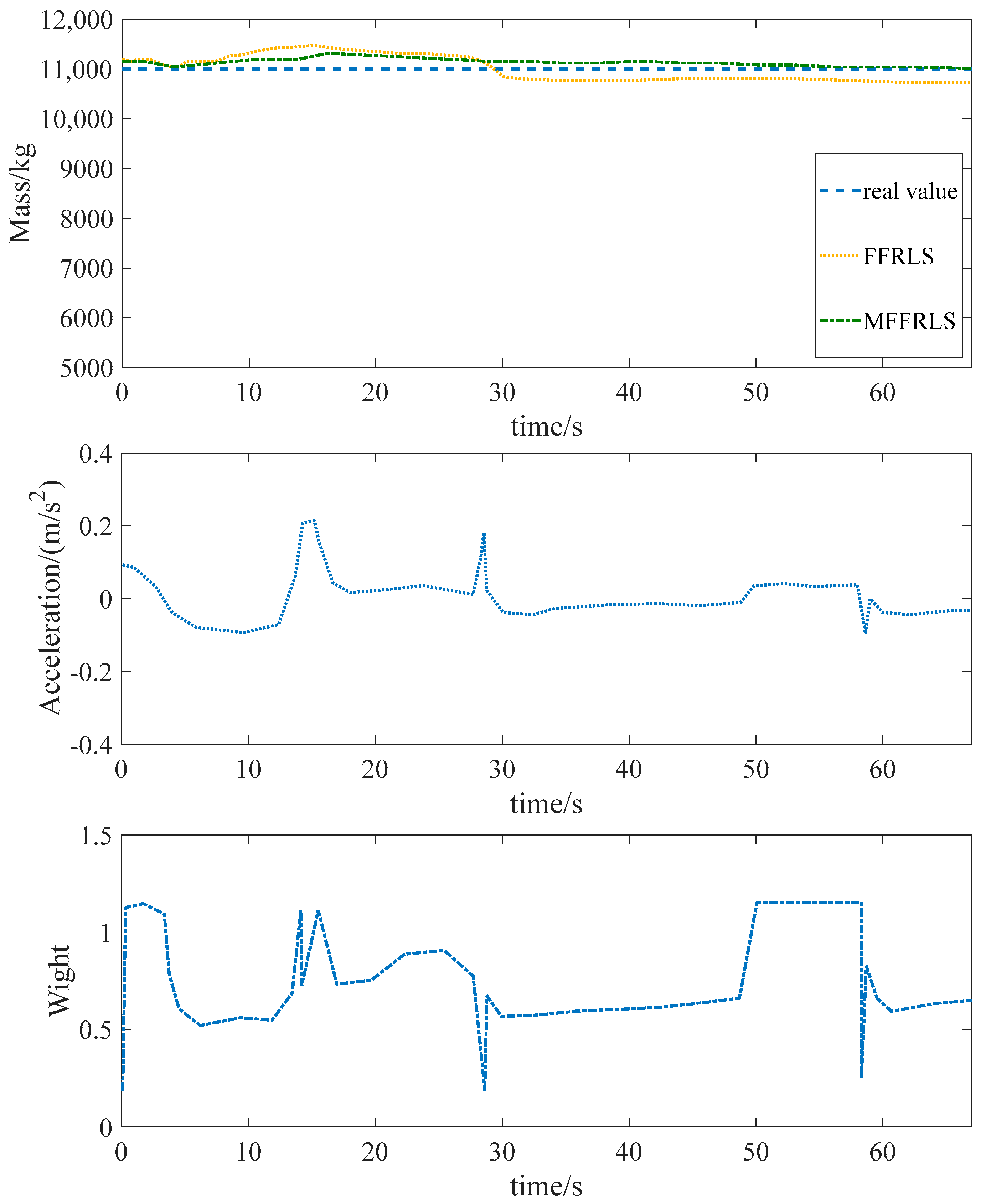
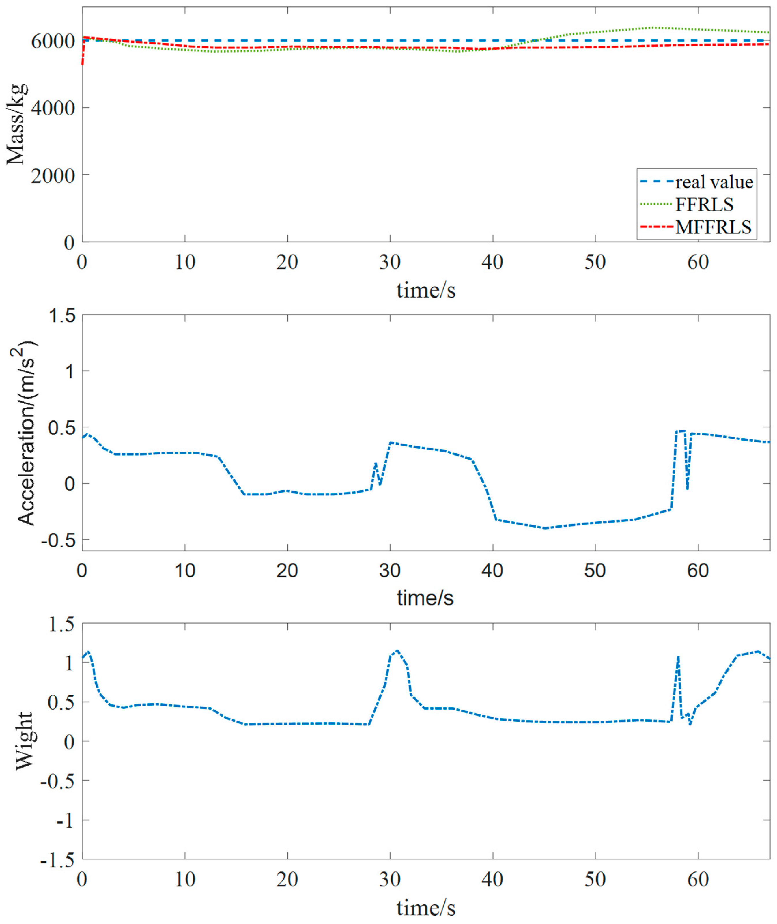
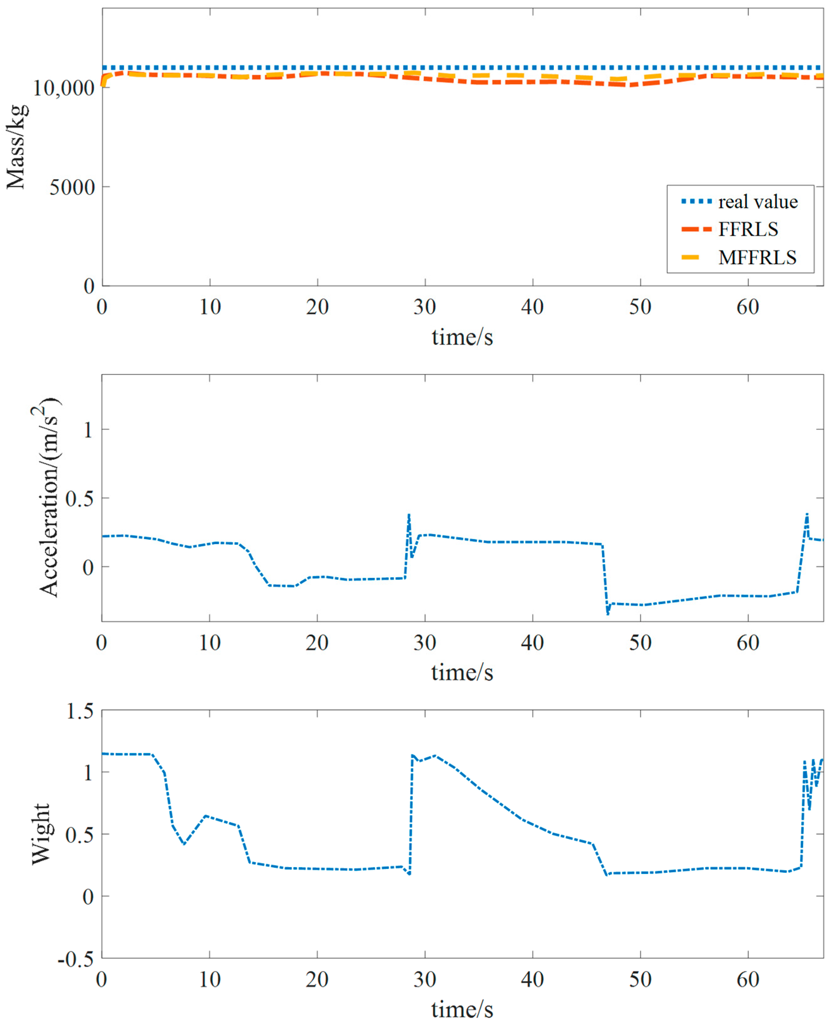
5.2.1. Simulation Test of Mass Estimation Under Different Accelerations

Based on the simulations conducted under micro-acceleration and standard acceleration conditions as outlined in Table 2, the proposed vehicle mass estimation algorithm is compared with the FFRLS algorithm. The results pertaining to unloaded and loaded trucks with a load of 5000 kg are presented in Figure 6 and Figure 7, respectively.
From Figure 6, it is evident that when mass estimation is performed using the FFRLS algorithm, the estimated mass undergoes significant fluctuations and deviates from the true value in the presence of abnormal error effects on the sensor measurement variable around 28 s. As the FFRLS algorithm iterates, the mass estimation results gradually converge towards the true value due to the influence of the forgetting factor that is inherent in the algorithm. However, when the sensor measurement variable is again subjected to an anomalous error at approximately 57 s, the quality estimates do not exhibit significant jittering as the algorithm becomes less sensitive to new data due to the increasing number of iterations and the effect of the forgetting factor.
In contrast, the mass estimation based on the MFFRLS algorithm demonstrates robustness against abnormal errors affecting the sensor measurement variables. In this case, when new information introduces an abrupt change, the weight values are attenuated by the Huber function, ensuring that the estimate from the previous moment, which is deemed more accurate, is trusted during the mass estimation process. As depicted in Figure 6, in the presence of abnormal disturbances in the sensor measurement variables, the weight values are assigned close to zero, thereby enhancing the robustness of the freight vehicle mass estimation algorithm. Similarly, in Figure 7, the algorithm exhibits the same characteristics as observed in Figure 6 when the sensor is impacted by anomalous errors.
The experimental data under standard acceleration conditions are shown in Figure 8 and Figure 9. As can be seen in Figure 8, the mass estimation results do not produce large jitter due to the strong excitation when the sensor measurements are affected by anomalous errors. At around 28, 38, and 57 s, when the truck is shifting gears, the mass estimation based on the MFFRLS algorithm does not have any jitter or sudden change. The robustness of the algorithm can also be seen in Figure 9.

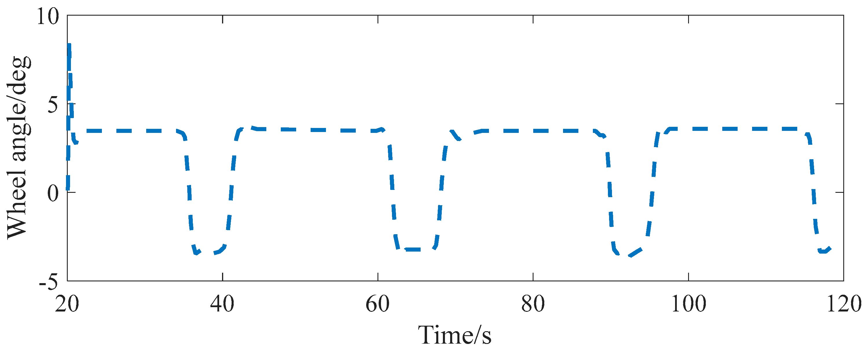
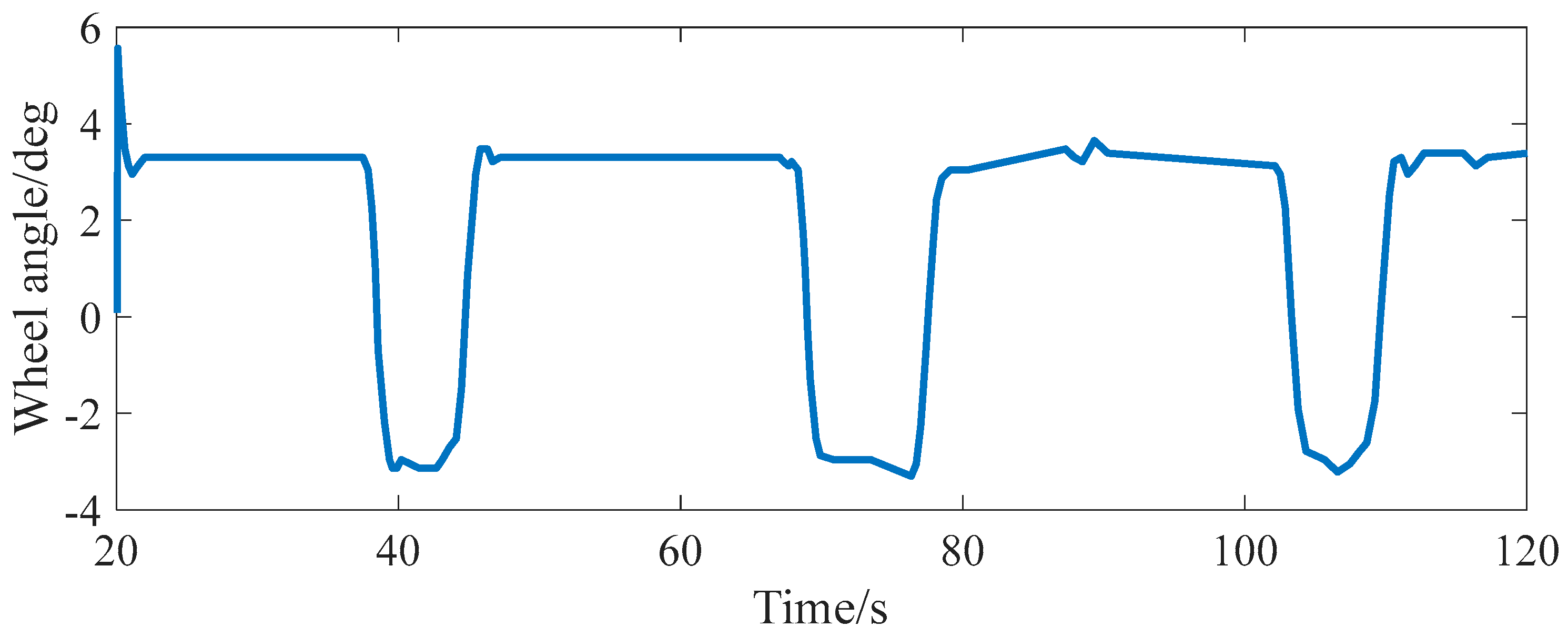
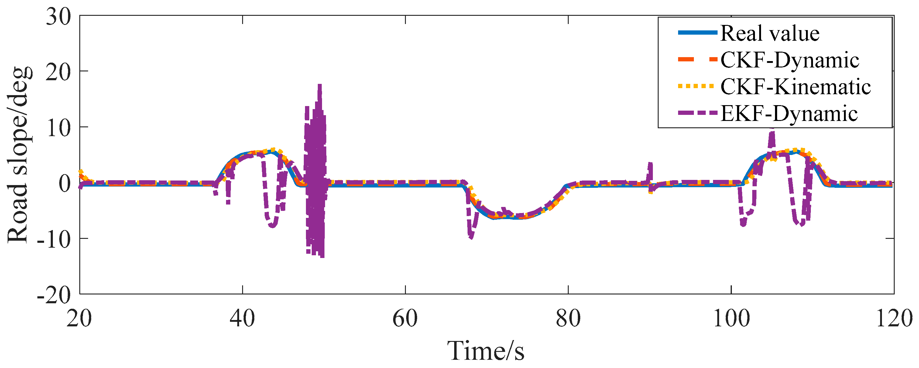
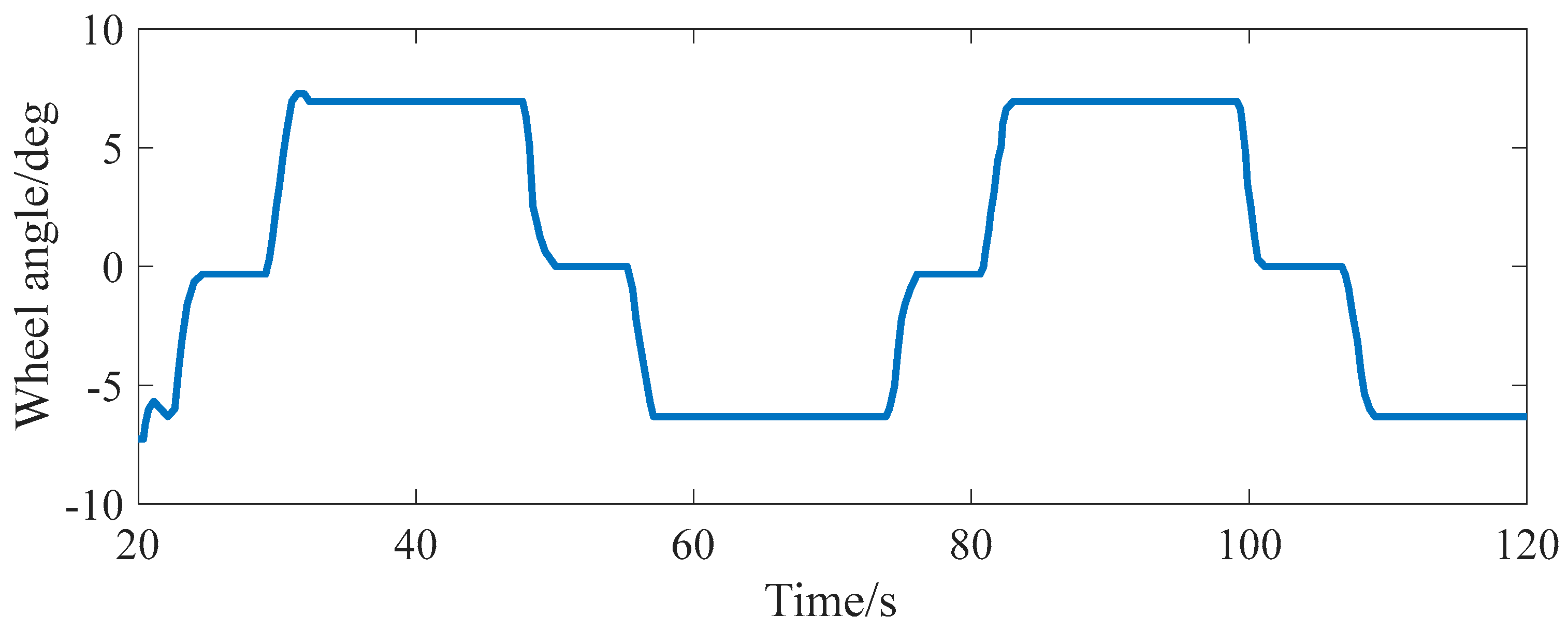
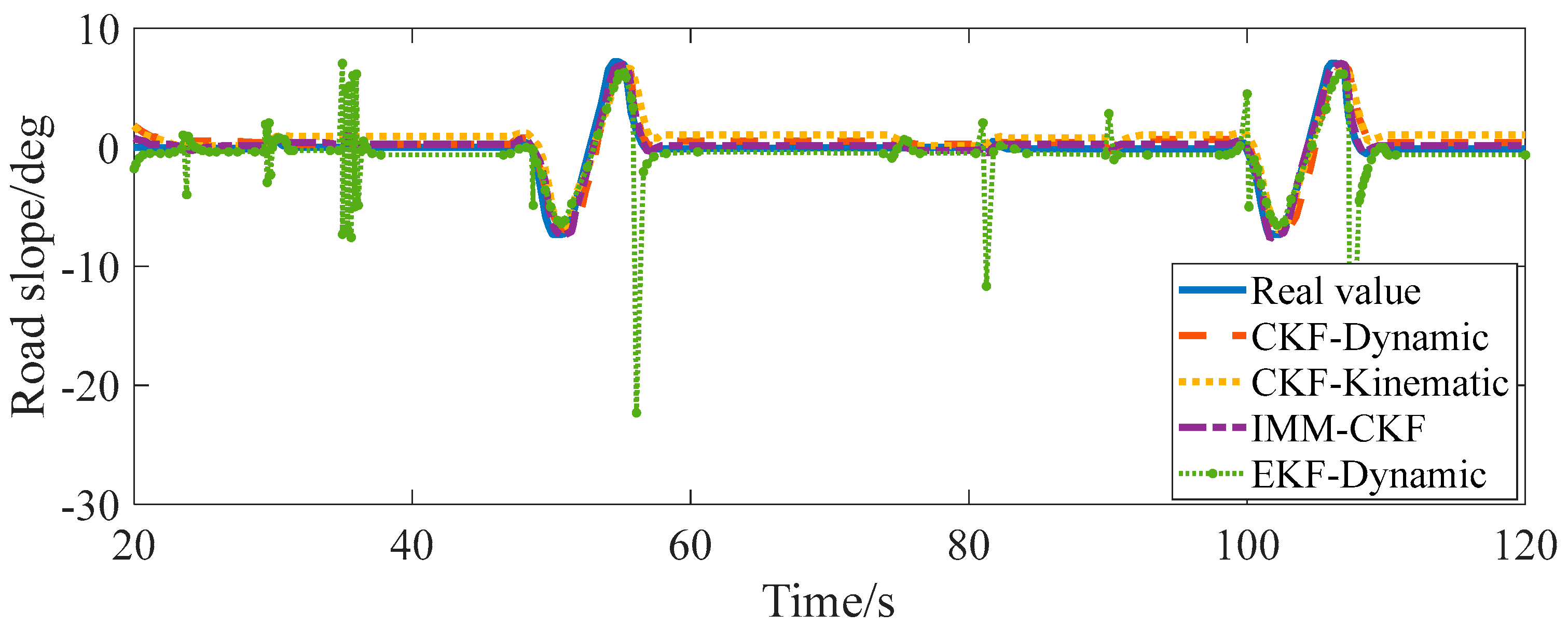
5.2.2. Simulation Experiment of Slope Estimation Under Complex Coupled Road Conditions

In this part, the results of the CKF slope estimation algorithm based on the kinematic model and on the kinetic model are firstly compared under continuous turning uphill and downhill conditions. This comparison of simulation results under different loads and the comparison of simulations under the influence of abnormal errors of sensor measurement variables are performed, respectively. Figure 10 shows the wheel steering angle data when the vehicle is under no load. As can be seen from Figure 11, under the continuous turning uphill and downhill conditions, the CKF (cubature Kalman filter) algorithm based on the compensated dynamic model can accurately estimate the road slope in real-time, and the estimation results are superior to those of other algorithms.
For the kinematic model, the slope estimation results obtained by using the CKF algorithm show a certain forward offset. This is because the kinematic model is designed for straight-line conditions. When the vehicle turns horizontally, there is a component of the center of mass along the horizontal axis, which leads to estimation deviation.
Regarding the dynamic model, the error of slope estimation using the EKF (extended Kalman filter) algorithm is relatively large. This is because the EKF handles non-linear problems by means of first-order Taylor expansion, ignoring the higher-order terms of the model, thus resulting in relatively large errors.
In terms of noise interference, steady noise interference was applied at two time periods, 32–37 s and 90–95 s, respectively. The EKF road slope estimation results based on the kinematic model showed frequent jitter, while the CKF based on the kinematic model had a strong suppression effect on the noise disturbance.
Figure 12 shows the wheel angle data at a vehicle load of 5000 kg. Figure 13 shows the road slope estimation data at a load of 5000 kg. The error of the road slope estimation based on the kinematic model increases, while the road slope estimation of the CKF algorithm based on the kinetic model remains close to the real road slope value.
For the complex coupled road conditions consisting of straight longitudinal ramps and continuous turning up and down slopes, the analysis is carried out from the following three aspects: analysis of the road slope estimation results under the complex coupled road; analysis of the road slope estimation results under the noise interference; and analysis of the weight allocation of the fusion strategy under the complex coupled road.
Figure 14 shows the wheel-turning angle data. It can be seen that in the four time periods of 25–30 s, 50–54 s, 76–80 s, and 100–106 s, the vehicle is in a straight-line traveling state after turning. In the other time periods, the vehicle is in the turning uphill and downhill condition. The results of slope estimation are shown in Figure 15. Under the continuous turning uphill and downhill conditions, the estimation accuracy of the CKF (cubature Kalman filter) algorithm based on the dynamic model is superior to that based on the kinematic model. However, under straight-line conditions (25–30 s, 50–54 s, 76–80 s, 100–106 s), the CKF algorithm based on the kinematic model shows better accuracy in slope estimation than the one based on the dynamic model. Moreover, the IMM-CKF (interacting multiple-model–cubature Kalman filter) algorithm proposed in this paper enables accurate estimation under straight-road conditions, continuous turning uphill and downhill conditions, as well as their coupled conditions.
In the analysis of the estimation results under noise interference, the IMM-CKF algorithm proposed in this paper can effectively suppress the noise interference.
Each model probability calculated by the IMM algorithm is shown in Figure 16. The model probabilities imply that different models are suitable for different road slope conditions. The kinematic model probability is much higher than the kinetic model probability in the straight-line slope condition. Based on this result, it can be seen that the kinetic model is more suitable for straight-line slope conditions compared to the kinetic model. By comparison, it can be seen that in the turning uphill and downhill, the kinematic model probability is much higher than the kinematic model probability [26,27]. It means that the kinetic model is more suitable for continuous turning uphill and downhill conditions.

5.3. Analysis of Error Results

In order to verify the accuracy of the proposed method, the Root Mean Square Error (RMSE) is used for evaluation.
R M S E ( x ) = k = 1 n ( x ^ ( k | k ) x i , t r u e ) 2 n
where x ^ ( k | k ) represents the estimation result of the proposed algorithm and x i , t r u e is the true value.
Table 3 and Table 4, respectively, present the comparison of the Root Mean Square Error (RMSE) index for vehicle mass estimation under the conditions of slight acceleration and normal acceleration and deceleration. When the freight vehicle undergoes slight acceleration without gear shifting, and is affected by abnormal sensor errors, the precision of the MFFRLS (Modified Forgetting Factor Recursive Least Squares) algorithm is significantly superior to that of the FFRLS (Forgetting Factor Recursive Least Squares) algorithm, and it also exhibits better robustness.
For a freight vehicle carrying goods under normal acceleration and deceleration driving conditions, due to the presence of gear shifting behavior and the influence of abnormal sensor errors, there is not much difference between the mass estimation results of MFFRLS and FFRLS. Through the comparison of the mass estimation results during slight acceleration and normal acceleration and deceleration driving, it can be seen that under slight acceleration, for different cargo loads, the RMSE of the mass estimation by the MFFRLS algorithm remains stable at around 170 kg, while the RMSE of the mass estimation by the FFRLS algorithm fluctuates around 250 kg. The main reason for this situation is the influence of abnormal sensor errors, which are inevitable during the actual transportation process of the freight vehicle.
Regarding normal acceleration and deceleration, as the load increases, the value of the RMSE shows an increasing trend. When the load is 5000 kg, the RMSE values of the FFRLS and MFFRLS algorithms reach 406 kg and 345 kg, respectively. The main reasons for this increasing trend of estimation error are composed of two parts: The first part is that the parameters in the longitudinal dynamics are all set as fixed values, and as the load increases, the parameters of the longitudinal dynamics model will change accordingly. The second part is due to the gear shifting operation during the normal acceleration process, which causes power fluctuations during the gear shifting process. Among them, the second part is the main reason for the increasing RMSE of the mass estimation.
Based on the above analysis, it can be concluded that the mass estimation results obtained by the proposed MFFRLS algorithm have the smallest error and the best stability under slight acceleration driving conditions.
As shown in Table 5, when the truck travels on a complex coupled road with different loads, even under the influence of abnormal errors in sensor measurement variables, the proposed fusion strategy improves the road slope estimation results by about 3% compared to the estimation results of the other two methods under different loading conditions. The results show that the proposed algorithm can effectively solve the road slope problem under complex coupled road conditions and has good estimation accuracy and robustness.

6. Conclusions

In order to address the issues of mass estimation and slope estimation of vehicles when driving under complex working conditions such as on winding mountain roads and continuous turning uphill and downhill roads, a joint estimation strategy is proposed.
(1)
By combining the M-estimation method with the recursive least squares method with a forgetting factor, the mass estimation of trucks is realized. Under both the micro-acceleration and normal acceleration working conditions, the estimation accuracy of the MFFRLS (M-estimation-based Forgetting Factor Recursive Least Squares) is superior to that of the FFRLS (Forgetting Factor Recursive Least Squares) algorithm, and it has strong anti-interference characteristics.
(2)
Aiming at the complex situation that combines the working conditions of straight uphill and downhill and continuous turning uphill and downhill, a road slope estimation algorithm based on the IMM-CKF is proposed. Under different load conditions, compared with the estimation algorithm based on a single model, the accuracy of the estimation results of the proposed algorithm is improved by 3%, and it has good robustness.
Finally, the joint estimation algorithm proposed in this paper is verified by using a hardware-in-the-loop test platform. The joint estimation algorithm proposed in this paper can accurately estimate the vehicle state parameters under the conditions of continuous turning uphill and downhill, straight uphill and downhill, as well as complex coupling working conditions, providing a reference for the safety research of trucks. In the next stage, the verification on a real vehicle will be our research objective.

Funding

This research was funded by the Henan Science and Technology Research Project (242102520046), the Henan University Young Backbone Teachers Plan (2021GGJS180).

Data Availability Statement

The data that support the fundings of this study are available from the corresponding author upon reasonable request.

Conflicts of Interest

The authors declare no conflicts of interest.

Nomenclature

β road slope angle (deg)
v ˙ x longitudinal acceleration of the vehicle (m/s2)
m t total mass of commercial vehicles (kg)
T t q driving torque of the vehicle (N·m)
i g transmission ratio of commercial vehicle transmissions
i 0 final transmission ratio of the entire transmission system
η transmission efficiency (%)
r e rolling radius of the wheel (m)
C d wind resistance coefficient
A windward area of the vehicle (m2)
ρ air density (kg/m3)
g gravitational acceleration (m/s2)
f rolling resistance coefficient of the vehicle
R e wheel radius (m)
a s e n x longitudinal acceleration value measured by the acceleration sensor (m/s2)
v y lateral speed of the vehicle (m/s)
r z yaw rate (rad/s)
F x i j longitudinal force of the tire (N)
F y i j lateral force of the tire (N)
δ f l front wheel angle (deg)

References

  1. Shi, J.; Lu, T.; Li, X.; Zhang, J. Self-adaptive slope gearshift strategy for automatic transmission vehicles. Trans. Chin. Soc. Agric. Mach. 2011, 42, 1–7. [Google Scholar]
  2. Yin, Z.; Dai, Q.; Guo, H.; Chen, H.; Chao, L. Estimation road slope and longitudinal velocity for four-wheel drive vehicle. IFAC-PapersOnLine 2018, 51, 72–577. [Google Scholar] [CrossRef]
  3. Xu, S.; Li, S.E.; Cheng, B.; Li, K. Instantaneous feedback control for a fuel-prioritized vehicle cruising system on highways with a varying slope. IEEE Trans. Intell. Transp. Syst. 2016, 18, 1210–1220. [Google Scholar] [CrossRef]
  4. Li, S.E.; Guo, Q.; Xu, S.; Duan, J.; Li, S.; Li, C.; Su, K. Performance enhanced predictive control for adaptive cruise control system considering road elevation information. IEEE Trans. Intell. Veh. 2017, 2, 150–160. [Google Scholar] [CrossRef]
  5. Jin, M.; Zhao, J.; Jin, J.; Yu, G.; Li, W. The adaptive Kalman filter based on fuzzy logic for inertial motion capture system. Measurement 2014, 49, 196–204. [Google Scholar] [CrossRef]
  6. Zhang, X.; Xu, L.; Li, J.; Ouyang, M. Real-time estimation of vehicle mass and road grade based on multi-sensor data fusion. In Proceedings of the 2013 IEEE Vehicle Power and Propulsion Conference (VPPC), Beijing, China, 15–18 October 2013. [Google Scholar]
  7. Apriliani, E.; Nurhadi, H. Ensemble and Fuzzy Kalman Filter for position estimation of an autonomous underwater vehicle based on dynamical system of AUV motion. Expert Syst. Appl. 2017, 68, 29–35. [Google Scholar]
  8. Johansson, K. Road Slope Estimation with Standard Truck Sensors; KTH: Stockholm, Sweden, 2005. [Google Scholar]
  9. Hao, S.; Luo, P.; Xi, J. Estimation of vehicle mass and road slope based on steady-state Kalman filter. In Proceedings of the 2017 IEEE International Conference on Unmanned Systems (ICUS), Beijing, China, 27–29 October 2017. [Google Scholar]
  10. Massel, T.; Ding, E.; Arndt, M. Investigation of different techniques for determining the road uphill gradient and the pitch angle of vehicles. In Proceedings of the 2004 American Control Conference, Boston, MA, USA, 30 June–2 July 2004; Volume 3. [Google Scholar]
  11. McIntyre, M.L.; Ghotikar, T.J.; Vahidi, A.; Song, X.; Dawson, D.M. A two-stage Lyapunov-based estimator for estimation of vehicle mass and road grade. IEEE Trans. Veh. Technol. 2009, 58, 3177–3185. [Google Scholar] [CrossRef]
  12. Lei, Y.; Fu, Y.; Liu, K.; Zeng, H.; Zhang, Y. Vehicle Mass and Road Grade Estimation Based on Extended Kalman Filter. Trans. Chin. Soc. Agric. Mach. 2014, 45, 9–14. [Google Scholar]
  13. Lingman, P.; Schmidtbauer, B. Road slope and vehicle mass estimation using Kalman filtering. Veh. Syst. Dyn. 2002, 37 (Suppl. 1), 12–23. [Google Scholar] [CrossRef]
  14. Bar-Shalom, Y.; Li, X.R.; Kirubarajan, T. Estimation with Applications to Tracking and Navigation: Theory Algorithms and Software; John Wiley & Sons: Hoboken, NJ, USA, 2004. [Google Scholar]
  15. Tsunashima, H.; Murakami, M.; Miyataa, J. Vehicle and road state estimation using interacting multiple model approach. Veh. Syst. Dyn. 2006, 44 (Suppl. 1), 750–758. [Google Scholar] [CrossRef]
  16. Blom, H.; Bar-Shalom, Y. The interacting multiple model algorithm for systems with Markovian switching coefficients. IEEE Trans. Autom. Control. 1988, 33, 780–783. [Google Scholar] [CrossRef]
  17. Barrios, C.; Himberg, H.; Motai, Y.; Sadek, A. Multiple model framework of adaptive extended Kalman filtering for predicting vehicle location. In Proceedings of the 2006 IEEE Intelligent Transportation Systems Conference, Toronto, ON, Canada, 17–20 September 2006. [Google Scholar]
  18. Ndjeng, A.N.; Glaser, S.; Gruyer, D. A multiple model localization system for outdoor vehicles. In Proceedings of the 2007 IEEE Intelligent Vehicles Symposium, Istanbul, Turkey, 13–15 June 2007. [Google Scholar]
  19. Dawood, M.; Cappelle, C.; El Najjar, M.E.; Khalil, M.; Pomorski, D. Vehicle geo-localization based on IMM-UKF data fusion using a GPS receiver, a video camera and a 3D city model. In Proceedings of the 2011 IEEE Intelligent Vehicles Symposium (IV), Baden, Germany, 5–9 June 2011. [Google Scholar]
  20. Zhang, Z.; Zheng, L.; Li, Y.; Yu, Y. Research on intelligent vehicle target state tracking based on robust adaptive sckf. J. Mech. Eng. 2021, 57, 181–193. [Google Scholar]
  21. He, Y.; Yan, X.; Chu, D.; Lu, X.-Y.; Wu, C. A probabilistic prediction model for the safety assessment of HDVs under complex driving environments. IEEE Trans. Intell. Transp. Syst. 2016, 18, 858–868. [Google Scholar] [CrossRef]
  22. Li, E.; He, W.; Yu, H.; Xi, J. Model-based embedded road grade estimation using quaternion unscented kalman filter. IEEE Trans. Veh. Technol. 2022, 71, 3704–3714. [Google Scholar] [CrossRef]
  23. Liu, W.; He, H.; Sun, F. Vehicle state estimation based on minimum model error criterion combining with extended Kalman filter. J. Frankl. Inst. 2016, 353, 834–856. [Google Scholar] [CrossRef]
  24. Pacejka, H.B.; Bakker, E. The magic formula tyre model. Veh. Syst. Dyn. 1992, 21, 1–18. [Google Scholar] [CrossRef]
  25. Guo, K.; Lu, D.; Chen, S.-K.; Lin, W.C.; Lu, X.-P. The UniTire model: A nonlinear and non-steady-state tyre model for vehicle dynamics simulation. Veh. Syst. Dyn. 2005, 43, 341–358. [Google Scholar] [CrossRef]
  26. Jo, K.; Chu, K.; Sunwoo, M. Interacting multiple model filter-based sensor fusion of GPS with in-vehicle sensors for real-time vehicle positioning. IEEE Trans. Intell. Transp. Syst. 2011, 13, 329–343. [Google Scholar] [CrossRef]
  27. Toledo-Moreo, R.; Zamora-Izquierdo, M.A.; Ubeda-Minarro, B.; Gómez-Skarmeta, A.F. High-integrity IMM-EKF-based road vehicle navigation with low-cost GPS/SBAS/INS. IEEE Trans. Intell. Transp. Syst. 2007, 8, 491–511. [Google Scholar] [CrossRef]
Figure 1. Overall architecture of the IMM-based slope estimation system.
Wevj 16 00172 g001
Figure 2. Schematic diagram of road slope types.
Wevj 16 00172 g002
Figure 3. Vehicle longitudinal dynamics model.
Wevj 16 00172 g003
Figure 4. Process of the IMM-CKF.
Wevj 16 00172 g004
Figure 5. Hardware-in-the-loop test platform.
Wevj 16 00172 g005
Figure 6. Mass estimation data for an unloaded vehicle under micro-acceleration conditions.
Wevj 16 00172 g006
Figure 7. Mass estimation data for a loaded vehicle under micro-acceleration conditions.
Wevj 16 00172 g007
Figure 8. Mass estimation results for the unloaded vehicle under normal acceleration and deceleration conditions.
Wevj 16 00172 g008
Figure 9. Mass estimation results for the loaded vehicle under normal acceleration and deceleration conditions.
Wevj 16 00172 g009
Figure 10. Wheel-turning angle data under no load conditions.
Wevj 16 00172 g010
Figure 11. Results of slope estimation under no load conditions.
Wevj 16 00172 g011
Figure 12. Wheel-turning angle data under load conditions.
Wevj 16 00172 g012
Figure 13. Results of slope estimation under load conditions.
Wevj 16 00172 g013
Figure 14. Wheel-turning angle data.
Wevj 16 00172 g014
Figure 15. Results of slope estimation.
Wevj 16 00172 g015
Figure 16. Model probability calculated by the IMM algorithm.
Wevj 16 00172 g016
Table 1. Main parameters of the vehicle model.
Parameter NameValue
Vehicle mass m t 6000 kg
Effective rolling radius of the tire r e / m 0.6 m
Transmission efficiency η 0.92
Air density ρ 1.206 kg/m3
Windward area A0.8 m2
Drag coefficient C d 7
Table 2. Working condition settings for mass estimation.
Test ConditionsLoad Mass
Micro-acceleration0 kg
Micro-acceleration5000 kg
Normal acceleration0 kg
Normal acceleration5000 kg
Table 3. Comparison of Root Mean Square Error (RMSE) indicators for vehicle mass estimation under micro-acceleration conditions.
ParameterLoad Mass (kg)FFRLSMFFRLS
Vehicle mass0269.72167.34
3000222.12175.37
5000259.16169.75
Table 4. Comparison of Root Mean Square Error (RMSE) indicators for vehicle mass estimation under standard acceleration conditions.
ParameterLoad Mass (kg)FFRLSMFFRLS
Vehicle mass0269.72159.28
3000390.11311.78
5000406.57345.67
Table 5. Comparison of RMSE indicators for road slope estimation.
ParameterLoad MassDynamic ModelKinematic ModelIMM_CKF
Slope00.3312.5470.328
30000.3482.3870.331
50000.3092.6480.301
Disclaimer/Publisher’s Note: The statements, opinions and data contained in all publications are solely those of the individual author(s) and contributor(s) and not of MDPI and/or the editor(s). MDPI and/or the editor(s) disclaim responsibility for any injury to people or property resulting from any ideas, methods, instructions or products referred to in the content.

