Multi-UAV Delivery Path Optimization Based on Fuzzy C-Means Clustering Algorithm Based on Annealing Genetic Algorithm and Improved Hopfield Neural Network

Abstract

This study develops an MTSP model for multi-UAV delivery optimization from a central hub, proposing a hybrid algorithm that integrates genetic simulated annealing-enhanced clustering with an improved Hopfield neural network to minimize the total flight distance. The proposed methodology initially employs an enhanced fuzzy C-means clustering technique integrated with genetic simulated annealing (GSA) to effectively partition the MTSP formulation into multiple discrete traveling salesman problem (TSP) instances. The subsequent phase implements an enhanced Hopfield neural network (HNN) architecture incorporating three key modifications: data normalization procedures, adaptive step-size control mechanisms, and simulated annealing integration, collectively improving the TSP solution quality and computational efficiency. The proposed algorithm’s effectiveness is validated through comprehensive case studies, demonstrating significant performance improvements in the computational efficiency and solution quality compared to conventional methods. The results show that during clustering, the improved clustering algorithm is more stable in its clustering effect. With regard to path optimization, the improved neural network algorithm has a higher computational efficiency and makes it easier to obtain the global optimal solution. Compared with the genetic algorithm and ant colony algorithm, its iteration times, path length, and delivery time are reduced to varying degrees. To sum up, the hybrid optimization algorithm has obvious advantages for solving a multi-UAV collaborative distribution path optimization problem.

1. Introduction

At present, unmanned aerial vehicles (UAVs) are widely used in the military, agricultural, commercial, and civil fields, and have become a research hotspot. UAVs have obvious advantages in maneuverability, speed, positioning accuracy, and stability, and can be applied to practical distribution problems for meeting customer demand requirements. Regarding UAV distribution, it essentially belongs to the path optimization problem of UAVs. The path optimization problem has always been a research hotspot due to its NP-difficult characteristics, such as the following.

Liu et al. [1] studied the distribution routing problem of cold chain logistics and proposed an improved genetic algorithm. With the wide application of UAVs, UAV path optimization has attracted widespread attention from scholars. To fully leverage the operational advantages of UAV-based delivery systems, Chen et al. [2] investigated a time-constrained electric vehicle–UAV collaborative routing optimization with partial charging strategies, and developed a hybrid metaheuristic that integrates a large neighborhood search with variable neighborhood descent to address the problem’s distinctive characteristics. Wang, J.Q. et al. [3] studied the reconnaissance path problem of a UAV and designed a cross-entropy algorithm to solve it. Fu, Z.T. et al. [4] studied the patrol path optimization of multi-UAV dangerous goods container yards, and constructed a 01 integer programming model with the shortest total flight distance of all UAVs as the goal and the maximum range of UAVs as the constraint, and designed a full-scanning simulated annealing algorithm. Liu, W.B. et al. [5] studied the multi-traveling salesman route-planning problem of multi-UAV collaborative searches and multi-targets. In order to complete the task as quickly as possible, a multi-traveling salesman model was established, and an optimization algorithm composed of a clustering algorithm and a genetic algorithm was designed. Cao, Z.K. [6] studied the multi-UAV land survey route-planning and -scheduling problem. Mao, H.T. et al. [7] studied the UAV reconnaissance path planning problem considering relay charging, established a mixed-integer programming model that aims at the smallest number of UAVs and shortest overall reconnaissance time, and designed an improved ant colony algorithm. Wang et al. [8] investigated optimal flight path planning in dynamic and complex environments, and developed a novel hybrid algorithm (HIDOA-SOS) through the integration of an enhanced wild dog optimization algorithm (HIDOA) with symbiotic organism search (SOS) techniques. Hu et al. [9] introduced an enhanced sand cat swarm optimization algorithm (LSCSO) for UAV path planning, which incorporates learning mechanisms inspired by sand cats’ behavioral patterns. The proposed algorithm integrates an innovative position update strategy into the conventional sand cat optimization framework, effectively balancing population diversity preservation and convergence acceleration throughout the optimization process. Wang et al. [10] investigated optimal flight path planning in constrained environments, where conventional algorithms have demonstrated limited effectiveness. To address these computational challenges, the authors developed a novel hybrid optimization framework, termed PESSA (Parallel Enhanced Swarm Search Algorithm). Ait-Saadi et al. [11] developed an enhanced metaheuristic framework, the Chaotic Cauchy Opposition-Based African Vulture Optimization Algorithm (CCO-AVOA), specifically designed for three-dimensional UAV path planning optimization challenges. Van et al. [12] introduced an innovative Fermat–Weber Location-Based Particle Swarm Optimization (FWL-PSO) algorithm, which incorporates Fermat–Weber optimality principles to identify the optimal solutions for multi-UAV cooperative path planning challenges.

In the existing research, scholars usually transform the UAV distribution routing problem into the famous traveling salesman problem. The application of a Hopfield neural network to this problem started with Hopfield and Tan [13]. On the one hand, this neural network has the inherent advantages of parallel computation and fault tolerance; on the other hand, a Hopfield network is unrobust, and the initial conditions of a network seriously affect the calculation results, and may still not obtain a feasible solution. This is mainly because the core of a Hopfield network is the gradient descent method, which means that a change in neurons always leads to a decrease in network energy when calculating the energy function and, finally, the network energy may fall into a local minimum or infeasible solution, and the search efficiency is low, so it cannot solve optimization problems efficiently and accurately. In order to make up for the shortcomings of Hopfield neural networks, many scholars have improved the Hopfield neural network from different aspects and have applied it to solve different problems. Some examples follow.

When Chen Xiao et al. [14] studied the traveling salesman problem (TSP), they adopted the method of fixing the travel starting point on the basis of a Hopfield neural network, which reduced the number of neurons, that is, it reduced the unnecessary appearance of equivalent solutions in the solution process. Dang Jianwu et al. [15] established the neural network calculation energy function and iterative formula for each problem, and proposed an intelligent HNN optimization method. Wang Chao et al. [16] improved the HNN by optimizing the energy function of the constraints, which has the advantage of fast convergence speed, and does not easily fall into invalid solutions or easy-to-obtain suboptimal solutions. Yan Chen et al. [17] developed an advanced optimization framework that integrated an enhanced energy function (IEF) with transient chaotic neural network (TCNN) mechanisms to address the local optima convergence limitations of conventional neural networks for solving NP-class optimization problems. Jolai et al. [18] enhanced the algorithm’s global search capabilities through the synergistic integration of the Hopfield neural network (HNN) architecture with advanced data transformation techniques (DTTs). An et al. [19] improved the energy function of the HNN to solve the TSP. Lin et al. [20] proposed a method of applying genetic operators to an HNN to ensure the global search ability of the network. At the same time, a dynamic learning rate was introduced into the HNN to accelerate the convergence speed of the neural network. Guo Zhonghua et al. [21] aimed at the problem that a Hopfield neural network is prone to invalid solutions and poor convergence performance when solving TSPs, and proposed a method that strictly restricts the “row” and “column” terms of the energy function and uses soft-limiting functions to improve the neuron dynamic equation. Tarkov [22] introduced a novel neural network-based optimization framework (NWTA) for traveling salesman problem (TSP) solutions, combining enhanced winner-take-all (WTA) deep learning mechanisms with 2 opt optimization techniques to improve the Hopfield recurrent neural network performance. Kai et al. [23] developed an advanced Hopfield neural network architecture specifically designed to address the minimum-cost optimization challenges incorporating time-delay constraints in ad hoc network environments. Hu et al. [24] introduced an Accelerated Augmented Lagrangian Hopfield Neural Network (AALHNN) framework for TSP optimization, effectively overcoming the limitations of traditional penalty-based Lagrange multiplier methods while ensuring reliable solution quality and computational efficiency. Dutta [25] designed a hybrid algorithm of an HNN and SA to solve the TSP. Comert et al. [26] developed a hybrid optimization framework combining K-Means and K-Medoids clustering techniques with a Hopfield neural network (HNN) architecture to address large-scale TSP challenges. This methodology initially partitions the problem space into optimized clusters, followed by HNN-based path optimization within each cluster to ensure computational efficiency and solution quality. Almuhanna et al. [27] introduced an innovative hybrid optimization framework integrating genetic algorithm (GA) mechanisms with a Hopfield neural network (HNN) architecture for enhanced TSP solution efficiency and accuracy. Li et al. [28] developed a novel fractional-order memristive Hopfield neural network (FMHNN) architecture, integrating fractional calculus principles with memristive devices to achieve enhanced system characteristics, including long-term memory retention and complex chaotic dynamics, resulting in superior TSP optimization performance through accelerated convergence rates and reduced solution path lengths. The relevant literature on improving HNNs to solve TSPs are shown in

Table 1. HNN improvement strategy.

Author	Year	Literature	Improved Energy Function	Improvement Step Size	Other Improvements
Chen Xiao	1996	Literature [14]	-	-	Adopt a fixed travel starting point and reduce the number of neurons.
Dang Jianwu	1997	Literature [15]	-	-	Change progress and column constraints.
Wang Chao	2001	Literature [16]	Optimization constraints	-	-
Yan Chen	2006	Literature [17]	Aiyer improved energy function is adopted	-	-
Jolai	2010	Literature [18]	-	-	Data Transformation Technology (DTT).
An	2011	Literature [19]	Optimize energy term	-	-
Lin	2014	Literature [20]	-	Dynamic step size	Combined with genetic algorithm.
Guo Zhonghua	2014	Literature [21]	The energy function "row" and "column" items are strictly constrained	-	Improvement of neuron dynamic equation using soft-limiting function.
Tarkov	2015	Literature [22]	-	-	Deep learning (WTA) and 2 opt optimization methods.
Kai	2020	Literature [23]	Optimize energy term	-	Adopt a fixed travel starting point and reduce the number of neurons.
Hu	2022	Literature [24]	-	-	Constraints are multiplied by a Lagrange multiplier and an augmented Lagrange multiplier, respectively.
Dutta	2022	Literature [25]	-	-	Combined with SA algorithm.
Comert	2022	Literature [26]	-	-	Hybrid algorithm of K-Means and K-Medoids algorithms and HNN.
Almuhanna	2024	Literature [27]	-	-	Combined with genetic algorithm.
Li	2024	Literature [28]	Combining fractional calculus and memristors	Piecewise dynamic step size	-

.

Aiming at the multi-UAV path optimization problem with a certain scale in this paper, the single algorithm still has limitations in dealing with this problem. In order to overcome the above problems, this paper proposes a hybrid optimization algorithm based on an SA-GA-FCM algorithm and improved HNN. Through a multi-level optimization framework and dynamic collaboration mechanism, this algorithm combines the global search ability of an SA-GA-FCM with the local optimization ability of an improved HNN, which significantly improves the performance of the path optimization problem. Specifically, the SA-GA-FCM algorithm uses the sudden jump characteristics of simulated annealing, the population evolution mechanism of a genetic algorithm, and the spatial partitioning ability of fuzzy clustering to quickly explore the solution space and generate high-quality initial solutions. This enhanced HNN incorporates an adaptive step-size adjustment, data transformation techniques, and simulated annealing integration to improve the solution quality while ensuring algorithmic convergence and optimization capability.

The proposed hybrid algorithm demonstrates three key innovations:

• Multi-algorithm fusion: by combining the advantages of an SA, GA, and FCM and an improved HNN, a dynamic balance between the global search and local optimization is achieved.
• Fuzzy clustering guidance: the FCM is used to fuzzy divide the problem space, and the algorithm is guided to search in key areas to reduce the computational complexity.
• Dynamic collaboration mechanism: through the dynamic collaboration mechanism, the SA-GA-FCM and improved HNN can give full play to their respective advantages at different stages and significantly improve the solution efficiency.

2. Modeling the MTSP of Multi-UAV Collaborative Distribution

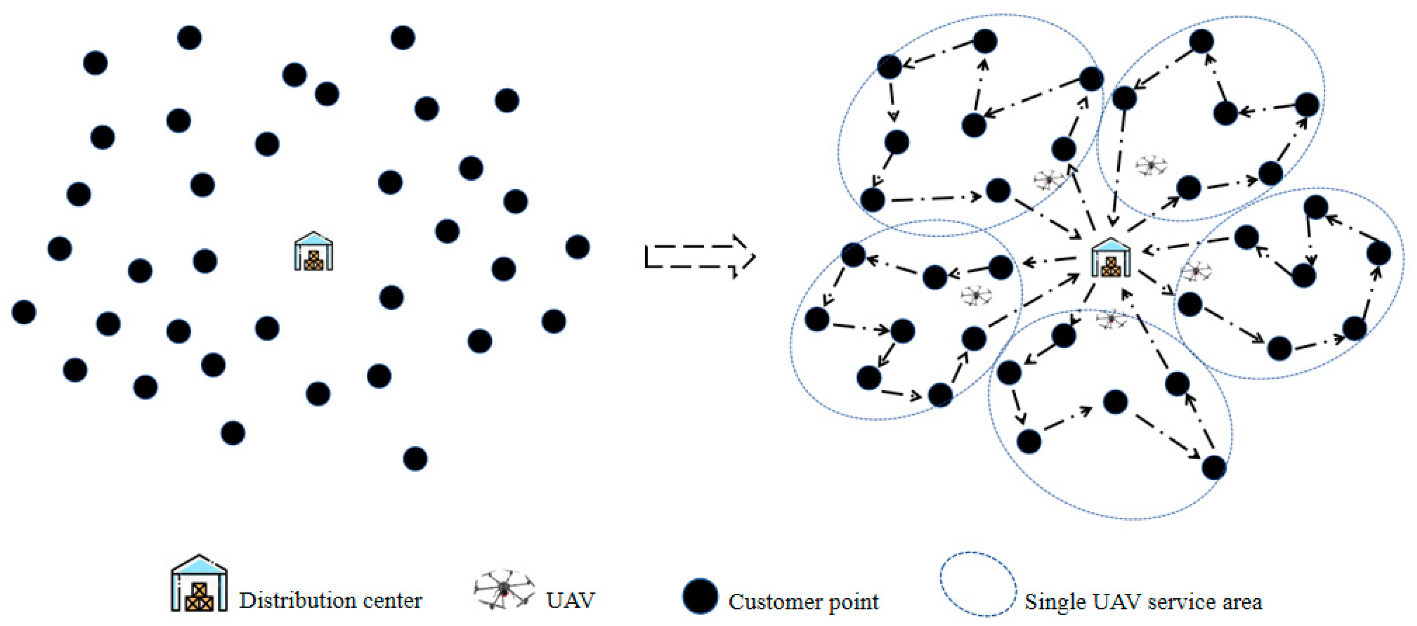
2.1. Problem Description

Assume that there is a distribution center in a certain area, and there are multiple UAVs of the same type in the distribution center to provide UAV distribution services for customers living nearby. Given the constraint that individual customer demands remain within the UAVs’ maximum payload capacity, the system partitions customer nodes into geographically optimized clusters through distance-based clustering analysis. Each UAV is subsequently assigned to service its designated cluster, completing delivery operations before returning to the central distribution facility. Figure 1 is a schematic diagram of a UAV delivery process.

The problem assumes the following:

(1)

The demand and coordinates of each customer are known;

(2)

The speed of each UAV is the same and constant, regardless of the influence of weather on the UAV;

(3)

There is only one distribution center in an area;

(4)

Each customer can be served once and only by one UAV;

(5)

The take-off and landing time of UAVs and the time to serve customers are not considered.

2.2. Mathematical Model

The MTSP is defined by a directed graph G = (V, A), where V is a finite non-empty set of n vertices, A is a set of edges represented by pairs of vertices in V, and the symbol definition is shown in

Table 2. Parameter and variable symbol definition.

Name	Symbols	Definition
Parameter	$i$, $j$	Customer nodes on path, $i,j\in V=\left\{1,2,\dots ,n\right\}$
	$\left(i,j\right)$	Arc segment, $\left(i,j\right)\in A$
	$d_{ij}$	The distance between customer i and customer j
	$q_i$	Quantity demanded by customer i
	$S_i$	The total number of customers, i, served when the UAV arrives at customer i
	$u$	UAV serial number, $u\in m$
	$L_u$	UAV u flight distance
	$L$	The maximum flight distance of the UAV
	T	The time when the UAV serves the last customer
	$Q$	Maximum load capacity of UAV
	$v$	Flight speed of UAVs
	$t_u$	Flight time of UAV u
Decision variables	$x_{ij}^u$	Equal to 1 when UAV u passes i and j, otherwise 0
	$x_{ij}$	When the UAV passes through the arc segment (i, j) $x_{ij}$ is 1, otherwise 0

.

According to the assumptions, the model is established as follows:

$$\min [\max (L_1,L_2,\dots ,L_m)]$$

(1)

$$L_u={\displaystyle \sum _{i=1}^n{\displaystyle \sum _{j=1}^n{d}_{ij}{x}_{ij}^u}},u=1,2,\dots ,m$$

(2)

$$t_u={\displaystyle \frac{L_u}{v}},u=1,2,\dots m$$

(3)

$$\max (L_u)\le L,u=1,2,\dots m$$

(4)

$$\max (t_u)\le T,u=1,2,\dots m$$

(5)

$${\displaystyle \sum _{i=1}^n{\displaystyle \sum _{j=i+1}^{n-1}{q}_i{x}_{ij}^u}}\le Q,u=1,2,\dots m$$

(6)

$${\displaystyle \sum _{j=1}^n{x}_{0j}=m}$$

(7)

$${\displaystyle \sum _{j=1}^n{x}_{j0}}=m$$

(8)

$${\displaystyle \sum _{i=1}^n{x}_{ij}=}1,j=2,\cdot \cdot \cdot ,n$$

(9)

$${\displaystyle \sum _{j=1}^n{x}_{ij}=1,i=2,\cdot \cdot \cdot ,n}$$

(10)

$$S_i-S_j+(n-m)x_{ij}\le n-m-1$$

(11)

$$1\le i\ne j\le n$$

(12)

$$x_{ij}\in \left\{0,1\right\},\forall (i,j)\in A$$

(13)

Equation (1) represents the minimization of the maximal aggregate traversal distance across the fleet of UAVs.

Equation (2) represents the total distance flown by a UAV during the delivery process.

Equation (3) represents the time spent by a UAV flying during the delivery process.

Equation (4) indicates that because a UAV is limited by its own power, there is an upper limit for its flight distance, that is, the maximum flight distance.

Equation (5) indicates that there is also a time limit for customers to receive service. Here, a value is specified, and a UAV can only reach the customer point within this time range, that is, the UAV has the constraint of maximum flight time.

Equation (6) indicates that due to its own performance limitations and the load constraint of a UAV, the total load capacity cannot exceed the maximum load capacity.

Equations (7) and (8) specify that the entire cohort of m UAVs is initialized to embark from the distribution hub, with the operational capability to successfully complete their navigation cycle by returning to the originating depot.

Equations (9) and (10) establish that each customer node receives singular service visitation, ensuring exclusive UAV assignments and eliminating redundant coverage of service locations.

Equation (11) prevents the formation of any route that does not contain UAVs, that is, UAVs must exist in the formed path.

Equation (12) imposes a cardinality constraint on the total number of serviceable customer nodes within the network.

Equation (13) defines a binary decision variable, where the solution space is constrained to [0, 1] integer values.

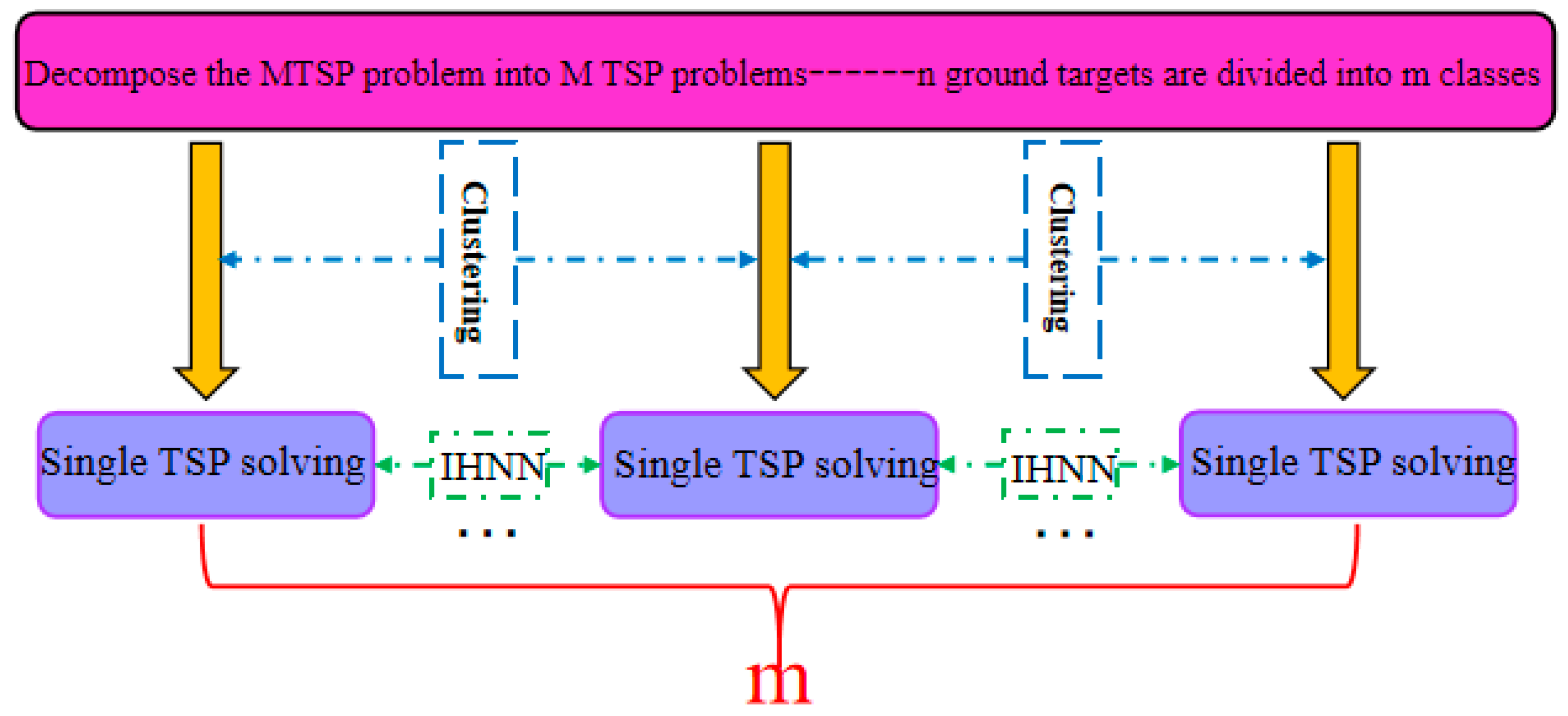
3. Hybrid Optimization Algorithm for Solving MTSP

The proposed solution for the multi-UAV TSP, illustrated in Figure 2, consists of two key components: (1) the decomposition of the MTSP into m TSP instances through a hybrid fuzzy C-means and annealing genetic algorithm, and (2) the optimization of each TSP using an enhanced Hopfield neural network incorporating data normalization, adaptive step factors, and simulated annealing for the shortest-path solutions.

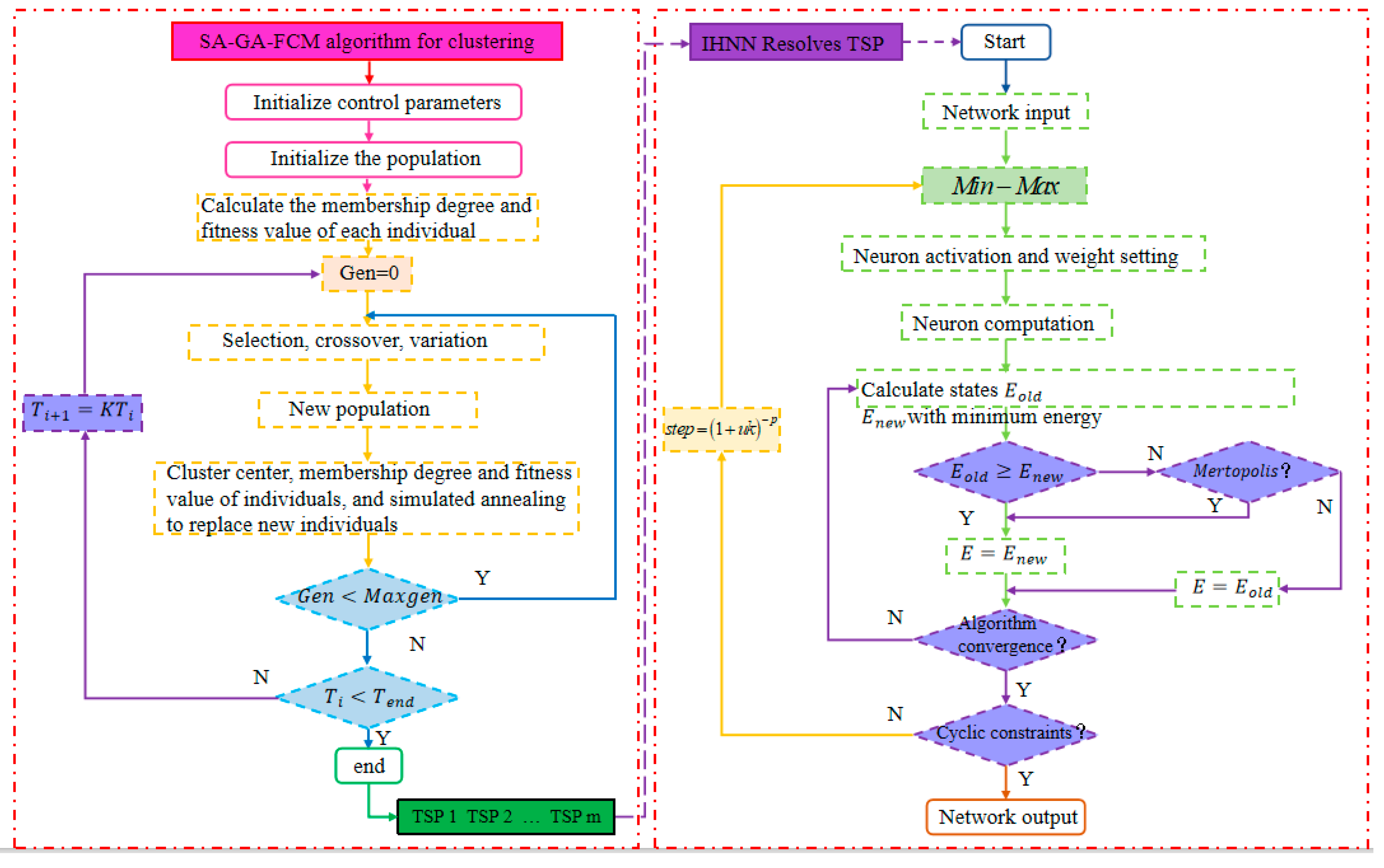
3.1. Fuzzy C-Means Clustering Algorithm Based on Annealing Genetic Algorithm (SA-GA-FCM)

A fuzzy C-means clustering (FCM) algorithm is a clustering algorithm that determines the degree of membership of each data point belonging to a certain cluster [29]. Let $X=\left\{x_1,x_2,\dots ,x_n\right\}$ be the data samples, the number be $n$, $c\left(2\le c\le n\right)$ means that the data samples are divided into $c$ classes, and $\left\{S_1,S_2,\dots ,S_c\right\}$ means the corresponding subsets of $c$. If $V=\left\{v_1,v_2,\dots ,v_c\right\}$ is represented as the clustering center of subset $c$ and $u_{ik}$ is the membership degree of sample $x_i$ to class $S_k$, then the client point function $J_b$ and the corresponding constraints are represented as follows:

$$\begin{array}{l}\left\{\begin{array}{l}{J}_b(U,v)={\displaystyle \sum _{i=1}^n{\displaystyle \sum _{k=1}^c{({\mu }_{ik})}^b{(d_{ik})}^2}}\\ {\displaystyle \sum _{\mathrm{i}=1}^{\mathrm{c}}{u}_{ik}=1,0<{\displaystyle \sum _{k=1}^n{u}_{ik}<1,1\le b\le \infty }}\\ d_{ik}=d\left(x_i-v_k\right)=\sqrt{{\displaystyle \sum _{j=1}^m{\left(x_{ij}-v_{kj}\right)}^2}}\end{array}\right.\end{array}$$

(14)

where $d_{ik}$ is expressed as the distance between the i-th sample and the k-th center point, m is the number of sample features, and b is the weighting parameter.

The calculation of the sample membership degree ${\mu }_{ik}$ and clustering center $v_{ij}$ is expressed as follows:

$$u_{ik}={\displaystyle \frac{1}{{\displaystyle \sum _{j=1}^c{\left(\frac{d_{ik}}{d_{lk}}\right)}^{\frac{2}{b-1}}}}}$$

(15)

$$v_{ij}={\displaystyle \frac{{\displaystyle \sum _{k=1}^n{\left({\mu }_{ik}\right)}^b{x}_{kj}}}{{\displaystyle \sum _{k=1}^n{\left({\mu }_{ik}\right)}^b}}}$$

(16)

Equations (15) and (16) are used to repeatedly calculate and modify the cluster center and membership degree. Upon algorithm convergence, the theoretical framework yields both the cluster centroids and their associated membership degrees, thereby completing the fuzzy clustering process. Although FCM has high service efficiency, its service is limited to a local area, and it has high requirements for the initial value of the central point. The improper selection of the initial values may lead to convergence at the local optima.

Therefore, a simulated annealing and genetic algorithm combined with FCM are used for the cluster analysis. In terms of service ability, the genetic algorithm has a strong global service ability. Compared with the genetic algorithm, the simulated annealing algorithm has a better local service ability, but its overall service ability is weaker. However, this does not mean that the simulated annealing algorithm easily falls into the local optimum, but it may be difficult to provide service in the most ideal area, thus affecting the overall operation efficiency of the simulated annealing algorithm. Both features complement each other. If they are combined, they can give full play to their respective advantages, which makes the performance of the new global service algorithm more excellent [30]. The specific steps of the algorithm are as follows:

• Denote $S$ as the individual size of the population; $M$ as the maximum number of evolution; and $P_c$, $P_m$ represent the probability of crossover and mutation, respectively. $T_0$ and $T_{end}$ represent the initial temperature and the termination temperature when the annealing operation is performed, respectively, and $k$ represents the cooling coefficient of the temperature.
• Randomly calculate the number of clustering centers c; at this time, an initial population is generated, denoted as C. Using Formulas (15) and (16), the membership degree of each sample in the cluster center and the fitness value $f_i,i=1,2,\dots ,S$ of each individual in the population are calculated.
• Set the loop parameters so that GEN = 0.
• Perform a genetic operation on population C, that is, selection, crossover, and mutation, and new individuals will be generated at this time. In the same step ②, calculate the clustering center of the new individuals, the membership degree of the samples at this time, and the fitness value $f^{’}$ of each individual in the new population. If $f_i^{’}>f_i$, the old individual is abandoned and the newly generated individual is accepted; otherwise, the probability $P=\exp \left(\left(f_i-f_i^{’}\right)/T\right)$ is calculated to accept the new individual with a probability of $P$.
• If Gen < M, let Gen = Gen + 1, and return to step 4 to continue the cycle; otherwise, proceed directly to step ⑥.
• If $T_i<T_{end}$, it means that the algorithm ended successfully, and the global optimal solution is output at this time; otherwise, the cooling operation is performed according to the annealing algorithm $T_{i+1}=k{T}_i$, and return to step ③ to continue the cycle.

3.2. Improved Hopfield Neural Network Algorithm (IHNN)

A continuous Hopfield neural network architecture is implemented through the interconnection of the fundamental electronic circuit components [31]. The Figure 3 is a neuron circuit schematic diagram of a continuous Hopfield neural network. There is a feedback connection from the input to output. Under the excitation of the input, there will be constant state changes.

Each neuron within this architecture exhibits a continuous output response, i.e., $v_i=f_i\left(u_i\right)$, where $v_i$, $u_i$ represent the output and input voltages of the i-th neuron, respectively.

For an N-node continuous Hopfield neural network model, the temporal evolution of the neuronal state variables is described by the following system of nonlinear differential equations:

$$\left\{\begin{array}{l}{C}_i{\displaystyle \frac{d{u}_i}{dt}}={\displaystyle \sum _{j=1}^N{T}_{ij}{v}_j-\frac{u_i}{R_i}+I_i}\\ v_i=f_i\left(u_i\right),i=1,2,3,\dots ,N\end{array}\right.$$

(17)

The connection weight $W_{xi,yj}$ between neurons is

$$\begin{array}{l}{W}_{xi,yj}=-A{\delta }_{xy}\left(1-{\delta }_{ij}\right)-B{\delta }_{ij}\left(1-{\delta }_{xy}\right)-\\ C-D{d}_{xy}\left({\delta }_{j,i+1}+{\delta }_{j,i-1}\right)\end{array}$$

(18)

The bias current is

$$I_{xi}=CN$$

(19)

$${\delta }_{ij}=\left\{\begin{array}{l}1\begin{array}{ccc}& & i=j\end{array}\\ 0\begin{array}{ccc}& & i\ne j\end{array}\end{array}\right.$$

(20)

The input state update equation is

$$U_{xi}\left(t+1\right)=U_{xi}\left(t\right)+{\displaystyle \frac{d{U}_{xi}}{dt}}\cdot step$$

(21)

The updated expression of the output state is

$$V_{xi}\left(t\right)={\displaystyle \frac{1}{2}}\left[1+\tanh \left({\displaystyle \frac{U_{xi}\left(t\right)}{U_0}}\right)\right]$$

(22)

The energy function when solving the TSP is defined as

$$\begin{array}{l}E={\displaystyle \frac{A}{2}}{\displaystyle \sum _{x=1}^N{\displaystyle \sum _{i=1}^N{\displaystyle \sum _j^N{V}_{xi}{V}_{xj}}}}+{\displaystyle \frac{B}{2}}{\displaystyle \sum _{i=1}^N{\displaystyle \sum _{x=1}^N{\displaystyle \sum _j^N{V}_{xi}{V}_{yi}}}}+\\ {\displaystyle \frac{C}{2}}{\left({\displaystyle \sum _{x=1}^N{\displaystyle \sum _{i=1}^N{V}_{xi}-N}}\right)}^2+{\displaystyle \frac{D}{2}}{\displaystyle \sum _{x=1}^N{\displaystyle \sum _y^N{\displaystyle \sum _i^N{d}_{xy}{V}_{xi}}}}\left(V_{y,i+1}+V_{y,i-1}\right)\end{array}$$

(23)

A, B, C and D are the weights; $d_{xy}$ represents the distance between $x$ and $y$; the first three terms are the constraint terms of the problem; and the last term is the optimization customer point term. The improved energy function is as follows:

$$\begin{array}{l}E={\displaystyle \frac{A}{2}}{{\displaystyle \sum _{x=1}^N\left({\displaystyle \sum _{i=1}^N{V}_{xi}-1}\right)}}^2+{\displaystyle \frac{A}{2}}{{\displaystyle \sum _{i=1}^N\left({\displaystyle \sum _{x=1}^N{V}_{xi}-1}\right)}}^2+\\ {\displaystyle \frac{D}{2}}{\displaystyle \sum _{x=1}^N{\displaystyle \sum _{y=1}^N{\displaystyle \sum _{i=1}^N{G}_{xy}{V}_{xi}{V}_{y,i+1}}}}\end{array}$$

(24)

The corresponding dynamic equation is as follows:

$$\begin{array}{l}{\displaystyle \frac{d{U}_{xi}}{dt}}=-{\displaystyle \frac{\partial E}{\partial V_{xi}}}=-A\left({\displaystyle \sum _{i=1}^N{V}_{xi}-1}\right)-A\left({\displaystyle \sum _{y=1}^N{V}_{yi}-1}\right)-\\ D{\displaystyle \sum _{y=1}^N{G}_{xy}{V}_{y,i+1}}\end{array}$$

(25)

3.2.1. Data Normalization

Data normalization involves linearly transforming raw data to a standardized range of [0–1] through scaling operations. Eliminate the unit limit of the data, and convert the dimensional data into dimensionless data, which facilitates the comparison and common processing of data in different units or of different magnitudes. In this paper, a min-max normalization [32] is used to preprocess the data, and its conversion function is as follows.

The sequence $x_1,x_2,\dots ,x_n$ is transformed

$$V_i={\displaystyle \frac{x_i-\underset{1\le j\le n}{\min }\left\{x_j\right\}}{\underset{1\le j\le n}{\max }\left\{x_j\right\}-\underset{1\le j\le n}{\min }\left\{x_j\right\}}}$$

(26)

The generated new sequence $V_1,V_2,\dots ,V_n\in [0,1]$ has no dimension. Applying it to the neural network can not only better process the data in the next step, but also speed up the convergence of the training network and ensure the reliability of the results.

3.2.2. The Introduction of Dynamic Step Size

The neural network chooses a fixed step size when learning, and its value is often difficult to choose. Excessively large step sizes accelerate the initial optimization but may prematurely converge the model to suboptimal solutions, either local or global. However, if the learning is carried out in large steps all the time, the weight update will be too large, which will make the performance of the model oscillate during the training period, resulting in large fluctuations, and even the value of the loss function will hover around the minimum value, which will always make it difficult to achieve the optimum. If the step size is too small, the algorithm may converge slowly or never reach convergence. Therefore, the concept of step size attenuation is introduced, that is, a larger step size is used for model optimization in the early stages of training. As the number of iterations increases, the step size will gradually decrease, ensuring that there will be no large fluctuations in the later stages of model training, thus coming closer to the optimal solution; see Figure 4 for the schematic diagram. Take the step size as

$$step={\left(1+uk\right)}^{-p}$$

(27)

u takes a positive number less than or close to 1, k is the number of iterations, and p is a constant greater than zero.

3.2.3. Application of Simulated Annealing Algorithm

The simulated annealing algorithm, inspired by thermodynamic annealing processes, employs temperature-dependent probabilistic transitions to identify the global optima, thereby mitigating the local optima convergence limitations inherent in Hopfield neural networks [33]. The process of neural network training can be regarded as the process of a neural network spontaneously finding the lowest energy state, so that the energy function of the network is used as the client point function of the problem to be solved, and the Metropolis criterion [34] is introduced into the calculation of the energy function. The Metropolis guidelines are as follows:

$$p=\left\{\begin{array}{ll}1& E_{new}\le E_{old}\\ \exp (-{\displaystyle \frac{E_{new}-E_{old}}{Temp}})& E_{new}>E_{old}\end{array}\right.$$

(28)

$E_{old}$ is the energy of the current state, $E_{new}$ is the energy of the new state, and $Temp$ is the annealing temperature.

The algorithm’s steps for applying a simulated annealing to a Hopfield neural network are as follows:

Step 1: set $S_i$ as the starting point; substitute it into the network for iteration, and calculate the energy $E_{old}=E\left\{S_i\right\}$ of the network at this time.

Step 2: A disturbed $\Delta S_i$ will be randomly generated around state $x_i$, and the state at this moment is $S_i+\Delta S_i$, which is then substituted into the network for iteration. When the network is stable, the current energy minimum value $E_{new}=E\left\{S_i+\Delta S_i\right\}$ is output.

Step 3: If $E_{new}\le E_{old}$, then $E=E_{new}$. At this time, if the algorithm converges, the result will be output directly; otherwise, return to step 2 to continue the iterative operation.

Step 4: If $E_{new}>E_{old}$, the Metropolis criterion is used to judge whether to accept the new solution. If the criterion is met, the state $E=E_{new}$ is probabilistically accepted based on $p$. At this time, if the algorithm converges, the result will be directly output; otherwise, it will return to step 2 to continue the iterative operation. If the criterion is not met, the output is $E=E_{old}$. At this time, if the algorithm converges, it will output the result directly; otherwise, it will return to step 2 to continue the iterative operation.

3.3. Algorithm Flow

The process of combining SA-GA-FCM clustering and an IHNN neural network to solve the UAV distribution problem is shown in Figure 5.

4. Simulation Analysis

This section focuses on the scenario of a large-scale multi-UAV collaborative delivery. Based on the model and algorithm developed in the previous section, a simulation study is conducted in the MATLAB 2021b environment. It is assumed that there are 100 known customer points located within a 70 × 80 km area (the coordinates of the customer points are derived from the Solomon [35] dataset, R209). The coordinates of the distribution center are set at (35, 35) km. The scenario is as follows: three, four, and five UAVs simultaneously depart from the distribution center, performing clustering and calculating the optimal path in sequence. The UAVs then make deliveries according to their calculated flight paths and return to the distribution center upon the completion of their tasks. To better reflect a practical delivery situation, the scale is defined as 10:1, meaning the matrix range corresponds to a real-world area of 7 km × 8 km. The UAVs’ speed is constant at 50 km/h, with a maximum range of 30 km and a load capacity limit of 40 kg. In this simulation, the coordinate data of the customer points are converted into decimal form, which is convenient for the algorithm to obtain the optimal solution.

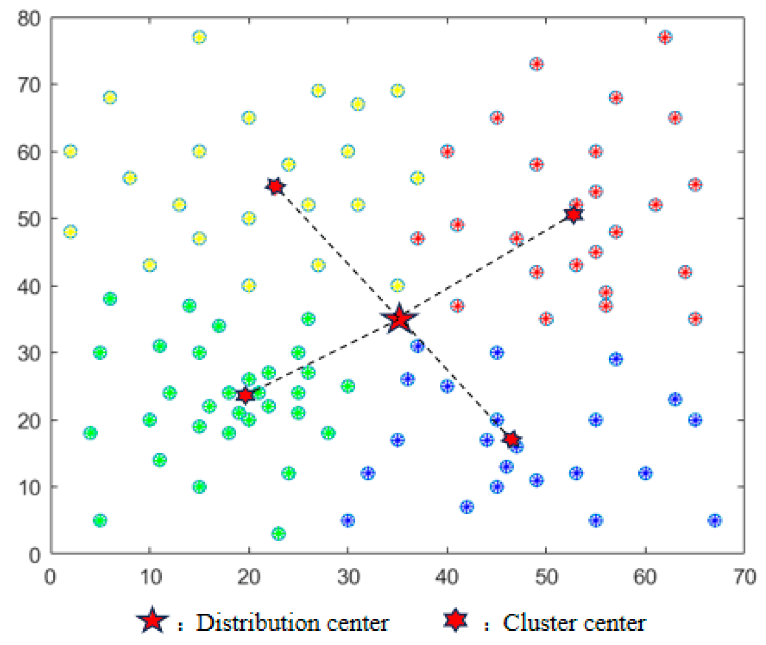
4.1. Simulation of Clustering Problem

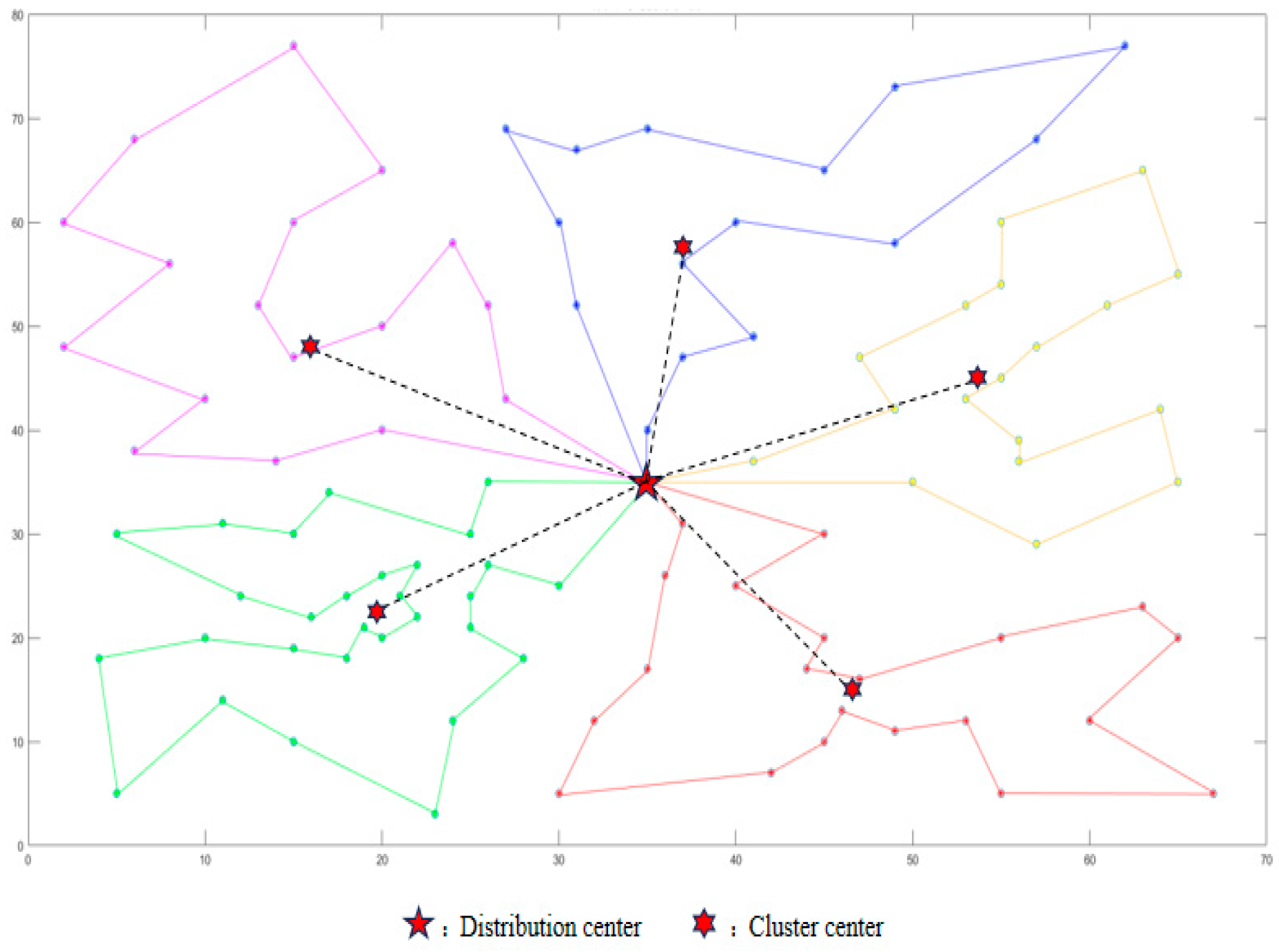
4.1.1. Clustering Results Analysis

The algorithmic parameters are configured as follows: clustering is performed sequentially based on the UAV fleet size, with a power exponent of 3, a convergence tolerance of 1 × 10⁻⁶, a cooling rate of 0.8, an initial temperature of 100, a terminal temperature of 1, a population size of 10, maximum generations of 600, a crossover rate of 0.7, and a mutation rate of 0.05.

For scenarios involving three, four, and five UAVs performing simultaneous deliveries, three, four, and five clustering centers are set, respectively. The 100 customer points are clustered accordingly. The clustering results for the three cases are shown in Figure 6, Figure 7 and Figure 8. The optimal customer point function value $J_b$ is obtained for each clustering. The respective values are 6.7913 × 10³, 3.5142 × 10³, and 2.2198 × 10³, where smaller values indicate better clustering performance, and the results demonstrate stability.

4.1.2. Comparison of Clustering Algorithms

Also, for the above case, the FCM algorithm is used to perform a clustering simulation on 100 target points, and the cases with three, four, and five clustering centers are calculated five times, respectively. The results are shown in

Table 3. Clustering results.

Number of Clustering Centers	Frequency	Jb Value of FCM (×103)	FCM Mean Jb Value (×103)	Jb Value of SA-GA-FCM (×103)
3	1	6.9033	6.8410	6.7913
	2	6.8316
	3	6.8142
	4	6.8119
	5	6.8442
4	1	3.8362	3.6810	3.5142
	2	3.6927
	3	3.5145
	4	3.7761
	5	3.5852
5	1	2.2211	2.2312	2.2198
	2	2.2374
	3	2.2450
	4	2.2221
	5	2.2306

.

It can be seen from the table that the clustering results of the FCM algorithm are different every time, while the SA-GA-FCM algorithm is more stable, and the Jb value is the same every time. The average Jb value obtained by performing the FCM algorithm five times is compared with that of the SA-GA-FCM algorithm. In the above three cases, the Jb value of the SA-GA-FCM algorithm is reduced by 0.0497 × 10³, 0.1668 × 10³, and 0.0114 × 10³, respectively, compared with that of FCM algorithm. Therefore, the clustering effect of the SA-GA-FCM algorithm is better.

4.2. Simulation of Path Problem

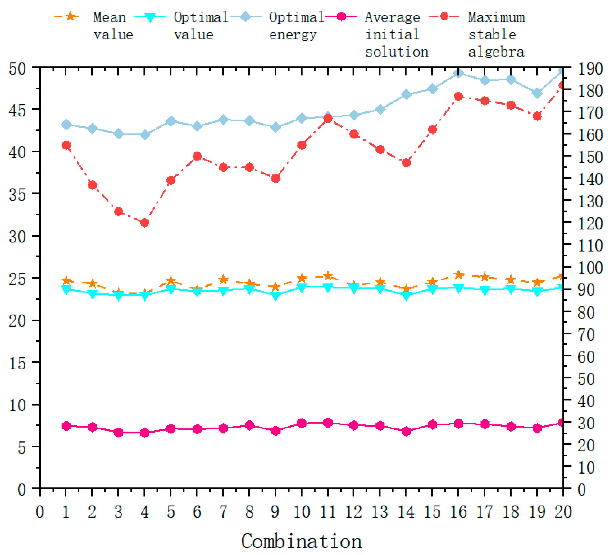
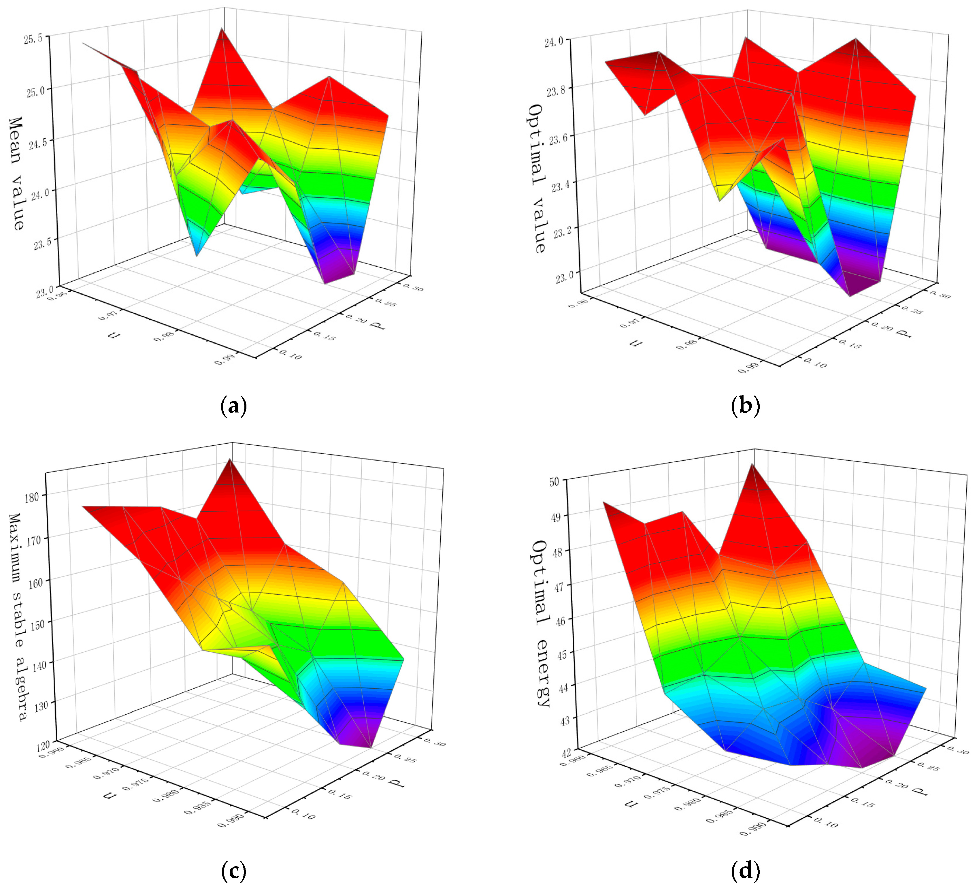
4.2.1. Parameter Sensitivity Analysis

The delivery situation of UAV 1 in the first clustering case is selected as the reference. As the setting of the dynamic step parameter in the IHNN in this paper will have an impact on the optimization process, in order to explore the optimization results of the IHNN algorithm, the values of u and P in a dynamic step are analyzed, and A is set to 1.5, C is 2, D is 1, and the maximum number of iterations is 600, which is 0.02. On the basis of 10 continuous runs, the influence of the different combinations of u and P in a dynamic step on the optimization process is analyzed.

As can be seen from

Table 4. Parameter sensitivity experimental results.

Combination	u	p	Mean Value	Average Initial Solution	Optimal Value	Maximum Stable Algebra	Optimal Energy
1	0.99	0.10	24.693	28.374	23.738	155	43.246
2	0.99	0.15	24.358	27.891	23.196	137	42.765
3	0.99	0.20	23.245	25.456	22.984	125	42.135
4	0.99	0.25	23.197	25.298	22.984	120	42.012
5	0.99	0.30	24.693	27.123	23.746	139	43.657
6	0.98	0.10	23.629	26.987	23.432	150	43.042
7	0.98	0.15	24.817	27.345	23.575	145	43.802
8	0.98	0.20	24.319	28.648	23.786	145	43.680
9	0.98	0.25	23.975	26.235	22.984	140	42.913
10	0.98	0.30	24.988	29.583	23.957	155	43.978
11	0.97	0.10	25.244	29.875	23.981	167	44.146
12	0.97	0.15	24.143	28.634	23.836	160	44.346
13	0.97	0.20	24.536	28.458	23.810	153	45.024
14	0.97	0.25	23.718	25.985	22.984	147	46.791
15	0.97	0.30	24.543	28.996	23.765	162	47.468
16	0.96	0.10	25.421	29.432	23.901	177	49.340
17	0.96	0.15	25.129	29.198	23.636	175	48.458
18	0.96	0.20	24.798	28.134	23.789	173	48.596
19	0.96	0.25	24.469	27.457	23.467	168	46.967
20	0.96	0.30	25.325	29.928	23.894	182	49.685

, there are certain differences in the mean value, average initial solution, optimal value, maximum stable algebra, and optimal energy value obtained by the simulation under different parameter combinations, indicating that the IHNN algorithm has differences in the solution effect for different parameters u and P, but the overall difference is not big. The results obtained after running the algorithm under different combinations of the two parameters 10 times are shown in Figure 9 and Figure 10 below.

Combined with the above chart, it is not difficult to find that the IHNN algorithm has differences in the solution effect for different parameters u and p. When the value of u is close to 1 at 0.99, the overall solution effect is better, while when p is 0.25, the mean value, average initial solution, optimal value, maximum stable algebra, and optimal energy value obtained by the simulation all reach optimal levels. Therefore, the parameters are set to u = 0.99 and p = 0.25, and the subsequent path optimization problem is solved to obtain the optimal scheme.

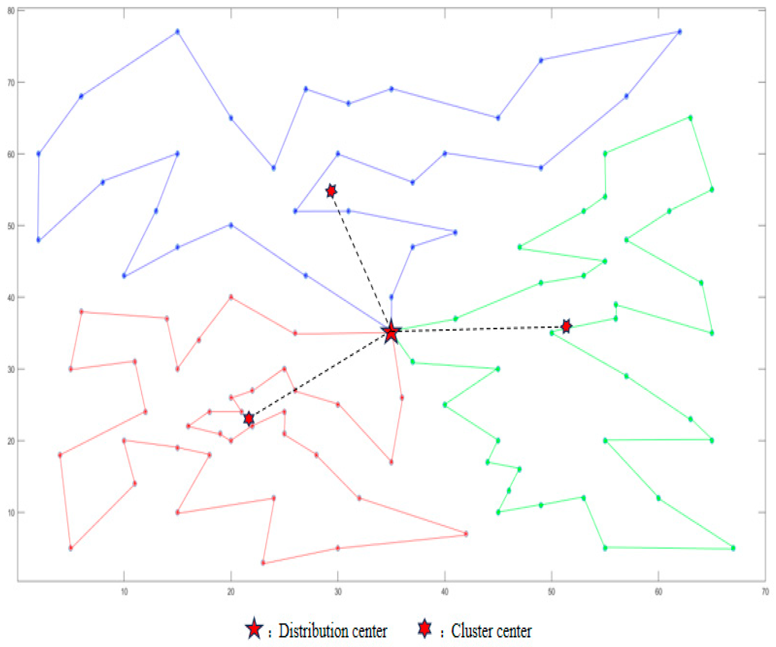
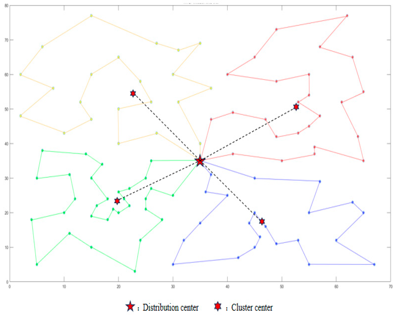
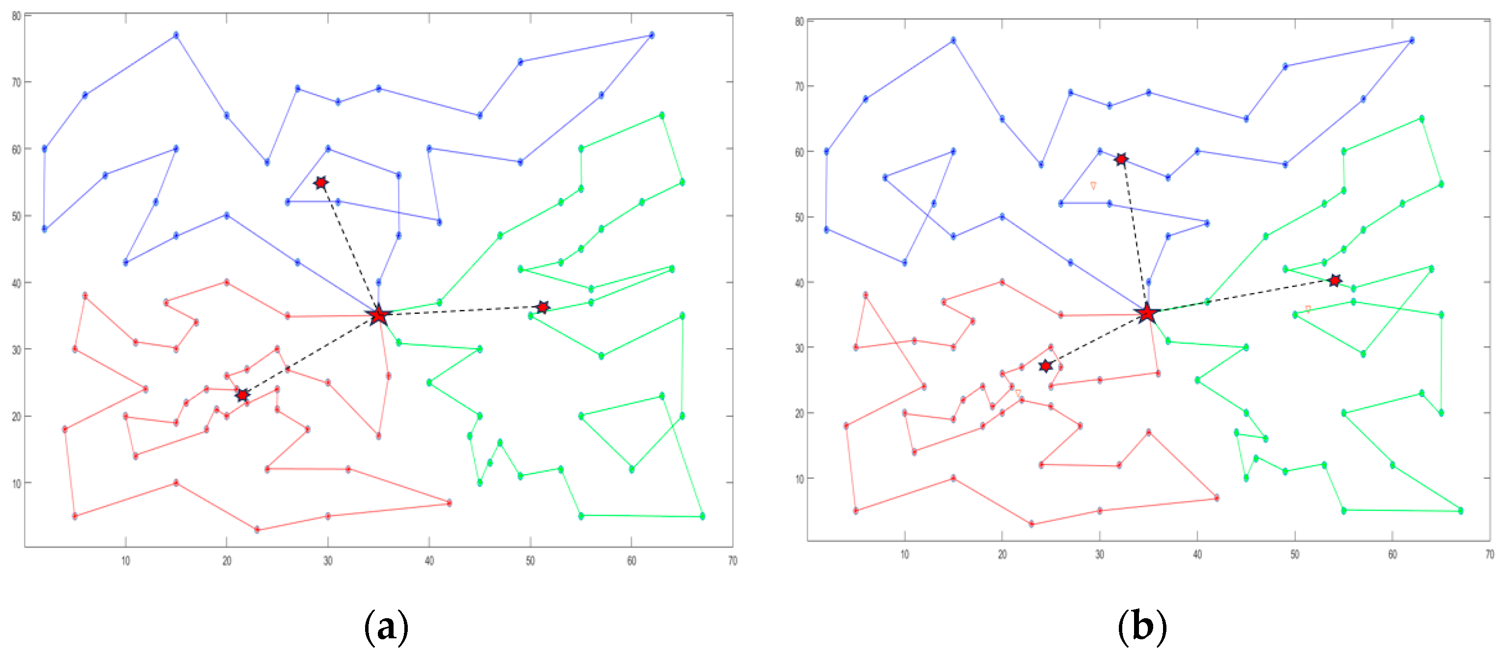
4.2.2. Path Simulation Analysis

Based on the clustering results of the three cases, simulations are carried out, respectively. Combined with the optimal path optimization scheme, as shown in Figure 11, Figure 12 and Figure 13, each UAV sequentially services all assigned customer nodes before returning to the distribution center, ensuring complete coverage without service omissions or route conflicts throughout the mission. This shows that the optimization has a certain effect and the task assignment is reasonable. The specific path optimization results are shown in

Table 5. Path optimization results.

Situation	UAV	Cluster Center	Number of Customers	Path Length (km)	Total Length of Air Route (km)	Delivery Time (min)	Algorithm Runtime (×10−3 s)
One	1	(51.35, 35.86)	34	22.984	70.133	27.58	54.899
	2	(21.62, 23.07)	37	22.553		27.06	58.827
	3	(29.35, 54.88)	29	24.596		29.52	47.280
Two	1	(22.67, 54.54)	22	19.165	71.383	23.00	46.039
	2	(46.38, 17.11)	22	16.063		19.28	45.277
	3	(19.59, 23.56)	31	17.957		21.55	49.346
	4	(52.60, 50.66)	25	18.198		21.84	47.165
Three	1	(46.60, 15.53)	21	16.096	75.118	19.32	40.447
	2	(19.74, 22.48)	29	16.819		20.18	47.198
	3	(15.98, 47.93)	17	13.941		16.73	35.578
	4	(53.83, 44.98)	18	13.223		15.87	35.771
	5	(37.10, 57.36)	15	15.039		18.05	32.342

.

4.2.3. Comparison of Optimization Algorithms

We select the scenario with three UAVs from the first clustering case as the reference. In addition to the IHNN algorithm designed in this paper, the standard genetic algorithm and the ant colony optimization algorithm are also used for solving the problem. The parameters for the standard genetic algorithm are consistent with those set in Section 3.1. The parameter settings for the ant colony optimization algorithm are as follows: the number of ants is 31, the pheromone importance factor is 1, the heuristic function importance factor is 5, the pheromone evaporation rate is 0.1, the constant coefficient is 1, and the maximum number of iterations is 600. Each of the three algorithms is run independently 15 times. The path diagrams generated by the genetic algorithm and ant colony algorithm are shown in Figure 12. The specific data for the three algorithms are shown in

Table 6. Algorithm comparison results.

UAV	Algorithm	Number of Iterations	Path Length	Delivery Time (min)	Algorithm Running Time (×10−3 s)
1	IHNN	120	22.984	27.58	54.899
	ACA	270	23.503	28.20	95.818
	GA	210	23.834	28.60	84.544
2	IHNN	110	22.553	27.06	58.827
	ACA	250	23.249	27.90	98.567
	GA	230	23.468	28.16	88.402
3	IHNN	150	24.596	29.52	47.280
	ACA	280	24.775	29.73	88.256
	GA	260	24.816	29.78	81.952

, and a result comparison diagram is shown in Figure 14.

It can be clearly seen from the Figure 14 that in the path diagrams generated by the ant colony algorithm and genetic algorithm, the paths cross to varying degrees, and the effect is weaker than that of the IHNN algorithm designed in this paper.

It can be seen from the Figure 15 that the path length and delivery time of the IHNN algorithm are reduced to varying degrees compared with the genetic algorithm and ant colony algorithm. In terms of the number of iterations, the number of iterations for the three paths of the IHNN is 120, 110 and 150, respectively, and the number of iterations is also reduced to a certain extent compared with the other two algorithms. In terms of the algorithm running time, the three solution times of the IHNN are 0.054899, 0.058827, and 0.047280, respectively, and the running time is faster than the other two algorithms. Therefore, the hybrid optimization algorithm developed using the Hopfield neural network has better convergence, higher solution efficiency, and better results.

The energy function in a neural network is a mathematical function used to describe the state of the neurons. It helps the network find the optimal weights and bias parameters during the training process, thereby improving the model’s performance and accuracy. The following figure shows the energy function graph generated during the delivery path optimization process for three UAVs in Scenario 1. A smaller energy function value indicates that the neuron state is more stable, whereas a higher value suggests instability or noise interference. As shown in the Figure 16, the energy function for all three paths stabilizes at its minimum value within 200 generations, with the minimum value being below 100. These experimental results substantiate the efficacy of the proposed algorithmic framework.

5. Conclusions

The authors researched the route optimization problem of multi-UAV collaborative delivery, and the principal findings of this study can be summarized as follows:

(1)

A clustering algorithm is used to cluster the large-scale customer points, and the UAVs are delivered to the areas that need service. A stable clustering value is obtained each time, and the clustering effect is good.

(2)

In terms of path optimization, the IHNN algorithm designed in this paper has an improved computation efficiency, convergence, and results, and the shortest path and iteration times are reduced to different degrees compared with the genetic algorithm and ant colony algorithm.

Combining the above two improved algorithms can enable multiple UAVs to complete collaborative distribution tasks more efficiently. In the follow-up, we will further consider the three-dimensional paths of UAVs in the distribution process; the dynamic conditions; the UAV path combined with economic benefits; and the mode of vehicle–machine collaborative distribution with UAVs, taking trucks into account.

References

1. Liu, Z.; Li, X. Optimization model of cold chain logistics delivery path based on genetic algorithm. Int. J. Ind. Eng. Theory Appl. Pract. 2024, 31, 152. [Google Scholar]
2. Chen, C.; Luo, Z.; Du, S. Optimization of electric vehicle-UAV collaborative distribution path under partial charging strategy. J. Chang. Univ. Sci. Technol. 2025, 1–11. [Google Scholar] [CrossRef]
3. Wang, J.Q.; Gao, X.G.; Shi, J.G.; Li, B. Unmanned Aerial Vehicle’s Path Planning for Scout. Fire Control Command. Control 2008, 33, 16–18. [Google Scholar]
4. Fu, Z.T.; Hu, Z.H.; Fei, H.P. Hazardous container yard patrol optimization research with UAVS. J. Railw. Sci. Eng. 2017, 14, 2467–2471. [Google Scholar] [CrossRef]
5. Liu, W.B.; Wang, Y.D. Path planning of Multi-UAV cooperative search for multiple targets. Electron. Opt. Control 2019, 26, 35–38, 73. [Google Scholar]
6. Cao, Z.K. UAV-Based Land Surveying Route Planning and Scheduling. J. Geomat. 2021, 46, 64–67. [Google Scholar]
7. Mao, H.T.; Shi, J.M.; Zhou, Y.Z.; Liu, Z. Small UAV routing planning for reconnaissance missions with recharging. J. Command. Control 2022, 8, 206–213. [Google Scholar]
8. Wang, S.; Lv, X.; Li, Y.; Jing, L.; Fang, X.; Peng, G.; Zhou, Y.; Sun, W. A novel hybrid improved dingo algorithm for unmanned aerial vehicle path planning. J. Braz. Soc. Mech. Sci. Eng. 2025, 47, 10. [Google Scholar] [CrossRef]
9. Hu, K.; Mo, Y. A novel unmanned aerial vehicle path planning approach: Sand cat optimization algorithm incorporating learned behaviour. Meas. Sci. Technol. 2024, 35, 046203. [Google Scholar] [CrossRef]
10. Wang, Z.; Sun, G.; Zhou, K.; Zhu, L. A parallel particle swarm optimization and enhanced sparrow search algorithm for unmanned aerial vehicle path planning. Heliyon 2023, 9, e14784. [Google Scholar] [CrossRef]
11. Ait-Saadi, A.; Meraihi, Y.; Soukane, A.; Yahia, S.; Ramdane-Cherif, A.; Gabis, A.B. An enhanced African vulture optimization algorithm for solving the unmanned aerial vehicles path planning problem. Comput. Electr. Eng. 2023, 110, 108802. [Google Scholar] [CrossRef]
12. Van Nguyen, L.; Kwok, N.M.; Ha, Q.P. Fermat-Weber location particle swarm optimization for cooperative path planning of unmanned aerial vehicles. Appl. Soft Comput. 2024, 167, 112269. [Google Scholar] [CrossRef]
13. Hopfield, J.J.; Tank, D.W. Neural computation of decisions in optimization problems. Biol. Cybern. 1985, 52, 141–152. [Google Scholar] [CrossRef]
14. Chen, X.; Ruan, C. An improvement of Hopfield network to solve TSP algorithm. J. Beijing Univ. Posts Telecommun. 1996, 99–102. [Google Scholar]
15. Dang, J.; Jin, F. Research on the application of neural network in solving MTSP. J. China Railw. Soc. 1997, 64–70. [Google Scholar]
16. Wang, C.; Xuan, G. A new method of artificial neural network to solve TSP problem. Comput. Appl. Softw. 2001, 59–65. [Google Scholar] [CrossRef]
17. Yan, C.; Wang, Z. Research on TSP problem based on improved energy function and transient chaotic neural network. J. Syst. Simul. 2006, 1402–1405. [Google Scholar]
18. Jolai, F.; Ghanbari, A. Integrating data transformation techniques with Hopfield neural networks for solving travelling salesman problem. Expert Syst. Appl. 2010, 37, 5331–5335. [Google Scholar] [CrossRef]
19. An, J.L.; Gao, J.; Lei, J.H.; Gao, G.H. An improved algorithm for TSP problem solving with Hopfield neural networks. Adv. Mater. Res. 2011, 143, 538–542. [Google Scholar] [CrossRef]
20. Lin, N.; Liu, H. Dynamic route guidance algorithm based on improved hopfield neural network and genetic algorithm. Int. J. Innov. Comput. Inf. Control 2014, 10, 811–822. [Google Scholar]
21. Guo, Z.; Jin, L.; Zheng, C. Research on improved algorithm of artificial neural network for solving TSP problem. Comput. Simul. 2014, 31, 355–358. [Google Scholar]
22. Tarkov, M.S. Solving the traveling salesman problem using a recurrent neural network. Numer. Anal. Appl. 2015, 8, 275–283. [Google Scholar] [CrossRef]
23. Kai, C. An ad-hoc network routing algorithm based on improved neural network under the influence of COVID-19. J. Intell. Fuzzy Syst. 2020, 39, 8767–8774. [Google Scholar] [CrossRef]
24. Hu, Y.; Duan, Q. Solving the TSP by the AALHNN algorithm. Math. Biosci. Eng. 2022, 19, 3427–3448. [Google Scholar] [CrossRef]
25. Dutta, G. Solving The Travelling Salesmen Problem using HNN and HNN-SA algorithms. arXiv 2022, arXiv:2202.13746. [Google Scholar]
26. Comert, S.E.; Yazgan, H.R.; Turk, G. Hopfield neural network based on clustering algorithms for solving green vehicle routing problem. Int. J. Ind. Eng. Comput. 2022, 13, 573–586. [Google Scholar] [CrossRef]
27. Almuhanna, H.; Alenezi, M.; Abualhasan, M.; Alfadhli, R.; Alajmi, S.; Aldashti, Z.; Salman, M. A Novel Hybrid Solution for Traveling Salesman Problem. In International Conference on Advanced Engineering, Technology and Applications; Springer Nature: Cham, Switzerland, 2024. [Google Scholar]
28. Li, X.; Yang, X.; Ju, X. A novel fractional-order memristive Hopfield neural network for traveling salesman problem and its FPGA implementation. Neural Netw. 2024, 179, 106548. [Google Scholar] [CrossRef]
29. Che, H.; Chen, K.; Wang, Y.; Liu, X. Fuzzy C-means clustering algorithm with deep neighborhood information. J. Huazhong Univ. Sci. Tech. (Nat. Sci. Ed.) 2022, 50, 135–141. [Google Scholar]
30. Bai, L.; Hu, S.; Liu, S. A Fuzzy Clustering Algorithm Based on Simulated Annealing and Genetic Algorithm. Comput. Eng. Appl. 2005, 41, 55–59. [Google Scholar]
31. Xue, J.; Chang, X. Mobile beacon path planning of UWSNs based on Hopfield neural network. Transducer Microsyst. Technol. 2020, 39, 35–42. [Google Scholar]
32. Zhang, X.; Wang, Y.G.; Chen, H.Y.; Hang, W.; Cao, L.; Deng, H.; Yuan, J. Optimization of Fixed-abrasive Tool Development Parameters Based on BP Neural Network and Genetic Algorithm. Surf. Technol. 2022, 51, 358–366. [Google Scholar]
33. Yu, Z.M. Hopfield neural network based on genetic simulated annealing strategy to solve TSP problem. China Water Transp. 2019, 19, 89–91. [Google Scholar]
34. Liu, S.; Chen, S.-J.; Han, Z.-H. Study for Flexible Flow Shop Scheduling Problem with Advanced HNN Algorithm. Control Eng. China 2019, 26, 1667–1674. [Google Scholar]
35. Lv, C.; Xu, J. Multi-compartment vehicle selection and delivery strategy with time windows under multi-objective optimization. Alex. Eng. J. 2023, 85. [Google Scholar] [CrossRef]
Figure 1. Schematic diagram of distribution process.
Wevj 16 00157 g001
Figure 2. Schematic diagram of solution scheme.
Wevj 16 00157 g002
Figure 3. Neuron structure diagram.
Wevj 16 00157 g003
Figure 4. Contrast of asynchronous lengths.
Wevj 16 00157 g004
Figure 5. Flowchart of hybrid algorithm.
Wevj 16 00157 g005
Figure 6. Three clustering centers—clustering renderings.
Wevj 16 00157 g006
Figure 7. Four clustering centers—clustering renderings.
Wevj 16 00157 g007
Figure 8. Five clustering centers—clustering renderings.
Wevj 16 00157 g008
Figure 9. Optimization diagram under different parameter combinations.
Wevj 16 00157 g009
Figure 10. Influence of different parameter combinations on each result. (a) Effects of different parameter combinations on mean value. (b) Influence of different parameter combinations on optimal value. (c) Effect of different parameter combinations on number of iterations. (d) Effects of different parameter combinations on optimal energy.
Wevj 16 00157 g010
Figure 11. Optimal distribution path of three UAVs.
Wevj 16 00157 g011
Figure 12. Optimal distribution path of four UAVs.
Wevj 16 00157 g012
Figure 13. Optimal distribution path of five UAVs.
Wevj 16 00157 g013
Figure 14. Path graphs generated by different algorithms. (a) Paths generated by ant colony algorithm. (b). Path generated by genetic algorithm.
Wevj 16 00157 g014
Figure 15. Comparison of algorithm effects.
Wevj 16 00157 g015
Figure 16. Energy function diagram.
Wevj 16 00157 g016