Intelligent Vehicle Trajectory Tracking Based on Horizontal and Vertical Integrated Control

Abstract

To address the common issues of accuracy and stability in trajectory tracking tasks for autonomous vehicles, this study proposes an innovative composite control strategy that skillfully integrates lateral and longitudinal dynamic control. For lateral control, model predictive control (MPC) theory is introduced to compute the front wheel steering angle that ensures optimal trajectory following. On the longitudinal control level, the vehicle’s acceleration and deceleration logic are finely tuned to ensure precise adherence to the preset speed trajectory. More importantly, by deeply integrating these two control methods, the comprehensive coordination of the vehicle’s lateral and longitudinal movements is achieved. To validate the effectiveness of the proposed control strategy, simulations were conducted using the CarSim and MATLAB/Simulink platforms. The analysis of the simulation results confirms that the proposed method effectively improves speed tracking stability and significantly enhances path tracking accuracy and overall driving stability.

1. Introduction

With the increasing global emphasis on environmental protection, the adoption rate of intelligent vehicles is rapidly escalating [1]. These vehicles not only rely on advanced battery technologies and propulsion systems but also on sophisticated control strategies, particularly precise trajectory tracking control, to ensure optimal performance and safety across diverse driving conditions. In electric and hybrid vehicles, accurate trajectory tracking is essential for optimizing energy management, reducing energy consumption, enhancing driving comfort, and enabling autonomous driving capabilities. Trajectory tracking control is a fundamental component, designed to follow the desired trajectory outlined by the upper-level planning module while maintaining vehicle stability through high-precision tracking. Currently, predominant trajectory tracking control algorithms include the front-wheel feedback control algorithm (Stanley algorithm [2]), the pure pursuit algorithm, proportional–integral–derivative (PID) control [3], the linear quadratic regulator (LQR) tracking controller, and model predictive control (MPC).

The Stanley algorithm uses the distance from the center of the front axis to the nearest reference track point as a basic nonlinear feedback function, which can make the lateral tracking error converge to zero, so as to achieve high-precision track tracking. However, the algorithm requires high smoothness of the expected path. In the case of uneven road curvature, it can lead to excessive vehicle response, which can cause safety hazards and driving discomfort in complex urban environments. Pan Shiju et al. [4] proposed an intelligent vehicle path-following method based on feedback pure tracking, which makes up for the shortcomings of traditional pure tracking control algorithms by dynamically adjusting the forward-looking distance according to vehicle speed and path curvature, and taking lateral deviation as a feedback variable. However, the traditional pure tracking algorithm is based on the Ackerman steering model, and although the control parameters are fewer and the debugging is simple, the tracking error may increase significantly at high speeds, so it is only suitable for trajectory tracking at low speeds. Although the PID control algorithm [5] was developed in the early stage and is relatively mature, it can obtain the control quantity through the calculation of the proportion, integral, and differential, but it lacks the modeling ability of the controlled object. PID parameters need to be re-adjusted when the vehicle state or external conditions change, making it less flexible in complex driving environments and difficult to achieve a wide range of asymptotic stability. As a result, the applicability of PID in high-speed and complex environments is limited. The improved LQR control algorithm proposed by Zhou Weiqi et al. [6] eliminates the lateral steady-state error by adding feedforward control and introduces the concept of vehicle body deviation to optimize the control strategy, thereby reducing the risk of collision with obstacles. The adaptive LQR control algorithm with preview compensation proposed by Zeng Ying et al. [7] combined with the redundant joint control strategy can adjust the weight of the controller in real time, considering the lateral offset, speed, and road curvature of the vehicle, and significantly improve the accuracy and robustness of trajectory tracking. However, the adaptability of the LQR in dealing with nonlinear constraints and complex conditions is limited, especially when the dynamic characteristics of the vehicle or environmental factors change dramatically; the weight adjustment process may lead to a decrease in control accuracy. In addition, the selection of weights relies on extensive debugging, making it difficult to ensure global optimization. In contrast, model predictive control (MPC) [8] can effectively handle constraints such as vehicle dynamics, control input range, and collision avoidance while taking into account multiple objectives such as error minimization, energy minimization, and comfort maximization. For example, the MPC-based trajectory tracking algorithm proposed by Xie Xianyi et al. [9] performs better than the traditional LQR algorithm in terms of lateral error and centroid deflection control accuracy, and it has less fluctuation and overshoot. However, the real-time computing burden of MPC and the high demand for computing resources may limit its effectiveness in some application scenarios with strict real-time requirements. Finally, the adaptive learning MPC method proposed by Zhang et al. [10] is designed to solve the trajectory tracking problem with input constraints, while considering efficiency, safety, and stability. Despite the good performance of the method, the training process of the learning algorithm in practical applications and its adaptability to environmental changes still need to be further studied to ensure high efficiency and stability in dynamic driving scenarios. The intelligent electric vehicle track tracking controller based on MSC-PID proposed by Hu Linzhi [11] provides a good tracking effect in different speed intervals, and the front wheel angle and yaw angle speed change smoothly, ensuring high tracking accuracy and certain robustness. However, the combination of MPC and PID increases the complexity of the controller and can create a potential bottleneck in real time due to computing resources, especially in highly dynamic driving scenarios where the demand for computing power is high and can limit the real-time response speed. The MPC lateral controller and the double-ring PID longitudinal controller based on the road curvature model proposed by Zhou Yipang et al. [12] calculate the optimal front wheel angle through the MPC, and the double-ring PID controller controls the unmanned vehicle to achieve the desired speed according to the speed error and position error. The scheme demonstrates good stability and accuracy in path tracking control and improves the comfort of longitudinal speed control. However, the efficiency and robustness of double-loop PID control in vertical control depend on the accuracy of preset parameters and the ideality of the system, and the adjustment of PID parameters still needs to be further optimized. In addition, the independent design of dual controllers may not be able to effectively deal with nonlinear dynamics caused by horizontal and vertical coupling, which may affect the overall trajectory tracking performance.

Building on the current research achievements, this paper proposes a novel longitudinal and lateral trajectory tracking control strategy based on model predictive control (MPC) and proportional–integral–derivative (PID) control. The lateral tracking control is implemented using the MPC method to determine the optimal control input for the rate of change of the front wheel steering angle. Subsequently, a position–velocity dual PID controller is developed to convert the computed desired acceleration and current vehicle speed into throttle and brake values by referencing calibration tables for the throttle and brakes, thereby realizing longitudinal control of the vehicle. The effectiveness of the proposed control strategy is rigorously validated through co-simulation using Simulink and CarSim.

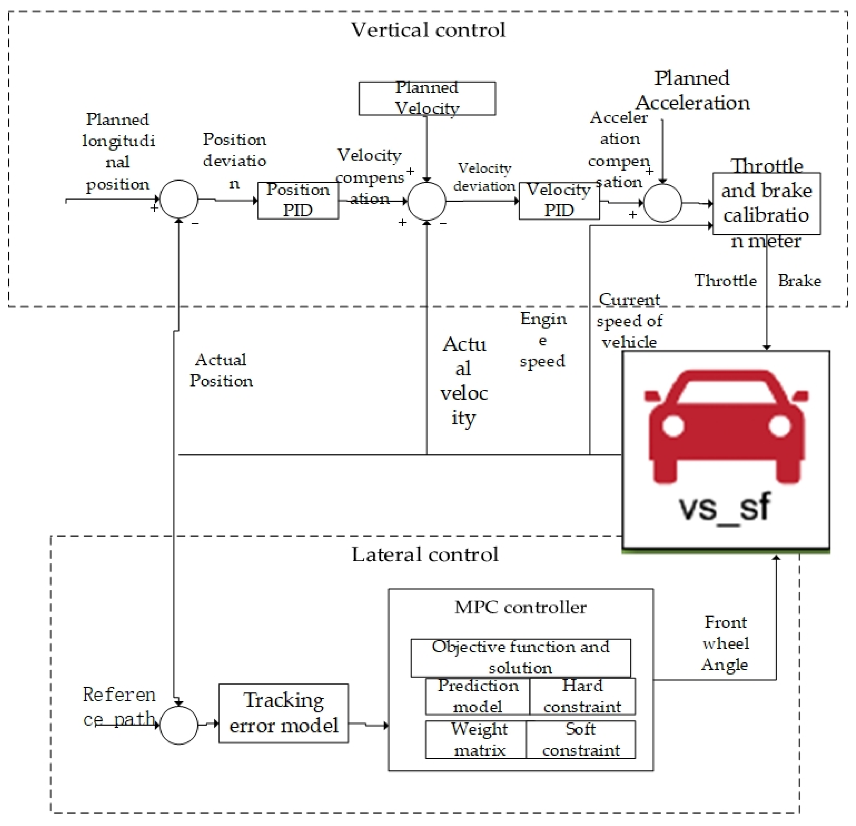
2. Overall Design of Control System

The integrated longitudinal and lateral trajectory tracking control system for intelligent vehicles, illustrated in Figure 1, is structured as follows.

The lateral controller employs model predictive control (MPC) methodologies, utilizing vehicle state and anticipated path data. By means of predictive modeling, rolling optimization, and feedback correction, it applies constraints to the vehicle’s dynamic behavior to ascertain the optimal front wheel steering angle. Conversely, the longitudinal controller determines target vehicle velocities based on the anticipated path and implements effective acceleration and deceleration strategies to ensure the vehicle converges towards the desired speed. The combined longitudinal and lateral control system integrates actual vehicle speed as a pivotal parameter, concurrently providing longitudinal velocity data to both controllers for comprehensive management of vehicle dynamics. This approach excels in sustaining the precise tracking of desired trajectories and velocities while fortifying driving stability.

2.1. Establishment of Vehicle Dynamics Model

This study investigates the dynamic model of an intelligent vehicle conceptualized as a system equation, aiming to direct the vehicle along a designated trajectory while minimizing tracking errors arising from measurement noise. The central challenge addressed in this research is how to effectively reduce these tracking errors through a set of control parameters, all while adhering to constraints pertaining to smoothness, acceleration, and speed, thereby ensuring both the accuracy and stability of trajectory tracking.

This research utilizes a two-degree-of-freedom vehicle dynamics model to examine the path accuracy and ride comfort associated with a trajectory tracking controller for autonomous vehicles. The parameters, including vehicle mass, distances from the center of gravity to both the front and rear axles, vehicle moment of inertia, as well as the lateral stiffness of both front and rear wheels, are established factory variables, as depicted in Figure 2.

The model specifically focuses on the lateral motion of the vehicle and yaw dynamics around the Z axis, operating under the following assumptions [13]:

(1)

Suspension system effects are disregarded, assuming front-wheel steering configuration.

(2)

The vehicle’s movement is constrained to the horizontal plane, omitting vertical dynamics.

(3)

Vehicle speed remains nearly constant throughout the analysis.

(4)

Aerodynamic influences on the vehicle are excluded from consideration.

(5)

Each tire is assumed to possess identical mechanical characteristics, with no additional lateral forces or restoring moments factored in.

(6)

The vehicle maintains constant rotational inertia, and there is no lateral displacement of the center of mass, ensuring minimal lateral load variation.

Based on the two-degree-of-freedom dynamic model of the vehicle shown in Figure 2 for force analysis, the dynamic differential equations for lateral motion and yaw motion of the vehicle can be obtained:

$$\left\{\begin{array}{l}m{a}_y=F_{yf}\cos \delta +F_{yf}-F_{xf}\sin \delta \\ I\dot{\phi }=a{F}_{yf}\cos \delta -b\left(F_{yf}-F_{xf}\sin \delta \right)\end{array}\right.$$

(1)

In the formula, $F_{yf}$ and $F_{yr}$ are the lateral forces of the front and rear wheels of the vehicle ($\mathrm{N}$); $F_{xf}$ and $F_{xr}$ are the longitudinal force of the front and rear wheels of the vehicle ($\mathrm{N}$); $a$ and $b$ are the distance from the vehicle’s center of mass to the front and rear axles ($\mathrm{m}$); $m$ represents the mass of the car ($\mathrm{kg}$); $a_y$ is the lateral acceleration of the vehicle (${\mathrm{m}/\mathrm{s}}^2$); $\dot{\phi }$ is the lateral angular velocity of the vehicle (deg/s); $I$ is the moment of inertia of the vehicle relative to the Z axis ($\mathrm{kg}\ast {\mathrm{m}}^2$); $\delta$ is the front wheel steering angle.

According to the kinematic relationship, the acceleration components $a_x$ and $a_y$ of the vehicle’s center of mass in the x and y axis directions can be derived.

$$\left\{\begin{array}{l}{a}_x={\dot{v}}_x-v_y\dot{\phi }\\ a_y={\dot{v}}_y+v_x\dot{\phi }\end{array}\right.$$

(2)

Generally, $\delta$ is relatively small, so $\cos \delta =1$; $\sin \delta =0$. There is:

$$\left\{\begin{array}{l}m\left({\dot{v}}_y+v_x\dot{\phi }\right)=F_{yf}+F_{yr}\\ I\ddot{\phi }=a{F}_{yf}-b{F}_{yr}\end{array}\right.$$

(3)

In the formula, $\ddot{\phi }$ is the angular acceleration of vehicle yaw. The relationship between the tire side deflection angle and tire side deflection force is shown in Formula (4):

$$\left\{\begin{array}{l}{F}_{yf}=C_{\alpha f}{\alpha }_f\\ F_{yr}=C_{\alpha r}{\alpha }_r\end{array}\right.$$

(4)

In the formula, ${\alpha }_f$ and ${\alpha }_r$ represent the front and rear wheel side deflection angle (rad); $C_{\alpha f}$ and $C_{\alpha r}$ indicate that the side deflection stiffness (N/rad) of the front and rear wheels of the car is negative. According to the right-hand rule, when the side deflection force of the tire is positive, the side deflection angle is negative.

Substituting Equation (4) into Equation (3) yields the following:

$$\left\{\begin{array}{l}m\left({\dot{v}}_y+v_x\dot{\phi }\right)=C_{\alpha f}{\alpha }_f+C_{\alpha r}{\alpha }_r\\ I\ddot{\phi }=a{C}_{\alpha f}{\alpha }_f-b{C}_{\alpha r}{\alpha }_r\end{array}\right.$$

(5)

Under the premise of no sideslip, the side deflection angle of the tire can be derived as follows:

$$\left\{\begin{array}{l}{\alpha }_f={\displaystyle \frac{v_y+a\dot{\phi }}{v_x}}-\delta \\ {\alpha }_r={\displaystyle \frac{v_y-b\dot{\phi }}{v_x}}\end{array}\right.$$

(6)

Substituting Equation (6) into Equation (5) yields and arranges the following:

$$\left\{\begin{array}{l}{\dot{v}}_y={\displaystyle \frac{C_{\alpha f}+C_{\alpha r}}{m{v}_x}}{v}_y+\left({\displaystyle \frac{a{C}_{\alpha f}-b{C}_{\alpha r}}{m{v}_x}}\right)\dot{\phi }+\left(-{\displaystyle \frac{C_{\alpha f}}{m}}\right)\delta \\ \ddot{\phi }={\displaystyle \frac{a{C}_{\alpha f}-b{C}_{\alpha r}}{I{v}_x}}{v}_y+{\displaystyle \frac{a^2{C}_{\alpha f}+b^2{C}_{\alpha r}}{I{v}_x}}\dot{\phi }+\left(-{\displaystyle \frac{a{C}_{\alpha f}}{I}}\right)\delta \end{array}\right.$$

(7)

At this stage, the controlled system can be described by the following state space expression:

$$\left\{\begin{array}{l}\dot{\mathrm{\xi }}=f(\mathrm{\xi },\mathrm{u})\\ \mathrm{\eta }=C\mathrm{\xi }\end{array}\right.$$

(8)

In the formula, the state quantity is $\mathrm{\xi }={\left[\dot{y},\dot{\phi }\right]}^T$ and the control quantity is $u=[{\mathrm{\delta }}_f]$. $\eta$ is the output and $C$ is the identity matrix.

The simplified two-degree-of-freedom vehicle dynamics model, characterized by its intrinsic simplicity and user-friendly application, enables rapid computations; consequently, it is deemed an efficient framework that enhances the responsiveness of control systems.

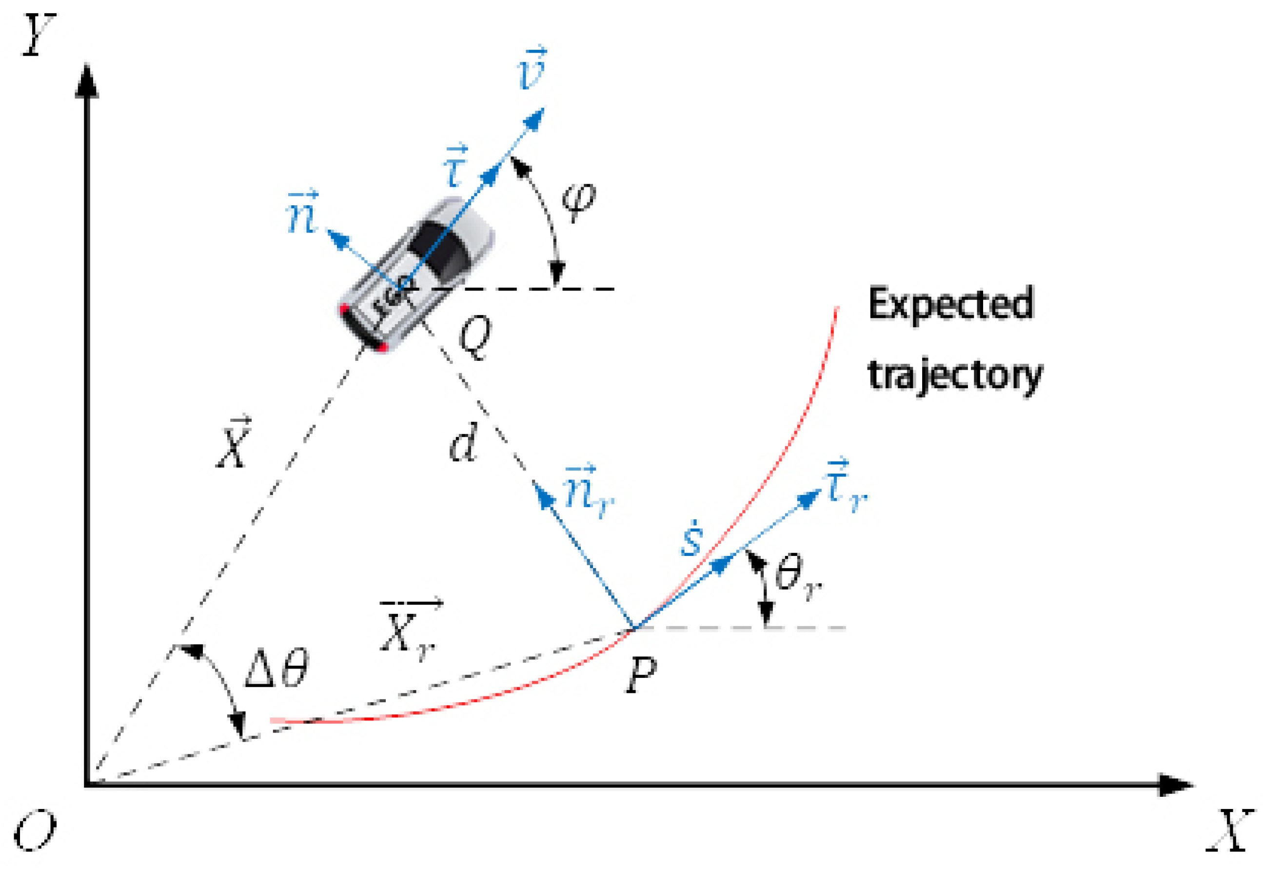
2.2. Establishment of the Tracking Error Model

In the previous section, the vehicle dynamics model has been established. In order to achieve perfect tracking of the path information sent by the planning layer, the tracking error model is commonly used in the motion control of autonomous vehicles [14]. Let $Q=\left(x,y\right)$ be the vehicle position and $P=\left(x_r,y_r\right)$ be the projection point of the vehicle on the desired trajectory. s is the arc length of the curve and the unit tangent vector along the expected trajectory. The unit tangent vector, unit normal vector, and velocity vector are established at points Q and P. Point Q is represented by the position vectors $\overrightarrow{\tau }$, $\overrightarrow{n}$, and $\overrightarrow{v}$, while point P is represented by the position vectors ${\overrightarrow{\tau }}_r$, ${\overrightarrow{n}}_r$, and $\overrightarrow{s}$. The position vectors $\overrightarrow{X}$ and ${\overrightarrow{X}}_r$ correspond to points Q and P, respectively. Figure 3 illustrates this path tracking error model.

As depicted in the figure, $d$ represents the lateral error between the vehicle and the expected trajectory. The heading error, denoted as $e_{\phi }=\phi -{\theta }_r$, is defined as the difference between the heading angle of the vehicle and the angle formed by the tangent line and the X axis of the vehicle at point P on the projected trajectory. The unit tangent vector and unit normal vector of the vehicle centroid are represented by $\overrightarrow{\tau }$ and $\overrightarrow{n}$, respectively. By considering these geometric relationships, we can derive the following:

$$d=(\overrightarrow{X}-{\overrightarrow{X}}_r)\cdot {\overrightarrow{n}}_r$$

(9)

Differentiating both sides of Equation (9) yields the following:

$$\dot{d}=\left(\overrightarrow{\dot{X}}-{\overrightarrow{\dot{X}}}_r\right)\cdot {\overrightarrow{n}}_r+\left(\overrightarrow{X}-{\overrightarrow{X}}_r\right)\cdot {\overrightarrow{\dot{n}}}_r$$

(10)

The derivative of the vector representing the actual vehicle position and its projected position can be expressed as follows:

$$\left\{\begin{array}{l}\overrightarrow{\dot{X}}=\left|\overrightarrow{v}\right|\overrightarrow{\tau }\\ {\overrightarrow{\dot{X}}}_r=\dot{s}{\overrightarrow{\tau }}_r\end{array}\right.$$

(11)

The model-based assumption posits that it is minimal, denoted by $e_d=d$. By employing the Frenet formulas, Equation (11) is substituted into (10) to derive the following.

$$\left\{\begin{array}{l}{\dot{e}}_d=v_x\sin e_{\phi }+v_y\cos e_{\phi }\\ \dot{s}={\displaystyle \frac{1}{1-k_r{e}_d}}\left[v_x\cos e_{\phi }-v_y\sin e_{\phi }\right]\end{array}\right.$$

(12)

After being arranged, we possess the following:

$$\left\{\begin{array}{l}{v}_y={\dot{e}}_d-v_x{e}_{\phi }\\ {\dot{v}}_y={\ddot{e}}_d-v_x{\dot{e}}_{\phi }\\ \dot{\phi }={\dot{e}}_{\phi }+{\dot{\theta }}_r\\ \ddot{\phi }={\ddot{e}}_{\phi }({\ddot{\theta }}_{r}minute, inconsequential quantity.)\end{array}\right.$$

(13)

By substituting Equation (13) into the vehicle dynamic model in Equation (7), we derive the following:

$$\left\{\begin{array}{l}{\ddot{e}}_d=\left({\displaystyle \frac{C_{\alpha f}+C_{\alpha r}}{m{v}_x}}\right){\dot{e}}_d+\left(-{\displaystyle \frac{C_{\alpha f}+C_{\alpha r}}{m}}\right)e_{\phi }+\left({\displaystyle \frac{a{C}_{\alpha f}-b{C}_{\alpha r}}{m{v}_x}}\right){\dot{e}}_{\phi }+\left(-{\displaystyle \frac{C_{\alpha f}}{m}}\right)\delta +({\displaystyle \frac{a{C}_{\alpha f}-b{C}_{\alpha r}}{m{v}_x}}-v_x){\dot{\theta }}_r\\ {\ddot{e}}_{\phi }=\left({\displaystyle \frac{a{C}_{\alpha f}-b{C}_{\alpha r}}{I{v}_x}}\right){\dot{e}}_d+\left(-{\displaystyle \frac{a{C}_{\alpha f}-b{C}_{\alpha r}}{I}}\right)e_{\phi }+\left({\displaystyle \frac{a^2{C}_{\alpha f}+b^2{C}_{\alpha r}}{I{v}_x}}\right){\dot{e}}_{\phi }+\left(-{\displaystyle \frac{a{C}_{\alpha f}}{I}}\right)\delta +\left({\displaystyle \frac{a^2{C}_{\alpha f}+b^2{C}_{\alpha r}}{I{v}_x}}\right){\dot{\theta }}_r\end{array}\right.$$

(14)

The state space representation of Equation (14) with the error control system’s state variable ${\left[e_d,{\dot{e}}_d,e_{\phi },{\dot{e}}_{\phi }\right]}^T$ and the control variable for the front wheel steering angle $\delta$ can be expressed as follows:

$${\dot{e}}_{rr}=A{e}_{rr}+Bu+C{\dot{\theta }}_r$$

(15)

In the formula, $A=\left[\begin{array}{cccc}0& 1& 0& 0\\ 0& {\displaystyle \frac{C_{\alpha f}+C_{\alpha r}}{m{v}_x}}& -{\displaystyle \frac{C_{\alpha f}+C_{\alpha r}}{m}}& {\displaystyle \frac{a{C}_{\alpha f}-b{C}_{\alpha r}}{m{v}_x}}\\ 0& 0& 0& 1\\ 0& {\displaystyle \frac{a{C}_{\alpha f}-b{C}_{\alpha r}}{I{v}_x}}& -{\displaystyle \frac{a{C}_{\alpha f}-b{C}_{\alpha r}}{I}}& {\displaystyle \frac{a^2{C}_{\alpha f}+b^2{C}_{\alpha r}}{I{v}_x}}\end{array}\right]$, $B=\left[\begin{array}{c}0\\ -{\displaystyle \frac{C_{\alpha f}}{m}}\\ 0\\ -{\displaystyle \frac{a{C}_{\alpha f}}{I}}\end{array}\right]$, $\mathrm{C}=\left[\begin{array}{c}0\\ {\displaystyle \frac{a{C}_{\alpha f}-b{C}_{\alpha r}}{m{v}_x}}-v_x\\ 0\\ {\displaystyle \frac{a^2{C}_{\alpha f}+b^2{C}_{\alpha r}}{I{v}_x}}\end{array}\right]$, $e_{rr}={\left[e_d,{\dot{e}}_d,e_{\phi },{\dot{e}}_{\phi }\right]}^T$, and $u=\delta$.

3. Design of Cross- and Longitudinal Tracking Controllers

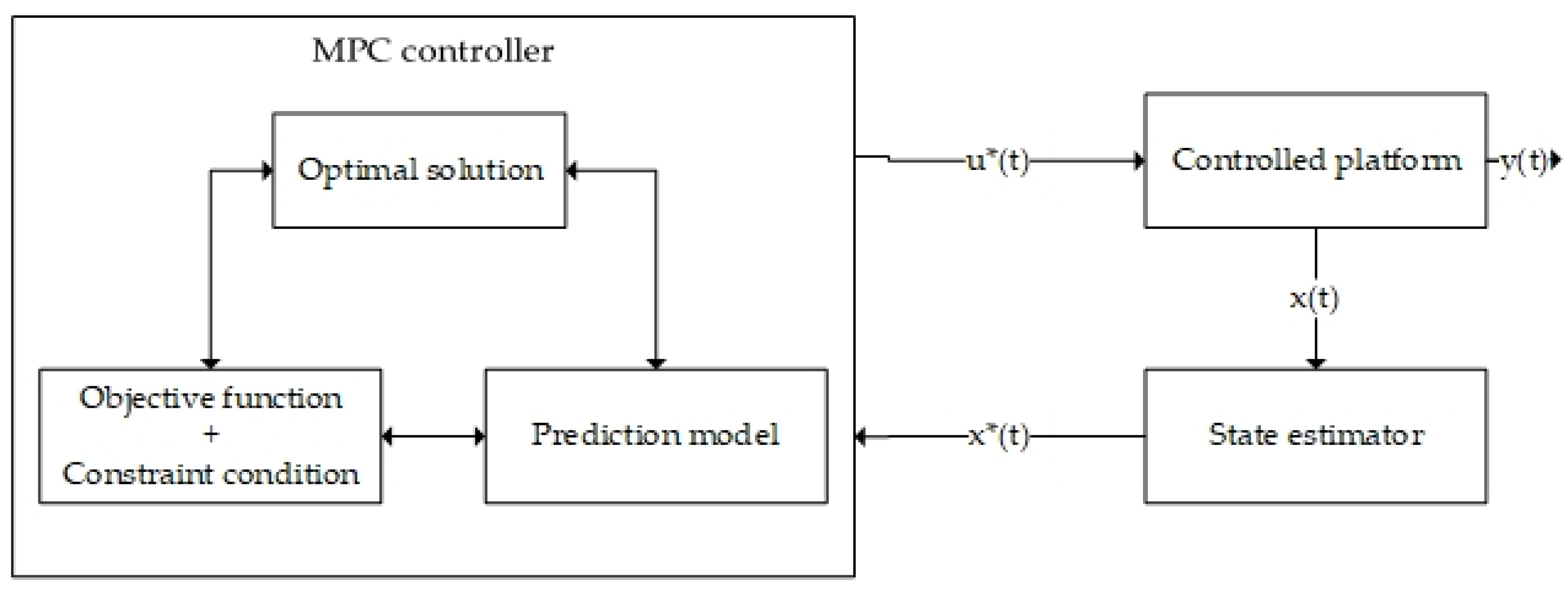
3.1. Design of Lateral Model Predictive Controller

The process depicted in Figure 4 is governed by the control strategy of model predictive control.

In each control cycle, the open-loop control problem within a finite time domain is optimized and continuously iterated for feedback control. The vehicle’s nonlinear dynamic model is linearized, discretized, and augmented with constraints, thereby reformulating it as a quadratic programming problem for resolution.

3.1.1. Linearization and Discretization of Nonlinear Systems

By performing a Taylor expansion of the system equation $\dot{\mathrm{\xi }}=f(\mathrm{\xi },\mathrm{u})$ at points $\mathrm{\xi }={\mathrm{\xi }}_0$, $u=u_0$, and subsequently linearizing the vehicle’s nonlinear dynamics model, we derive a linear time-varying equation.

$$\dot{\mathrm{\xi }}(t)=A_{t,0}\mathrm{\xi }(t)+{\mathrm{B}}_{t,0}u(t)+D_{t,0}$$

(16)

In the formula, $A_{t,0}={\left.{\displaystyle \frac{\partial f}{\partial \mathrm{\xi }}}\right|}_{({\mathrm{\xi }}_0,u_0)}$, $B_{\mathrm{t},0}={\left.{\displaystyle \frac{\partial f}{\partial u}}\right|}_{({\mathrm{\xi }}_0,u_0)}$, and $D_{t,0}=f({\mathrm{\xi }}_0,u_0)-A_{t,0}{\mathrm{\xi }}_0-B_{t,0}{u}_0$.

By employing the forward Euler method, we can derive a discretized equation:

$$\mathrm{\xi }(k+1)=A_{k,t}\mathrm{\xi }(k)+B_{t,0}\mathrm{\xi }(k)+D_{k,t}$$

(17)

In the formula, $A_{k,t}=I+T{A}_{t,0}$, $B_{k,t}=T{B}_{t,0}$, and $D_{k,t}=T{D}_{t,0}$; $I$ is the identity matrix and $T$ is the sampling period.

Let $u(k)=u(k-1)+\Delta u(k)$ and $u(k)$ represent the control increments. Introducing a new state variable $\tilde{\mathrm{\xi }}(k)={[\mathrm{\xi }(k),u(k-1)]}^T$ transforms Equation (17) into a state equation with control increments as inputs, thereby yielding a novel state-space representation.

$$\left\{\begin{array}{l}\tilde{\mathrm{\xi }}(k+1)=\tilde{A}\tilde{\mathrm{\xi }}(k)+\tilde{B}\Delta u(k)+\tilde{D}\\ \eta (k)=\tilde{C}\tilde{\mathrm{\xi }}(k)\end{array}\right.$$

(18)

In the formula, $\tilde{A}=\left[\begin{array}{cc}{A}_{k,t}& B_{k,t}\\ 0& I\end{array}\right]$, $\tilde{B}=\left[\begin{array}{c}{B}_{k,t}\\ I\end{array}\right]$, $\tilde{D}=\left[\begin{array}{c}{D}_{k,t}\\ 0\end{array}\right]$, and $\tilde{C}=\left[\begin{array}{ccccccc}0& 0& 1& 0& 0& 0& 0\\ 0& 0& 0& 0& 1& 0& 0\end{array}\right]$.

In the domain of autonomous driving technology, the primary aim of trajectory tracking control is to ensure that the vehicle’s actual trajectory closely aligns with the predefined ideal path while maintaining vehicular stability. Consequently, when formulating the objective function, two crucial aspects must be considered: firstly, the metric for tracking accuracy, which typically involves quantifying the deviations between the actual and ideal paths; secondly, the stability of the tracking process, which pertains to the system’s ability to withstand disturbances and consistently adhere to the prescribed trajectory [15]. By employing control increments as state variables and integrating relaxation factors, we formulate the objective function as follows:

$$J={\displaystyle {\displaystyle \sum _{i=1}^{N_p}}{‖\eta \left(\mathrm{k}+i|k\right)-{\eta }_{ref}\left(k+i|k\right)‖}_Q^2+{\displaystyle {\displaystyle \sum _{i=1}^{N_c-1}}{‖\Delta u(k+i|k)‖}_R^2}}+\rho {\epsilon }^2$$

(19)

In this expression, $\eta (·\left|k\right.)$ denotes the anticipated control output for a specific time period following time k; ${\eta }_{ref}(·\left|k\right.)$ represents the reference value of $\eta (·\left|k\right.)$; $\Delta u$ signifies the increment of the steering angle of the front wheel; $\rho$ is the weighting coefficient; $\epsilon$ stands for the relaxation factor; $N_p$ pertains to the prediction time domain and $N_c$ relates to the control time domain. Q and R denote, respectively, system output, control increment, and control weight system matrices. The expression is as follows:

$$Q=\left[\begin{array}{cccccc}{Q}_1& 0& \cdots & 0& \cdots & 0\\ 0& Q_2& \cdots & 0& \cdots & 0\\ ⋮& ⋮& \ddots & ⋮& ⋮& ⋮\\ 0& 0& \cdots & Q_i& \cdots & 0\\ ⋮& ⋮& ⋮& ⋮& \ddots & ⋮\\ 0& 0& \cdots & 0& \cdots & Q_{N_p}\end{array}\right]$$

(20)

$$Q_i=\left[\begin{array}{cc}{Q}_{\phi }& 0\\ 0& Q_Y\end{array}\right],i=1,2,3,4,\cdots ,N_p$$

(21)

$$R=\left[\begin{array}{cccccc}{R}_0& 0& \cdots & 0& \cdots & 0\\ 0& R_1& \cdots & 0& \cdots & 0\\ ⋮& ⋮& \ddots & ⋮& ⋮& ⋮\\ 0& 0& \cdots & R_i& \cdots & 0\\ ⋮& ⋮& ⋮& ⋮& \ddots & ⋮\\ 0& 0& \cdots & 0& \cdots & R_{N_c-1}\end{array}\right]$$

(22)

$$R_i=[R_{\delta }],i=0,1,\cdots ,N_c-1$$

(23)

In the objective function, it is necessary to compute the future time-point outputs of the control system. The expression for the system’s future output at various time points is as follows:

$$Y(k)={\psi }_k\xi (k)+{\Theta }_k\Delta U(k)+{\Gamma }_k\Phi$$

(24)

In the formula, $Y(k)=\left[\begin{array}{c}\eta (k+1\left|k\right.)\\ \eta (k+2\left|k\right.)\\ ⋮\\ \eta (k+N_p\left|k\right.)\end{array}\right]$, ${\psi }_k=\left[\begin{array}{c}\tilde{C}\tilde{A}\\ \tilde{C}{\tilde{A}}^2\\ ⋮\\ \tilde{C}{\tilde{A}}^{N_p}\end{array}\right]$, ${\Gamma }_k=\left[\begin{array}{cccc}\tilde{C}& 0& \cdots & 0\\ \tilde{C}\tilde{A}& \tilde{C}& \cdots & 0\\ ⋮& ⋮& \ddots & ⋮\\ \tilde{C}{\tilde{A}}^{N_p-1}& \tilde{C}{\tilde{A}}^{N_p-2}& \cdots & \tilde{C}\end{array}\right]$, $\Phi =\left[\begin{array}{c}{\tilde{D}}_1\\ {\tilde{D}}_2\\ ⋮\\ {\tilde{D}}_{N_p}\end{array}\right]$, ${\Theta }_k=\left[\begin{array}{cccc}\tilde{C}\tilde{B}& 0& 0& 0\\ \tilde{C}\tilde{A}\tilde{B}& \tilde{C}\tilde{B}& 0& 0\\ ⋮& ⋮& \ddots & ⋮\\ \tilde{C}{\tilde{A}}^{N_p-1}\tilde{B}& \tilde{C}{\tilde{A}}^{N_p-2}\tilde{B}& \cdots & \tilde{C}{\tilde{A}}^{N_p-N_c-1}\tilde{B}\end{array}\right]$, and $\Delta U(k)=\left[\begin{array}{c}\Delta u(k\left|k\right.)\\ \Delta u(k+1\left|k\right.)\\ ⋮\\ \Delta u(k+N_c\left|k\right.)\end{array}\right]$.

3.1.2. Reformulate It as a Quadratic Programming Problem for Resolution

In the MATLAB environment, integrate the prediction model and objective function to formulate a trajectory tracking problem using quadratic programming, and define the constraint conditions. Subsequently, utilize the built-in optimization solver quadprog to effectively determine a solution [16].

$$\begin{gathered} \min J={\displaystyle \frac{1}{2}}{\mathrm{x}}^{T}Hx+f^{T}x={\displaystyle \frac{1}{2}}\times 2·{\left[\begin{array}{c}\Delta U\\ \epsilon \end{array}\right]}^T\left[\begin{array}{cc}{\Theta }_k^{T}Q{\Theta }_k+R& 0\\ 0& \rho \end{array}\right]\left[\begin{array}{c}\Delta U\\ \epsilon \end{array}\right]+\left[\begin{array}{cc}2E^{T}Q{\Theta }_k& 0\end{array}\right]\left[\begin{array}{c}\Delta U\\ \epsilon \end{array}\right] \\ s.t.\left\{\begin{array}{c}{U}_{\min }\le U\le U_{\max }\\ \Delta U_{\min }\le \Delta U\le \Delta U_{\max }\\ Y_{\min }\le Y\le Y_{\max }\end{array}\right. \end{gathered}$$

(25)

In the formula, $x$ denotes the vector of return values; $H$ represents the real symmetric quadratic objective matrix; $f$ signifies the linear objective vector; $\mathrm{E}={\psi }_k\xi (k)+{\Gamma }_k\Phi -Y_{ref}(k)$, and $Y_{ref}(k)$ is the reference value for $Y(k)$. Equation (25) should be solved to derive the control input increment sequence $\Delta U_k^{*}={\left[\Delta u_k^{*},\Delta u_{k+1}^{*},\cdots ,\Delta u_{k+N_c-1}^{*}\right]}^T$, followed by taking its first element and adding it to the current control input for application in the controlled system, denoted as $u(k+1)=u(k)+\Delta u_k^{*}$.

When developing a model predictive controller, it is essential to apply constraints to the output, control, and control increment variables. The output variable should be aligned with the vehicle’s reference trajectory, while constraints should be placed on the control and control increment variables specifically, the steering angle of the front wheels, and the steering angle increment [17].

$$\left\{\begin{array}{l}-{15}^{º}\le {\delta }_{\mathrm{f}}\le {15}^{º}\\ -{0.8}^{º}\le \Delta {\delta }_{\mathrm{f}}\le {0.8}^{º}\end{array}\right.$$

(26)

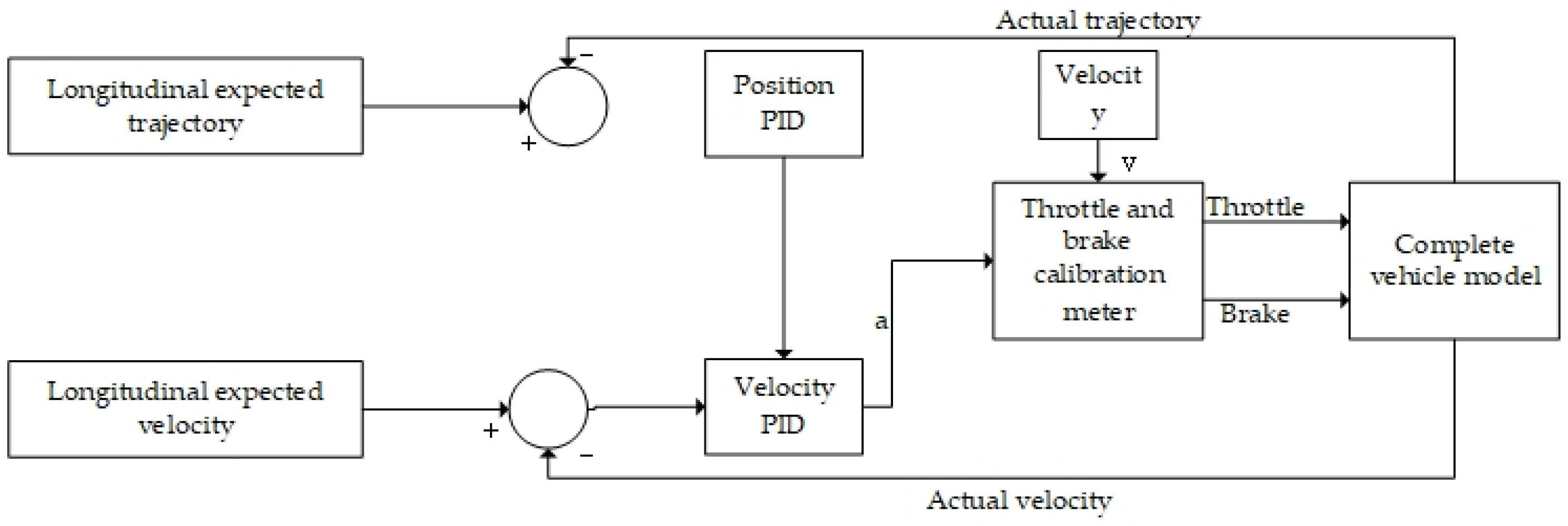
3.2. Design of Vertical Controller

The longitudinal control of autonomous vehicles is primarily achieved by modulating the brakes, accelerator, etc., to regulate the vehicle speed. In this study, a position–speed dual PID controller is employed for implementing longitudinal control. The input of the PID controller is derived from both the planning module’s planning state and the actual state of the CarSim vehicle model. The inverse model encompasses the inverse powertrain system model and the inverse braking system model. The control signal produced by the PID controller is transformed into throttle opening or brake master cylinder pressure by the inverse model and then transmitted to update the vehicle state in the CarSim vehicle model.

The PID, an acronym for proportional–integral–derivative controller, is responsible for adjusting the system’s output by linearly combining the proportional, integral, and derivative control components based on the current error (deviation), the integral of the error, and the rate of change of the error. This adjustment aims to enhance system stability and response speed. The expression is as follows:

$$u(t)=K_{P}e(t)+K_I{\displaystyle {\int }_0^{t}e(t)dt+K_D}{\displaystyle \frac{de(t)}{dt}}$$

(27)

In the formula, $K_P$ represents the proportional coefficient; $K_I$ denotes the integral coefficient; $K_D$ signifies the derivative coefficient; and $e\left(t\right)$ indicates the deviation between the actual system value at time t and the reference value.

Based on the geometric relationship and Equation (12) in the path tracking error model and longitudinal control design, we can derive the longitudinal position deviation $e_s$ and trajectory tracking speed $\dot{s}$. Subsequently, the speed deviation is calculated as follows:

$$\left\{\begin{array}{l}{e}_s=(\overrightarrow{X}-{\overrightarrow{X}}_r)\cdot {\overrightarrow{\tau }}_r\\ e_v=v_r-\dot{s}\end{array}\right.$$

(28)

In the formula, $e_v$ denotes the speed deviation, while $v_r$ signifies the anticipated speed of the trajectory.

Following the aforementioned discussion, this study presents a position–velocity dual PID controller aimed at regulating velocity deviation $e_v$ and position deviation $e_s$, thereby enabling the precise longitudinal tracking of planned position and velocity for the vehicle. The overall longitudinal control block diagram is depicted in Figure 5.

By utilizing the longitudinal position PID controller and longitudinal velocity PID controller to achieve the desired longitudinal acceleration, integrating the current vehicle speed with the desired longitudinal acceleration, and referencing pre-established throttle and brake calibration tables, precise directives for direct vehicle control can be derived. In the simulation experiment section of this study, Simulink and Carsim were combined to construct throttle and brake calibration tables for autonomous vehicles. Initially, throttle control is employed to elevate the vehicle’s longitudinal speed and acceleration while recording corresponding speeds and accelerations at specific throttle values. Subsequently, brake control is applied to decrease the vehicle’s longitudinal speed and acceleration while recording corresponding speeds and accelerations at particular brake values. Ultimately, a comprehensive table detailing throttle and brake values in relation to different speeds and accelerations is obtained for reference during control operations. The input parameters of this calibration table encompass both current vehicle speed as well as desired longitudinal acceleration. Meanwhile, its output consists of either a throttle or brake command that is transmitted to the vehicle model in order to facilitate either acceleration or deceleration.

3.3. Analysis of Stability of Cross and Longitudinal Control Systems

In order to assess the stability of the longitudinal and lateral control systems, model predictive control (MPC) is employed for lateral regulation, while a dual PID strategy is implemented for longitudinal control. The function of the lateral MPC controller: By optimizing the objective function J, MPC ensures stable lateral management, allowing the vehicle to follow its designated path. The function of the longitudinal PID controller is to modify both speed and acceleration in the longitudinal axis, ensuring that stability is preserved without any steady-state error in this dimension. Given that this paper primarily addresses the stability and trajectory tracking accuracy in autonomous driving, the lateral model predictive control (MPC) system assumes greater significance. Consequently, it is essential to initially examine the stability of the lateral system prior to integrating it with the longitudinal control system for a comprehensive analysis of the stability of the coupled system.

3.3.1. Stability Analysis of Lateral MPC Control System

Conduct a Lyapunov stability analysis of the objective function expressed in Formula (19) and derive an appropriate Lyapunov function utilizing the first two terms of this objective function $V\left(x_k\right)$:

$$V\left(x_k\right)={\displaystyle \sum _{i=1}^{N_p}}\parallel \eta (k+i\mid k)-{\eta }_{ref}(k+i\mid k){\parallel }_Q^2$$

(29)

We proceed to demonstrate the non-negativity of this function, where $\parallel \cdot {\parallel }_Q^2$ denotes the weighted quadratic norm. This corresponds to Equation (30):

$$\parallel \eta (k+i\mid k)-{\eta }_{ref}(k+i\mid k){\parallel }_Q^2={(\eta (k+i\mid k)-{\eta }_{ref}(k+i\mid k))}^{T}Q(\eta (k+i\mid k)-{\eta }_{ref}(k+i\mid k))$$

(30)

Given that $Q$ is a positive definite matrix, it follows that $\parallel \eta (k+i\mid k)-{\eta }_{ref}(k+i\mid k){\parallel }_Q^2\ge 0$ holds for all $i$, thereby leading to $V(x_k)\ge 0$.

Moreover, $V\left(x_k\right)=0$ holds if and only if $\eta (k+i\mid k)={\eta }_{ref}(k+i\mid k)$ is satisfied for all $i$. This implies that the system state attains the equilibrium point, specifically $x=0$, at which the Lyapunov function equals $V\left(x_k\right)=0$. Consequently, the non-negativity condition is fulfilled.

The proof of the negative rate of change of the Lyapunov function is presented as follows:

Let us define the error term as $e_i(k)=\eta (k+i\mid k)-{\eta }_{ref}(k+i\mid k)$, and at this stage, $V\left(x_k\right)$ can be expressed as $V\left(x_k\right)={\displaystyle \sum _{i=1}^{N_p}}\parallel e_i(k){\parallel }_Q^2$. We consider the change in $V\left(x_k\right)$ from time $k$ to $k+1$, denoted as $\mathsf{\Delta }V=V(x_{k+1})-V(x_k)={\displaystyle \sum _{i=1}^{N_p}}\left(\parallel e_i(k+1){\parallel }_Q^2-\parallel e_i(k){\parallel }_Q^2\right)$. We assume that the system incorporates an error-decreasing negative feedback mechanism during each update step, such that the change in error satisfies $e_i(k+1)=e_i(k)-\alpha e_i(k)$, where $\alpha >0$ represents the rate of error reduction. By substituting this error update relationship, we obtain $\parallel e_i(k+1){\parallel }_Q^2=\parallel (1-\alpha )e_i(k){\parallel }_Q^2={(1-\alpha )}^2\parallel e_i(k){\parallel }_Q^2$. Consequently, the variation in the Lyapunov function is $\mathsf{\Delta }V=V(x_{k+1})-V(x_k)={\displaystyle \sum _{i=1}^{N_p}}\left({(1-\alpha )}^2-1\right)\parallel e_i(k){\parallel }_Q^2$. Given ${(1-\alpha )}^2-1<0$ (due to $\alpha >0$), we derive $\mathsf{\Delta }V\le -\beta {\displaystyle \sum _{i=1}^{N_p}}\parallel e_i(k){\parallel }_Q^2$, where $\beta =1-{(1-\alpha )}^2>0$ is a constant. Since ${\displaystyle \sum _{i=1}^{N_p}}\parallel e_i(k){\parallel }_Q^2$ is proportional to $\parallel x_k{\parallel }^2$, it can be represented as $V(x_{k+1})-V(x_k)\le -\gamma \parallel x_k{\parallel }^2$ with respect to $\gamma >0$. This indicates that the rate of change of $V\left(x_k\right)$ is negative; when $x\ne 0$ occurs, $V\left(x_k\right)$ will gradually decrease, leading to convergence towards equilibrium point $x=0$ for the system. Therefore, $V\left(x_k\right)$ fulfills the conditions for Lyapunov stability.

Furthermore, the control increment term $\Delta u(k+i|k)$ in the objective function constrains the magnitude of changes in control input, thereby ensuring a smooth and non-oscillatory response. This mitigates the risk of abrupt system responses and enhances its robustness.

Through the construction and analysis of the Lyapunov function, it can be demonstrated that under suitable conditions, this objective function guarantees the asymptotic stability of the system. Consequently, this implies that the state deviation of the control system will converge to zero, enabling smooth tracking of the reference trajectory.

3.3.2. Stability Analysis of Longitudinal PID Control System

A quadratic Lyapunov function $V(e(t))$ is constructed based on Equation (27):

$$V(e(t))={\displaystyle \frac{1}{2}}e{(t)}^2$$

(31)

The differentiation of Equation (31) results in the following:

$$\dot{V}(e(t))=e(t)\dot{e}(t)$$

(32)

According to the PID control law, $\dot{e}(t)$ can be expressed as a combination of proportional, integral, and derivative components. To ensure stability, it is essential to select appropriate values for the control parameters $k_p$, $k_i$, and $k_d$ within the system so that $\dot{V}(e(t))<0$ holds for all $e(t)\ne 0$. This indicates that the system error will progressively diminish over time and ultimately achieve stability.

3.3.3. Stability Analysis of Horizontal and Vertical Integrated Control System

The integration of lateral model predictive control (MPC) with longitudinal proportional–integral–derivative (PID) control creates a holistic control framework. To evaluate the overall stability of this system, it is essential to take into account the interaction effects between these two elements:

A combined Lyapunov function, $V_{total}=V(x_k)+V(e(t))$, can be formulated that includes both lateral and longitudinal control error components. The time derivative of this Lyapunov function must meet the condition ${\dot{V}}_{total}\le -\alpha \parallel x_t{\parallel }^2-\beta \parallel e(t){\parallel }^2$, with $\alpha >0$ and $\beta >0$ denoting the convergence rates within the system. This suggests that both lateral and longitudinal control systems will gradually approach their target trajectories, resulting in an error nearing zero, thus confirming asymptotic stability for the entire configuration.

In summary, the closed-loop arrangement described here represents a stable and dependable solution.

4. Tracking Simulation and Result Analysis

4.1. Vehicle Parameters and Road Model

To assess the efficacy of the longitudinal and lateral integrated control intelligent car tracking system proposed in this study, a combined simulation utilizing CarSim and MATLAB/Simulink was conducted. In this paper, the C-Class model provided in Carsim is selected for simulation verification. The relevant parameters of the vehicle model are presented in

Table 1. Vehicle-related parameters.

Related Parameters	Numerical Value
Vehicle mass/kg	1270
Distance from center of mass to front axis/m	1.015
Distance from center of mass to rear axis/m	1.895
Moment of inertia of the vehicle/(kg·m2)	1536.7
Front wheel side stiffness/(N/rad)	−67,656
Rear wheel side stiffness/(N/rad)	−65,000

.

In the assessment of vehicle stability, the double-lane change test is frequently employed [18]. Based on this, a corresponding driving path was devised, and the specific simulation environment settings included optimal road conditions, an initial vehicle speed of 0 m/s, and tracking from the origin of coordinates. The equation representing the condition for the double-lane change test is as follows:

$$\left\{\begin{array}{l}Y={\displaystyle \frac{d_{y1}}{2}}(1+\tanh z_1)-{\displaystyle \frac{d_{y2}}{2}}(1+\tanh z_2)\\ z_1={\displaystyle \frac{2.4}{25}}(X-27.19)-1.2\\ z_2={\displaystyle \frac{2.4}{21.95}}(X-56.46)-1.2\\ d_{y1}=4,d_{y2}=5.75\end{array}\right.$$

(33)

Table 2. Horizontal and vertical controller parameters.

Related Parameters	Numerical Value
Position Proportion $k_p$	2
Position Integration $k_i$	0.5
Position Differentiation $k_d$	0.1
Speed Proportion $k_p$	1.8
Speed Integration $k_i$	0.8
Speed Differentiation $k_d$	0.1
Prediction time domain $N_p$	20
Control time domain $N_c$	20
Sampling period $T/s$	0.05
$Q$	$\left[\begin{array}{cccc}30& 0& 0& 0\\ 0& 1& 0& 0\\ 0& 0& 6& 0\\ 0& 0& 0& 1\end{array}\right]$
$R$	10

shows the relevant parameters of the horizontal and vertical controllers.

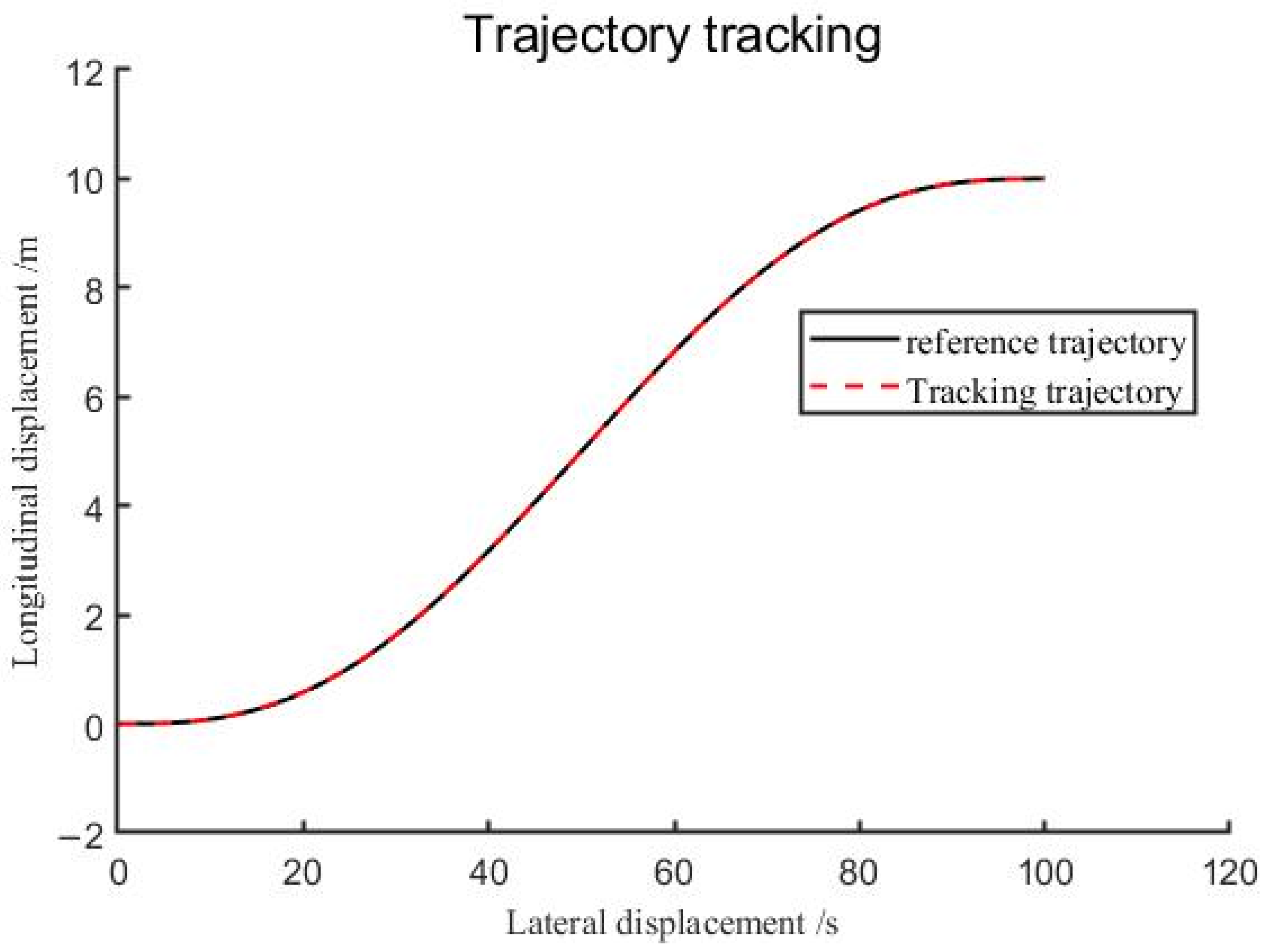
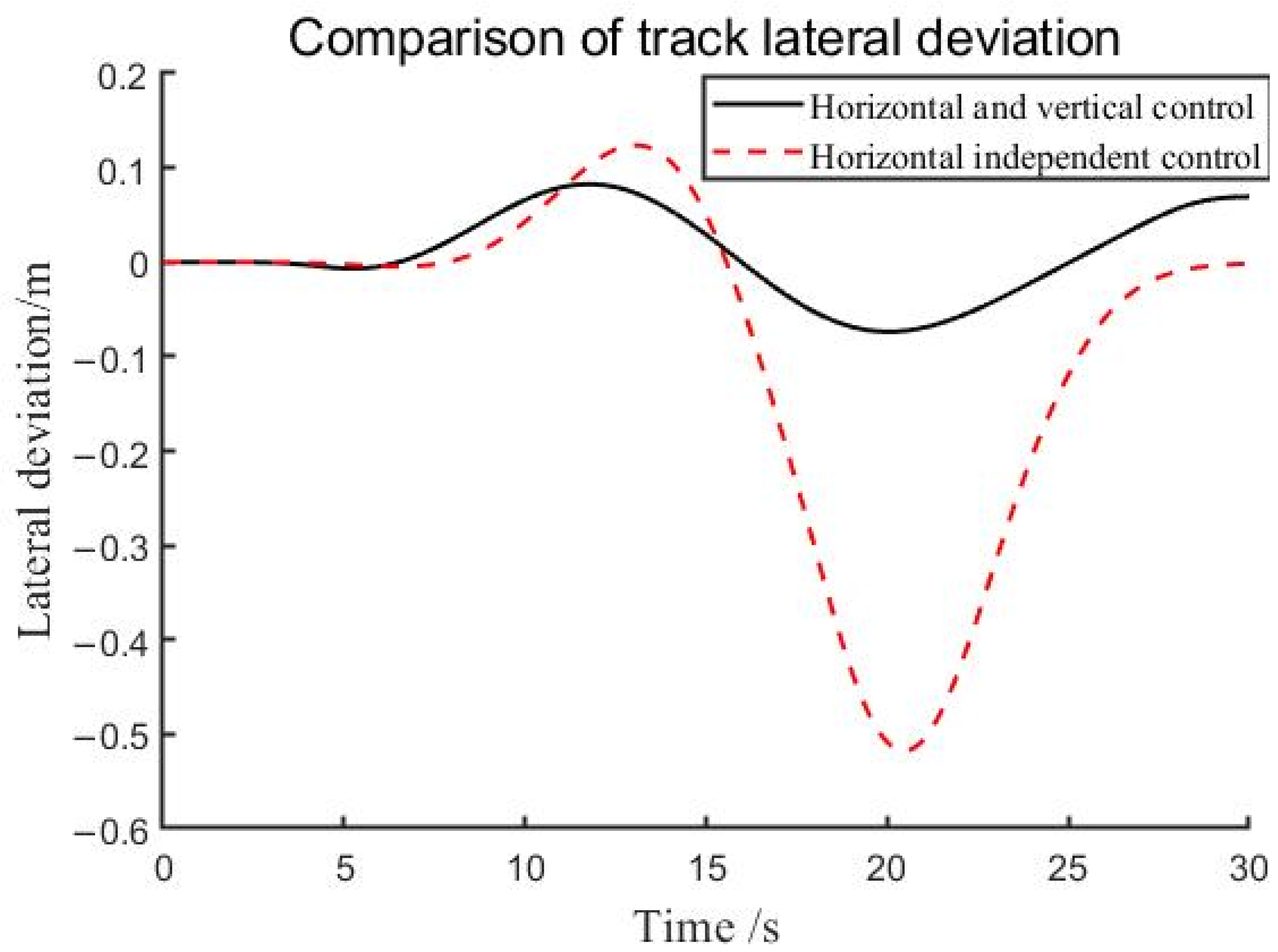
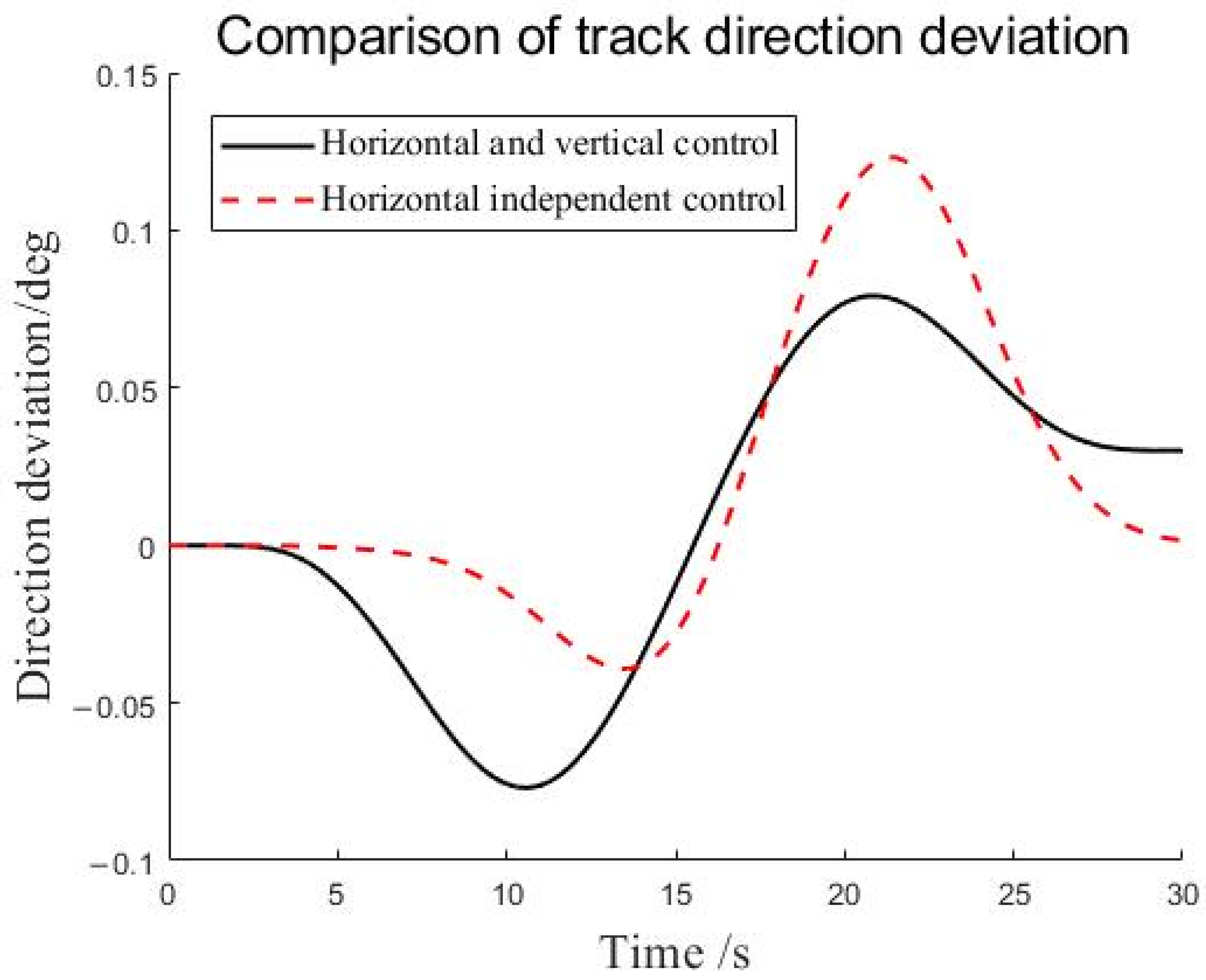
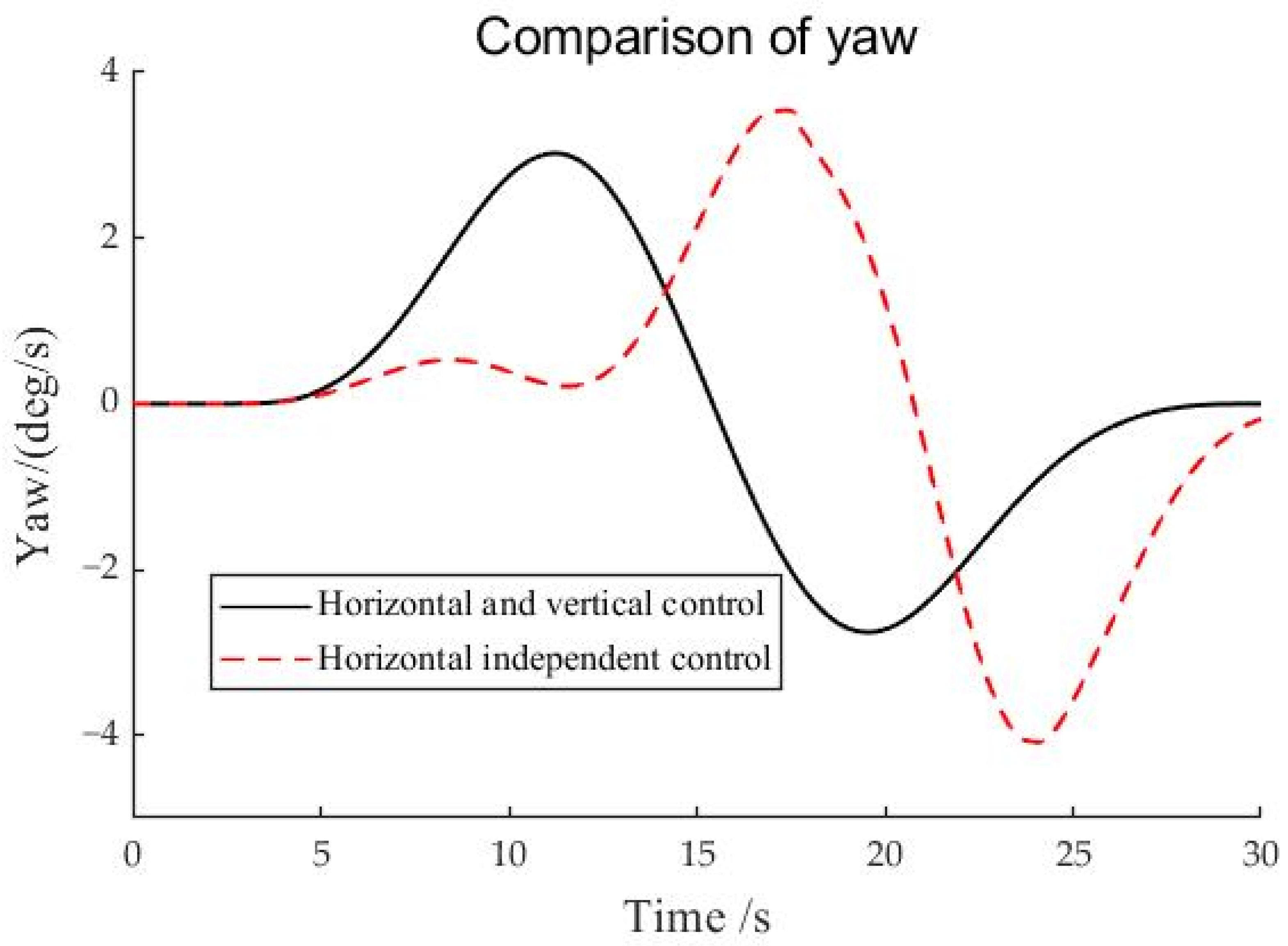
4.2. Simulation Analysis

The horizontal and vertical control systems illustrated in the figure represent the outcomes of operating the system under horizontal model predictive control (MPC) and vertical dual proportional–integral–derivative (PID) control, whereas the horizontal independent control signifies that the system operates solely under horizontal MPC.

Figure 6 is the reference track tracking effect diagram of the horizontal and vertical control system. Initially, the trajectory tracking accuracy was assessed, as illustrated in Figure 7. For the longitudinal and lateral integrated control, the lateral deviation tracking error remained within the range of −0.07–0.07 m, whereas the lateral deviation for independent lateral control was denoted as −0.52–0.12 m. The findings indicate that integrated control significantly mitigates deviations, enabling the vehicle to more closely align with the ideal path and enhancing lateral tracking precision. As depicted in Figure 8, the direction deviation range for longitudinal and lateral integrated control was−0.07–0.07°, outperforming that of independent lateral control at −0.03–0.12°. The reduction in direction deviation signifies that the vehicle is more accurately oriented towards its target path, suggesting superior performance of integrated control regarding path direction precision. These data demonstrate that integrated control facilitates precise path tracking, thereby enhancing both driving safety and passenger comfort within autonomous driving systems. Subsequently, an analysis of vehicle stability was conducted. As shown in Figure 9 during double lane change testing, the yaw rate under longitudinal and lateral integrated control measured −2.8–3.0°/s—lower than −4.1–3.5°/s observed with independent lateral control. This suggests that longitudinal and lateral integrated control produces reduced lateral oscillation during operation, contributing to improved driving stability. Lastly, speed tracking accuracy was evaluated. As indicated in Figure 10, actual vehicle speed under longitudinal and lateral integrated control closely followed target speed levels—enhancing overall stability, the efficiency of travel time management, and safety measures. Experimental data reveal that longitudinal and lateral integrated controls excel over independent methods concerning both tracking accuracy and vehicular stability. The primary advantage of this approach lies in its capacity to synchronize dynamic adjustments of both vehicle speed and directional orientation—better accommodating complex driving scenarios while bolstering safety standards and reliability for autonomous vehicles.

5. Conclusions

To ensure the stable and accurate tracking of desired trajectories by intelligent vehicles, this study leverages previous research findings to propose a comprehensive longitudinal and lateral control method. This method is integrated with the longitudinal vehicle speed and applied in a dual-lane weaving scenario simulation. The key research findings are as follows: Longitudinal tracking control is achieved using the MPC method to optimize the front wheel steering rate. Subsequently, a position–speed dual PID controller is developed to convert the desired longitudinal acceleration and current vehicle speed into throttle/brake values through a lookup table of throttle/brake calibration, thereby achieving effective longitudinal control. Finally, the study combines the longitudinal MPC controller with the longitudinal acceleration/braking controller based on the longitudinal vehicle speed to form an integrated longitudinal and lateral controller. A combined simulation model integrating CarSim and MATLAB/Simulink is utilized to test this comprehensive system in a dual-lane weaving scenario, demonstrating its effectiveness in reducing both lateral and longitudinal positioning errors while maintaining stable changes in key driving parameters. These results validate that the proposed control strategy not only ensures precise longitudinal speed tracking but also enhances trajectory accuracy and vehicle stability.

References

1. Zhao, B.; Wang, H.; Li, Q.; Li, J.; Zhao, Y. PID trajectory tracking control of autonomous ground vehicle based on genetic algorithm. In Proceedings of the 2019 Chinese Control And Decision Conference (CCDC), Nanchang, China, 3–5 June 2019; pp. 3677–3682. [Google Scholar]
2. Zhou, W. Adaptive preview based control system for unmanned vehicle path tracking. Int. J. Veh. Struct. Syst. 2021, 13, 398–404. [Google Scholar] [CrossRef]
3. Marino, R.; Scalzi, S.; Netto, M. Nseted PID steering control for lane keeping in autonomous vehicles. Control. Eng. Pract. 2011, 19, 1459–1467. [Google Scholar] [CrossRef]
4. Pan, S.; Li, J.; Li, H.; Lou, J.; Xu, Y. Path Following Method of Intelligent Vehicles Based on Feedback Pure Tracking Method. Automot. Eng. 2019, 41, 1021–1027. [Google Scholar]
5. Li, S. Overview of Algorithm Research on Trajectory Tracking and Control for Intelligent Vehicles. Automot. Dig. 2023, 9, 19–27. [Google Scholar]
6. Zhou, W.; Zhao, Y.; Liu, Q.; Chen, L. Lateral control strategy of vehicle path tracking based on improved LQR. J. Huazhong Univ. Sci. Technol. (Nat. Sci. Ed.) 2024, 52, 135–141. [Google Scholar]
7. Zeng, Y.; Tang, X.; Lu, X. Redundant control of Automatic driving trajectory Tracking for Complex Road Scenarios. Automot. Pract. Technol. 2024, 49, 11–17+48. [Google Scholar]
8. Vu, T.M.; Moezzi, R.; Cyrus, J.; Hlava, J. Model predictive control for autonomous driving vehicles. Electronics 2021, 10, 2593. [Google Scholar] [CrossRef]
9. Xie, X.; Jin, L.; Du, J. MPC-based trajectory tracking control for autonomous vehicles. J. Mach. Des. 2024, 41, 20–26. [Google Scholar]
10. Zhang, K.; Sun, Q.; Shi, Y. Trajectory tracking control of autonomous ground vehicles using adaptive learning MPC. IEEE Trans. Neural Netw. Learn. Syst. 2021, 32, 5554–5564. [Google Scholar] [CrossRef] [PubMed]
11. Hu, L. Intelligent electric Vehicle trajectory Tracking Control based on MPC-PID. Intell. Comput. Appl. 2019, 14, 155–164. [Google Scholar] [CrossRef]
12. Zhou, Y.; Yang, W. Path Tracking Control of Unmanned Vehicles Based on MPC and PID. Agric. Equip. Veh. Eng. 2019, 61, 78–81+116. [Google Scholar]
13. Chung, S. Research on Tracking Control Method of Autonomous Vehicle Based on Model Predictive Control; South China University of Technology: Guangzhou, China, 2020. [Google Scholar]
14. Zhang, B.; Zhou, B.; Xia, Q. Research on trajectory tracking Control Algorithm of unmanned mining transport Vehicle. J. Automot. Eng. 2024, 14, 168–180. [Google Scholar]
15. Chen, T.; Xu, X.; Cai, Y.; Chen, L.; Sun, X. Coordinated Control of front wheel Angle and yaw stability of unmanned vehicle based on State estimation. J. Beijing Inst. Technol. 2021, 41, 1050–1057. [Google Scholar]
16. Wu, X.; Wei, C.; Zhai, J. Research on Trajectory Tracking Control Optimization of unmanned vehicle considering yaw Stability. Chin. J. Mech. Eng. 2022, 58, 130–142. [Google Scholar]
17. Gong, J.; Jiang, Y.; Xu, W. Autonomous Vehicle Model Predictive Control; Beijing Institute of Technology Press: Beijing, China, 2014. [Google Scholar]
18. Sun, Y. Research on Trajectory Tracking Control Algorithm of Unmanned Vehicle Based on Model Predictive Control; Beijing Institute of Technology: Beijing, China, 2015. [Google Scholar]
Figure 1. Overall horizontal and vertical integrated control diagram.
Wevj 15 00513 g001
Figure 2. Two-degree-of-freedom dynamic model of vehicle.
Wevj 15 00513 g002
Figure 3. Path tracking error model.
Wevj 15 00513 g003
Figure 4. Model predictive control process.
Wevj 15 00513 g004
Figure 5. Position–velocity dual PID longitudinal trajectory tracking control framework.
Wevj 15 00513 g005
Figure 6. Reference track diagram.
Wevj 15 00513 g006
Figure 7. Comparison chart of track lateral deviation.
Wevj 15 00513 g007
Figure 8. Comparison chart of track directional deviation.
Wevj 15 00513 g008
Figure 9. Comparison chart of yaw.
Wevj 15 00513 g009
Figure 10. Vehicle speed tracking.
Wevj 15 00513 g010