Abstract
In this paper, we propose a method for the generation of simulated test scenarios for autonomous driving. Based on the requirements of standard regulatory test scenarios, we can generate virtually simulated scenarios and functional scenario libraries for autonomous driving, which can be used for the simulated verification of different ADAS functions. Firstly, the operational design domain (ODD) of a functional scenario is selected, and the weight values of the ODD elements are calculated. Then, a combination test algorithm based on parameter weights is improved to generate virtually simulated autonomous driving test cases for the ODD elements, which can effectively reduce the number of generated test cases compared with the traditional combination test algorithm. Then, the traffic participant elements in each test case are sampled and clustered so as to obtain hazard-specific scenarios. Then, the values of the subelements under the traffic participant element in each test case are sampled and clustered to obtain hazard-specific scenarios. Finally, the specific scenarios are applied to the automatic emergency braking (AEB) system on the model-in-the-loop (MIL) testbed to verify the effectiveness of this scenario generation method.
1. Introduction
As the level of autonomous driving has increased, the operator of the vehicle has gradually changed from a human to a computer or machine, which requires a large number of tests to prove that driving a car with a machine is safe enough. Automated driving tests are divided into three stages, including virtually simulated tests, closed-field tests, and open-road tests, of which both closed-field tests and open-road tests are real road tests. In the early stage of autonomous driving tests, real road testing faced a large number of problems, such as longer road testing times, higher costs, lower efficiency, the presence of only a single scenario, the inability to guarantee test safety, etc. According to relevant studies, if 100 cars are tested at 40 km per hour, 24 h a day, it will take more than 200 years to test the algorithms of self-driving cars to the same level as human drivers [1]. It is difficult to accept.
Nowadays, with the help of virtual simulation software, virtually simulated testing with reference to the standardized process of testing has become an important part of self-driving car testing. With the development of simulation technology, simulated testing is required to account for more than 90% of the self-driving testing process; closed-field testing accounts for 9%, and open-road testing completes the last 1% of the test volume. These three methods complement each other to accelerate the commercialization of self-driving on the ground.
Several test scenarios can be formed into a test scenario library, and the construction of a simulated test scenario library is one of the focuses of the construction of virtually simulated tests for autonomous driving. The construction of a scenario library includes the generation of scenarios in the scenario library and the evaluation of the scenario library. There are two methods of scenario generation. One is to describe the physical mechanism through expert experience and formulas, parse and reorganize the elements in the scenario, and generate a test scenario through mathematical methods for different test function requirements while expressing the dynamic interaction problem in the scenario as an optimization solution problem and generating the scenario through the optimization solution method. Bagschik et al. [2] studied highway scenarios and proposed an ontology-based scenario generation method. They divided these high-speed scenarios into five levels and used class and logical semantics to realize the modeling and generation of a scenario. Chen et al. [3] studied ramp convergence scenarios and proposed an ontology-based scenario test case generation method. They classified the scenarios into three ontologies of road, weather, and vehicle and realized the generation of scenarios. Kluck et al. [4] combined their ontology with combinatorial testing and proposed an algorithm to map their ontology to combinatorial testing, which was applied to the process of simulation system development. Gao et al. [5] combined the combinatorial testing method with a test matrix to design an automatic scenario generation method and proposed a scenario complexity index to evaluate scenario implementation. Duan et al. [6] proposed a scenario complexity-based combinatorial testing method that uses Bayesian networks to find the balance between scenario complexity and testing cost. This method can find system faults faster and improve testing efficiency. Lee et al. [7] first proposed an adaptive stress test scenario generation method by applying a tree-based reinforcement learning algorithm to solve their problem. They used sampling and forward simulation to progressively build a search tree, modeling the subject as a reinforcement learning training environment that can effectively search for the most likely trajectory leading to an accident by interacting with the environment in real time. This model was subsequently improved upon and introduced to collision avoidance scenario generation for autonomous driving by Koren et al. [8]. These authors described this problem as a Markov decision process, and Monte Carlo tree search (MCTS) and feedforward neural networks were used to find collision scenarios.
The other method of scenario generation is to take collected real natural driving data and accident scenario data and generate scenarios for simulated testing through transformation methods. The U.S. Department of Transportation, in cooperation with the University of Michigan, selected 16 vehicles for a 12 month naturalistic driving data collection effort to study the truck tailgating problem [9]. The US NGSIM dataset, which uses high-definition cameras set up next to highways to collect highway vehicle data, has collected more than 10,000 pieces of data for the study of high-speed tailgating behavior. Accident scene datasets are generally used for the generation of hazard scenes, and Demetriou et al. [10] used the RC-GAN method to establish a deep learning framework based on the driving trajectory data in real accident data to realize the extension of vehicle driving trajectories so as to generate a hazard scene library. Ding et al. [11] proposed a multi-vehicle trajectory generator consisting of a bidirectional encoder and a multi-branch decoder. In their work, multi-vehicle interaction scenes were encoded and sampled to find hazardous scenes. Bolted et al. [12] found the definition of boundaries in hazard scene data and predicted relevant objects at relevant locations in order to identify hazard scenes that have not occurred. Ries et al. [13] introduced a method to efficiently train scene feature extractors using autoencoders, which can identify boundary scenes in a large natural driving dataset. Zhang et al. [14] proposed a Markov chain and Monte Carlo-based method for subset simulation sampling, which solves the problem of difficulty in modeling importance functions in high-dimensional complex scenes.
Based on our analysis of automatic driving simulated test scenario generation methods and evaluation systems, this paper proposes an automatic driving virtually simulated scenario generation method that can be integrated in a generated scenario library covering the realistic standard regulatory test scenarios and small-probability hazardous accident scenarios. Firstly, the simulated test scenarios generated in this paper take functional tests as the demand, introduce operational design domains (ODD), and establish ODD element structures for different functional tests. We then take the values of the third-layer elements in the ODD element structure as the input conditions of the autonomous driving virtual simulation test and at the same time propose a method to assign weights to the ODD element values to obtain the weight values of the ODD element values. Then, an improved test case set generation method is used to improve the existing combination test algorithm by introducing the weight of ODD element values, and the improved ES(a,b) algorithm is obtained to optimize the number of test cases in the test case set generated by the improved algorithm. Then the Monte Carlo method is used to sample the successive elements of the test cases to take values, and the clustering algorithm is used to cluster the sampling results to obtain specific scenarios. Finally, the generated specific scenarios are tested with PreScan and Matlab/Simulink for autonomous driving MIL, which proves the effectiveness of the virtual simulation scenario generation method for autonomous driving based on this paper.
This paper is organized as follows: Section 2 describes the construction of a functional test ODD element structure. Section 3 introduces an improved algorithm for generating test cases for combinatorial testing. Section 4 describes the steps to achieve specific danger scenario generation using Monte Carlo and clustering algorithms. In Section 5, the effectiveness of the method is verified by applying it to an automatic emergency braking (AEB) system. Finally, Section 6 concludes the paper.
2. Methods to Describe Functional Test Scenarios
To generate a virtual simulation test scenario for autonomous driving, it is necessary to determine the input conditions of the scenario, i.e., the values of the elements within the scenario. This section introduces the design operation domain (ODD) for the scenario elements based on functional testing. It also proposes an ODD element assignment method, including subjective assignment method, objective assignment method, subjective-objective integrated assignment method, and absolute weight calculation method in four steps, to get the final weight value of the ODD element taking values.
2.1. Scene Element Design
According to its testing requirements, autonomous driving testing is divided into functional testing, scenario testing, and task testing [15], and this paper selects function as the testing requirement. Functional testing is a test method to verify whether an autonomous vehicle achieves a certain function. The test first determines the function to be tested, and then designs a test scenario according to the function. Compared with scenario testing and task testing, functional testing is more targeted for functional verification.
The Operational Design Domain (ODD) refers to the external environmental conditions and the state of the autonomous driving function of a self-vehicle, as determined during the design phase. The German PEGASUS project identified six layers of ODD-related elements in the scenario, including a road layer, an infrastructure layer, a temporary operational layer, a target object layer, a natural environment layer, and a digital information layer. the Society of Automotive Engineers (SAE) has established a generic ODD terminology and framework consisting of seven dimensions, including weather-related The Association of Standardization of Automation and Measuring Systems (ASAM)’s OpenODD is the openX family of safety standards for the design of operational domains classifies ODDs into three categories: scenarios, environments, and dynamic elements. Scenarios include areas where vehicles travel, intersections or ramps, fixed common road structures, special road structures, and temporary road structures. Environments encompass factors like weather, airborne particulate matter, and lighting conditions. Dynamic elements refer to traffic participants and their vehicles.
In summary, the simulation test scenarios generated in this paper are based on functional tests. For different functional tests, their ODDs are analyzed, and the ODD elements are used as the scene elements in the generated simulation scenarios. The classification of ODDs in the OpenODD and PEGASUS projects are used as the main criteria to design the elements in the ODDs, as shown in Figure 1.
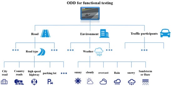
Figure 1.
Autonomous driving function test ODD element structure.
Since the subelements contained under the traffic participant element are mostly the motion states of vehicles, such as: self-vehicle speed, target vehicle speed, target vehicle acceleration, etc., the values of these elements have the characteristics of continuous and unbounded, so the values of the elements need to be discretized. Take the main vehicle speed as an example, the result of discretization processing is shown in Figure 2.
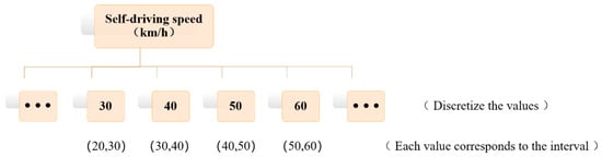
Figure 2.
Discretization of self-driving speed.
2.2. Calculation of Scene Element Taking Weight Value
According to Figure 2, the values of the elements at the bottom of the ODD are used as the values of the scenario elements in the virtual simulation test scenario of autonomous driving. Since the different values of each element at the bottom of the ODD have different weights and importance in the autonomous driving test, it is necessary to assign weights to the elements in the autonomous driving test to quantify their importance.
Weight assignment methods are generally divided into subjective weight assignment method and objective weight assignment method [16]. The subjective weight assignment method is a method in which the evaluator compares the importance of each element based on his or her subjective judgment and calculates the corresponding weight of each element [17]. The advantage of the subjective weighting method is that the relative importance of the elements will not violate people’s common sense; the disadvantage is that the results obtained are more arbitrary. The objective weighting method is a method to determine the weights by calculation based on the objective information of the elements obtained without relying on the subjective attitude of the evaluator [18]. The advantage of the objective weighting method is that the calculation results are based on real data and do not depend on people’s subjective judgment; the disadvantage is that it lacks the complement of subjective consciousness, which will lead to one-sided and single-judgment results.
To combine the advantages and disadvantages of the subjective assignment method and objective assignment method, this paper adopts both the subjective assignment method and objective assignment method to assign the values of ODD elements. The objective assignment method is used to assign the values of the elements in the ODD that can be obtained from the real distribution using published statistics, such as the speed of the vehicle and the weather, while the subjective assignment method is used to assign the values of the remaining elements at the bottom of the ODD.
In this paper, the CRITIC method has been selected to subjectively assign the values of the bottom elements of ODD. This method is an objective assignment method based on data volatility, which determines the objective weight values of the indicators by comparing the intensity and evaluating the conflicting nature between indicators [19].
If there are m rows of the original data set for n values of some third-level element of the ODD, the matrix X is formed:
where denotes the value of the j-th taken value of some third level element of the ODD in the data set of the x-th row, , .
The standard deviation of the j-th value of the element is calculated as:
The variability of the j-th value of the element is calculated as:
Calculate the conflict of the j-th value of the element , denoted by the correlation coefficient :
represents the conflict of the matrix X and is inversely related to the conflict. The larger the , the stronger the correlation between the value of the element and the value of the other elements, the less the conflict, the more information is repeated with the value of the other elements, and therefore the less important information is reflected in the value of the element, and the weight assigned to the value of the element should be reduced [20].
The amount of information for calculating the j-th value of the element taken is:
Finally, the objective relative weight value of the j-th taken value of the ODD element is calculated as:
In this paper, the Analytic Hierarchy Process (AHP) is selected to subjectively assign weights to the values of the lowest element of the ODD. The AHP method is a hierarchical weighting decision analysis method for solving complex multi-objective problems and is widely used in the fields of aerospace and electric power systems [21]. The steps of the AHP are to first take the values of any two elements that belong to the same ODD element and are assigned a quantitative scale that represents the relative influence degree of the function to be measured, and the scale is taken using the 9-quantile scale in the scale method [22].
Assuming that an element of ODD has m taken values, the scale matrix A is obtained according to the proportional scale table as:
The eigenvector corresponding to the largest eigenvalue of the scalar matrix A has been calculated has been calculated, as the subjective relative weight value of these m taken values.
To make the calculated results more reasonable, it is necessary to check the consistency of the feature vectors , which is expressed by the Random consistency ratio (). According to the relevant studies, when , the consistency of the scale matrix A is considered to meet the requirements, and the feature vector calculated by the matrix A can be used as the subjective relative weight of the values taken by the elements of ODD. When , it is necessary to reassign the scaling to the m taken values of the elements and to recalculate the scaling matrix A and the eigenvector .
The stochastic consistency ratio CR is calculated as:
where the Consistency index (CI) is calculated as:
where is the maximum characteristic root of matrix A, which is calculated as:
where is the i-th row of matrix A.
In Equation (8), the value of Average random consistency index (RI) varies with the order m of the scale matrix A, as shown in Table 1.

Table 1.
The Stochastic Consistency Indicator RI takes the value.
The weight values of all the element fetches of the next layer directly subordinated to the elements contained in any layer are calculated by the above-mentioned weight value calculation method. For a multi-level element structure, the absolute weight value for each element in the bottommost level for the values taken by the first level of the target level is obtained by multiplying the weight values taken by each element in each level from the top to the bottom.
In an n-layer system, let there be at most m values taken for an element in any layer, then the absolute weight value for each value taken for the j-th element in the i-th layer is calculated by the formula:
where , , is the set of subscripts of all elements in the j-th element in the i-th layer with the first layer element backtracking path.
3. Improved Combination Testing Methods Based on Parameter Weights
After obtaining the values of functional test ODD elements and their weight values, they are used as the input conditions of the virtual simulation test of autonomous driving for the generation of simulation test scenarios. The traditional scenario generation method mostly adopts the Exhaustive Testing (ET) method in the test case generation method, and the number of generated test cases num is:
where N is the number of influencing factors in the input conditions of the test case, and is the number of values of each influencing factor. When the number of influencing factors and the number of values of each influencing factor is too many, the number of test cases generated by the ET algorithm will be greatly increased, so the Combinatorial Testing (CT) method is often used to generate test cases to reduce the number of test cases generated. In software testing, the failure of a system is generally caused by its own factors and the interaction between factors, so full coverage testing of the combination of factors is required.
In the autonomous driving function test, Zhang et al. [23]. investigated the Lane Departure Warning (LDW) function in autonomous driving, they tested it and found that the faults of the tested functional system were all caused by a single element such as road shape, lane line blurring and missing conditions, and changing conditions of light, and weather conditions. Gao et al. [5] tested the functionality of the body controller system and found that the system produced a total of 21 system defects, of which 16 defects were triggered by specific values of single system elements and 5 system defects were caused by different values of three system elements. Due to the analogy between the ODD elements of the autonomous driving functional test and the system fault factors in software testing, the CT approach from the field of software testing was used to implement the test cases in the generation of the virtual simulation test of autonomous driving.
3.1. Basic Principle of CT Combination Test Algorithm
At present, there are three main combinatorial testing algorithms: mathematical construction method, greedy algorithm, and metaheuristic search algorithm [24]. The greedy algorithm generates the test case set by first establishing an initial empty set or a set T with partial test cases, and then extending the test cases row by row or column by column, so that each extended test case can cover as many combinations in the uncovered combination set as possible until the combinations in the uncovered combination set are fully covered. The greedy algorithm is divided into two types of algorithms according to the expansion method: one-test-at-a-time test case generation algorithm and in-parameter-order test case generation algorithm. According to the related research, in the combination test with low-dimensional coverage, especially the combination test with two-dimensional coverage, the number of generated test case sets based on the one-test-at-a-time algorithm is better than the number of generated test case sets based on the in-parameter-order algorithm. Therefore, in this paper, the greedy algorithm is used as the design basis for improving the one-test-at-a-time algorithm to optimize the number of test cases generated in low-dimensional coverage and improve the efficiency of simulation testing.
To facilitate the introduction of the proposed improved CT algorithm, some definitions and basic concepts of the CT method are given.
The basic idea of the combined test generation test case approach: for a Soft Under Testing (SUT) with N input parameters, the set of parameters is , where the set of values of is denoted by and the k-th value in is denoted by . A number of test cases are generated to form a test case set T such that for any n (n is a positive integer, ) parameters in the SUT of the system to be tested, the combination of all values of these n parameters is covered by at least one test case in T [25].
Definition 1.
Assume that the set is a test case set of the SUT, and if for any combination of any n values of the input parameters , at least one test case can be found in T satisfying . Then, we call the set T a n-dimensional combined coverage test case set of the SUT of the system to be tested, and n is also called the coverage dimension.
3.2. Improved ES Algorithm Based on Parameter Weights
At present, depending on the way of generating test case sets, one-test-at-a-time algorithms are AETG, TCG, DDA, ES, etc. In this paper, the ES algorithm is chosen as the improved base algorithm.
The design idea of the iterative search algorithm (ES) is: first, calculate the N-dimensional combinations of all parameters, generate the test case set UT, determine the coverage dimension n, and generate the initial n-dimensional uncovered combination set UC and the initial empty test case set T; then iterate through the UT, find the test case that can cover the most combinations in UC, add it to the test case set T, and the next test case added to T can also cover as many combinations in UC, and output the test case set T when the combinations in UC are fully covered by the test cases in T.
The ES(a,b) algorithm introduces the weights of the parameter value fetches for test case generation when considering the multiple coverage of the current test case and the multiple coverage of the next test case. The sum of the values corresponding to all covered parameter fetches in the current test case set T, denoted as a, and the sum of the values corresponding to all uncovered parameter fetches, denoted as b, is a + b =1, where and . The values of a and b in the traditional ES(a,b) algorithm are fixed values, which are generally taken as (a = 1, b = 0), (a = 0.75, b = 0.25), (a = 0.5, b = 0.5), (a = 0.25, b = 0.75), (a = 0, b = 1), and several other cases used for test case generation. The values of a and b in this paper will change with the set of test cases T increases, which requires that the values of parameters a and b are dynamically updated when traversing the set of combinations of parameter values, making the values of weights used for each calculation different.
In the process of expanding the test case set, it is necessary to consider that the next test case added to the test case set can also cover as many uncovered combinations as possible, which requires that the parameters in the uncovered combinations should be spread out as much as possible to avoid the existence of multiple values of a parameter that are not covered. Suppose there are two cases. In the first case, the current uncovered two-dimensional combination set of test cases T is . At this time, a test case is found to cover two combinations of in . Then, as long as another test case, such as , is used to cover , the full coverage of is achieved, thus completing the generation of the test case set. In the second case, the set of test cases T is not yet covered by the two-dimensional combination set . At this time, it is impossible to find a test case that can cover any two or more combinations, so three test cases, such as , and , are needed to achieve full coverage and complete the generation of the test case set. Comparing and , we can see that there are 4 values for 3 parameters in , which is less, making it possible to increase the selection margin, and a test case can cover two two-dimensional combinations; while contains 5 values for 3 parameters, which is more than one parameter, resulting in each test case covering only one two-dimensional combination.
In the following, the ES(a,b) algorithm is designed, and n = 2 is chosen to cover the test case generation in two dimensions, and all the parameter variables designed by the algorithm and their meanings are shown in Table 2.
Table 2.
Variables involved in ES(a,b) algorithms.
The specific step-by-step flow of the designed ES(a,b) algorithm is shown in Figure 3.
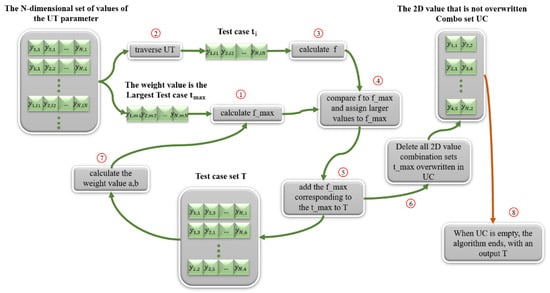
Figure 3.
The ES(a,b) algorithm generates a methodological flowchart of the test case process.
Finally, the pseudo-code form of the ES(a,b) algorithm implementation is given, as shown in Algorithm 1.
| Algorithm 1 ES(a,b) algorithm pseudocode |
|
4. Methods for Generating Functional Test Scenarios
From the discrete processing of the self-vehicle speed values in Figure 2, it can be seen that the test case set generated by the ES(a,b) algorithm has continuous values for the subelements under the traffic participant element in each test case, for example, the self-vehicle speed value of 40 represents the self-vehicle speed value interval of (30 m/h, 40 km/h), so the generated test cases cannot be used as scenarios for automatic driving simulation tests. Therefore, the generated test case cannot be used as a scenario for the simulation test of autonomous driving, and it is necessary to conduct secondary sampling of these elements to generate specific values and obtain specific scenarios before conducting the simulation test.
4.1. Monte Carlo Method
Monte Carlo Simulation (MC) is a stochastic simulation method that uses repetitive random sampling to derive numerical results [26]. MC methods include constructing or describing probabilistic processes, sampling from known probability distributions, and obtaining results through computation or simulation. Constructing or describing a probabilistic process means randomizing the parameters, for example, describing the values of the four elements under the ODD “elements in vehicle operation” as a probability distribution in the above section. After constructing the probability model, sampling from the known probability distribution is required, and the usual sampling methods include receive-reject sampling, importance sampling, Markov Monte Carlo sampling, etc. The results are obtained by performing calculations or simulations after sampling from the distribution [27].
The focus of the Monte Carlo method is to calculate the expectation of a random variable [28]. Assuming that X represents a random variable that obeys the probability distribution , then to calculate the mathematical expectation of function , it is necessary to take consecutive samples from , and then take the average of these samples of function to approximate the mathematical expectation of , as expressed in Equation (13).
where is the sample, is the function of the sample, n is the number of samples, and is the mathematical expectation of obtained by estimating the sample.
For all possible test scenarios of the autopilot function, with denoting the sample space, denoting a hazardous scenario that occurs less frequently but triggers the autopilot function, and , then the function describing whether scenario occurs can be defined as:
The probability of occurrence of scenario needs to be estimated, that is, to find . For such hazardous scenarios, which are usually located at both ends of the probability distribution of the functional test scenario parameters, the sampling yields very few hazardous accident scenarios with large variance in . This requires more sampling to reduce the variance and leads to computational overload [29].
4.2. Dangerous Scenario Clustering
Most of the sub-element fetches under the traffic participant elements generated using the Monte Carlo method are similar, which will result in a more repetitive and less efficient test if they are directly used as fetches for specific scenarios. Therefore, the group of element fetches needs to be filtered again to find out the most representative fetches, to improve the efficiency of the test. In this paper, a clustering algorithm is used for screening.
Clustering algorithm is an unsupervised machine learning algorithm, mainly used for data partitioning and data grouping in data mining, the purpose of clustering is to group similar objects in the data into one group. k-means algorithm belongs to division clustering algorithm, by clustering an n-dimensional vector of data point set , where denotes the i-th data point in the data point set, and finally dividing this data point set D into k class clusters [30]. The main basis for classifying the class clusters is the similarity of objects in the point set and the gap between objects, using Euclidean distance as the similarity measure and the error sum of squares as the objective function, and the data points are finally divided into k clusters by minimizing the objective function. In this paper, the final cluster center coordinates represent the values taken for the subelements under the traffic participant element within the specific scenario generated by each test case.
The Euclidean distance between point x and point y in the data set is:
The basic steps of the K-means algorithm are: the first step is to select k data as the initial cluster centers; the second step is to classify the data points, calculate the Euclidean distance for each point to the initial cluster center, find the cluster center with the closest Euclidean distance to each point, and divide each point under this cluster center; the third step is to check whether the cluster center to which the data points belong has changed, if not, then the clustering is finished, otherwise go to the fourth step; the fourth step is to update the cluster center coordinates, calculate the mean value for all data points under each cluster center as the new cluster center, and then skip to the second step [31].
5. Automatic Driving Function Test Scenario Generation and Simulation Test Analysis
In this paper, the function to be tested for autonomous driving is selected, and the functional test scenario generation method introduced above is used to generate simulation scenarios, and simulation software is used to conduct simulation tests, thus proving the effectiveness of the scenarios obtained based on the generation method in this paper.
5.1. Functional Test Specific Scenario Generation
Advanced Driving Assistance System (ADAS) is an intelligent system that uses a variety of on-board sensors to collect environmental information, road network information, road facilities, and road participants while the vehicle is in motion, and then realizes the alert of impending danger through the system calculation and analysis. ADAS has been widely cited at the L1 and L2 levels of autonomous driving.
Autonomous Emergency Braking (AEB), is one of the most widely used ADAS functions on L2 autonomous vehicles. In this paper, we take the AEB function as an example to generate a specific scenario for simulation testing of the AEB function. Firstly, it is necessary to construct an ODD that complies with the test regulations of the AEB function.
In 2014, Euro-NCAP released a test standard for the AEB systems, which specifies two test methods and evaluation criteria for automatic emergency braking, including automatic emergency braking for vehicle-to-vehicle (C2C) and automatic emergency braking for vehicles and vulnerable road users such as pedestrians, autonomous vehicles, and VRU [32]. Among them, the evaluation criteria of the AEB testing for vehicle-to-vehicle (C2C) mainly focus on the scenario where the test vehicle is rear-ended with the target vehicle, i.e., the front vehicle. There are three scenarios, Car-to-Car Stationary (CCRs), Car-to-Car Moving (CCRm), and Car-to-Car Braking (CCRb), depending on the movement state of the vehicle in front.
According to relevant statistics [33], the car shop rear-end scenario is one of the most dominant scenarios in current traffic accidents, so this paper selects the car shop automatic emergency braking scenario in the AEB function for design.
The AEB function test ODD is shown in Table 3. The sub-element values under the traffic participant element are discretized as continuous values, and each value represents an interval. For example, the self-driving speed value of 40 represents a value interval of (30 km/h, 40 km/h).
Table 3.
The values of each element of the ODD of the AEB function.
The weight values of ODD elements are obtained by the calculation method of scene element fetching weight values in Section 2, as shown in Table 4.
Table 4.
AEB function ODD weight value index of all elements and their values.
The AEB function ODD element values and their weight values are used as the input parameters and their weight values of the improved combination testing algorithm, and the ES(a,b) algorithm is used to generate test case sets covering dimensions n = 2, n = 3, n = 4, n = 5. To show the generation effect of ES(a,b) algorithm, this paper selects currently available combination testing tools or combination testing open source code, such as PICT, AllPairs, AETG [34]; and uses the same AEB function ODD elements as input parameters of the algorithm to generate test case sets. The number of test cases in the test case set generated by different algorithms is shown in Table 5.
Table 5.
Number of use cases generated by different combined testing algorithms in different coverage dimensions.
From Table 4, it can be seen that the ES(a,b) algorithm can effectively reduce the effect of test case generation at both lower coverage dimensions and higher coverage dimensions, so the optimization effect of ES(a,b) algorithm for test case generation has been verified.
The specific scenario generation method is used for sampling the four sub-element value intervals for each test case traffic participant element within the set of test cases with various coverage dimensions obtained by the ES(a,b) algorithm in order to obtain specific scenarios.
Take one test case in the two-dimensional combined coverage test case set generated by the ES(a,b) algorithm as an example, the four subelements under the traffic participant element of this test case have the values shown in Table 6.
Table 6.
Elements compare of the wheel and body acceleration.
Using the Monte Carlo method and clustering algorithm, the obtained post-clustering elements take values as shown in Table 7.
Table 7.
Grouping of values for clustered elements.
5.2. Automatic Driving MIL Test Based on AEB Function
As can be seen from the above, the automatic driving simulation test is divided into four types according to the test method: SIL, MIL, HIL, and HIL, and the MIL test method is chosen in this paper.
The automated driving simulation test relies on simulation software, and the automated driving virtual simulation software is a three-dimensional graphics processing software developed based on virtual reality technology [35]. The automated driving simulation test platform established based on the simulation software needs to have the ability to truly restore standard regulatory test scenes and transform the road collection data of real vehicles to generate simulation scenes, while the simulation test platform should realize that vehicles can be carried out in the platform cloud At the same time, the simulation test platform should realize the ability of large batch and parallel simulation of vehicles in the platform cloud; so that the simulation test can realize the closed-loop test of the full-stack algorithm of automatic driving perception, planning, decision making and control.
This paper uses PreScan, a simulation software for driver assistance system and safety system development and validation, whose main functions include scenario building, sensor modeling, developing control algorithms and running simulation [36]. Compared with VTD, CarSim, Carla, and other simulation software, the advantages of PreScan are a simple scenario modeling process, perfect sensor and vehicle dynamics model, and PreScan is equipped with an interface for joint simulation with Matlab/Simulink, through which control and decision making algorithms in Matlab/Simulink can be imported. algorithms, and also in Matlab/Simulink to modify the vehicle dynamics model and demo algorithms that come with PreScan [37]. In this paper, the specific scenario of Table 7 is selected for simulation testing, and the ODD elements of the specific scenario of Table 7 are taken as shown in Table 8.
Table 8.
In Table 7, the ODD road and environment elements are selected for specific scenarios.
The simulation scenario generated by PreScan is shown in Figure 4.
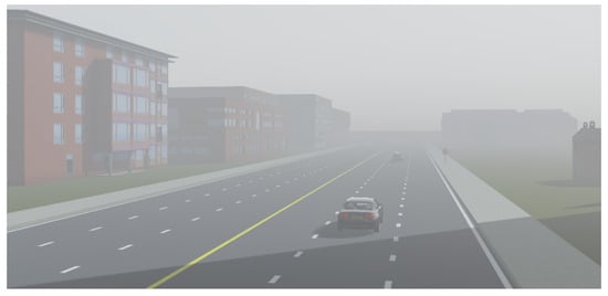
Figure 4.
AEB simulation tests scenarios.
Add a long-range millimeter wave radar to the self-vehicle in PreScan, set FoV as a pyramidal, single beam, scanning frequency 25 Hz, detection distance 150 m, lateral FoV opening angle 9 degrees, with a maximum number of detected targets of 32, and leave the rest parameters as the default parameters.
Add short-range millimeter wave radar, set FoV as pyramidal, single beam, scanning frequency 25 Hz, detection distance 30 m, lateral FoV opening angle 90 degrees, maximum number of detected targets 32, and the rest parameters as default parameters.
Click “build” to compile, and after compiling, open the corresponding .slx file in simulink and complete the connection of each module input and output. In this paper, we choose Prescan’s own AEB control algorithm, which uses the time to collision (TTC) as the judgment criterion. When TTC < 2.6 s, the control algorithm gives an alarm signal; when TTC < 1.6 s, the control algorithm gives about 40% of the half braking signal; when TTC < 0.6 s, the control algorithm gives about 100% of the full braking signal.
The added sensor model, dynamics model, and AEB control algorithm are the same for both scenarios. When you click “Run Simulation”, you can see the two windows added with the vehicle view, the real-time motion status window of the vehicle, and the window showing the sensing results of the millimeter wave radar, as shown in Figure 5.
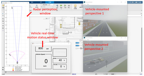
Figure 5.
PreScan simulation runs each window interface.
At the end of the simulation run, the graphs of the change of the speed of the self-vehicle and can be obtained for the relative distance between the self-vehicle and the target vehicle, as shown in Figure 6. The horizontal coordinate in the graph represents the simulation running time, the red curve represents the relative distance between two vehicles, and the blue curve represents the speed of the self-vehicle.
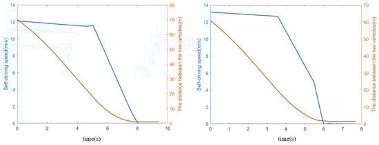
Figure 6.
Simulate and test the results of each indicator parameter.
As can be seen from Figure 6, in Scenario 1 at the start of the simulation, the two cars are 74.43 m apart, the self-car monitors the target car, and the self-car travels straight at a constant speed of 43.63 km/h or 12.12 m/s; when the two cars are about 18 m apart, the AEB system gives a full brake and the self-car comes to a stop; after the brakes stop the two cars are about 1 m apart and the self-car’s braking time is 2.7 s.
Scenario 2 At the beginning of the simulation, the two cars were 65.21 m apart, the self-car monitors the target car, the self-car goes straight at a constant speed of 47.40 km/h or 13.17 m/s; when the distance between the two cars is about 19 m, the AEB system gives a full brake and the self-car comes to a stop; the distance between the two cars after braking is about 1.5 m, and the braking time of the self-car is 2.2 s.
From the simulation results, it can be seen that the AEB control algorithm and the millimeter wave radar used in the simulation test performed well under bad weather conditions of sand and haze, when the speed range of the self-car was (40 km/h, 60 km/h), and the self-car braked at about a 1–2 m distance between the two cars to avoid the accident.
To test the effect of the AEB function when the speed of the self-car is high under the same sandy haze weather conditions, this paper selects another test case in the two-dimensional combined coverage test case set generated by the ES(a,b) algorithm for the testing. The specific scenario is generated by this test case is shown in Table 9.
Table 9.
Specific scenarios generated by the test cases.
Add the sensor model, vehicle dynamics model and AEB control algorithm consistent with the above. Run the simulation and get the variation graphs for self-vehicle speed, relative distance between self-vehicle and the target vehicle and self-vehicle braking-force parameters, as shown in Figure 7.
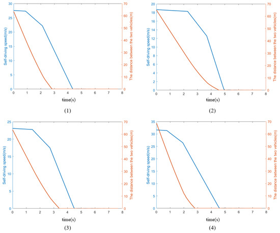
Figure 7.
Simulate and test the results of each indicator parameter. (1–4) Specific scenarios for MIL testing of AEB function.
At the beginning of Simulation Scenario 1, the speed of the self-car is 99.29 km/h or 27.58 m/s, and the distance between the self-car and the target car is 67.89 m; when the distance between the two cars is about 40 m, the AEB control algorithm controls the self-car to give about 40% of braking force; when the distance between the two cars is about 10 m, the AEB control algorithm controls the self-car to give 100% of full braking force; when the distance between the two cars is 0 m, the self-car When the distance between the two cars is 0 m, the speed is about 16 m/s, the self-car is not being braked, and the two cars collide. Since the collision animation effect is not set, the animation shown is that the target car passes through the self-car, and then the self-car brakes to stop.
At the beginning of simulation scenario 2, the speed of the self-car is 67.26 km/h or 18.68 m/s, and the distance between the self-car and the target car is 69.30 m; when the distance between the two cars is about 38 m, the AEB control algorithm controls the self-car to give about 40% braking force; when the distance between the two cars is about 10 m, the AEB control algorithm controls the self-car to give 100% full braking force; when the distance between the two cars is 0 m, the self-car’s speed is about 15 m/s, the self-car is not braked, and the two cars collide.
At the beginning of simulation scenario 3, the speed of the self-car is 83.07 km/h or 23.08 m/s, and the distance between the self-car and the target car is 67.84 m; when the distance between the two cars is about 32 m, the AEB control algorithm controls the self-car to give about 40% braking force; when the distance between the two cars is about 9 m, the AEB control algorithm controls the self-car to give 100% full braking force; when the distance between the two cars is 0 m, the speed of the self-car is When the distance between the two cars is 0 m, the speed of the self-car is about 11m/s, the self-car is not braked, and the two cars collide.
At the beginning of simulation scenario 4, the speed of the self-car is 113.87 km/h or 31.63 m/s, and the distance between the self-car and the target car is 73.13 m; when the distance between the two cars is about 42 m, the AEB control algorithm controls the self-car to give about 40% braking force; when the distance between the two cars is about 13m, the AEB control algorithm controls the self-car to give 100% full braking force; when the distance between the two cars is 0 m, the self-car When the distance between the two cars is 0 m, the speed is about 18 m/s, the self-car is not braked, and the two cars collide.
From the simulation results, it can be seen that under the bad weather conditions of sand and haze, the AEB control algorithm and the millimeter wave radar used in the simulation test performed poorly when the speed range of the self-car was (60 km/h,120 km/h), and the AEB control algorithm did not apply direct full braking, but instead provided half braking initially and then full braking. This resulted in a collision between the two cars when they were 0 m apart, and the autonomous vehicle did not brake.
In summary, the validity of the specific scenarios obtained above for MIL testing of AEB functions has been verified.
6. Conclusions
Aiming at the problems of a lack of real data support, low generation efficiency, and a lack of dangerous scenes in the scene element parsing and reorganization of the scene generation method in the autonomous driving virtual simulation test scene generation method, this paper proposes an autonomous driving virtual simulation scene generation method that can take into account the importance of the scene elements in the real world, optimize the number of scene generation and generate dangerous specific scenes. Based on this, an autonomous driving MIL test platform is built with PreScan and Matlab/Simulink to verify the effectiveness of the scenario generation method through simulation testing of ADAS functions. The method can be used to generate test scenarios for all functions of L2-level ADAS for autonomous driving, and can also generate simulation scenarios required for scenario testing and task testing. In the future, when the laws and regulations for L3 and above autonomous driving tests are perfected, the scenario generation method proposed in this paper only needs to improve the structure of ODD elements and more detailed divisions; and can be used for the generation of L3 and above autonomous driving simulation test scenarios.
However, the method still has certain limitations and problems, which need further research and improvement. The main areas include the following:
(1) The method of scene element analysis and scene reorganization is used to generate scenes, and although the weight values of ODD element values are calculated by referring to real statistics, the support of traffic accident data is lacking. Therefore, in the future, traffic accident data should be introduced into the calculation of the weight value of the ODD elements, and the distribution of the elements in the road conditions, environmental conditions, and the vehicle operation state when the real accident scenes occur should be analyzed to assign weights to the ODD elements, so as to improve the realism of the generated scenes.
(2) The improved combination test algorithm based on the weight values of ODD element taking values has a longer generation time and lower efficiency at higher coverage dimensions. Therefore, future research should consider introducing machine learning and reinforcement learning methods into scene generation methods in order to design optimized objective functions for generate scenes; in addition, subsequent research can use optimization algorithms, such as random number search algorithms, particle swarm optimization algorithms, simulated annealing algorithms, and other algorithms for quickly converging to the global optimal solution in order to find dangerous scenarios.
Author Contributions
Conceptualization, N.L. and L.C.; methodology, N.L.; software, Y.H.; validation, N.L., L.C. and Y.H.; formal analysis, N.L.; investigation, N.L.; resources, N.L., L.C. and Y.H.; data curation, N.L.; writing—original draft preparation, N.L.; writing—review and editing, N.L. and L.C.; supervision, L.C.; project administration, L.C. All authors have read and agreed to the published version of the manuscript.
Funding
This research received no external funding.
Data Availability Statement
The data described in this study are available within the article.
Conflicts of Interest
The authors declare no conflict of interest. Yongchao, Huang is employee of Shanghai Waylancer Automotive Technology Co., Ltd. The paper reflects the views of the scientists, and not the company.
References
- Kalra, N.; Paddock, S.M. Driving to safety: How many miles of driving would it take to demonstrate autonomous vehicle reliability? Transp. Res. Part Policy Pract. 2016, 94, 182–193. [Google Scholar] [CrossRef]
- Menzel, T.; Bagschik, G.; Maurer, M. Scenarios for Development, Test and Validation of Automated Vehicles. In Proceedings of the 2018 IEEE Intelligent Vehicles Symposium (IV), Suzhou, China, 26–30 June 2018. [Google Scholar]
- Chen, W.; Kloul, L. An Ontology-Based Approach to Generate the Advanced Driver Assistance Use Cases of Highway Traffic. In Proceedings of the 10th International Conference on Knowledge Engineering and Ontology Development, Seville, Spain, 18–20 September 2018; pp. 75–83. [Google Scholar]
- Li, Y.; Tao, J.; Wotawa, F. Ontology-based test generation for automated and autonomous driving functions. Inf. Softw. Technol. 2020, 117, 106200. [Google Scholar] [CrossRef]
- Gao, F.; Duan, J.; He, Y.; Wang, Z. A Test Scenario Automatic Generation Strategy for Intelligent Driving Systems. Math. Probl. Eng. 2019, 2019, 3737486. [Google Scholar] [CrossRef]
- Gao, F.; Duan, J.; Han, Z.; He, Y. Automatic Virtual Test Technology for Intelligent Driving Systems Considering Both Coverage and Efficiency. IEEE Trans. Veh. Technol. 2020, 69, 14365–14376. [Google Scholar] [CrossRef]
- Lee, R.; Kochenderfer, M.J.; Mengshoel, O.J.; Brat, G.P.; Owen, M.P. Adaptive stress testing of airborne collision avoidance systems. In Proceedings of the 2015 IEEE/AIAA 34th Digital Avionics Systems Conference (DASC), Prague, Czech Republic, 13–17 September 2015; pp. 1–24. [Google Scholar]
- Koren, M.; Alsaif, S.; Lee, R.; Kochenderfer, M.J. Adaptive Stress Testing for Autonomous Vehicles. In Proceedings of the 2018 IEEE Intelligent Vehicles Symposium (IV), Suzhou, China, 26–30 June 2018; pp. 1–7. [Google Scholar]
- Alexiadis, V.; Colyar, J.; Halkias, J.; Hranac, R.; McHale, G. The next generation simulation program. ITE J. (Inst. Transp. Eng.) 2004, 74, 22–26. [Google Scholar]
- Demetriou, A.; Alfsvåg, H.; Rahrovani, S.; Chehreghani Haghir, M. A Deep Learning Framework for Generation and Analysis of Driving Scenario Trajectories. SN Comput. Sci. 2023, 4, 251–267. [Google Scholar] [CrossRef]
- Ding, W.; Wang, W.; Zhao, D. A Multi-Vehicle Trajectories Generator to Simulate Vehicle-to-Vehicle Encountering Scenarios. In Proceedings of the 2019 International Conference on Robotics and Automation (ICRA), Montreal, QC, Canada, 20–24 May 2019; pp. 4255–4261. [Google Scholar]
- Termöhlen, J.-A.; Bär, A.; Lipinski, D.; Fingscheidt, T. Towards Corner Case Detection for Autonomous Driving. In Proceedings of the 2019 IEEE Intelligent Vehicles Symposium (IV), Paris, France, 9–12 June 2019; pp. 438–445. [Google Scholar]
- Ries, L.; Langner, J.; Otten, S.; Bach, J.; Sax, E. A Driving Scenario Representation for Scalable Real-Data Analytics with Neural Networks. In Proceedings of the 2019 IEEE Intelligent Vehicles Symposium (IV), Paris, France, 9–12 June 2019. [Google Scholar]
- Zhang, S.; Peng, H.; Zhao, D.; Tseng, H.E. Accelerated Evaluation of Autonomous Vehicles in the Lane Change Scenario Based on Subset Simulation Technique. In Proceedings of the 2018 21st International Conference on Intelligent Transportation Systems (ITSC), Maui, HI, USA, 4–7 November 2018; pp. 3935–3940. [Google Scholar]
- Li, L.; Lin, Y.L.; Zheng, N.N.; Wang, F.Y.; Liu, Y.; Cao, D.; Wang, K.; Huang, W.L. Artificial intelligence test: A case study of intelligent vehicles. Artif. Intell. Rev. 2018, 50, 441–465. [Google Scholar] [CrossRef]
- Zimmerman, M. Empowerment Theory. In Handbook of Community Psychology; Springer: Boston, MA, USA, 2012. [Google Scholar] [CrossRef]
- Ye, F.-F.; Yang, L.-H.; Wang, Y.-M. A new environmental governance cost prediction method based on indicator synthesis and different risk coefficients. J. Clean. Prod. 2019, 212, 548–566. [Google Scholar] [CrossRef]
- Cattaneo, L.; Chapman, A. The Process of Empowerment A Model for Use in Research and Practice. Am. Psychol. 2010, 65, 646–659. [Google Scholar] [CrossRef]
- Krishnan, A.R.; Kasim, M.M.; Hamid, R.; Ghazali, M.F. A Modified CRITIC Method to Estimate the Objective Weights of Decision Criteria. Symmetry 2021, 13, 973. [Google Scholar] [CrossRef]
- Diakoulaki, D.; Mavrotas, G.; Papayannakis, L. Determining objective weights in multiple criteria problems: The critic method. Comput. Oper. Res. 1995, 22, 763–770. [Google Scholar] [CrossRef]
- Pedrycz, W.; Song, M. Analytic Hierarchy Process (AHP) in Group Decision Making and its Optimization with an Allocation of Information Granularity. IEEE Trans. Fuzzy Syst. 2011, 19, 527–539. [Google Scholar] [CrossRef]
- Ahmed, F.; Kilic, K. Fuzzy Analytic Hierarchy Process: A performance analysis of various algorithms. Fuzzy Sets Syst. 2019, 362, 110–128. [Google Scholar] [CrossRef]
- Zhang, Q.; Chen, D.; Li, Y.; Li, K. Research on Performance Test Method of Lane Departure Warning System with PreScan. In Proceedings of SAE-China Congress 2014: Selected Papers; Springer: Berlin/Heidelberg, Germany, 2015; pp. 445–453. [Google Scholar]
- Ahmed, B.S.; Zamli, K.Z. A variable strength interaction test suites generation strategy using Particle Swarm Optimization. J. Syst. Softw. 2011, 84, 2171–2185. [Google Scholar] [CrossRef]
- Calò, A.; Arcaini, P.; Ali, S.; Hauer, F.; Ishikawa, F. Generating Avoidable Collision Scenarios for Testing Autonomous Driving Systems. In Proceedings of the 13th IEEE International Conference on Software Testing, Validation and Verification (ICST), Porto, Portugal, 24–28 October 2020. [Google Scholar]
- Drews, T. Monte Carlo Simulation of Kinetically Limited Electrodeposition on a Surface with Metal Seed Clusters. Z. Fur Phys.-Chem.-Int. J. Res. Phys. Chem. Chem. Phys.-Phys. Chem. 2007, 221, 1287–1305. [Google Scholar] [CrossRef]
- Sarrut, D.; Etxebeste, A.; Munoz, E.; Krah, N.; Létang, J.M. Artificial Intelligence for Monte Carlo Simulation in Medical Physics. Front. Phys. 2021, 9, 738112. [Google Scholar] [CrossRef]
- Qazi, A.; Shamayleh, A.; El-Sayegh, S.; Formaneck, S. Prioritizing risks in sustainable construction projects using a risk matrix-based Monte Carlo Simulation approach. Sustain. Cities Soc. 2020, 65, 102576. [Google Scholar] [CrossRef]
- Mallongi, A.; Rauf, A.U.; Daud, A.; Hatta, M.; Al-Madhoun, W.; Amiruddin, R.; Stang, S.; Wahyu, A.; Astuti, R.D.P. Health risk assessment of potentially toxic elements in Maros karst groundwater: A Monte Carlo simulation approach. Geomat. Nat. Hazards Risk 2022, 13, 338–363. [Google Scholar] [CrossRef]
- Sinaga, K.; Yang, M.-S. Unsupervised K-Means Clustering Algorithm. IEEE Access 2020, 6, 80716–80727. [Google Scholar] [CrossRef]
- Ahmed, M.; Seraj, R.; Islam, S. The k-means Algorithm: A Comprehensive Survey and Performance Evaluation. Electronics 2020, 9, 1295. [Google Scholar] [CrossRef]
- Dollorenzo, M.; Dodde, V.; Giannoccaro, N.I.; Palermo, D. Simulation and Post-Processing for Advanced Driver Assistance System (ADAS). Machines 2022, 10, 867. [Google Scholar] [CrossRef]
- Pal, C.; Narahari, S.; Vimalathithan, K.; Manoharan, J.; Hirayama, S.; Hayashi, S.; Combest, J. Real World Accident Analysis of Driver Car-to-Car Intersection Near-Side Impacts: Focus on Impact Location, Impact Angle and Lateral Delta-V; WCX World Congress Experience: London, UK, 2018. [Google Scholar]
- Cohen, D.M.; Dalal, S.R.; Fredman, M.L.; Patton, G.C. The AETG system: An approach to testing based on combinatorial design. IEEE Trans. Softw. Eng. 1997, 23, 437–444. [Google Scholar] [CrossRef]
- Nalić, Đ.; Pandrevic, A.; Eichberger, A.; Rogic, B. Design and Implementation of a Co-Simulation Framework for Testing of Automated Driving Systems. Sustainability 2020, 12, 10476. [Google Scholar] [CrossRef]
- Ortega, J.; Lengyel, H.; Szalay, Z. Overtaking maneuver scenario building for autonomous vehicles with PreScan software. Transp. Eng. 2020, 2, 100029. [Google Scholar] [CrossRef]
- Wang, C.-S.; Liu, D.-Y.; Hsu, K.-S. Simulation and application of cooperative driving sense systems using prescan software. Microsyst. Technol. 2021, 27, 1201–1210. [Google Scholar] [CrossRef]
Disclaimer/Publisher’s Note: The statements, opinions and data contained in all publications are solely those of the individual author(s) and contributor(s) and not of MDPI and/or the editor(s). MDPI and/or the editor(s) disclaim responsibility for any injury to people or property resulting from any ideas, methods, instructions or products referred to in the content. |
© 2023 by the authors. Licensee MDPI, Basel, Switzerland. This article is an open access article distributed under the terms and conditions of the Creative Commons Attribution (CC BY) license (https://creativecommons.org/licenses/by/4.0/).