1. Introduction
The world’s energy consumption structure has been dominated by fossil energy for a long time, and annual global coal consumption accounts for 30% of energy consumption [
1]. To meet the demand for coal, improve the safety, efficiency, and environmental protection of coal mining, and realize the automation and intelligence of mining machinery [
2,
3] is an inevitable development trend.
2. Literature Review
The path tracking control technology of transportation vehicles in open-pit mines is one of the cores of intelligent coal mining technology. In this regard, academia and industry have carried out research on minecart path tracking control and achieved some research results. This method [
4] adopted the path preview-tracking method to decouple the lateral control from the vertical control and corrected the deviation in real time through the feedback mechanism, realizing the lateral and vertical control of the unmanned mining transport vehicle. Choi et al. [
5] compared a sliding mode control (SMC) with a driver model-based controller consisting of a PI controller with a preview distance. SMC has higher path tracking accuracy but requires larger steering input. Bai, G. [
6] used the MPC based on the preview distance combined with the preview method to judge the sudden change of road curvature in advance and MPC to handle the characteristics of multi-variable and multi-constraint system control, which improved the path tracking accuracy of the underground mining articulated vehicle. Lima et al. [
7] proposed an adaptive preview distance determination method based on fuzzy control, taking the intelligent combine harvester as the research object. The path tracking algorithm should adaptively adjust the size of the preview distance according to the speed and other states of the harvester. Fuzzy control does not depend on a specific model and can better deal with the problem of dynamic adjustment of the harvester’s preview distance under different operating conditions and improve the adaptability of the path tracking algorithm. Xu, S. et al. [
8] distinguished forward lateral control and reverse lateral control in the lateral control algorithm of mining trucks, using the center of the front axle and the center of the rear axle as reference points, respectively, and adopted an adaptive preview method based on speed and curvature, realize lateral control on complex road surfaces in mining areas. Lima et al. [
9] deduced the vehicle error kinematics model in the time domain to the space domain in the Frenet coordinate system and tested it on a Scania truck to verify that it can output a smoother output than the pure tracking controller. However, it does not consider that the truck has a steering mechanism with large inertia, so that there is a delay link in the control, which will reduce the performance of the controller.
However, the working environment of open-pit mine transportation vehicles is harsh, and there are areas such as bumpy roads, large undulating ramps, and narrow U-turn sections on the road. In addition, the vehicle has problems with a large delay in steering actuators and poor response accuracy, which causes path tracking control serpentine form and large deviation of lateral tracking [
10]. Because MPC can better consider the actuator delay compensation and solve the problems of steering oscillation and instability, it becomes a better control method. The following research [
6,
8,
10] guides the design direction and content of this paper. By establishing a vehicle kinematics model that considers the system delay link, and based on the model, the MPC controller is designed, and the simulation verification and performance comparison of the controller is carried out. Finally, a real vehicle test is carried out in the Shenyan Xiwan Coal Mine to verify the proposed method. The results show that the MPC controller considering the delay characteristics of system has better control performance than the traditional Stanley control in both simulation and real vehicle test environments.
3. Comparison of Path Tracing Methods
Many scholars at home and abroad have studied the path tracking technology of vehicles and achieved many research results. The commonly used path tracking methods include pure tracking control [
11,
12], Stanley control [
13,
14], model predictive control [
15,
16,
17], et al. In this section, a numerical simulation comparison of these methods is carried out, and then the method with the best performance is selected for the real vehicle experiment and test in the next section.
3.1. Pure Pursuit Control
Pure pursuit control outputs the front wheel angle of the vehicle based on the geometric relationship between the road and the vehicle so that the vehicle follows the reference path [
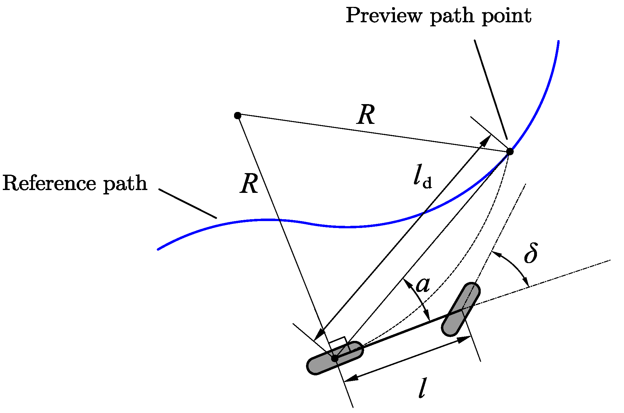
10]. Pure pursuit control has been widely used by researchers because of its simple implementation, easy parameter tuning, low computational burden, and good low-speed performance. In this technique, the target point on the reference path is chosen at a certain distance in front of the vehicle, called the “look-ahead distance”. The relationship between the vehicle position and the path trajectory is established by fitting an arc between the center of the rear wheel and the target point.
Figure 1 shows the geometry of the pure tracking method of the bicycle vehicle model. The radius of the fitted arc is as follows:
where
is the angle between the vehicle heading and the line connecting the waypoint and the center of the rear axle of the vehicle,
is the preview distance, and
is the arc radius.
Combining Equation (1) with the Ackerman steering model, the required steering angle can be calculated as [
11]:
where
is the wheelbase of the vehicle.
3.2. Stanley Control
The Stanley controller is also a geometry-based path pursuit controller [
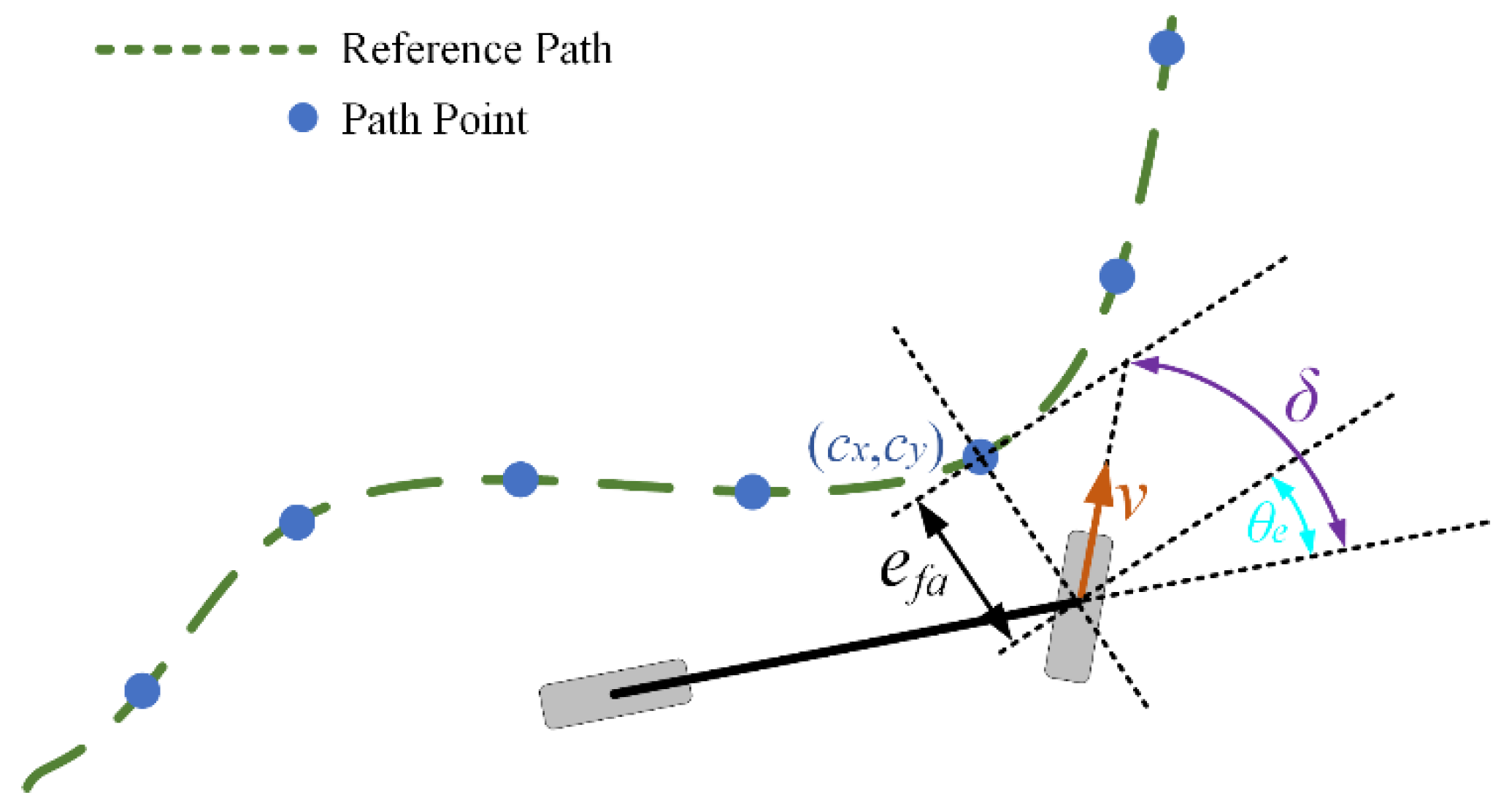
12]. The geometric relationship of the Stanley controller is shown in
Figure 2. In this figure,
is the distance between the vehicle’s front axle and the reference point and
is the angle between the vehicle’s driving direction and the tangent to the reference waypoint. From the geometric relationship in
Figure 2, the required steering angle of the front wheel of the vehicle is calculated from the two-part deviation, which is the sum of the angle deviation between the reference path point tangent and the vehicle heading and the ratio of the distance deviation to the vehicle speed [
13].
3.3. Model Predictive Control
MPC estimates the future state of the system over a certain time horizon using an explicit model of the system. At each sampling interval, the controller’s goal is to find an optimal control sequence based on the predicted state. From the optimized control sequence, only the first control action is sent to the system and the whole process is repeated for a specific time interval. MPC has several advantages for path following controllers. The main advantage of MPC is its ability to handle multi-state variables and constraints [
17]. However, its disadvantage increases the computational complexity of the controller for solving the online optimization problem. In response to this problem, some scholars have proposed related optimization speed-up solution methods, such as by Sun Hao [
18] and others who proposed an accelerated calculation method based on time-domain decomposition, which reduces the time-consuming solution to a certain extent.
MPC generally adopts two methods to design a path tracking controller; one is NMPC using a nonlinear vehicle model, and the other is linear MPC using a linear approximation model. To reduce the complexity of solving the optimization problem, we can employ different linearization techniques. When a continuous linearization method is used at each operating point, the system is transformed to a linear time-varying step. This step can be implemented on a kinematic or dynamic model [
19].
4. Design of Path Tracing Strategy Based on MPC
4.1. Vehicle Kinematics Model
Assuming that the four-wheeled-vehicle model is symmetrical about the longitudinal plane of the vehicle [
20], a two-wheeled three-degree-of-freedom vehicle model is obtained. When the vehicle is under low speed, it can be described by the kinematics formula when it is less affected by the lateral dynamics:
where
are the abscissa and ordinate of the center of the rear axle of the vehicle in the global coordinate system, respectively;
is the heading angle of the vehicle;
is the wheelbase;
is the speed of the vehicle; and
is the steering angle of the front wheel of the vehicle. The vehicle motion state information in the Cartesian coordinate system is decomposed into the Frenet coordinate system as shown in
Figure 2, which is derived from the geometric relationship:
where
is the velocity projection of the vehicle along the tangent direction of the reference path point,
is the road reference heading angular velocity,
is the curvature radius of the road,
is the lateral position deviation between the vehicle rear axle center and the reference path, and
is the vehicle heading angle and the road reference heading angle.
is the speed of the center of the rear axle of the vehicle.
The derivatives of lateral position deviation and heading angle deviation with respect to time are as follows:
where
is the actual steering angle of the vehicle, and
is the wheelbase of the vehicle.
Considering that the lateral deviation of the vehicle tracking path is negligible relative to the curvature radius of the road, and the steering angle command output by the controller and the execution command of the actuator will have a delay, the vehicle kinematics deviation model in Frenet coordinates is:
where
is the vehicle steering angle command.
Equation (3) is expressed in state space as:
State factors are .
Input is .
4.2. Linearization and Discretization of Models
To facilitate the design of the controller, Equation (7) is linearized by the first-order Taylor expansion near the reference value, and the model obtained after discretization by the bilinear method is:
Equation (8) is the derived linear time-varying prediction model, which is the basis for establishing the vehicle kinematics model prediction controller based on the Frenet coordinate system.
4.3. MPC Controller Design
The output is
,
, the prediction horizon is
. According to Equation (8), the state of the vehicle in the predicted horizon is derived as:
The cost function and constraints are the main body of the optimization problem. The cost function ensures the accuracy of the vehicle tracking path, and the constraints ensure that the steering angle control amount of the vehicle is within the maximum turning angle of the front wheel of the vehicle and does not send sudden changes to affect the stability of the path tracking. The established cost function and constraints are as follows:
where
is the output value in the prediction horizon,
is the control sequence of the input in the prediction horizon,
is weight coefficient matrix,
are the upper and lower bounds for the control constrains, respectively,
are the upper and lower bounds for the control increment constrains, respectively.
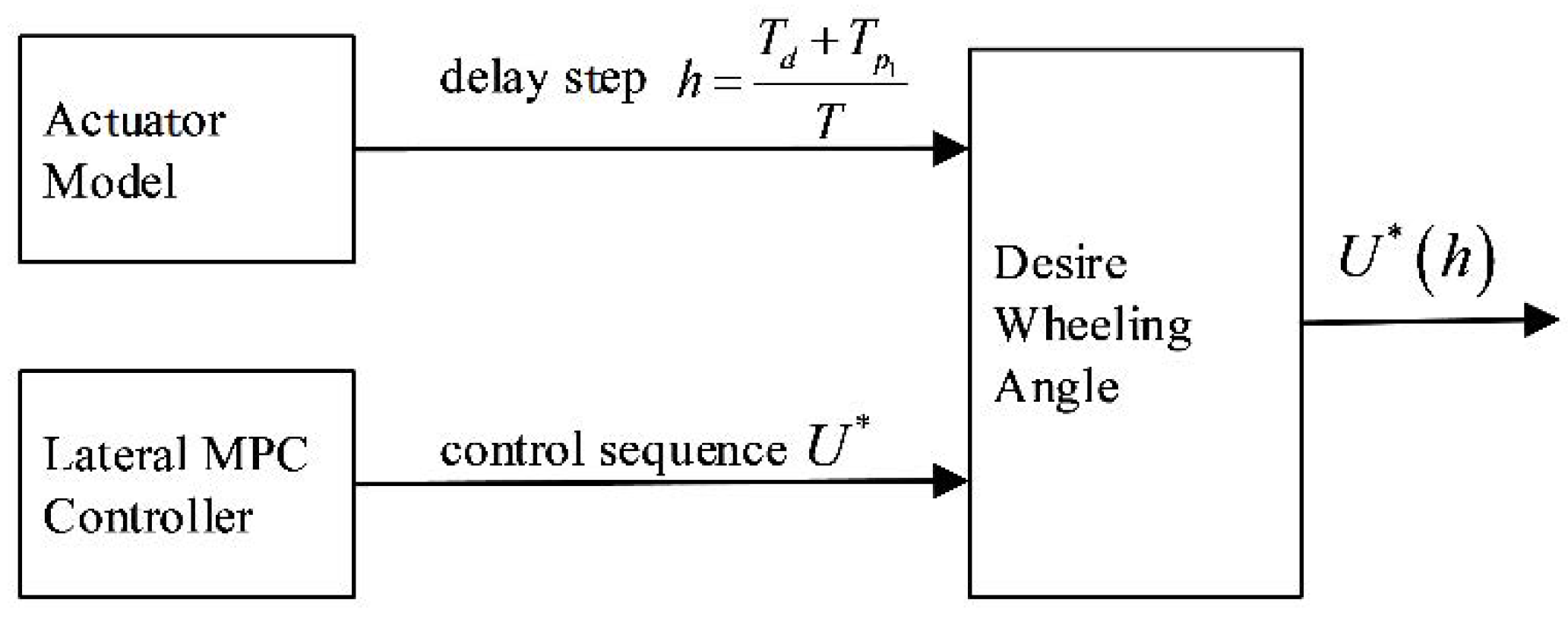
During the actual operation of the mining truck, there is a delay in the steering actuator, and it takes a period of time for the command of the controller to be executed by the actuator in place. In this paper, the application of an MPC path tracking control can predict the motion of the vehicle for a period of time into the future through the vehicle kinematic model and output the characteristics of a control sequence corresponding to each moment to deal with the influence of delay. As show in
Figure 3, in the case of considering the delay, the output control quantity is not the first control quantity in the control sequence, but the control quantity corresponding to the moment after the delay time.
4.4. Steering Actuator Model Identification
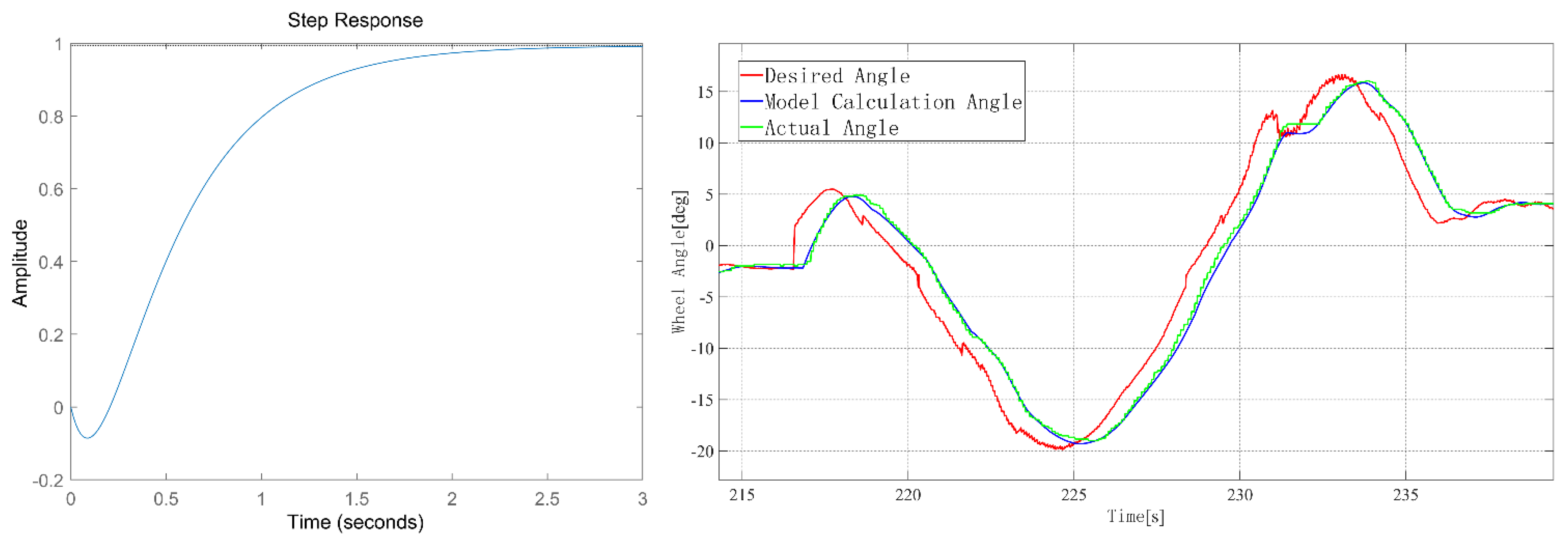
To obtain the actuator delay and gain characteristics, the actuator model is identified through experimental data. The actuator model is a first-order delay response transfer function:
The step response curve of the steering actuator is shown in
Figure 4. The actuator has a large delay link and amplitude attenuation. After compensation through the model, the actual steering curve (green) and the model calculated curve (blue) have a high degree of matching, and the steering curve calculated by the model can more accurately reflect the actual steering change.
By modeling the steering actuator, the delay and gain characteristics of the actuator itself are considered in the control system, which can effectively reduce the system control error and improve the control accuracy.
5. System Simulation Verification
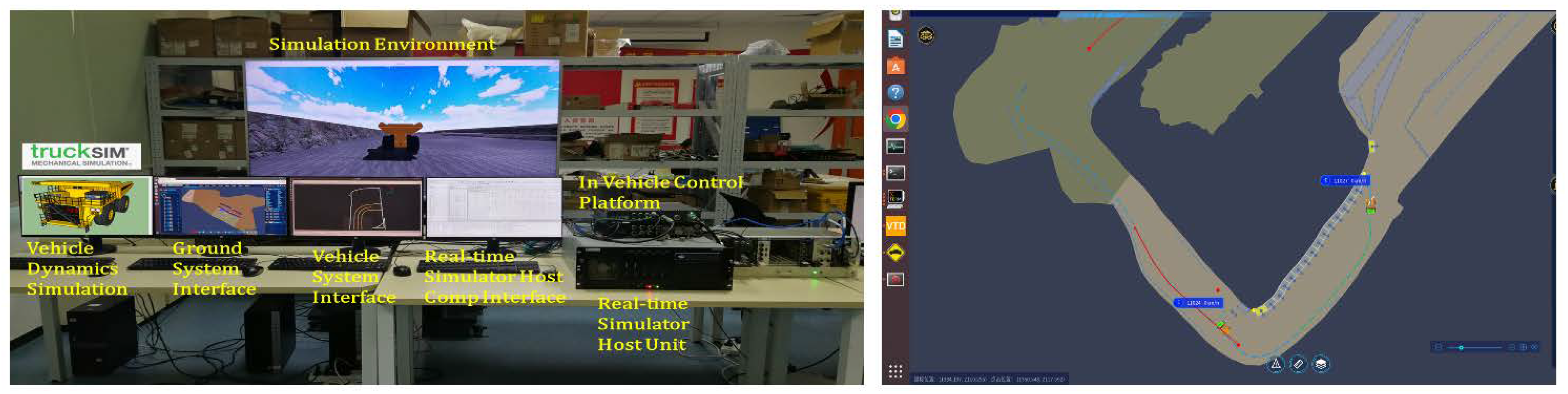
The MPC controller and the Stanley controller are simulated and verified on the hardware-in-the-loop simulation platform (as shown in
Figure 5), and the experimental results are consistent except for the lateral controller, as shown in
Figure 6,
Figure 7,
Figure 8,
Figure 9.
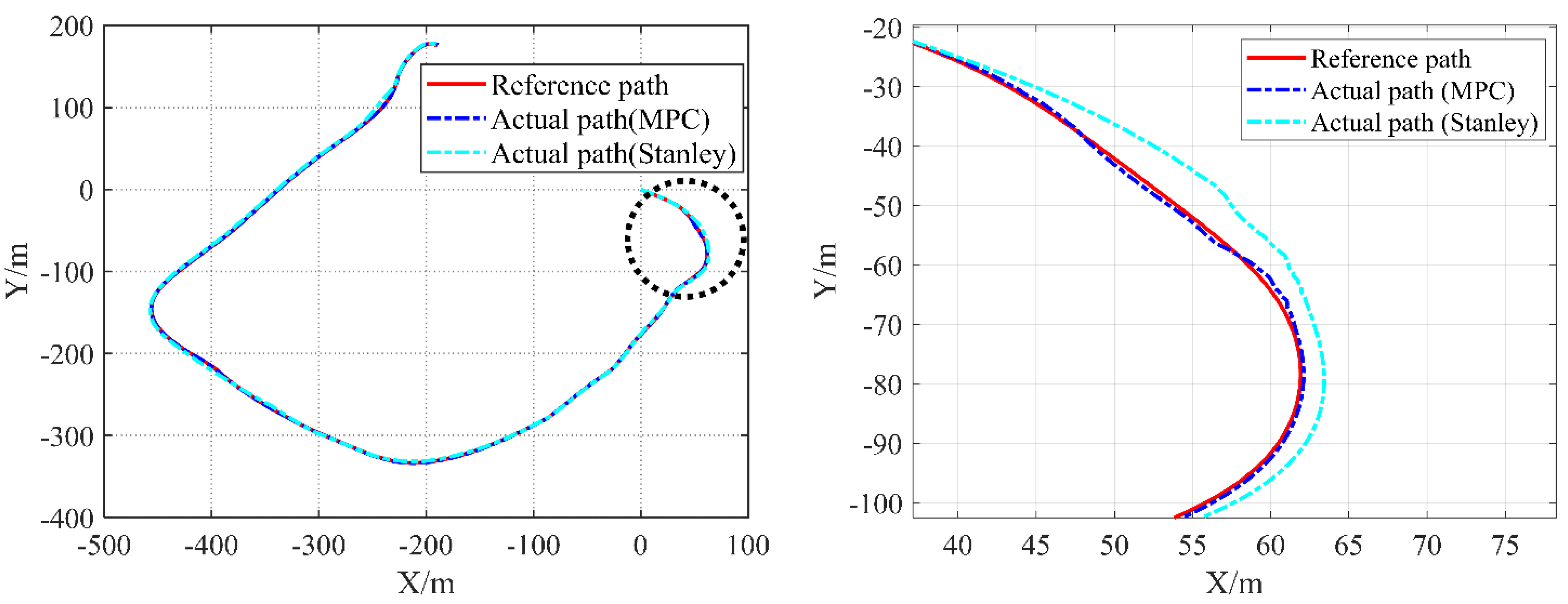
It can be seen from the above test results that under the complex working conditions of the “C” shape and “S” shape reference path, as shown in
Table 1, the MPC control algorithm has a significantly improved control effect on the lateral deviation than the Stanley algorithm, and the control effect on the heading angle deviation is comparable. Under the “C” shape reference path, the maximum lateral deviation is reduced from 1.2 to 0.6 m, and the average lateral deviation is reduced from 0.6 m to 0.2 m.
6. Real Vehicle Experiment
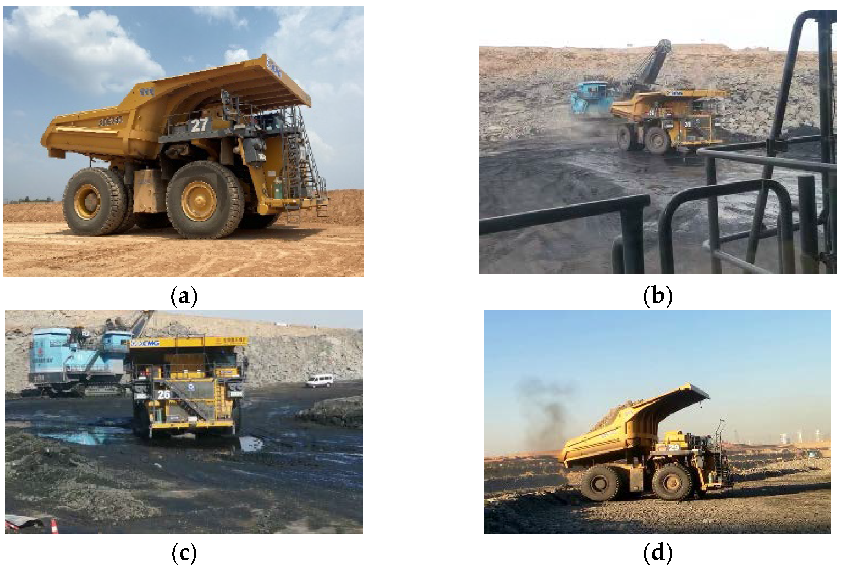
In the Xiwan Coal Mine of Shenyan, China, a real vehicle test of the control strategy proposed above was carried out, and the experimental scene is shown in
Figure 10. The wheelbase of the vehicle is 6.35 m, and the tests are carried out on the “C”-shaped reference path of 10 km/h and the “S”-shaped reference path of 20 km/h, considering that the delay of the steering gear is 0.8 s, and the maximum wheel angle is 30 degrees.
The calibration of the MPC control parameters was achieved through simulation and a large number of experiments. The relevant parameters of the model predictive controller are shown in
Table 2.
It should be noted that because the field test environment will change in real time because of the operation, and the road trajectory will be updated and adjusted accordingly, there will be differences between the simulation results and the real vehicle test results.
Under the C-shaped reference path with the average speed of 10 km/h, the maximum speed during the driving process will reach 20 km/h. For safety reasons, the reference speed of the vehicle will be limited when driving on a curve with large curvature. The vehicle speed during the test is shown in the
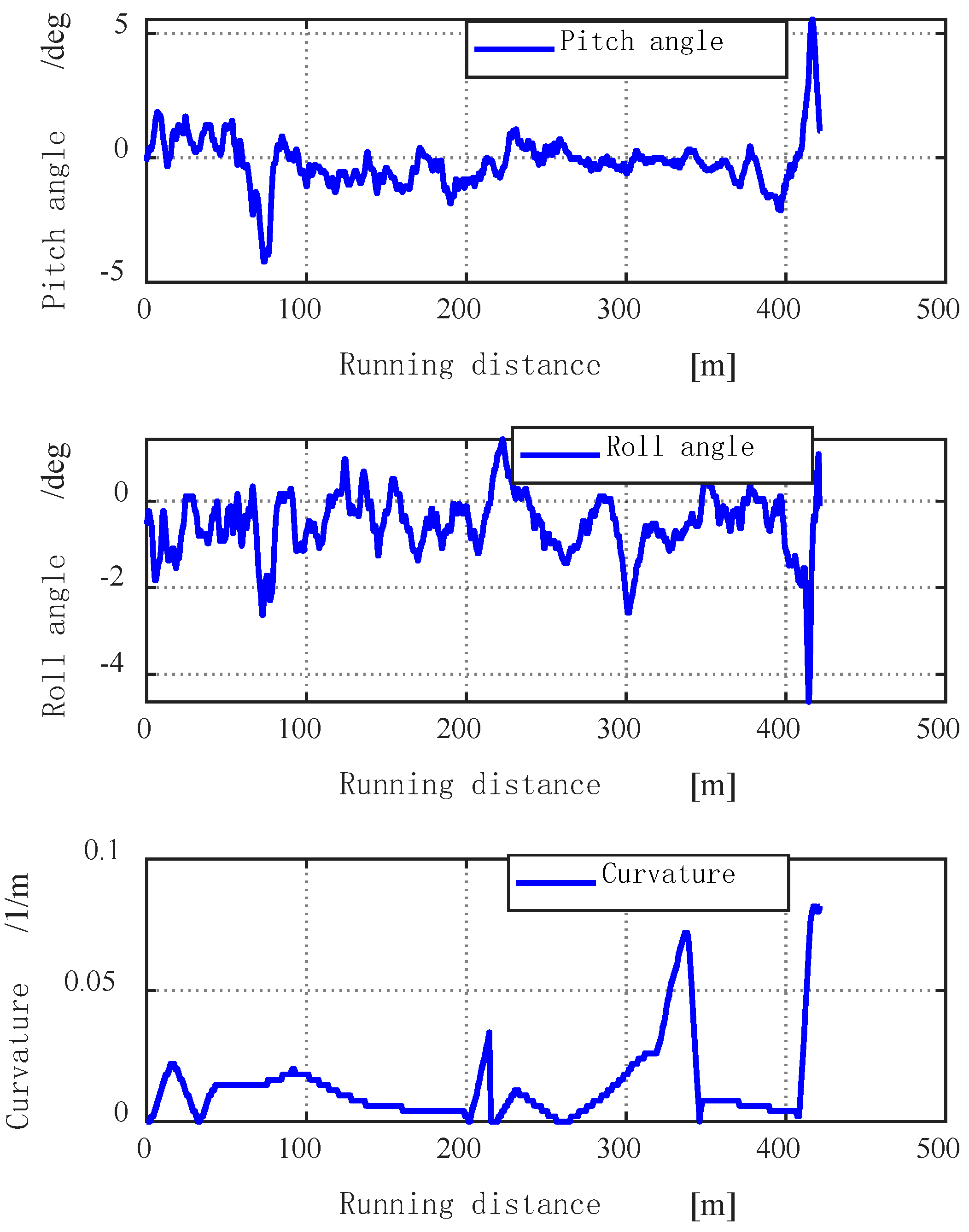
Figure 11. The vehicle uses the MPC controller and the Stanley controller to perform U-turn tests in a narrow area. Except for the lateral controller, the other configurations are the same. The vehicle inertial navigation acquires the pitch and roll angles. The turbulence of the line is evaluated by the pitch and roll angles, and the bending degree of the line is evaluated by the curvature of the line. The bumps and bends of the lines are shown in
Figure 12.
It can be seen from
Figure 12 that the pitch angle and the roll angle have great changes, reflecting that the road surface quality of the line is poor and very bumpy. The curvature of the line changes greatly and the maximum curvature is 0.082, indicating that the line has a large curvature at this time.
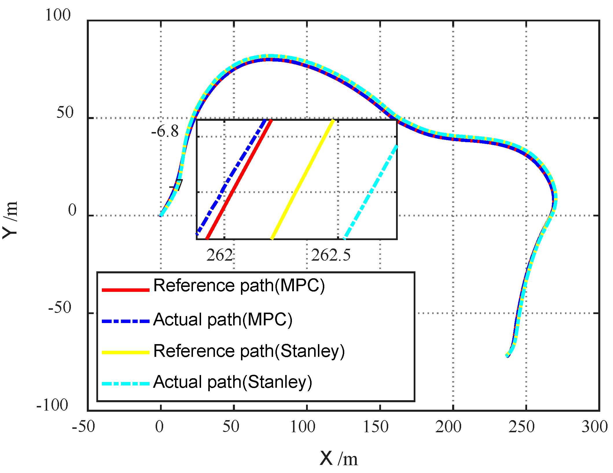
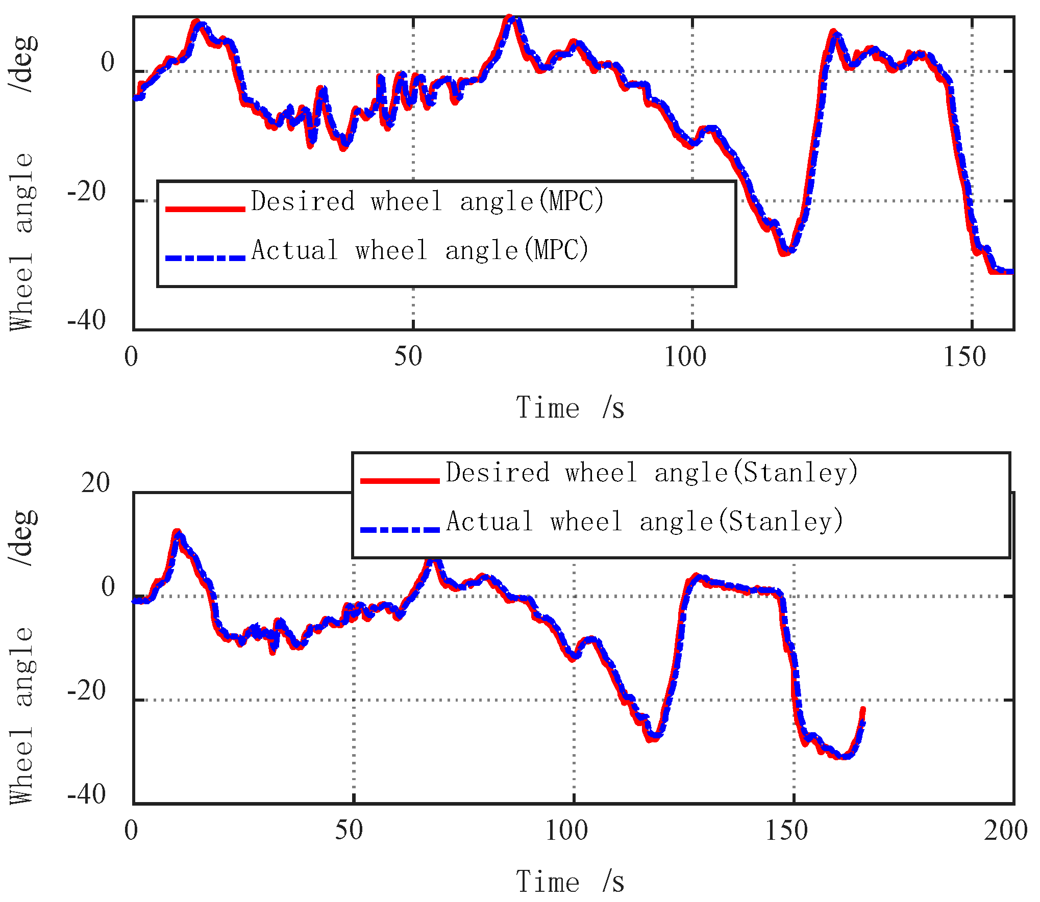
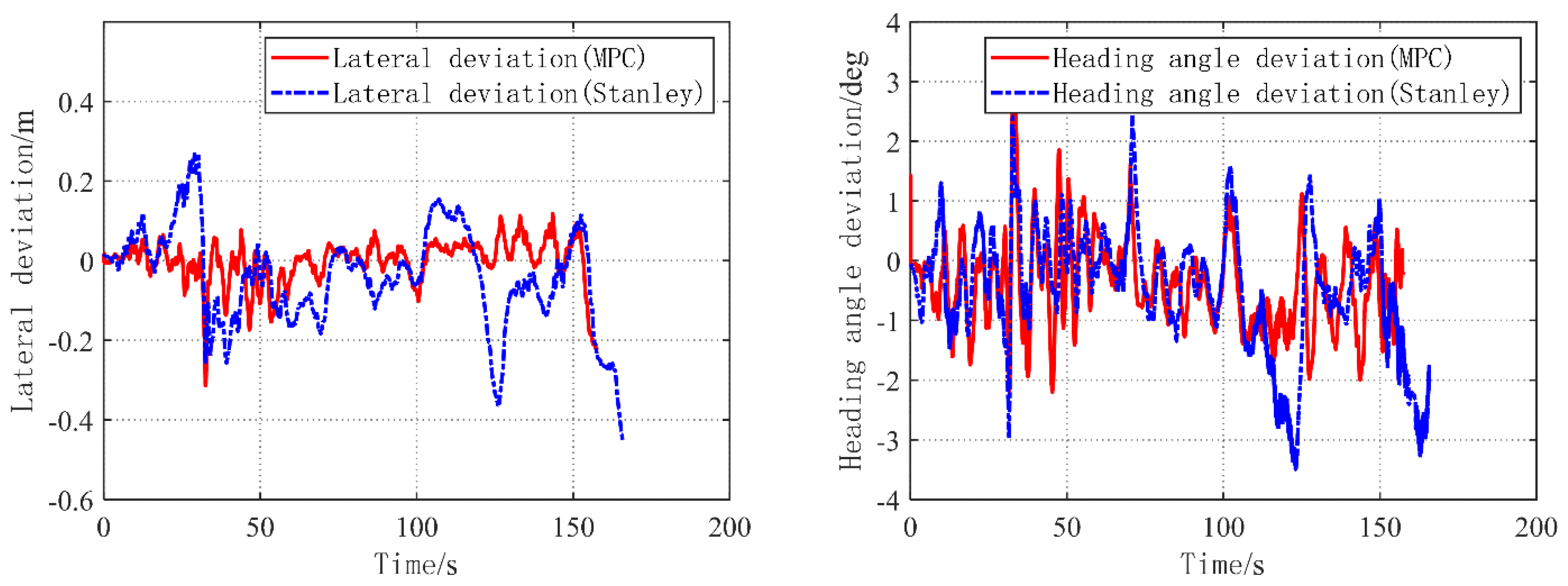
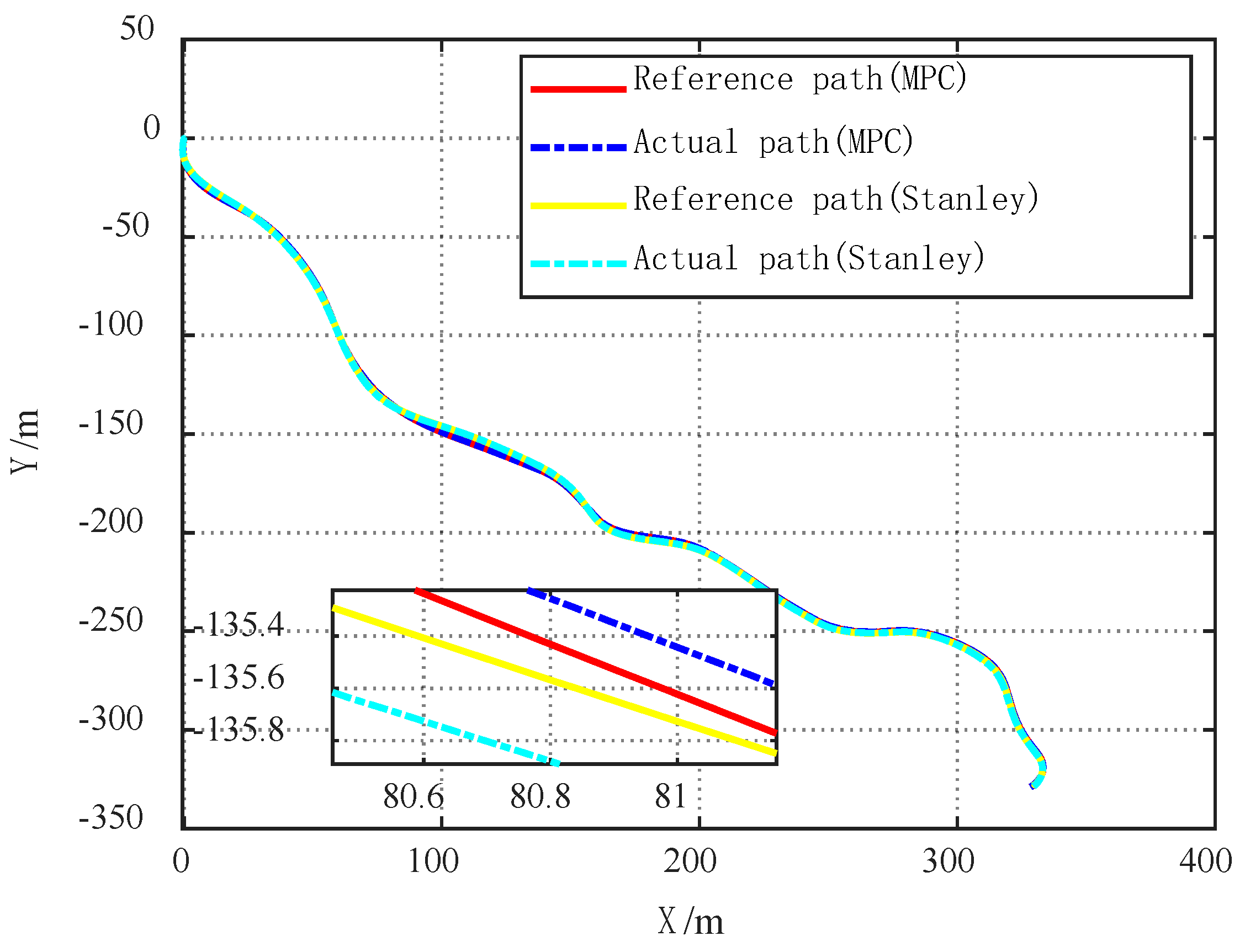
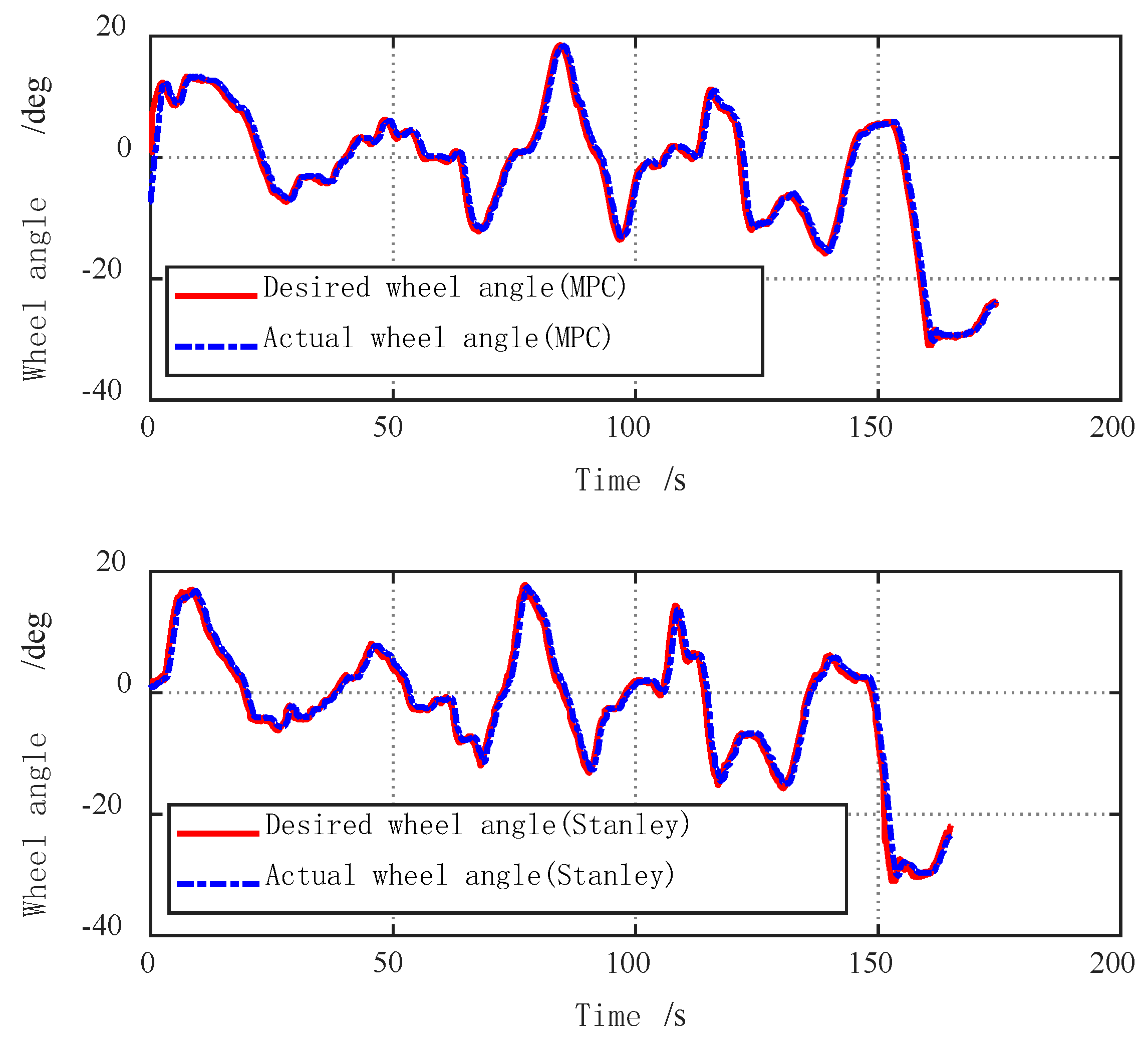
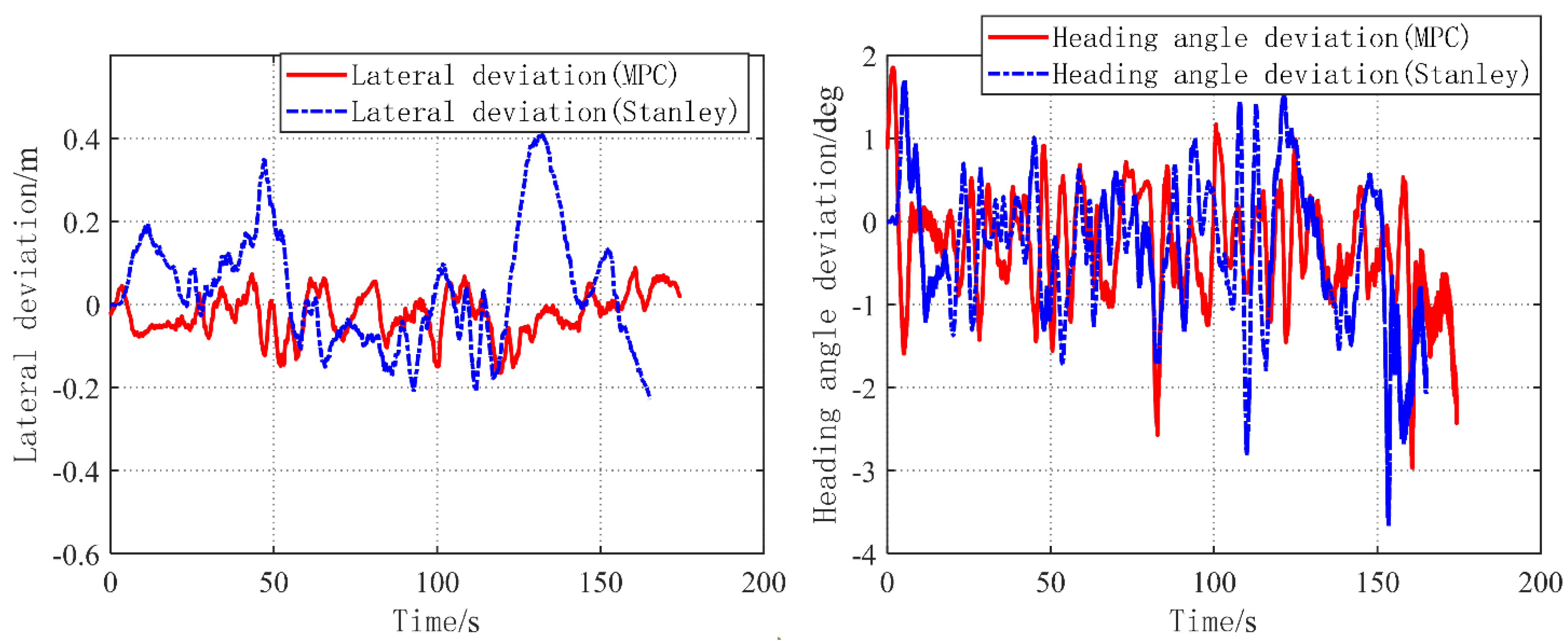
Under the S-shaped reference path with the target speed of 20 km/h, the vehicle is tested with the MPC controller and the Stanley controller, respectively. Except for the lateral controller, other configurations are the same. The experimental results are shown in
Figure 16,
Figure 17,
Figure 18.
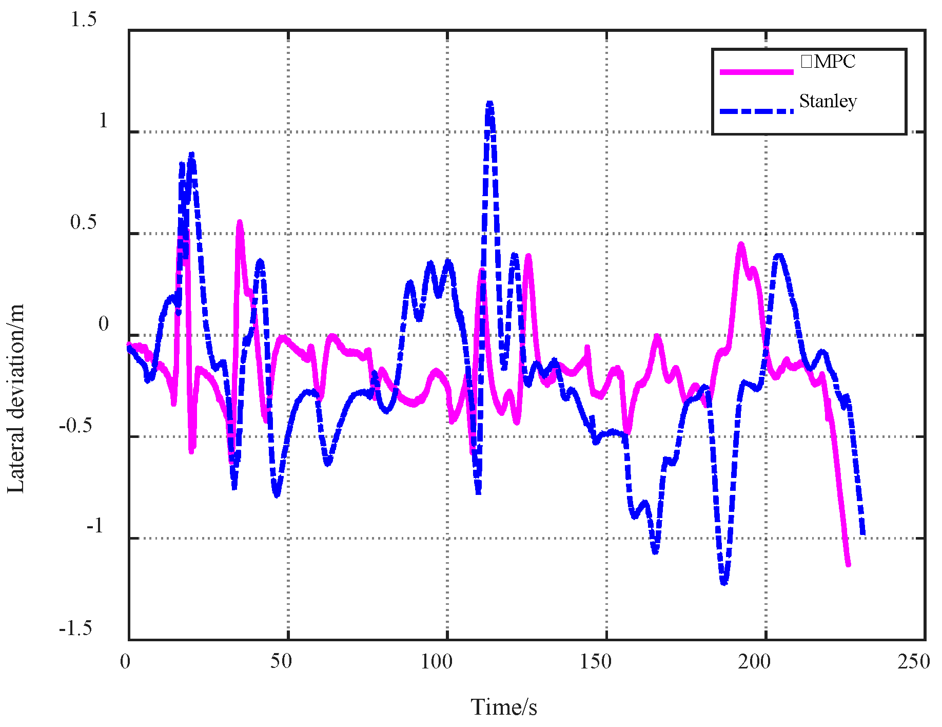
It can be seen from the above test results that under the complex working conditions of the “C” shape and “S” shape reference path, the MPC control algorithm has a significantly improved control effect on the lateral deviation than the Stanley algorithm, and the control effect on the heading angle deviation is comparable. Under the “C” shape reference path, the maximum lateral deviation is reduced from 0.55 m to 0.08 m, and the average lateral deviation is reduced from 0.19 m to 0.02 m, and under the “S” shape reference path, the maximum lateral deviation is reduced from 0.4 m to 0.16 m, the average lateral deviation was reduced from 0.12 m to 0.05 m.
7. Conclusions
In this paper, in the complex operating environment of open-pit mine transportation vehicles, caused by road bumps, large undulating ramps, and turns in narrow areas, as well as the large delay of vehicle steering actuators and poor response accuracy, the path tracking control has large tracking lateral deviation. For the problem of left and right fluctuations, a comparative study of some path control methods is first conducted. The conclusion is that the MPC method performs best in terms of tracking accuracy, and the actuator delay compensation can be explicitly considered. Then, based on the MPC method, the problem of unmanned path tracking control of open-pit mine transportation vehicles is mainly studied. Finally, it is verified by the real vehicle test that compared with the traditional method, the path tracking control method based on MPC can reduce the lateral control deviation from 0.55 m to 0.08 m under the C-shaped reference path, and from 0.4 m under the S-shaped reference path it was reduced to 0.16 m, while the heading angle deviation did not deteriorate, and there was an improvement trend. In the process of using the lateral MPC, the delay response characteristics of the steering actuator are considered, and the response delay model of the steering actuator is established and applied to the process of calculating the output of the desired wheel angle by the MPC, which improves the lateral control accuracy. The lateral MPC control strategy used on the minecart is also applicable to front-wheel-steered passenger cars.
The future work will combine the path planning to carry out the research on the integration of regulation and control, so that the path tracking control problem can be optimized in terms of lateral deviation and heading angle deviation at the same time, and the horizontal and vertical coupling dynamic control will be considered to further improve the control accuracy.
Author Contributions
Conceptualization, Z.L.; Methodology, Z.L. and X.M.; Software, X.Y.; Validation, Z.L. and C.H.; Writing—original draft preparation, Z.L. and X.M.; Writing—review and editing, Z.L. and X.Y.; Visualization, C.H. All authors have read and agreed to the published version of the manuscript.
Funding
This research received no external funding.
Institutional Review Board Statement
Not applicable.
Informed Consent Statement
Not applicable.
Data Availability Statement
Not applicable.
Conflicts of Interest
Zhiyong Lei, Xiaolong Ma are employees of National Energy Group Shanxi Shenyan Coal Co., Ltd. Xiwen Yuan, Chuan He are employees of CRRC Zhuzhou Institute Co., Ltd. The paper reflects the views of the scientists and not the company. The authors declare no conflict of interest.
References
- Lima, P.F.; Pereira, G.C.; Mårtensson, J.; Wahlberg, B. Experimental validation of model predictive control stability for autonomous driving. Control Eng. Pract. 2018, 81, 244–255. [Google Scholar] [CrossRef]
- Paden, B.; Čáp, M.; Yong, S.Z.; Yershov, D.; Frazzoli, E. A survey of motion planning and control techniques for self-driving urban vehicles. IEEE Trans. Intell. Veh. 2016, 1, 33–55. [Google Scholar] [CrossRef] [Green Version]
- Lu, X.; Ai, Y.; Tian, B. Real-time mine road boundary detection and tracking for autonomous truck. Sensors 2020, 20, 1121. [Google Scholar] [CrossRef] [PubMed] [Green Version]
- Pendleton, S.D.; Andersen, H.; Du, X.; Shen, X.; Meghjani, M.; Eng, Y.H.; Rus, D.; Ang, M.H., Jr. Perception, planning, control, and coordination for autonomous vehicles. Machines 2017, 5, 6. [Google Scholar] [CrossRef]
- Choi, J.M.; Liu, S.Y.; Hedrick, J.K. Human driver model and sliding mode control—Road tracking capability of the vehicle model. In Proceedings of the 2015 European Control Conference, Linz, Austria, 15–17 July 2015; IEEE: New York, NY, USA, 2015; pp. 2132–2137. [Google Scholar]
- Bai, G.; Liu, L.; Meng, Y.; Luo, W.; Gu, Q.; Ma, B. Path tracking of mining vehicles based on nonlinear model predictive control. Appl. Sci. 2019, 9, 1372. [Google Scholar] [CrossRef] [Green Version]
- Lima, P.F.; Nilsson, M.; Trincavelli, M.; Mårtensson, J.; Wahlberg, B. Spatial model predictive control for smooth and accurate steering of an autonomous truck. IEEE Trans. Intell. Veh. 2017, 2, 238–250. [Google Scholar] [CrossRef] [Green Version]
- Xu, S.; Peng, H.; Tang, Y. Preview path tracking control with delay compensation for autonomous vehicles. IEEE Trans. Intell. Trans. Syst. 2020, 22, 2979–2989. [Google Scholar] [CrossRef]
- Lima, P.F. Optimization-Based Motion Planning and Model Predictive Control for Autonomous Driving. Ph.D. Thesis, Royal Institute of Technology, Stockholm, Sweden, 2018. [Google Scholar]
- Li, M.; Imou, K.; Wakabayashi, K.; Yokoyama, S. Review of research on agricultural vehicle autonomous guidance. Int. J. Agric. Biol. Eng. 2009, 2, 1–16. [Google Scholar]
- Li, T.; Hu, J.; Gao, L.; Hu, H.; Bai, X.; Liu, X. Research on straight-line path tracking control methods in an agricultural vehicle navigation system. In Proceedings of the 11th International Conference on Precision Agriculture, Indianapolis, IN, USA, 15–18 July 2022. [Google Scholar]
- Thrun, S.; Montemerlo, M.; Dahlkamp, H.; Stavens, D.; Aron, A.; Diebel, J.; Fong, P.; Gale, J.; Halpenny, M.; Hoffmann, G.; et al. Stanley: The Robot that Won the DARPA Grand Challenge. J. Field Robot. 2006, 23, 661–692. [Google Scholar] [CrossRef]
- Hoffmann, G.M.; Tomlin, C.J.; Montemerlo, M.; Thrun, S. Autonomous automobile trajectory tracking for off-road driving: Controller design, experimental validation and racing. In Proceedings of the American Control Conference, New York, NY, USA, 9–13 July 2007; IEEE: New York, NY, USA, 2007; pp. 2296–2301. [Google Scholar]
- Raffo, G.V.; Gomes, G.K.; Normey-Rico, J.E.; Kelber, C.R.; Becker, L.B. A predictive controller for autonomous vehicle path tracking. IEEE Trans. Intell. Transp. Syst. 2009, 10, 92–102. [Google Scholar] [CrossRef]
- Nam, H.; Choi, W.; Ahn, C. Model predictive control for evasive steering of an autonomous vehicle. Int. J. Automot. Technol. 2019, 20, 1033–1042. [Google Scholar] [CrossRef]
- Kim, E.; Kim, J.; Sunwoo, M. Model predictive control strategy for smooth path tracking of autonomous vehicles with steering actuator dynamics. Int. J. Automot. Technol. 2014, 15, 1155–1164. [Google Scholar] [CrossRef]
- Falcone, P.; Borrelli, F.; Asgari, J.; Tseng, H.E.; Hrovat, D. Predictive Active Steering Control for Autonomous Vehicle Systems. IEEE Trans. Control Syst. Technol. 2007, 15, 566–580. [Google Scholar] [CrossRef]
- Hao, S.; Bu, D.; Du, Y.; Liu, H. Accelerated Solution Method for Vehicle Trajectory Tracking Based on Model Predictive Control. J. Hunan Univ. Nat. Sci. 2020, 47, 24–30. (In Chinese) [Google Scholar]
- Yakub, F.; Mori, Y. Comparative study of autonomous path-following vehicle control via model predictive control and linear quadratic control. Proc. Inst. Mech. Eng. D J. Aut. Eng. 2015, 229, 1695–1714. [Google Scholar] [CrossRef]
- Ye, H.; Jiang, H.; Ma, S.; Tang, B.; Wahab, L. Linear model predictive control of automatic parking path tracking with soft constraints. Int. J. Adv. Robot. Syst. 2019, 16, 1729881419852201. [Google Scholar] [CrossRef] [Green Version]
Figure 1.
Geometric analysis of pure pursuit method.
Figure 1.
Geometric analysis of pure pursuit method.
Figure 2.
Geometric analysis of Stanley method.
Figure 2.
Geometric analysis of Stanley method.
Figure 3.
MPC control block diagram based on delay model.
Figure 3.
MPC control block diagram based on delay model.
Figure 4.
Actuator step response curve (left). Comparison between actual steering curve and model calculation curve (right).
Figure 4.
Actuator step response curve (left). Comparison between actual steering curve and model calculation curve (right).
Figure 5.
Hardware-in-the-loop simulation platform (left). Virtual simulation map (right).
Figure 5.
Hardware-in-the-loop simulation platform (left). Virtual simulation map (right).
Figure 6.
Global trajectory of MPC control and Stanley control (left). Large curvature route (right).
Figure 6.
Global trajectory of MPC control and Stanley control (left). Large curvature route (right).
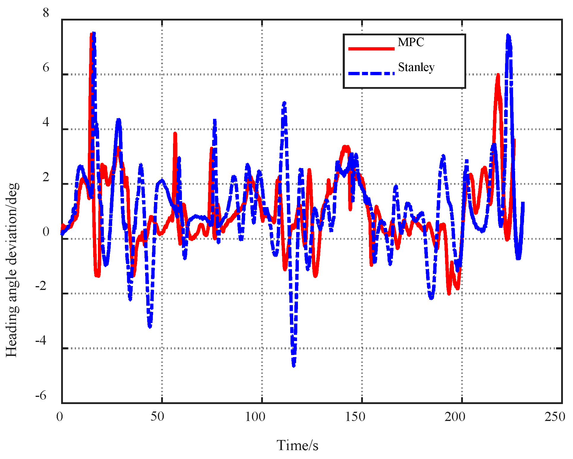
Figure 7.
Heading angel deviation of MPC control and Stanley control.
Figure 7.
Heading angel deviation of MPC control and Stanley control.
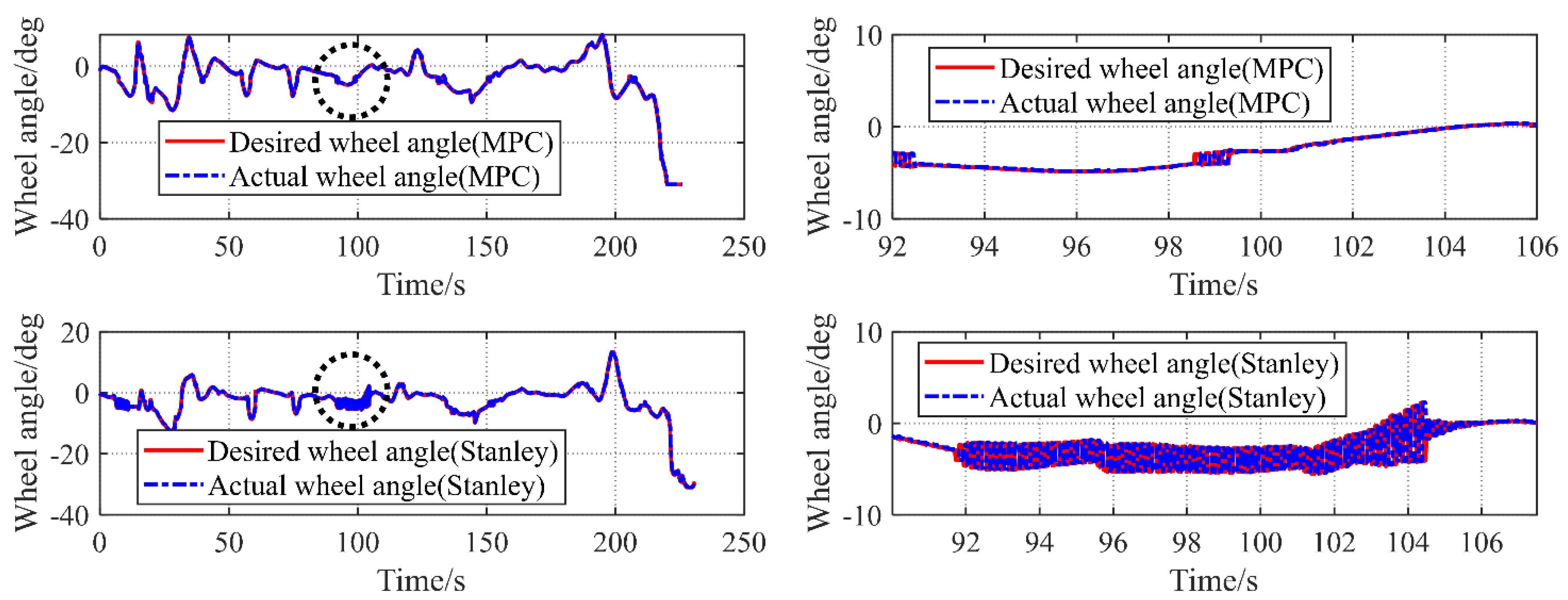
Figure 8.
Vehicle wheel angle of MPC control and Stanley control (left). Control stability comparison (right).
Figure 8.
Vehicle wheel angle of MPC control and Stanley control (left). Control stability comparison (right).
Figure 9.
Lateral deviation of MPC control and Stanley control.
Figure 9.
Lateral deviation of MPC control and Stanley control.
Figure 10.
Field test scenario: (a) mining truck, (b) loading job scenarios, (c) autonomous driving operation scenario, and (d) unloading job scenario.
Figure 10.
Field test scenario: (a) mining truck, (b) loading job scenarios, (c) autonomous driving operation scenario, and (d) unloading job scenario.
Figure 11.
Vehicle speed.
Figure 11.
Vehicle speed.
Figure 12.
Vehicle pitch angle and roll angle and route curvature.
Figure 12.
Vehicle pitch angle and roll angle and route curvature.
Figure 13.
Global trajectory of MPC control and Stanley control.
Figure 13.
Global trajectory of MPC control and Stanley control.
Figure 14.
Vehicle wheel angle of MPC control and Stanley control.
Figure 14.
Vehicle wheel angle of MPC control and Stanley control.
Figure 15.
Lateral error and heading angle deviation of MPC control and Stanley control.
Figure 15.
Lateral error and heading angle deviation of MPC control and Stanley control.
Figure 16.
Global trajectory of MPC control and Stanley control.
Figure 16.
Global trajectory of MPC control and Stanley control.
Figure 17.
Vehicle wheel angle of MPC control and Stanley control.
Figure 17.
Vehicle wheel angle of MPC control and Stanley control.
Figure 18.
Lateral error and heading angle deviation of MPC control and Stanley control.
Figure 18.
Lateral error and heading angle deviation of MPC control and Stanley control.
Table 1.
Lateral error test results.
Table 1.
Lateral error test results.
| Working Condition | Method | Maximum Deviation/m | Average Deviation/m |
|---|
Reference speed 30 km/h,
“C” shape reference path | MPC | 0.6 | 0.2 |
| Stanley | 1.2 | 0.6 |
Table 2.
Controller parameters.
Table 2.
Controller parameters.
| Parameters | MPC |
|---|
| Prediction horizon Np | 80 |
| Control horizon Nc | 80 |
| Discrete step size T/s | 0.1 |
| Control frequency f/Hz | 50 |
| Weight coefficient matrix Q | diag(100, 1) |
| Weight coefficient R | 1 |
Table 3.
Lateral error test results.
Table 3.
Lateral error test results.
| Scenarios | Method | Maximum Deviation/m | Average Deviation/m |
|---|
Speed target 10 km/h,
“C” shape reference path | MPC | 0.08 | 0.02 |
| Stanley | 0.55 | 0.19 |
Speed target 20 km/h,
“S” shape reference path | MPC | 0.16 | 0.05 |
| Stanley | 0.40 | 0.12 |
| Publisher’s Note: MDPI stays neutral with regard to jurisdictional claims in published maps and institutional affiliations. |
© 2022 by the authors. Licensee MDPI, Basel, Switzerland. This article is an open access article distributed under the terms and conditions of the Creative Commons Attribution (CC BY) license (https://creativecommons.org/licenses/by/4.0/).


