Article

Map Construction Based on LiDAR Vision Inertial Multi-Sensor Fusion

College of Mechanical Engineering, Xi’an University of Science and Technology, Xi’an 710054, China
*
Author to whom correspondence should be addressed.
World Electr. Veh. J. 2021, 12(4), 261; https://doi.org/10.3390/wevj12040261
Submission received: 11 November 2021 / Revised: 5 December 2021 / Accepted: 10 December 2021 / Published: 12 December 2021

Abstract

:
In order to make up for the shortcomings of independent sensors and provide more reliable estimation, a multi-sensor fusion framework for simultaneous localization and mapping is proposed in this paper. Firstly, the light detection and ranging (LiDAR) point cloud is screened in the front-end processing to eliminate abnormal points and improve the positioning and mapping accuracy. Secondly, for the problem of false detection when the LiDAR is surrounded by repeated structures, the intensity value of the laser point cloud is used as the screening condition to screen out robust visual features with high distance confidence, for the purpose of softening. Then, the initial factor, registration factor, inertial measurement units (IMU) factor and loop factor are inserted into the factor graph. A factor graph optimization algorithm based on a Bayesian tree is used for incremental optimization estimation to realize the data fusion. The algorithm was tested in campus and real road environments. The experimental results show that the proposed algorithm can realize state estimation and map construction with high accuracy and strong robustness.

1. Introduction

At present, the simultaneous localization and mapping (SLAM) algorithm plays an important role in mobile robot navigation. The mainstream SLAM technologies fall into two categories: laser and vision SLAM. The laser-based SLAM has some advantages, such as its high resolution, strong anti-interference ability and accurate obstacle distance information. However, LiDAR is vulnerable to the corridor effect in unstructured environments because it is difficult to provide reliable motion estimation. Therefore, in the process of building a point cloud map, motion distortion will be caused by receiving distance measurements data at different times. Although vision-based SLAM has rich image feature information and a low repeatability of spatial features, meaning that the map has better global positioning, the positioning accuracy will be reduced because the image sensor is easily affected by the light, and there are few texture features in the environment. For the problem mentioned above, the mobile robot estimates its position information by wheel odometry and inertial measurement units (IMU), which improve the robustness and stability of the system. For the realization of accurate positioning and navigation, as well as the avoidance of the influence of environmental light changes and rapid scene movement, a multi-sensor fusion scheme has become the main research direction of SLAM technology.
In this paper, the feature extraction method in LiDAR front-end processing is mainly inspired by lightweight and ground-optimized LiDAR odometry and mapping (LEGO-LOAM). It divides the point cloud of LiDAR into ground points and segmentation points. Then, it divides the points into edge points and flat points according to smoothness. In this way, the efficiency and accuracy of the drawing construction can be improved. However, because LEGO-LOAM uses a rotating LiDAR velodyne, the number of point clouds is much smaller than the solid-state LIVOX used in this paper. We therefore screen the point clouds to eliminate unqualified points before extracting the LiDAR feature points, which effectively reduces the loss of computing resources. Note that LEGO-LOAM is a loosely-coupled system, and IMU measurements are not used in the optimization steps. In this paper, the IMU factor is imported into the factor graph for global optimization. Visual-LiDAR odometry and mapping (VLOAM) integrates the monocular camera and LiDAR information to build graphs, but does not add closed-loop detection. In this paper, closed-loop detection is set to periodically eliminate the drift caused by the robot.
This paper proposes a multi-sensor coupled SLAM framework which has four modules, as shown in Figure 1. The front-end module obtains images and laser point clouds from the camera and LiDAR, respectively. For the image data, feature point matching is obtained by feature point extraction and feature point tracking between two adjacent frames. For the LiDAR data, we filter and eliminate the noise point cloud, and then extract and match the features of the laser point cloud. The vision inertial LiDAR odometry module uses the visual features to compensate the LiDAR features, increasing the number of LiDAR feature points, in order to improve the mapping and positioning accuracy. In the pose estimation, the feature points of successive key frames are aligned and registered. Then, the map building module performs point cloud registration and a map update to build a large-scale high-precision map. The closed-loop detection module detects whether the trajectory is closed. As a closure factor, the pose relation of the closed position will be improved into the factor graph. Finally, the initial factor, registration factor, IMU factor and closed-loop factor are inserted into the factor graph for optimization. The motion trajectory can be obtained after incremental smoothing. The main contributions of this paper are as follows:
(1)
Before the LiDAR feature extraction, the point clouds are screened to eliminate the points that do not meet the conditions, so as to effectively reduce the loss of computing resources.
(2)
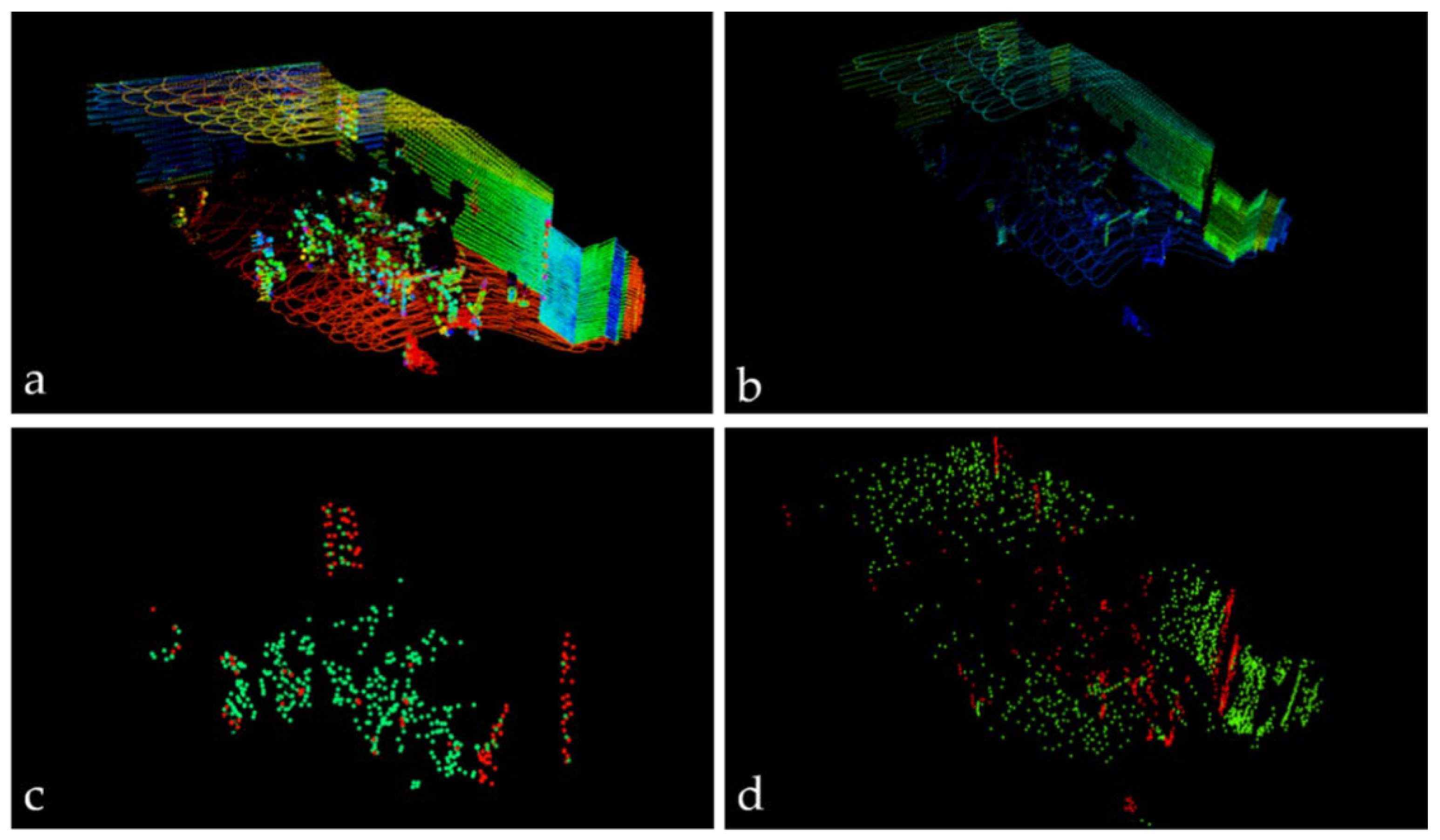
The visual features filtered through the intensity value of the point clouds are used to supplement the laser point cloud features, improving the accuracy of positioning and mapping.
(3)
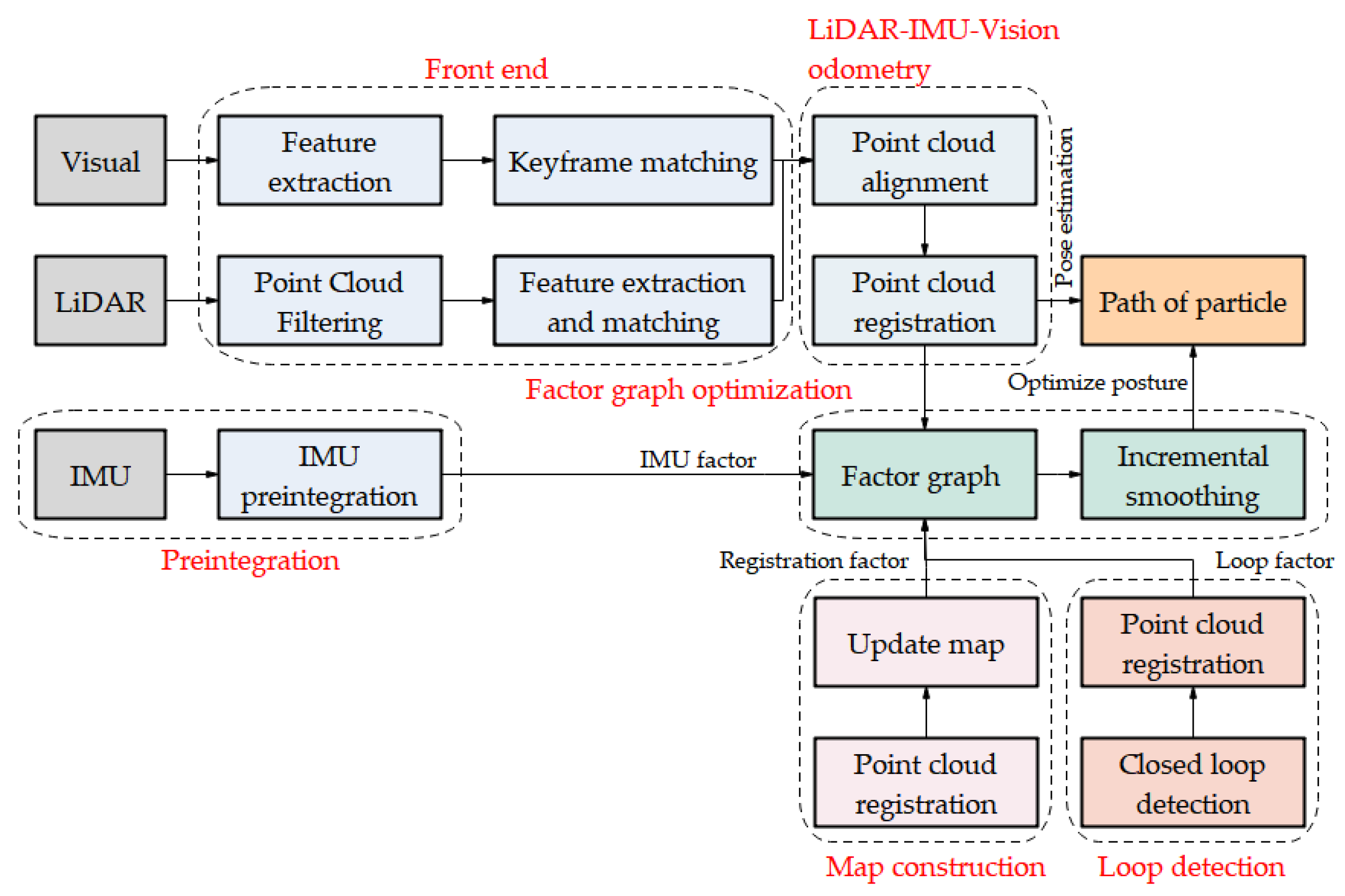
A close-coupled LiDAR vision inertial system based on factor graph optimization is proposed in order to realize multi-sensor information fusion and construct a three-dimensional point cloud map with high robustness in real-time.
The rest of the paper is organized as follows. First, Section 2 discusses previous work. Secondly, Section 3 describes the details, state estimation based on factor graph optimization, front-end processing of the vision and LiDAR, IMU pre-integration, odometry of fusion vision IMU LiDAR, map construction, closed-loop detection and factor graph optimization. Then, Section 4 presents the experimental verifications. Finally, Section 5 summarizes the full text.

2. Previous Work

Zhao [1] used the feature parameterization of the Fourier series to optimize the irregular closed features, and reduced the time dependency of the initial guess through a subgraph connection. Mur-Artal et al. proposed a monocular SLAM method based on oriented fast and rotated brief (ORB) features [2], ORB-SLAM [3], which can realize the real-time positioning of indoor and outdoor environments by monocular cameras, and can generate a compact traceable map. In order to solve the problem that monocular cameras can’t restore the realistic scale, Mur-Artal et al. came up with an approach called ORB-SLAM2 [4], which added binocular cameras and red-green-blue-depth (RGB-D) cameras to estimate the depth. Vladyslav et al. put forward the system called binocular vision inertial odometry direct visual-inertial (DVIO) [5], which estimates the attitude, speed and IMU noise of the camera by minimizing the photometric error, as well as taking the minimization of the energy function as the optimization goal. This method is not only better than the algorithm relying only on vision or loose coupling but also has high accuracy under rapid motion and significant illumination changes. Qin et al. proposed the tightly coupled SLAM system [6], which is a sliding window based on visual inertia. This approach is a multi-sensor state estimator based on nonlinear optimization, supporting the data fusion of multiple visual inertial sensors and realizing high-precision autonomous positioning. Campos et al. extended ORB-SLAM2 by fusing camera and IMU measurement. As a result, ORB-SLAM3 [7] was created. However, the cost of high-end IMU is very high, while low-precision IMU is vulnerable to Gaussian white noise and drift. Qin et al. came up with a powerful monocular vision inertial state estimator versatile monocular visual-inertial system monocular (VINS-MONO) [8]. This system uses a local nonlinear optimization algorithm based on a sliding window to keep the computational complexity constant by constraining the number of key frames in the sliding window. At the same time, it can also estimate the monocular scale factor, IMU bias and external parameters between IMU and the camera in real time. Therefore, this system has very good robustness.
The fusion of LiDAR inertial odometry (LIO) is usually divided into loose coupling and tight coupling. Loosely-coupled LIO methods typically process the LiDAR and IMU measurements separately and fuse their results later. The 3D laser LiDAR odometry and mapping (LOAM) [9] proposed by Zhang and the LEGO-LOAM [10] based on ground optimization proposed by Shan et al. are loosely coupled methods. LOAM takes the pose integrated from IMU measurements as the initial estimate for the LiDAR scan registration. However, LOAM directly stores the global voxel map rather than the local map, making it difficult to perform closed-loop detection to correct the drift. A common procedure in the loosely-coupled approach is to obtain a pose measurement by registering a new scan and then fusing the pose measurement with the IMU measurements. The separation between scan registration and data fusion reduces the computation load. However, it ignores the correlation between the system’s other states and the pose of the new scan. Moreover, in the case of featureless environments, the scan registration could degenerate in certain directions, and causes unreliable fusion in later stages. The difference between our work and the above is that LOAM directly stores the global voxel map, which makes it impossible for closed-loop detection to correct the cumulative error. This article uses incremental map construction to compare the current point cloud scan with the constructed global map. The point clouds are superimposed together to eliminate the cumulative error caused by the pose estimation. Unlike the loosely-coupled method, the tightly-coupled LiDAR-inertial odometry methods typically fuse the raw feature points of LiDAR with IMU data. There are two main approaches to tightly-coupled LIO: optimization-based and filter-based. LIO-SAM [11] obtains the globally consistent pose of the robot through factor graph optimization. This method uses frame and local map matching instead of LOAM frame and global map matching, which improves the matching efficiency. LIO-Mapping [12] embeds a rotation-constrained thinning algorithm to further align the LiDAR attitude with the global map, but the optimization of all of the measured values can’t ensure real-time performance. Zhao [13] proposed the LIOM package, which uses a similar graph optimization but based on edge and plane features. Geneva [14] used graph optimization with IMU pre-integration constraints and plane constraints from LiDAR feature points. For filter-based methods, Bry [15] used a Gaussian Particle Filter (GPF) to fuse the data of IMU and a planar 2D LiDAR. This method was also used in the Boston Dynamics Atlas humanoid robot.
Recently, LiDAR-visual-inertial systems have attracted increased attention due to their robustness in sensor-degraded tasks [16]. J Zhang et al. raised VLOAM [17], which loosely integrates monocular cameras and LiDAR. Similarly to LOAM, it does not add closed-loop detection. SEO [18] established LiDAR and visual maps in parallel, and used odometry residuals to maintain the global consistency between LiDAR voxel maps and operating environments. Through this close-coupling method, odometry can be estimated more accurately. Jiang et al. [19] developed a cost function execution graph optimization considering LiDAR data and image data, and constructed a 2.5D map to accelerate cycle detection. Lin et al. designed the system LOAM-LIVOX [20]. Through processing on the front and back ends of SLAM, they solved some challenges brought by this non-repetitive scanning LiDAR. High accuracy can be achieved at low speeds, while pose estimation will drift greatly in high-speed operation. In order to improve the loop detection and graphics optimization performance of point cloud matching, Chen [21] built a LiDAR and vision fusion SLAM backend, using the geometric and visual features of the LiDAR to complete loop detection, and re-matching the point cloud to verify closed loop detection and complete the graph optimization. Wang [22] proposed direct visual LiDAR odometry and mapping, which is the first framework that combines a depth-enhanced direct visual odometry module and the LiDAR mapping module into location and mapping. It takes advantage of the efficiency of the direct visual odometry module and the accuracy of the LiDAR scan-to-map matching method.

3. Methods

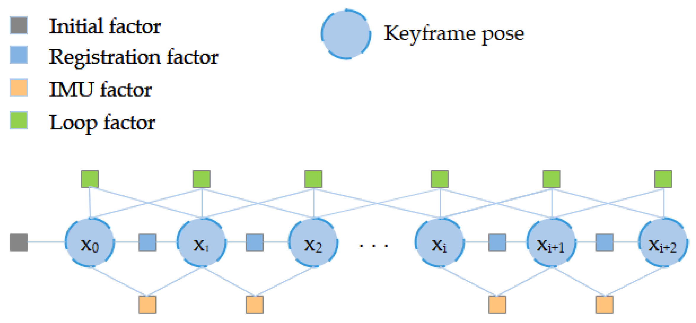
3.1. State Estimation Based on Factor Graph Optimization

The world coordinate system is represented as W , and the carrier coordinate system is represented as B . Suppose that the starting time of the LiDAR’s i-th scan is t i , scanned point clouds are marked as i , and the data collected by IMU in [ t i , t j ] is recorded as ( i , j ) ; the motion state of the system x i can be expressed as
x i = [ R i T , P i T , V i T , b i T ] T
where the rotation matrix is R S O ( 3 ) , the position vector is P 3 , the velocity vector is V 3 and zero bias is b . b is determined by gyro zero bias b g and accelerometer zero bias b a .
The rigid body transformation from the carrier coordinate system B to the world coordinate system W is carried out under T = [ R | p ] S E ( 3 ) . In order to reduce the computational complexity, the key frame is selected as the state quantity of the optimization estimation. Define K k is all keyframes at time t k ; the corresponding state quantity is X k = { x i } i K k , and the observation is Z k = { i , ( i , j ) } ( i , j ) K k . The state estimation problem can be expressed as the maximum a posteriori problem. Given the observation information and the prior information, estimate the posterior probability of X k :
p ( X k | Z k ) p ( X 0 ) p ( Z k | X k ) = p ( X 0 ) ( i , j ) K k ( i , ( i , j ) | X k ) = p ( X 0 ) ( i , j ) K k ( ( i , j ) | x i , x j ) i K k p ( i | x i )
The maximum a posteriori probability of the variable factor can be derived from Equation (2):
X k ^ = argmin X k ( ln p ( X k | Z k ) ) = argmin X k ( 𝓇 0 Σ 0 2 + ( i , j ) K k 𝓇 ( i , j ) Σ ( i , j ) 2 + i K k 𝓇 Σ i 2 + i K k 𝓇 ( i , j ) Σ ( i , j ) 2 )
where 𝓇 0 , 𝓇 ( i , j ) ,   𝓇 i ,   𝓇 ( i , j ) represents the residual associated with the measured value. Σ 0 , Σ ( i , j ) , Σ i , Σ ( i , j ) is the corresponding covariance matrix, and the items in Equation (3) will be described in detail later.

3.2. Vision and LiDAR Front End

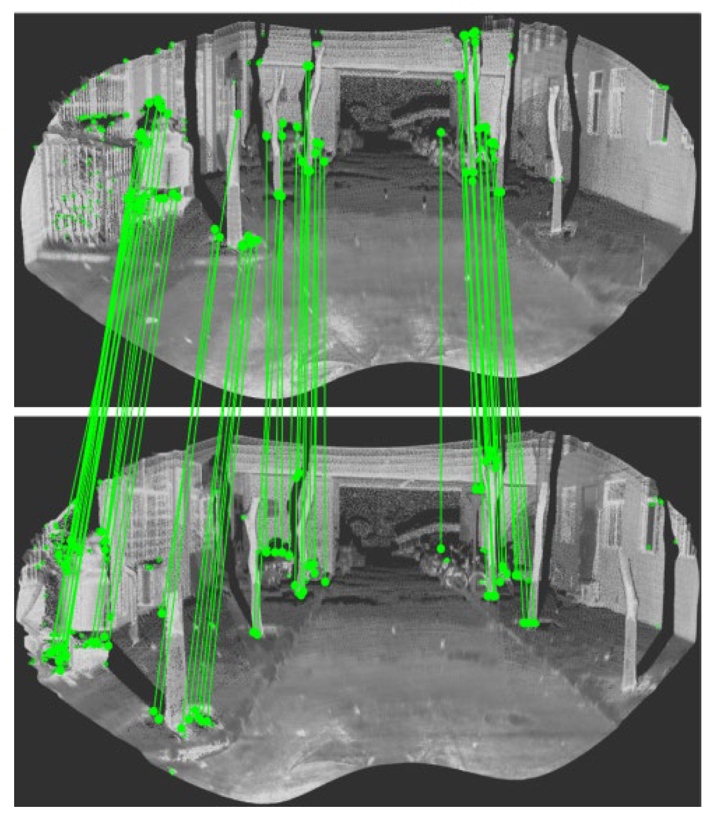
3.2.1. Visual Front End

The visual feature points used in this article are ORB feature points, which are composed of two parts: an improved FAST corner point and a BRIEF [23] descriptor. The improved FAST corner points are used to extract pixels with obvious differences in the image. The gray-scale centroid algorithm is added to improve the rotation invariance of the feature points. In addition, the characteristics of the pixels are judged by the BRIEF descriptor to determine the position of the ORB feature points in the image. The principle of FAST corner detection is that if there are enough pixels on the neighborhood circle at a certain point, the gray value of which is quite different from the gray value of the center point of the neighborhood circle, the point may be a key point. Select a certain pixel p in the image as the center, set its brightness value as I p and the threshold T as 20% of the brightness value I p . Select 16 pixel points on a circle with radius 3 if there are 12 consecutive pixels on the circle. If the brightness value of the point is outside the range   ( I p T , I p + T ) , then this pixel point p can be used as a feature point. The number of corner points extracted by FAST is too large and not very stable. This article specifies the number of corner points to be extracted N. By calculating the Harris response value of the corner points, the response values are arranged from large to small, and the first N is selected. One corner point with the largest response value is used as the final feature point to be extracted in order to eliminate the problem of excessive corner points and instability. In addition, the corner points extracted by FAST do not have scale information and lack directionality. This article constructs an image pyramid. The bottom layer of the pyramid is the original image. For each upper layer, the image is down-sampled with a scaling factor of 1.2 to obtain a total of 8 images. In feature matching, the scale invariance is achieved by matching images on different layers. Calculate the gray centroid in the neighborhood S of the feature point and use it as the end of the vector. The direction of the vector is used as the direction of the feature point. The gray moment of the neighborhood S of the feature point is defined as follows:
m p q = x , y B x p y q I ( x , y )
where x and y are the coordinates of the pixel, and I ( x , y ) is the gray value of the pixel.
Then, the gray-scale centroid C of the image and the dominant direction θ of the feature point can be obtained by using the gray-scale moment of the image as follows:
C = ( m 10 m 00 , m 01 m 00 )
θ = a r c t a n ( m 01 m 10 )
The FAST feature point does not have the defect of directionality through the improvement of the gray centroid. After extracting the key points, use the BRIEF descriptor to describe the environmental information around the key points, which is a binary descriptor. This description method does not have rotation invariance. It is necessary to add the key point direction in the improved FAST to obtain the rotation characteristics of the descriptor. Then, rotate the image to the dominant direction of the feature point in order to calculate the BRIEF descriptor to obtain the rotation invariance. Finally, using the previous image frame as the initial posture, the optical flow method is used to continuously track the new image frame. Moreover, the rigid body transformation relationship between two adjacent key frames is estimated.

3.2.2. LiDAR Front End

By calculating the characteristics of each 3D point cloud F ( x , y , z ) , depth D is the distance to each point measured by LiDAR:
D ( F ) = x 2 + y 2 + z 2
Laser deflection Angle φ is the angle between the x axis and laser ray:
ϕ ( F ) = t a n 1 y 2 + z 2 x 2
The reflection intensity of LiDAR I ( F ) is:
I ( F ) = R / D ( F ) 2
where R is the reflectivity of the object measured by LiDAR. The reflection intensity I ( F ) is smaller, which indicates that the point is far away from the LiDAR sensor or the object’s reflectivity R is low.
(1)
In order to improve the accuracy of the positioning and mapping, the point cloud scanned by LiDAR is processed, and the irrelevant point clouds are eliminated by the following rules.
The points at the edge of the LiDAR angle of view are eliminated.
(2)
Eliminate the points with particularly large or small reflection intensities. Excessive intensity will lead to the saturation or distortion of the receiving circuit, and a too-small intensity will lead to the reduction of the signal-to-noise ratio, both of which will reduce the ranging accuracy.
(3)
Eliminate the points hidden behind the object, otherwise it will lead to the wrong edge features.
The remaining points are collectively referred to as candidate points. The candidate point cloud is projected into the distance image to judge the vertical dimension characteristics of the pixel points and whether they belong to the ground laser scanning range. The original point cloud scanned by LiDAR is shown in Figure 2a. According to this, the point cloud can be divided into ground points and split points, as shown in Figure 2b. When the point cloud is projected into the image, the distance r from the pixel to the sensor can be calculated as r i . At the same time, the continuous point set in the distance image is collectively referred to as S . Calculate the smoothness c of each point in the point set, and set the threshold c th to distinguish the characteristics of the points. Those with a smoothness greater than the threshold are edge points; otherwise, they are plane points. In order to evenly extract features from all directions, the LiDAR scanning data is divided into two subsets in the horizontal direction. The smoothness of the points in the subset is sorted, and the edge feature point i e with the largest roughness and not belonging to the ground is selected from each row of the subset. Then, mark the plane feature point i f with the minimum roughness as a ground or segment point in the same way, as shown in Figure 2c.
c = 1 | S | r i j S , j i ( r j r i )
In order to create the point cloud images scanned by adjacent LiDAR through the sliding window method, n latest sub key frames { K i n , , K i } are extracted for the estimation, and the sub keyframe transformed by { T i n , , T i } is merged into a voxel map M i medium. M i e and M i f are the set of all of the edge and plane features in this process, and feature point set i e and i f are shown in Figure 2d.

3.3. IMU Pre-Integration

The observation model of IMU is
a ^ ( t ) = a ( t ) + b a ( t ) + R WB ( t ) g w + η a
ω ^ ( t ) = ω ( t ) + b g ( t ) + η ω
where η a , η ω represents observation noise, R WB represents the rotation matrix from B to W , and g w represents the gravitational acceleration in the world coordinate system. The presence of noise and deviation will affect the final measured value. Assuming that noise η a and η ω obey Gaussian distribution, acceleration offset b a and gyro offset b g are modeled as a random walk:
b ˙ a = n b a , b ˙ g = n b g
where n b a and n b g are subject to Gaussian distribution, and the corresponding moments of two consecutive key frames K i and K j are respectively b i and b j . From the state quantity at moment b i to the state quantity at moment b j , displacement P and velocity V can be obtained; the movement model of quaternion q is as follows:
P b j w = P b i w + V b i w Δ t + 1 2 t [ b i , b j ] R t w ( a ^ b a t ) g w dt 2 V b j w = V b i w + t [ b i , b j ] R t w ( a ^ b a t ) g w dt q b j w = q b i w t [ b i , b j ] 1 2 Ω ( ω ^ b w t ) q t b i dt
where P b j w is the pose of IMU in the world coordinate system at b j , V b j w is the velocity of IMU in the world coordinate system at b j , and q b j w is the quaternion of IMU in the world coordinate system at b j . If we multiply both sides of the three equations of (14) by R w b i , the integral part depends only on the measurement of IMU.
R w b i P b j w = R w b i ( P b i w + V b i w Δ t 1 2 g w Δ t 2 ) + α b j b i R w b i V b j w = R w b i ( V b i w g w Δ t ) + β b j b i q w b i q b j w = γ b j b i
where α b j b i is the position, β b j b i is the speed and γ b i b i 1 is the rotation. All can be propagated according to the measured values of IMU during the [ b i , b j ] time interval as follows:
α b j b i   t [ t i , t j ] R t b i ( a ^ b a t ) dt 2 β b j b i   t [ t i , t j ] R t b i ( a ^ b a t ) dt γ b j b i   t [ t i , t j ] 1 2 Ω ( ω ^ b w t ) γ t i b dt
where
Ω ( ω ) = { [ ω ] × ω ω T 0 } , [ ω ] × = { 0 ω z ω y ω z 0 ω x ω y ω x 0 }
Using the associated covariance estimation ^ s , j of the prior state s i , acceleration   a i and angular velocity ω i , the pose, speed and deviation of the next frame can be predicted. Therefore, the error equation of IMU is shown in Equation (17).
s ^ j h ( α b j b i ,   β b j b i , ε j , a i , ω i )
The IMU deviation term ε j 6 is used to measure the 3-axis acceleration and 3-axis angular velocity of IMU. Finally, the error equation of IMU is:
𝓇 ( i , j ) [ α b j b i α b j b i β b j b i + β b j b i ε + ε j ] T     ^ s , j 1 ( [ α b j b i α b j b i 1 β b j b i β b j b i ε ε j ] )

3.4. LiDAR-IMU-Vision Odometry

LiDAR has a long detection distance and a wider radiation range, and can capture many structural details in the environment. However, such details are often discarded during descriptor extraction, which may lead to false positive detections when surrounded by repetitive structures. At the same time, during the LiDAR measurement process, the ranging error on objects with a high reflection intensity is large, which is not conducive to the fusion of vision and LiDAR features. In this paper, the extracted visual feature points are used as the feature compensation points of LiDAR to eliminate the influence of repeated structure and ranging errors on LiDAR. Using solid-state LiDAR to provide a more dense point cloud, through the external parameter calibration of LiDAR and the vision sensor, we can obtain the rotation matrix R and the translation matrix T. What is more, the conversion relationship of points in different coordinate systems can be obtained. For example, any point collected by LiDAR is represented by F L ( x , y , z ) , and the image data collected by the camera is represented by F I m g ( u , v ) . Through the internal parameter matrix and the external parameter matrix, the point F L ( x , y , z ) is mapped to the point F I m g ( u , v ) :
( u v 1 ) = 1 Z C ( f u 0 u 0 0 f v v 0 0 0 1 ) [ ( R T 0 1 ) ( x y z 1 ) ] 3 × 3 = 1 Z C × K × [ E × ( x y z 1 ) ] 3 × 3
where Z C is the Z-axis value of the point in the camera coordinate system, K is the internal parameter matrix of the camera, and E is the external parameter matrix of the LiDAR and the camera.
According to formula (19), it can be shown that all points in the LiDAR coordinate system have one-to-one corresponding pixel points. Through the LiDAR front-end processing, we can calculate the reflection intensity I ( F L ) of F L at any point, so that we equivalently obtain the reflection intensity I ( F I m g ) of F I m g . Through feature extraction on the intensity image of the point cloud, according to the set laser reflection intensity range, the visual feature points with robustness and high distance confidence are selected. The total number of visual features screened is recorded as B . As the feature points in i e and i f are associated with each pixel in the intensity image, the LiDAR feature points are also associated with the visual feature points in B . The final fusion result is shown in Figure 3.
Convert the newly obtained LiDAR frame { i + 1 e , i + 1 f } from the B coordinate system to the W coordinate system, then obtain { i + 1 e , i + 1 f } . This initial transformation is obtained by using the robot motion predicted by IMU. For every feature of i + 1 e and i + 1 f , find its edge or plane correspondence in M i e or M i f . The matching point of   B i + 1 F j   i + 1 e consists of the nearest point   B i F k   i e and the sub adjacent point   B i F l   i f ; it can be obtained by a KD tree search. The distance d E from point   B i + 1 F j   to line {   B i F k   ,   B i F l   } is as follows:
d E = (   B i + 1 F j     B i F k   ) × (   B i + 1 F j     B i F l   )   B i F k     B i F l  
The matching point of   B i + 1 F j   i + 1 f consists of   B i F l   i f and   B i F m   i p , and the distance d F from point   B i + 1 F j   to plane {   B i F k   ,   B i F l   ,   B i F m   } is as follows:
d F = (   B i + 1 F j     B i F k   ) ( (   B i F k     B i F l   ) × (   B i F k     B i F m   ) ) (   B i F k     B i F l   ) × (   B i F k     B i F m   )
where   B i F k   is the nearest point of the target searched by a KD tree,   B i F l   is the nearest point on the adjacent line, and   B i F m   is the secondary adjacent point on the unified line. Here, there is a three-dimensional transformation relationship between   B i F k   i   and   B i + 1 F k   i + 1   .
  B i + 1 F k   = R ~ ( i + 1 , i ) ·   B i F k   +   B i t ~ ( i + 1 , i )
By introducing it into Equations (20) and (21), we can obtain Equation (20).
d = f ( R ~ ( i + 1 , i ) ,   B i t ~ ( i + 1 , i ) )
In this paper, the Levenberg Marquardt algorithm is used to minimize d , given an initial value x 0 and a termination condition Δ x ε , where ε is a minimum value greater than zero. Start the iteration for the k-th iteration process, calculate the Jacobian matrix and construct the incremental equation to find ∆x. If the termination condition is met, the iteration will be stopped; otherwise, the iteration will continue until the maximum number of iterations is reached or the termination condition is met. To solve the estimation of rotation and translation T ¯ ( i + 1 , i ) = R ¯ ( i + 1 , i ) ,   B i t ¯ ( i + 1 , i ) .

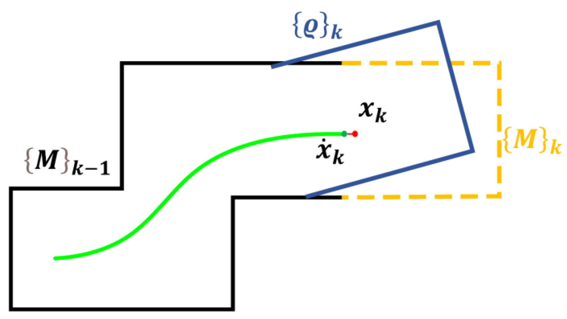
3.5. Map Construction

The high-precision map construction and optimization thread can overlay the scanning point cloud at the current time with the constructed global map point cloud, so as to update the global map incrementally. In order to reduce the cumulative error of point cloud matching caused by pose estimation, this paper matches the current point cloud with the global point cloud, again to optimize the results.
When the point cloud { } k scanned in position pose estimation and LiDAR pose x ˙ k at time t k are received, { } k and { M } k 1 are registered, and the global map { M } k is updated. { } k is converted to the global coordinate system to obtain { ϱ } k , then register { ϱ } k and { M } k 1 . Because the estimated LiDAR pose x ˙ k has error accumulation, the deviation Δ x k of { ϱ } k from the global map { M } k 1 can be solved. Then, the updated global map { M } k and the optimized unmanned parking position and attitude x k at time t k are obtained. Figure 4 is a schematic diagram of the map construction and optimization, in which the black line is the constructed global point cloud; the blue line is the point cloud currently scanned in the global coordinate system, corresponding to the LiDAR scanning at the green point; the yellow line is the optimized laser point cloud, which corresponds to the optimization of the LiDAR posture by laser point cloud scanning at the red point.

3.6. Closed Loop Detection

The closed loop module detects whether the trajectory of the carrier is closed, that is, whether the carrier returns to the previous position. If a closed loop is formed, the ICP algorithm is used to register the current feature point with the feature point cloud at the closed loop to obtain the relative pose relationship t. The closed-loop detection factor is directly input into the factor graph. In this paper, a closed-loop detection method based on Euclidean distance is adopted. By detecting the previous state close to the current key frame in Euclidean space, the pose transformation relationship is obtained by scan matching, and it is added to the factor graph as a closed-loop factor.

3.7. Factor Graph Optimization

The overall framework of the system is shown in Figure 5. The system uses the observations of the sensors to estimate the robot state and its trajectory. The state estimation problem can be expressed as a problem. In this paper, a factor graph is used to model the problem. Under the assumption of a Gaussian noise model, the inference for the maximum posteriori problem is equivalent to solving the nonlinear least squares problem. The odometry framework established based on the factor graph in this paper includes four types of factors: the starting factor, registration factor, IMU factor and closed-loop factor. When the change of the unmanned vehicle posture exceeds the set threshold, a new robot state node will be added to the factor graph for incremental smoothing and mapping by the use of a Bayesian tree. Assuming that the initial state is X 0 , the map building module inserts the registration factor into the factor map corresponding to 𝓇 i Σ i 2 in Equation (3).
𝓇 i = ( x i x i 1 ) T ¯ ( i , i 1 )
The IMU pre-integration module inserts the IMU factor into the factor graph, corresponding to 𝓇 ( i , j ) Σ ( i , j ) 2 in Equation (3):
𝓇 ( i , j ) = ( x i x j )   ( i , j )
The closed-loop detection module inserts the closed-loop factor into the factor graph, corresponding to 𝓇 ( i , j ) Σ ( i , j ) 2 in Equation (3):
𝓇 ( i , j ) = ( x i x j ) T ¯ ( i , j )
where represents the inverse operation of the pose transformation. Whenever new nodes are inserted into the factor graph, the affected nodes are identified and only optimized and updated, so as to maintain the fully optimized sparse characteristics and realize multi-sensor fusion positioning and mapping.

4. Experimental Verification

In order to objectively verify the performance and accuracy of the visual inertial and LiDAR simultaneous localization and mapping (VIAL-SLAM) algorithm proposed in this paper, we conducted mapping and localization experiments in a campus environment and an urban road environment, respectively, and compared them with the FAST-LIO algorithm and the LIO-LIVOX algorithm. The two environments were equipped with different hardware equipment. The campus environment was equipped with an industrial computer with Xeon CPU E3-1275 on the Pix wire control site, while the urban environment was equipped with a laptop computer with I7 10700F. The operating system used the robot operating system (ROS) in Ubuntu18.04. The sensors are divided into LIVOX LIDAR, vision sensor ZED and RTK for inertial navigation. In the campus environment and the urban environment, the sensor parameters were kept consistent to eliminate the influence of the sensors on the experimental results.

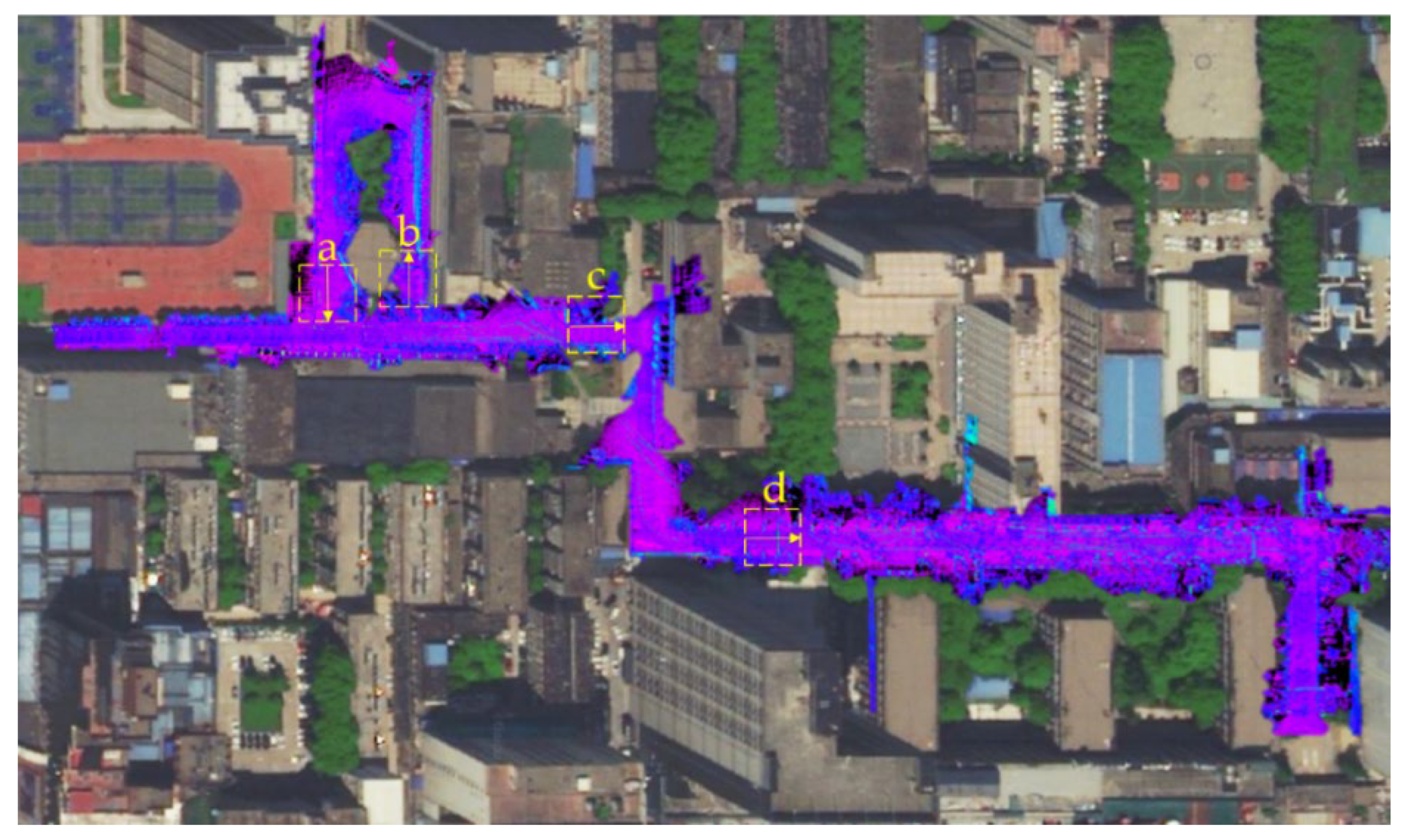
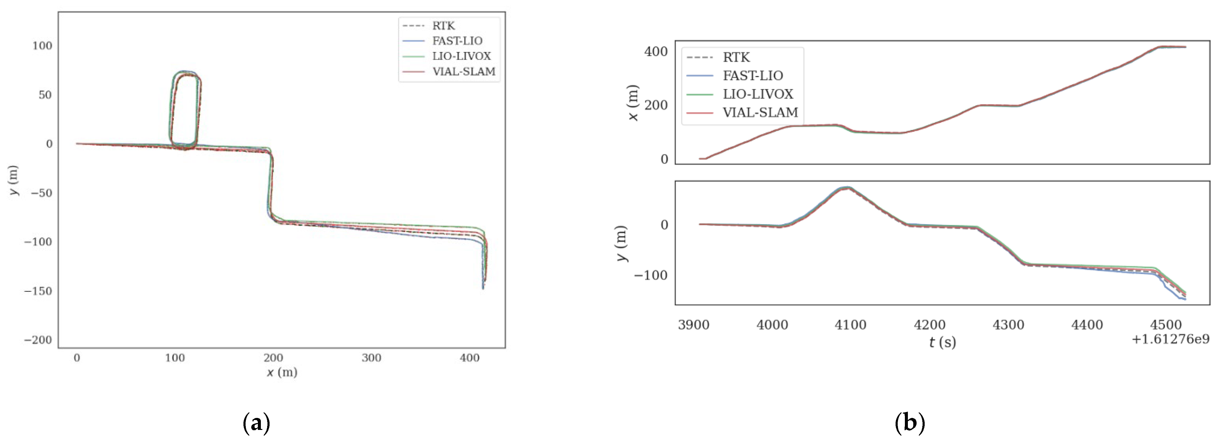
4.1. School Environment Test

We controlled the Pix wire control site to build an internal map at the school. The experimental mileage was about 0.75 Km, the time was 600 s, and the average speed was 4.5 Km/h. The point cloud map constructed in the campus environment was superimposed on the real map, as shown in Figure 6. The specific drawing effects of a, b, c, and d in Figure 6 are shown in Figure 7, and the direction of the arrow indicates the moving direction of the vehicle. Figure 8a is the trajectory diagram of the mapping process, in which the RTK trajectory as the reference is a gray dashed line, the FAST-LIO trajectory is blue, the LIO-LIVOX trajectory is green, and the VIAL-SLAM trajectory is red. At the same time, the comparison of the x-axis and y-axis on the time series is plotted in Figure 8b.
It can be seen from the figure that the VIAL-SLAM proposed in this paper has the smallest error. In order to further evaluate the positioning results, the Absolute Pose Error (APE) index in the EVO evaluation tool [24] is used to evaluate the system performance. Comparing the VIAL-SLAM algorithm, FAST-LIO algorithm and LIO-LIVOX algorithm with the benchmark RTK, the changes of the APE in the time series are shown in Figure 8c, and the error distribution status of the APE is shown in Figure 8d. Table 1 calculates the error ratio of different algorithms in the campus environment in detail. It can be seen from the results that our algorithm, VIAL-SLAM, has excellent positioning effects.

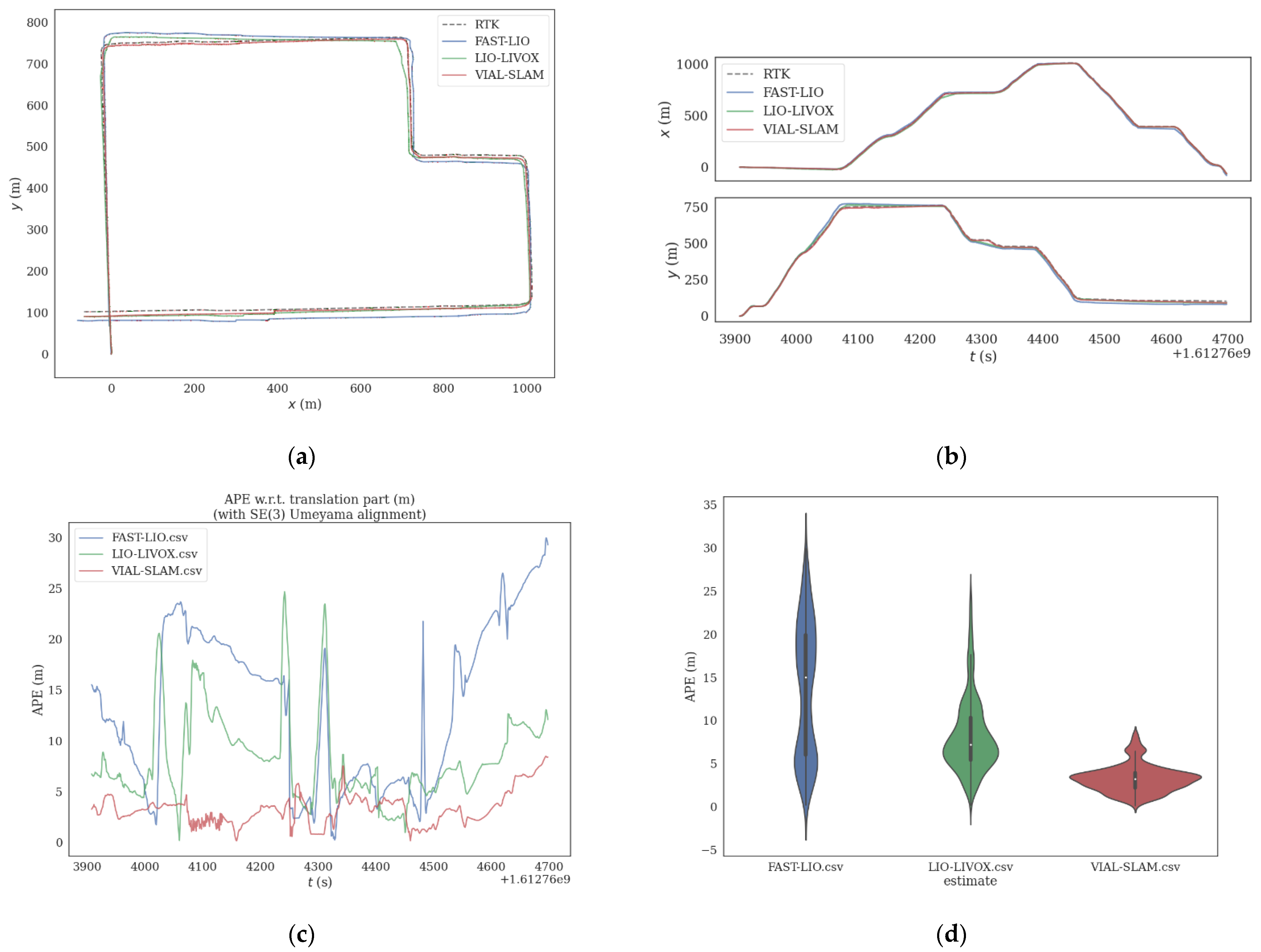
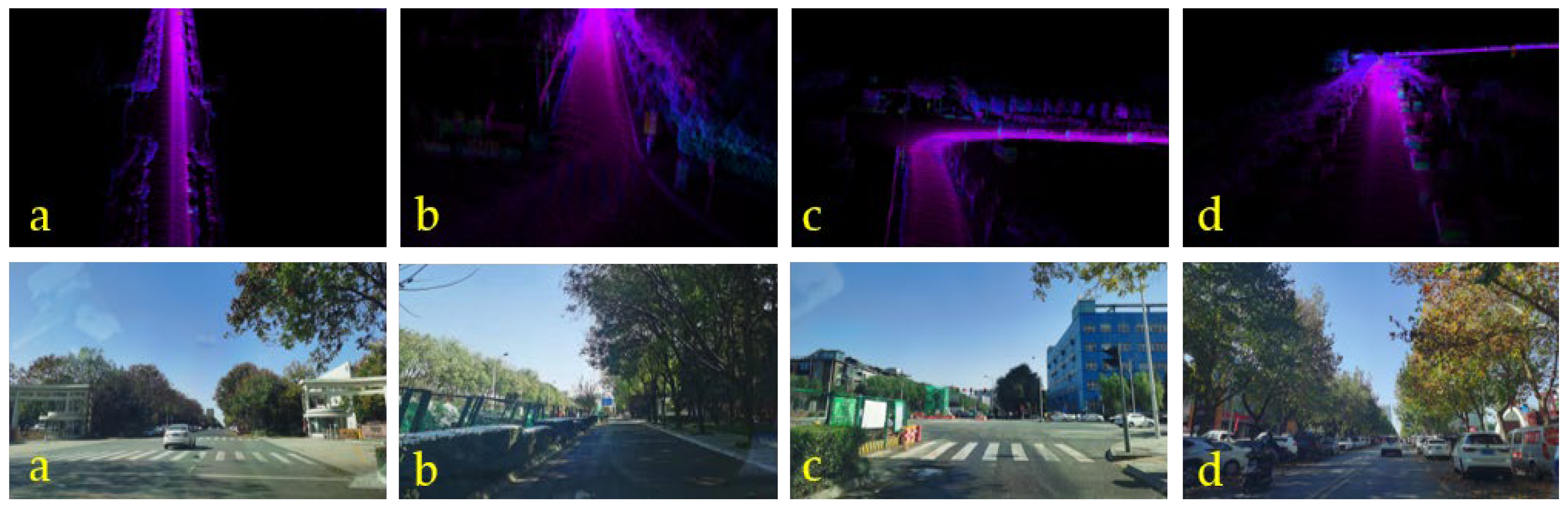
4.2. Real Urban Road Environment Test

In order to verify the system’s autonomous positioning and map construction performance in the real urban road environment, we installed the vision sensor ZED, Lidar sensor LIVOX and inertial navigation RTK on the actual vehicle, as shown in Figure 9.
The mileage of the experiment was about 3.3 km; it took 800 s, and the average speed was 14.85 Km/h. As shown in Figure 10, this article superimposed the results of automatic positioning and map construction on the real map for visual comparison. The specific rendering effects of a, b, c, and d in Figure 10 are shown in Figure 11. The arrow direction indicates the moving direction of the vehicle. According to the result, it can be found that the map constructed in the urban road environment basically matches the real road.
The trajectory estimated by VIAL-SLAM is shown in red in Figure 12a, the trajectory estimated by FAST-LIO is blue, the trajectory estimated by LIO-LIOVX is green, and the reference provided by RTK is gray. The comparison of the x-axis and y-axis in the time series is plotted in Figure 12b, and it can be found that the VIAL-SLAM proposed in this paper is closer to the benchmark RTK. In order to evaluate the positioning accuracy of the system, the absolute positioning accuracy the APE is used for the error calculation and analysis. The autonomous positioning error evaluation results and error distribution status are shown in Figure 12c,d, respectively. Table 2 records the position error ratio of the VIAL-SLAM algorithm, the FAST-LIO algorithm and the LIO-LIVOX algorithm proposed in this paper. The position error rate of the FAST-LIO algorithm and the LIO-LIOVX algorithm are 0.478% and 0.278%, respectively, while the position error rate of VIAL-SLAM is only 0.107%. Compared with FAST-LIO and LIO-LIVOX, it is reduced by 71.43% and 61.51%. The results show that the algorithm still has good performance in the urban road environment.

5. Conclusions

This paper presented a slam system integrating LIDAR IMU vision for autonomous positioning and high-precision map construction in complex environments. The proposed system combines the visual image information, LIDAR point cloud and IMU data. After the point cloud alignment and registration, the pose estimation was carried out and the motion trajectory was optimized by the factor graph. In the system, closed-loop detection was used to eliminate the cumulative error. The point cloud map was registered and updated through the motion estimation and laser point cloud data to build a high-precision map. The algorithm was tested in a campus environment and an urban road environment. Furthermore, we compared it with the FAST-LIO algorithm and the LIO-LIVOX algorithm. The experimental results show that the proposed VIAL-SLAM can achieve accurate autonomous positioning and high-precision map construction in complex environments, and still has high accuracy and robustness.

Author Contributions

Conceptualization, C.Z. and L.L.; investigation, L.L.; methodology, C.Z. and L.L.; project administration, X.M. and R.Z.; resources, X.M. and Z.S.; software, L.L., R.Z. and Z.G.; supervision, X.M.; validation, C.Z.; writing—original draft, L.L.; writing—review and editing, L.L. and Z.G. All authors have read and agreed to the published version of the manuscript.

Funding

This research was funded by the National Natural Science Foundation of China: Research on the Integrated Control Method of the Lateral Stability of Distributed Drive Mining Electric Vehicles (51974229), Shaanxi provincial Department of Education Science and Technology plan Project enterprise joint fund (2019JLP-06), Shaanxi Province Innovative Talent Promotion Plan-Science and Technology Innovation Team (2021TD-27) and The National Key Research and Development Program, China (No. 2018YFB1703402).

Institutional Review Board Statement

Not applicable.

Informed Consent Statement

Not applicable.

Data Availability Statement

Not applicable.

Conflicts of Interest

The authors declare no conflict of interest.

References

  1. Zhao, J.; Li, T.; Yang, T.; Zhao, L.; Huang, S. 2D Laser SLAM with Closed Shape Features: Fourier Series Parameterization and Submap Joining. IEEE Robot. Autom. Lett. 2021, 6, 1527–1534. [Google Scholar] [CrossRef]
  2. Rublee, E.; Rabaud, V.; Konolige, K.; Bradski, G. ORB: An efficient alternative to SIFT or SURF. In Proceedings of the 2011 IEEE International Conference on Computer Vision (ICCV 2011), Barcelona, Spain, 6–13 November 2011; pp. 2564–2571. [Google Scholar]
  3. Mur-Artal, R.; Montiel, J.M.; Tardos, J.D. ORB-SLAM: A versatile and accurate monocular SLAM system. IEEE Trans. Robot. 2015, 31, 1147–1163. [Google Scholar] [CrossRef] [Green Version]
  4. Mur-Artal, R.; Tardós, J.D. ORB-SLAM2: An Open-Source SLAM System for Monocular, Stereo, and RGB-D Cameras. IEEE Trans. Robot. 2017, 33, 1255–1262. [Google Scholar] [CrossRef] [Green Version]
  5. Usenko, V.; Engel, J.; Stückler, J.; Cremers, D. Direct visual-inertial odometry with stereo cameras. In Proceedings of the 2016 IEEE International Conference on Robotics and Automation (ICRA), Stockholm, Sweden, 16–21 May 2016; pp. 1885–1892. [Google Scholar]
  6. Qin, T.; Cao, S.; Pan, J.; Shen, S. A general optimization-based framework for global pose estimation with multiple sensors. arXiv 2019, arXiv:1901.03642. [Google Scholar]
  7. Campos, C.; Elvira, R.; Rodriguez, J.J.G.; Montiel, J.M.M.; Tardos, J.D. ORB-SLAM3: An Accurate Open-Source Library for Visual, Visual–Inertial, and Multimap SLAM. IEEE Trans. Robot. 2021, 37, 1874–1890. [Google Scholar] [CrossRef]
  8. Qin, T.; Li, P.; Shen, S. Vins-mono: A robust and versatile monocular visual-inertial state estimator. IEEE Trans. Robot. 2018, 34, 1004–1020. [Google Scholar] [CrossRef] [Green Version]
  9. Zhang, J.; Singh, S. Low-drift and Real-Time Lidar Odometry and Mapping. Auton. Robot 2017, 41, 401–416. [Google Scholar] [CrossRef]
  10. Shan, T.; Englot, B. LeGO-LOAM: Lightweight and Ground-Optimized Lidar Odometry and Mapping on Variable Ter-rain. In Proceedings of the 2018 IEEE/RSJ International Conference on Intelligent Robots and Systems (IROS), Madrid, Spain, 1–5 October 2018; pp. 4758–4765. [Google Scholar]
  11. Shan, T.; Englot, B.; Meyers, D.; Wang, W.; Ratti, C.; Rus, D. LIO-SAM: Tightly-coupled Lidar Inertial Odometry via Smoothing and Mapping. In Proceedings of the IEEE/RSJ International Conference on Intelligent Robots and Systems, Las Vegas, NV, USA, 25–29 October 2020. [Google Scholar]
  12. Ye, H.; Chen, Y.; Liu, M. Tightly coupled 3d lidar inertial odometry and mapping. In Proceedings of the 2019 International Conference on Robotics and Automation (ICRA), Montreal, QC, Canada, 20–24 May 2019; pp. 3144–3150. [Google Scholar]
  13. Zhao, S.; Fang, Z.; Li, H.L.; Scherer, S. A robust laser-inertial odometry and mapping method for large-scale highway environ-ments. In Proceedings of the 2019 IEEE/RSJ International Conference on Intelligent Robots and Systems (IROS), Macau, China, 3–8 November 2019; pp. 1285–1292. [Google Scholar]
  14. Geneva, P.; Eckenhoff, K.; Yang, Y.; Huang, G. LIPS: Lidar-Inertial 3d plane slam. In Proceedings of the 2018 IEEE/RSJ International Conference on In-telligent Robots and Systems (IROS), Madrid, Spain, 1–5 October 2018; pp. 123–130. [Google Scholar]
  15. Bry, A.; Bachrach, A.; Roy, N. State estimation for aggressive flight in GPS-denied environments using onboard sensing. In Proceedings of the 2012 IEEE International Conference on Robotics and Automation, Saint Paul, MN, USA, 14–18 May 2012; pp. 1–8. [Google Scholar]
  16. Debeunne, C.; Vivet, D. A review of visual-LiDAR fusion based simultaneous localization and mapping. Sensors 2020, 20, 2068. [Google Scholar] [CrossRef] [PubMed] [Green Version]
  17. Zhang, J.; Singh, S. Visual-lidar odometry and mapping: Low-drift, robust, and fast. In Proceedings of the 2015 IEEE International Conference on Robotics and Automation (ICRA), Seattle, WA, USA, 26–30 May 2015; pp. 2174–2181. [Google Scholar]
  18. Seo, Y.; Chou, C.C. A tight coupling of vision-lidar measurements for an effective odometry. In Proceedings of the 2019 IEEE Intelligent Vehicles Symposium (IV), Paris, France, 9–12 June 2019; pp. 1118–1123. [Google Scholar]
  19. Jiang, G.; Yin, L.; Jin, S.; Tian, C.; Ma, X.; Ou, Y. A Simultaneous Localization and Mapping (SLAM) Framework for 2.5D Map Building Based on Low-Cost LiDAR and Vision Fusion. Appl. Sci. 2019, 9, 2105. [Google Scholar] [CrossRef] [Green Version]
  20. Lin, J.; Zhang, F. Loam livox: A fast, robust, high-precision LiDAR odometry and mapping package for LiDARs of small FoV. In Proceedings of the 2020 IEEE International Conference on Robotics and Automation (ICRA), Paris, France, 31 May–31 August 2020; pp. 3126–3131. [Google Scholar]
  21. Chen, S.; Zhou, B.; Jiang, C.; Xue, W.; Li, Q. A LiDAR/Visual SLAM Backend with Loop Closure Detection and Graph Optimization. Remote Sens. 2021, 13, 2720. [Google Scholar] [CrossRef]
  22. Wang, W.; Liu, J.; Wang, C.; Lin, B.; Zhang, C. DV-LOAM: Direct visual lidar odometry and mapping. Remote Sens. 2021, 13, 3340. [Google Scholar] [CrossRef]
  23. Calonder, M.; Lepetit, V.; Strecha, C.; Fua, P. Brief: Binary Robust Independent Elementary Features; European conference on computer vision; Springer: Berlin/Heidelberg, Germany, 2010; pp. 778–792. [Google Scholar]
  24. Sturm, J.; Engelhard, N.; Endres, F.; Burgard, W.; Cremers, D. A benchmark for the evaluation of RGB-D SLAM systems. In Proceedings of the 2012 IEEE/RSJ International Conference on Intelligent Robots and Systems, Vilamoura-Algarve, Portugal, 7–12 October 2012; pp. 573–580. [Google Scholar]
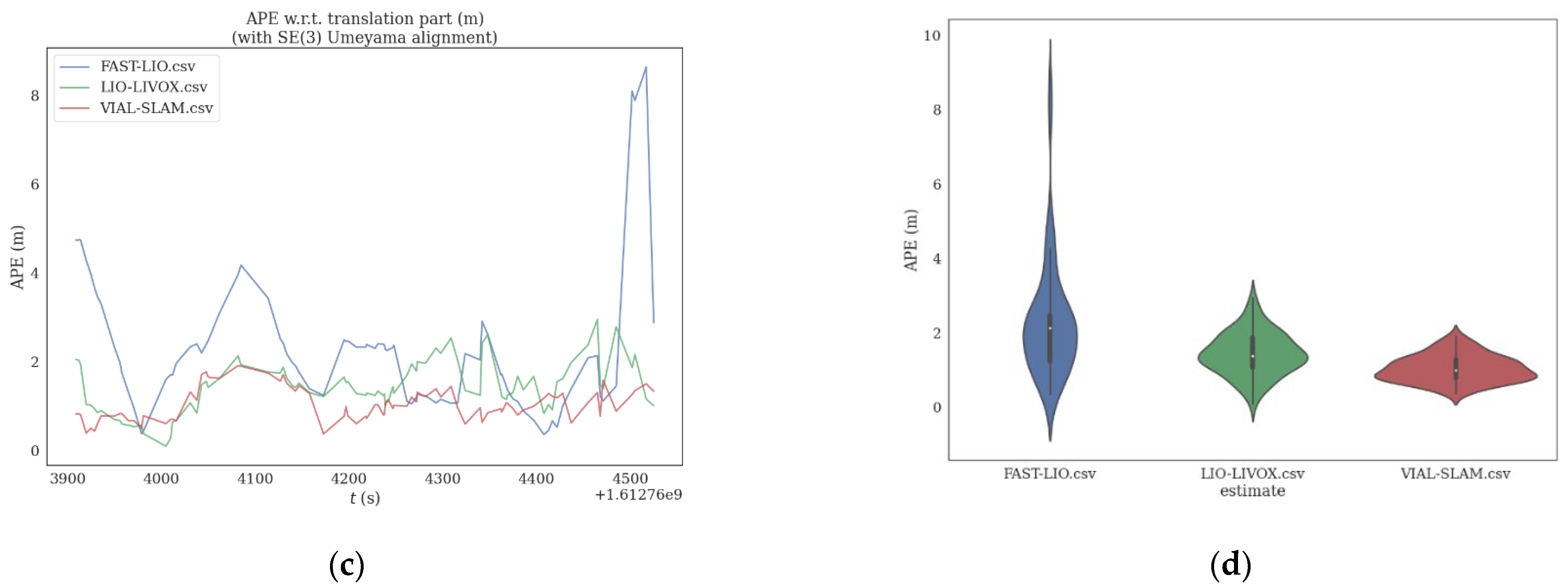
Figure 1. The overview of the system.
Wevj 12 00261 g001
Figure 2. Feature extraction and segmentation. (a) The original point cloud; (b) ground points and split points; (c) the edge point and plane point in i e and i f ; (d) the edge point and plane point in i e and i f .
Wevj 12 00261 g002
Figure 3. Fusion results of the visual and laser features.
Wevj 12 00261 g003
Figure 4. Map construction and optimization.
Wevj 12 00261 g004
Figure 5. Factor diagram optimization process.
Wevj 12 00261 g005
Figure 6. The VIAL-SLAM map aligned with Google Earth.
Wevj 12 00261 g006
Figure 7. The mapping results in the campus environment; (ad) shows the point cloud map of the LiDAR and the matched image information. The shooting position is shown in four places (ad) in Figure 6.
Wevj 12 00261 g007
Figure 8. Error analysis diagram. (a) Trajectory comparison; (b) trajectory comparison on the x-axis and y-axis; (c) error comparison; (d) error estimate.
Wevj 12 00261 g008aWevj 12 00261 g008b
Figure 9. The experimental equipment was completed by loading LIVOX LiDAR, a camera and RTK onto the real vehicle, and the driver drove the vehicle through the designated road section.
Wevj 12 00261 g009
Figure 10. The VIAL-SLAM map aligned with Google Earth.
Wevj 12 00261 g010
Figure 11. The mapping results on an urban road; (ad) show the point cloud map of the lidar and the matched image information. The shooting position is shown in four places (ad) in Figure 10.
Wevj 12 00261 g011
Figure 12. Error analysis diagram. (a) Trajectory comparison; (b) trajectory comparison on the x-axis and y-axis; (c) error comparison; (d) error estimate.
Wevj 12 00261 g012
Table 1. The campus environment test results.
Error TermVIAL-SLAMLIO-LIVOXFAST-LIO
Root mean square error0.67 m1.49 m2.92 m
Mean error0.56 m1.35 m2.49 m
Error ratio0.095%0.213%0.417%
Table 2. The autonomous positioning test results in the urban road environment.
Error TermVIAL-SLAMLIO_LIVOXFAST-LIO
Root mean square error3.54 m9.18 m15.77 m
Mean error3.08 m7.92 m13.5 m
Error ratio0.107%0.278%0.478%
Publisher’s Note: MDPI stays neutral with regard to jurisdictional claims in published maps and institutional affiliations.

