Article

Multistage and Dynamic Layout Optimization for Electric Vehicle Charging Stations Based on the Behavior Analysis of Travelers

1
Shien-Ming Wu School of Intelligent Engineering, South China University of Technology, Guangzhou 510000, China
2
Department of Electrical and Electronic Engineering, Xi’an Jiaotong-Liverpool University, Suzhou 215123, China
*
Author to whom correspondence should be addressed.
World Electr. Veh. J. 2021, 12(4), 243; https://doi.org/10.3390/wevj12040243
Submission received: 10 October 2021 / Revised: 6 November 2021 / Accepted: 11 November 2021 / Published: 15 November 2021

Abstract

:
Electric vehicles (EV) are growing fast in recent years with the widespread concern about carbon neutrality. The development of charging infrastructures needs to be in phase with EV both in terms of quantity and charging time to decrease the range anxiety of EV users and resource waste. This paper proposed a multistage and dynamic layout optimization model based on mixed integer linear programming (MILP) for EV charging stations (CSs) to minimize the total social costs (TSC) consisting of the detour cost of EV users and the construction, relocation, and operating cost of CSs. The charging satisfaction coefficient and M/M/S/K model of queuing theory has been introduced to determine the desirable charging supply. The spatial-temporal distribution of charging demand was modeled based on the behavior analysis of travelers and over the discrete-time intervals for a day. Comparison studies based on the Sioux Falls network reveal that TSC with a multistage optimization strategy will drop 8.79% from that with a one-time optimization strategy. Charging service quality, relocation cost, and road network scales have a significant impact on the optimization results according to the sensitivity analysis.

Graphical Abstract

1. Introduction

The deployment of electric vehicles (EVs) has been growing rapidly in recent years, with the global stock of electric passenger cars reaching 7.2 million units in 2019, 40% higher than that in 2018 [1]. However, the unreasonable layout of EV charging stations (CSs) increases the range anxiety of EV users and seriously impedes the sustainable development of the EV market. Although greater than 85% of EV charging still occurs at home, the availability of public charging infrastructure plays a key role in expanding EV adoption [2]. Global Times reported that many Chinese EV users found it hard to charge their EVs at service zones along highways apart from the normal jams during the National Day holiday, which reflects the current problem that our charging infrastructure needs to improve [3]. This paper focuses on the layout optimization of EV CSs with fast charging piles (FCPs) in a long-term plan.
The detailed analysis of EV users’ behavior and the accurate prediction of the temporal and spatial charging demand distribution are very important for designing a reasonable layout of CSs. Zhang et al. proposed an optimization strategy with the knowledge of the whole day’s vehicle travel pattern provided by the NHTS data to minimize the overall cost [4]. Tian et al. used the cloud model to predict the charging behavior of car owners and found that the charging waiting time without considering the charging behavior of car owners was 27.28% longer than that considering the charging behavior [5]. Xiang et al. propose a spatial-temporal simulation method based on the vehicle-transportation-grid trajectory considering the uncertainty of the user’s driving behavior and charging intention [6]. This paper proposes a model based on the Monte Carlo method to generate the charging demand distribution in the planning area with the analysis of EV users’ behavior and to support the layout optimization model.
With the rapid growth of the number of EVs, the problem of multistage and dynamic layout optimization has been studied extensively in recent years. Xie et al. introduced a multistage chance-constrained stochastic model for optimizing the layout of CSs inside the city and used MILP to decide when and where to lay out CSs and the number of charging piles [7]. Lin et al. proposed a spatial-temporal model to determine the sites and sizes of e-bus charging stations and put forward the strategies for multistage infrastructure planning [8]. Li et al. proposed a multistage and multipath location model to expand the network of CSs dynamically and satisfy the increasing demand of the O-D tour with consideration of relocation [9]. Typically, the multistage models mentioned above sacrifice the accurate analysis of the charging demand in a day to speed up the calculation time. For instance, the uneven distribution of charging demand in a day was ignored, and the charging demand was regarded as proportional to the EV numbers in the model proposed in [9]. The model proposed in this paper considers the fluctuation of the charging demand in a day by introducing a time interval strategy. The queuing behavior of EV users has also been analyzed.
The layout optimization of CSs is a complicated problem involving many stakeholders such as EV users, CS investors and power grid, etc. [10]. The objective was to minimize the investment costs, subject to satisfying the EV charging demand in the planning model proposed by Zhang et al. [11], but it was hard to guarantee that the driving range constraints would be met. He et al. found that the p-median solution focusing on the interests of EV users was more effective than two other models in the sense that the CSs were closer to the communities with higher charging demand [12], but the investment willingness of CS investors would be impeded due to the high initial construction cost of CS [13]. This paper proposes a model aimed at minimizing the total social cost (TSC) to balance the interests of EV users and CS investors.
In order to solve the non-linear and NP-hard problem of large-scale location optimization, some heuristic optimization algorithms are applied in the layout optimization of EV CSs, such as genetic algorithm (GA) [14], iterative greedy heuristic [15], simulated annealing algorithm (SA) [16], etc. Although heuristic algorithms could obtain the suboptimal solution within a relatively short time, they would fall into a local optimal solution when the dimension of the decision variables becomes high, for which it is hard to ensure the accuracy and reliability of the solution. In addition to heuristic optimization algorithms, some methods such as branch-and-bound methods [11] and transforming the model into a mixed-integer second-order cone programming [8] can also solve the non-linear or NP-hard hard problem in some conditions. This paper proposed a two-layer structure to decouple the CS layout problem in the long-term planning and queuing problem in relatively short time intervals. The capacity of CSs is ensured by introducing the charging service satisfaction coefficient and piecewise linear method (PWL) and the optimization problem is formulated as mixed integer linear programming (MILP) to avoid the non-linear or non-convex problem caused by the queuing theory in [4,14].
Based on the above analysis, it could be known that the considerations about the behavior of EV users and the fluctuation of the charging demand in a day are not enough in the multistage layout optimization of CSs. This paper proposed a multistage layout optimization model for CSs aimed at minimizing the TSC and solving with MILP with a particular consideration of EV users’ behavior.
This paper intends to make the following two key contributions.
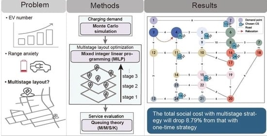
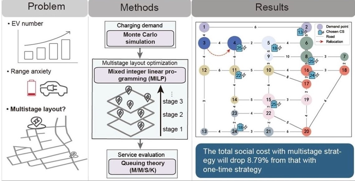
  • First, multistage CS layout optimization is studied comprehensively with the dynamic EV charging demands of one day. The proposed method cannot only optimize the layout of CSs considering the numbers of EVs at different stages but also ensure the service quality by satisfying the charging demand at different time intervals in a day.
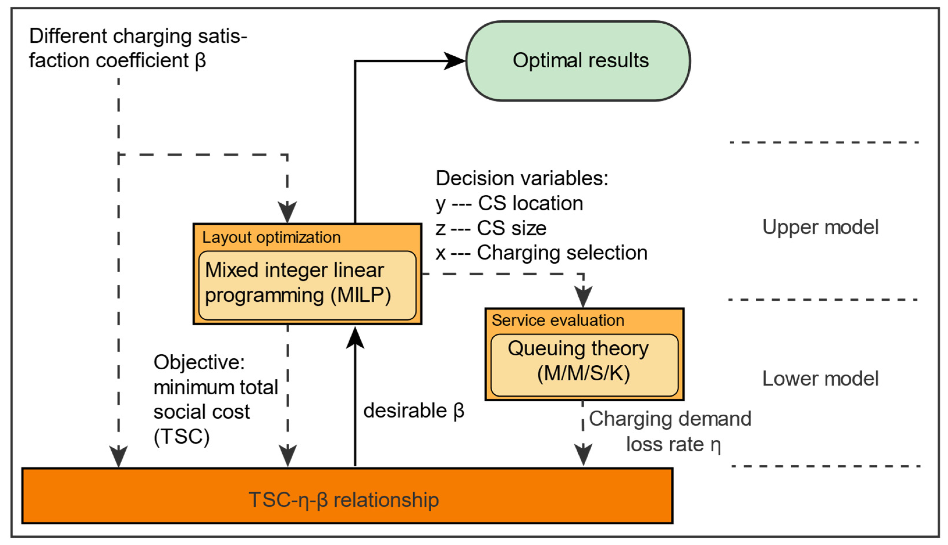
  • Second, we designed a two-layer model to avoid the non-linear characteristics caused by the queuing phenomenon, which can improve the computational speed and consider the important queuing phenomenon during EV charging in a large road network.
The rest of this paper is organized as follows. In Section 2, we introduce the generative model of charging demand distribution based on the Monte Carlo method with the analysis of travel and charging behavior of EV users. Section 3 proposes a two-layer layout model for CSs based on MILP and a M/M/S/K model of queuing theory aimed at minimizing TSC. In Section 4, the case based on the Sioux Falls network is studied and the optimal layout results are analyzed. At last, we draw a conclusion of this paper and put forward the future work in Section 5.

2. Charging Demand Distribution

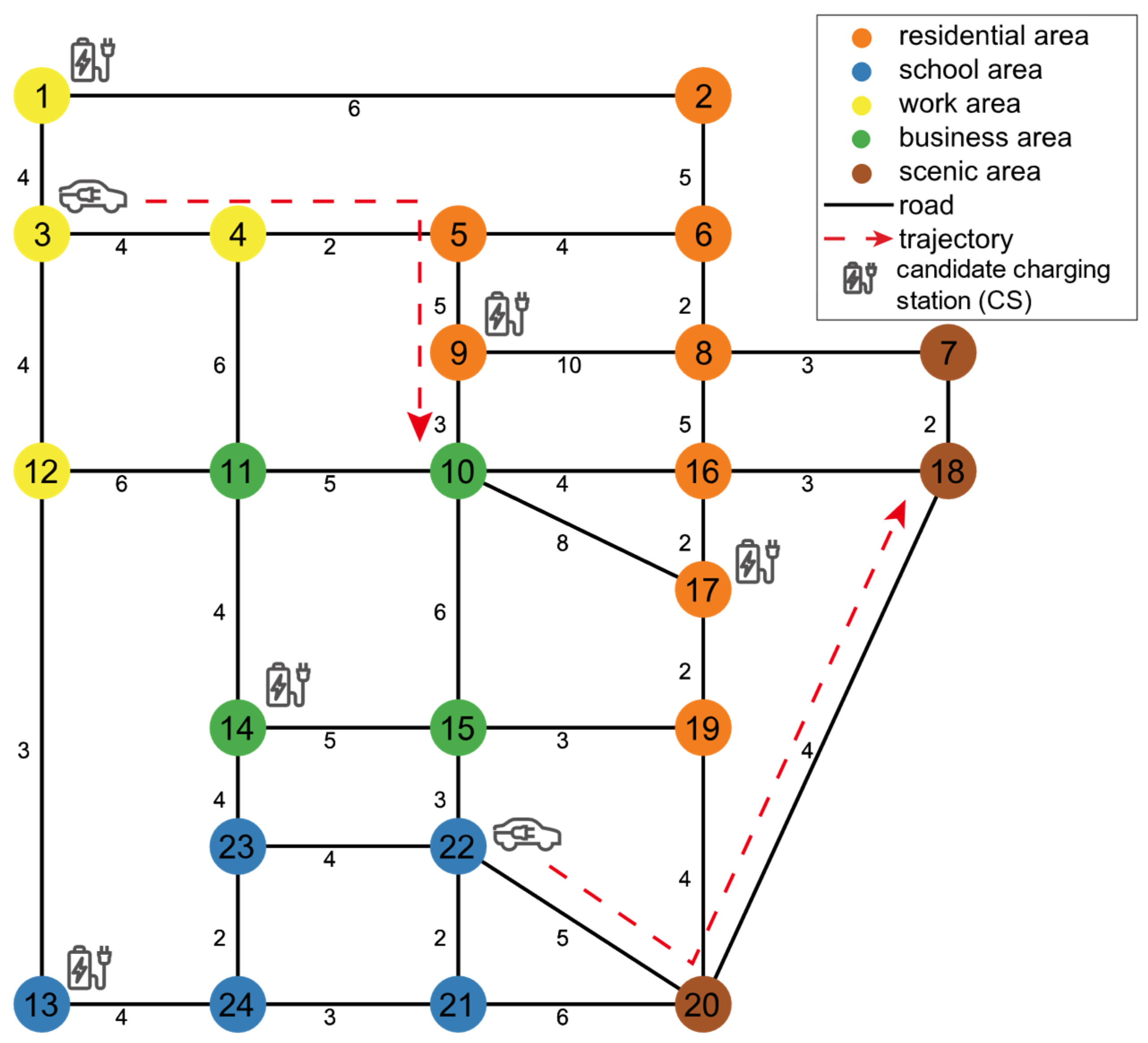
2.1. Problem Description

A schematic diagram based on the Sioux Falls road network [17] is used for illustrating the question more clearly, as shown in Figure 1. The locations of candidate charging stations (CCSs) are assumed to be on the road crossings due to their stronger ability to capture traffic flow. Every EV trajectory represented by the red dash line is divided into several points (road crossings, also known as demand points) and the EV user will decide whether to choose a CS for charging at these demand points according to the state of charge (SOC) of the EV battery.
The objective is catching the traffic flow and charging demand at each demand point and each time interval in the planning area, and there are generally two ways to obtain the information; data-driven method with full information and simulation method with limited information. The information of the road network and UFZs is easy to access, but the data of residents’ travel trajectories and the SOC of EV batteries is hard due to privacy protection. Taxi GPS data were used in some studies, but taxies cannot represent all types of EVs, which causes the deviation of the charging demand. This paper proposes a model based on the Monte Carlo method to generate the spatial-temporal distribution of charging demand with the information of the road network, UFZs, the temporal travel patterns of EVs and the population scale.

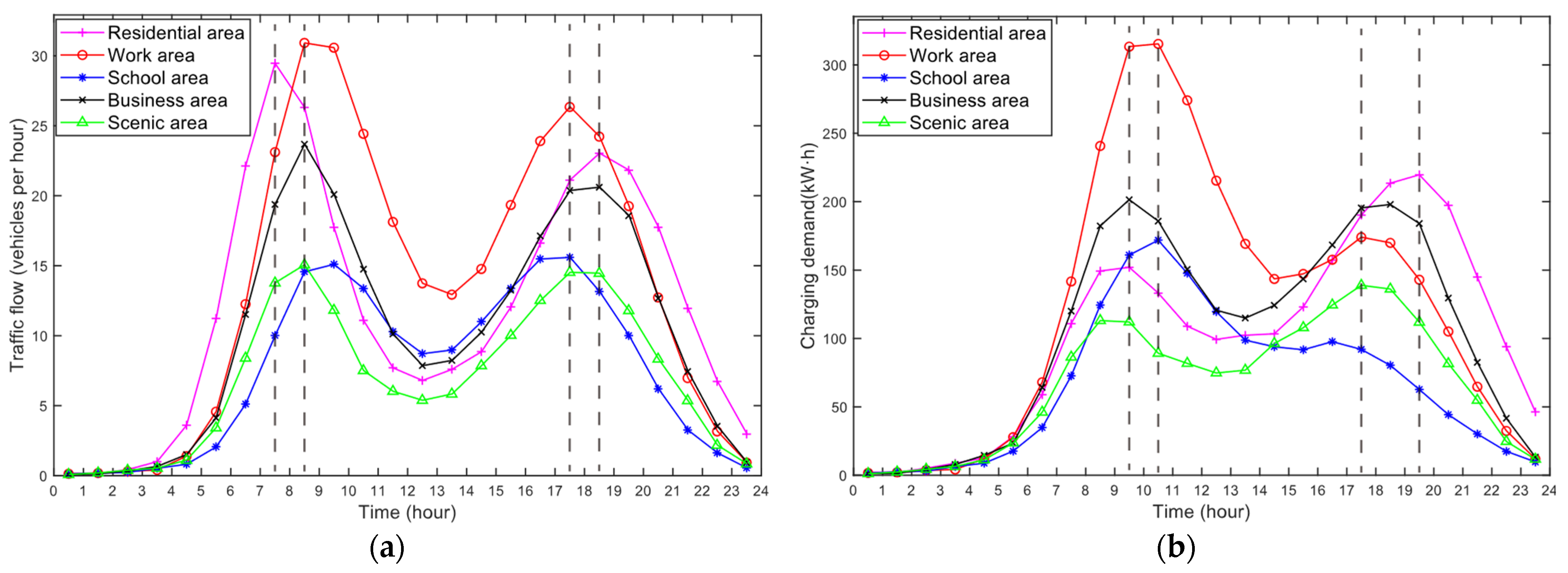
2.2. Travel Behavior Analysis

According to the research report on EV use in England [18], 61% of EVs are used for commuting, which means they will go to workplaces or schools in the morning and back home in the afternoon, and 39% of EVs are used for non-commuting, which means travel trajectories are uncertain. The EV temporal travel pattern in a day is in accordance with the normal distributions with different coefficients according to the research findings demonstrated in [19], which will be used to ensure the travel time in the Monte Carlo simulation although the EV temporal travel patterns in different areas will be influenced by living habits of residents, traffic condition, and distribution of UFZs, etc.

2.3. Charging Behavior Analysis

The fast charging process will stop once the EV battery is charged to the upper limit of the state of charge ( S O C ¯ ) for the sake of time saving and overcharge protection [11]. Although charging control and management can improve CS operators’ profits from an operating perspective [20,21], EVs are assumed to be charged at rated power in this paper in consideration of the immature technology and the convenience of modeling. When the SOC is below the lower limit of the state of charge ( S O C ¯ ) during the travel, EV will warn the owner of emergency charging to avoid the adverse consequences. This article assumes the initial SOC of commuting EVs in a day are S O C ¯ because EV users prefer to charge in the evening with household charging piles or slow charging piles installed in the residential area for low charging prices and less harm to EV battery. The initial SOC of non-commuting EVs in a day follow the uniform distribution [ S O C ¯ , S O C ¯ ] for the randomness of travel trajectories.

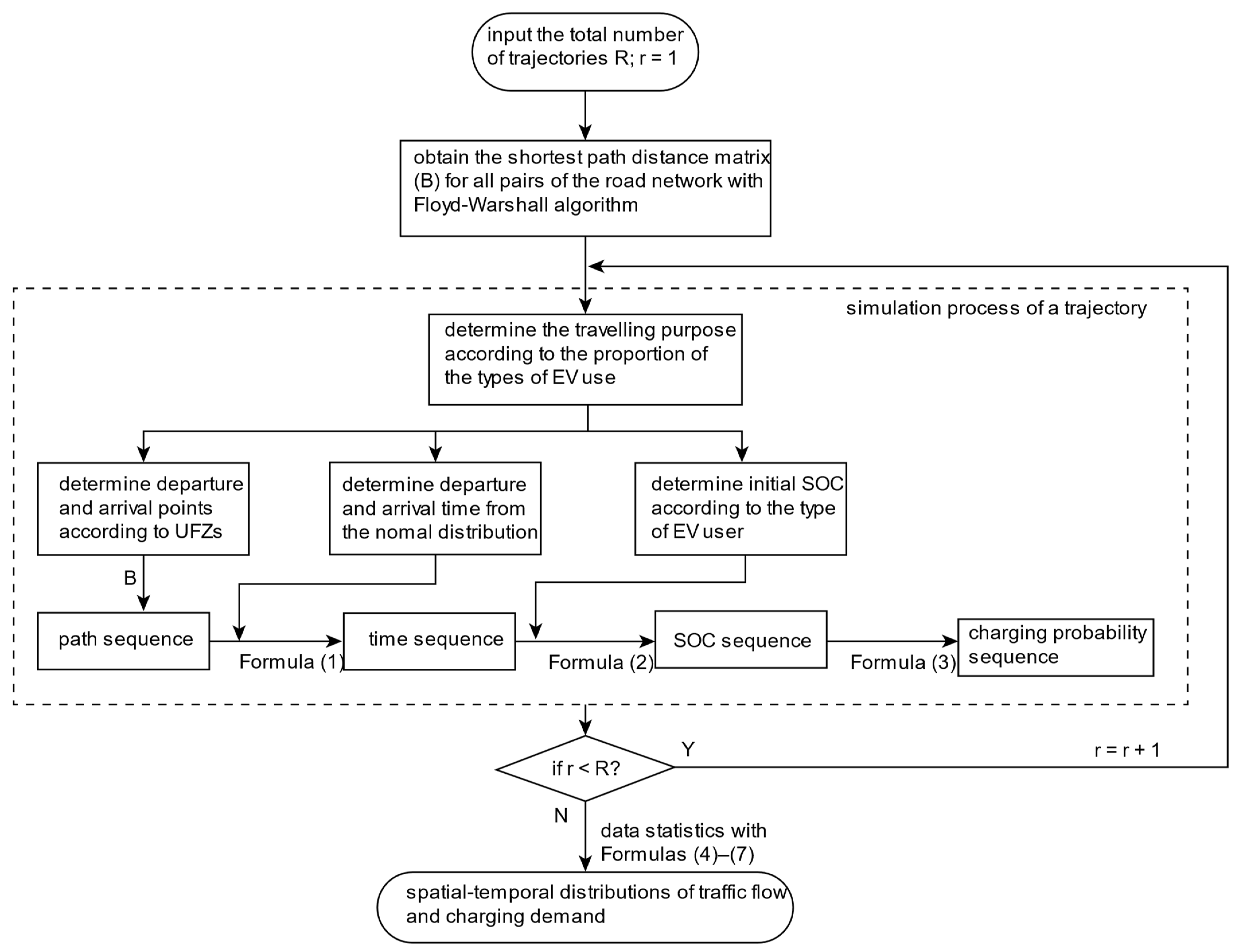
2.4. Monte Carlo Method

The simulation of traffic flow and charging demand distribution based on the Monte Carlo method is shown in Figure 2, and the nomenclature can be seen before Appendix A.
t s r = t 1 r + ( t S r r t 1 r ) d s r d S r r
S O C s r = S O C 1 r ( t s r t 1 r ) V γ C m
P s r = { 1 0.5 · S O C s r ,   0 S O C s r < 0.2 7 6 4 3 · S O C s r ,   0.2 S O C s r < 0.8 0.5 0.5 · S O C s r ,   0.8 S O C s r 1
Every trajectory will be simulated in our model, whose departure point and arrival point are selected from corresponding sets of points with the same kind of UFZs randomly according to the traveling purpose, e.g., from a point in the residential area to a point in the work area. This paper assumes EV users will choose the shortest path generated by the Floyd–Warshall algorithm [22]. The departure and arrival moments are given by normal distributions [18] and the time of other points on the trajectory are ensured by the Formula (1). The SOC sequence is determined by the initial SOC and the electrical energy consumed along the travel, as shown in Formula (2). The relationship between charging probability and SOC has been simplified as a piecewise linear function according to the survey results [4], as shown in Formula (3). Some constraints will be added to make the trajectory more realistic: regenerating the time sequence if t 1 r and t S r r are not within [ 0 , 24 ] , and cutting off the trajectory if S O C s r < 0 .
h s , i , t r = { 1 , i f   l s r = i , t 1 < t s r t 0 ,   otherwise
δ s r = { 1 ,                                         if   s = 1 s = 1 s 1 ( 1 P s r ) ,   if   s   >   1
W i , t = r = 1 R s = 1 S r h s , i , t r δ s r P s r
D i , t = r = 1 R s = 1 S r h s , i , t r δ s r P s r ( S O C ¯ S O C s r ) C m
After the path, time, SOC, and charging probability sequences of each trajectory have been simulated, the traffic flow (vehicles per hour) and charging demand (kW·h) at each demand point and each time interval will be counted in a statistical sense according to Formulas (4) and (7). In Formula (4), h s , i , t r is a binary variable to count whether the point on the trajectory is at a certain demand point and a certain time interval. It is a sequential decision process for an EV to charge during the travel. The EV user will decide whether to charge or not at the first point according to P 1 r , if not, the EV user will drive to the next point and make a decision again, and the decision process will be repeated in this way until the EV is charged. This process can be modeled in a statistical sense, as shown in Formulas (6) and (7). Based on the above statistics, spatial-temporal distributions of traffic flow and charging demand will provide a reliable data basis for the subsequent layout optimization of CSs.

3. Mathematical Modeling

A two-layer model has been built to optimize the locations and sizes of CSs in long-term planning, as shown in Figure 3. For the upper model, the layout problem of EV CSs is constructed as a MILP model with a presumed charging satisfaction coefficient β , which controls the number of FCPs and the service quality of CSs. The charging and waiting process was modeled as a multi-service window waiting system according to the M/M/S/K model of queuing theory in the lower model. Charging demand loss rate η can be acquired by the M/M/S/K model with the layout optimization results of CSs and charging selection of EV users as input information. Charging demand loss means EVs with charging demand will leave the CS if FCPs and waiting spaces are fully occupied, which can evaluate the charging service quality of the CS.

3.1. Mixed Integer Linear Programming (MILP) Model

3.1.1. Total Social Cost

min k = 1 K ( α J E V , k + ( 2 α ) J C S , k )
where the objective function is to optimize the locations of CSs from the candidate charging stations (CCSs) to minimize the TSC, which includes the detour cost of EV users from the demand point to the charging station and the construction, relocation and operating cost of CSs. Minimizing the TSC means fewer resources, leading to the reduction in EV users’ range anxiety. The ratio relationship between these two costs is controlled by α [ 0 , 2 ] according to the decision maker. In this paper, α is set as 1 without the loss of generality.
J E V , k = 365 t = 1 T i = 1 N j = 1 M W i , t , k F i , j , t x i , j , k
where one stage is set as one year in our model although other factors can be a standard for dividing stages, such as EV numbers and other time scales. Formula (9) shows the composition of the detour cost of EV users at stage k , where W i , t , k and F i , j , t are fixed according to the Monte Carlo simulation and road network. A day is divided into 24 pieces by time step Δ T leading to a more accurate description of the charging demand distribution and the congestion of roads. Minimizing the detour cost implies the EV users will choose the CS for charging as close as possible.
F i , j , t = d i , j F V i , j , t
In Constraint (10), the time cost of detours is converted into the monetary cost with an average hourly wage, which unifies dimensions and leads to a single objective problem. The average speed of EVs is assumed to be the same, although the speed influenced by the traffic condition may be different in different time intervals of a day.
J C S , k = { ( C c c s + C o c s ) j = 1 M y j , k + ( C c c p + C o c p ) j = 1 M z j , k ,   k = 1 j = 1 M ( J C S , j , k c s + J C S , j , k c p + J C S , j , k c s , r + J C S , j , k c p , r ) ,           k 1
Formula (11) shows the composition of the cost related to CSs at stage k , which can be divided into two conditions, k = 1 and k 1 . There are only construction and operating costs but not relocation cost at stage 1 because of the assumption of no CS at the beginning of the overall planning. The CS may be removed from one location to another at the later stages for some reasons, such as the change of charging demand distribution, the competition between CSs, etc.
J C S , j , k c s = { C c c s ( y j , k y j , k 1 ) , y j , k y j , k 1 0 ( C c c s C r c s ) ( y j , k y j , k 1 ) , y j , k y j , k 1 < 0
J C S , j , k c p = { C c c p ( z j , k z j , k 1 ) , z j , k z j , k 1 0 ( C c c p C r c p ) ( z j , k z j , k 1 ) , z j , k z j , k 1 < 0
J C S , j , k c s , r + J C S , j , k c p , r = C o c s y j , k + C o c s z j , k
In Formula (12),   y j , k = y j , k 1 = 0 and   y j , k = y j , k 1 = 1 represent that the close or open states of CS j are the same at two adjacent stages, leading to a zero cost of construction and relocation. y j , k = 1 , y j , k 1 = 0 represents CS j is newly built so the construction cost will be C c c s . y j , k = 0 , y j , k 1 = 1 represents CS j is removed at stage k and the cost is ( C r c s C c c s ) . Meanwhile, relocation destination will new build a CS and the cost will be C c c s , leading to ( C r c s C c c s ) + C c c s = C r c s as the total cost of a relocation. It needs to be noted that FCPs can be relocated without the relocation of CSs and the explanation about the installation and relocation cost of FCPs in Formula (13) will be omitted for its similarity to Formula (12). The function in Formulas (12) and (13) are non-linear so the piecewise linear method (PWL) with the constraint of a special ordered set type 2 (SOS2) is introduced to solve the non-linear problem [23] and the detailed operation will not be shown in this paper for conciseness. Formula (14) shows the operating and maintenance cost of CSs and FCPs.

3.1.2. Location Constraints

j = 1 M x i , j , k = 1
x i , j , k y j , k
Constraint (15) represents EVs on one demand point can and only can choose one CS for charging, and Constraint (16) ensures the chosen CS is an open CS.
d i , j · x i , j , k < S O C ¯ · C m · γ
Constraint (17) ensures the distance between the demand point and the corresponding chosen CS should not be further than the driving range supported by the lower limit of EV battery, which can control the lower limit of the number of the chosen CCSs and avoid the unbearable distance when the EV goes for charging.

3.1.3. Capacity Constraints

β i = 1 N ( D i , t , k + W i , t , k d i , j γ ) x i , j , k z j , k P c Δ T
Constraint (18) represents that the total power of FCPs in each CS should satisfy the charging demand of EV users and the energy consumed on the way to the CS during time interval Δ T , which can control the minimum number of FCPs. Some charging demand in a time interval cannot be satisfied when β 1 for the uneven EV arrivals and the investment will increase when β > 1 . The control of β is crucial to balance the investment and charging demand loss, whose relationship will be quantified and discussed in Section 4.3.1.
z j , k G j , k · y j , k
Constraint (19) limits the location and number of FCPs. G j , k represents the upper limit of FCPs determined by the capacity of land and the distribution grid.

3.1.4. Other Constraints

j = 1 M y j , k j = 1 M y j , k + 1
j = 1 M z j , k j = 1 M z j , k + 1
x i , j , k , y j , k = { 0 , 1 }
z j , k N
Constraint sets (20) and (21) ensure the number of CSs and FCPs in them will not be reduced at the next stage for avoiding waste of building materials and idling of related equipment. Constraint sets (22) and (23) ensure the data type of the decision variables and state variables.

3.2. M/M/S/K Model of Queuing Theory

In this paper, an M/M/S/K model of queuing theory has been proposed to simulate the uneven EV arrivals and charging service time. The first M means EV arrivals following Poisson distribution with mean λ (vehicles per hour) and the second M means charging service time following negative exponential distribution with μ as the average number of EV serving per time. The third letter S means the number of FCPs and the fourth letter K represents the capacity of the CS consisting of FCPs and waiting spaces. The ratio of FCPs and waiting spaces is set as 1:1 in this paper. This section only shows the key ideas that are relevant to our model, as shown in Formulation (24), while the detailed technology of M/M/S/K model can be seen in Appendix A.
ρ j , t , k = λ j , t , k μ j , t , k = λ j , t , k · W ¯ j , t , k μ j , t , k · W ¯ j , t , k = i = 1 N D i , t , k x i , j , k P c
In Formula (24), ρ j , t , k represents the service strength of each FCP in CS j . The second part of Formula (24) is translated to the last part by multiplying the average charging demand of all vehicles W ¯ j , t , k (kW·h), which connects the optimization results of the MILP model and the inputs of the M/M/S/K model. It needs to be noted that the loss rate of EV users is equal to the charging demand loss rate according to formula (24) established in the consideration of calculation convenience.

4. Case Study

In this section, the distribution of traffic flow and charging demand based on the Sioux Falls road network was generated firstly, as shown in Figure 4, and then a multistage layout optimization of CSs with the proposed MILP model was conducted. All nodes in the following numerical examples were regarded as CCSs. The whole planning process includes five stages and the numbers of EV trajectories in each stage are set to be 300, 600, 1200, 2400, and 6000 in consideration of the simulation of increasing permeability and robustness. The upper limit number of FCPs at each CS was set as 15. Some other parameters in the optimization model are shown in Table 1, and the optimization results of the MILP model subjected to Formulas (8) to (23) were carried out by YALMIP and GUROBI 9.1.1 on MATLAB based on the computer configuration with 2.9 GHz Inter i7 CPU and 16 GB RAM.

4.1. Simulation Results of Charging Demand Distribution

The spatial-temporal distribution of traffic flow and charging demand in a day will be different for different trajectory numbers at each stage. Simulation results with 10,000 trajectories are presented to illustrate the distribution characteristics, as shown in Figure 4. Two apparent peaks exist in each curve, indicating commuting traffic peaks. It is worth noting that four moments in subplot (a) (7:30, 8:30, 17:30, and 18:30) represent the traffic peaks of leaving the residential area, arriving at workplaces or schools, leaving the workplaces or schools, and back to the residential area. In terms of the differences between the traffic flow and charging demand, the time of charging demand peaks is later than that of traffic flow, which is caused by the higher charging demand for the EVs with longer travel time. Furthermore, the charging demand at the commuting destination will be larger than that at the commuting departure due to the electricity consumption during the travel.

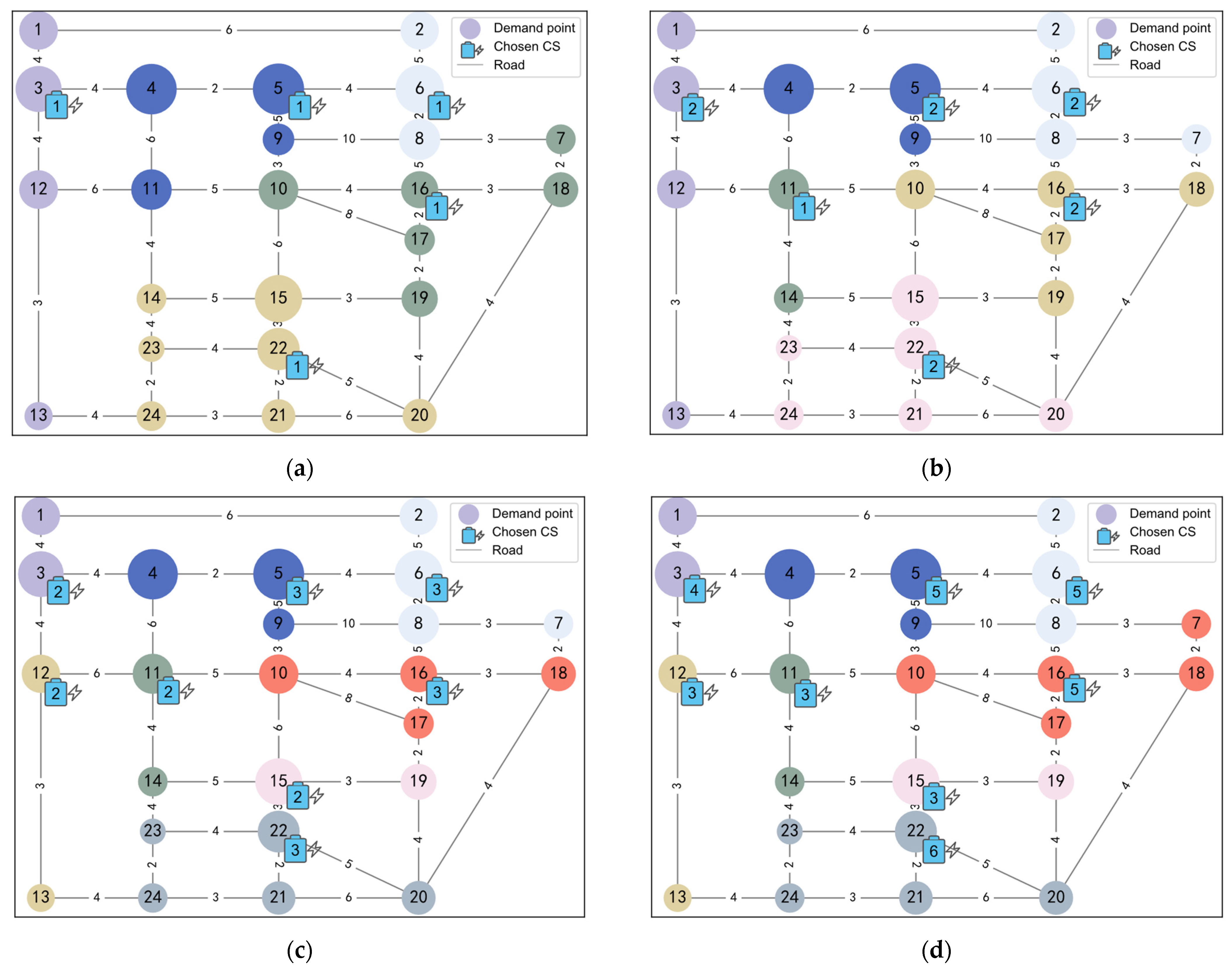
4.2. Layout Optimization Results

4.2.1. Location Optimization Results

Based on the above spatial-temporal distribution of charging demand, the optimal results of multistage layout for CSs are shown in Figure 5 and Figure 6. The preselected β was set as 1.2, whose selection method is shown in Section 4.3.1. In each stage, the whole road network is divided into several approximately uniform sub-networks whose centers are set with a CS in consideration of road length and charging demand, which can ensure more EVs can be charged in a relatively short distance and reduce the range anxiety of EV users. As time goes on, the numbers of CSs and FCPs increase and the average areas served by CSs become smaller because of the increasing charging demand at demand points. CSs in the same locations or as the relocation destination of other CSs become the centers of the sub-network from preceding stages to later stages for the adjustment of pairing the relationship between EV users and CSs, which demonstrates the effectiveness of the model and the rationality of the location optimization results.
The above layout characteristics of CSs in the sub-networks are fully reflected at all stages except for some seemingly abnormal phenomenon. In Figure 5d, not like in Figure 5c, some EVs at demand points do not go to the nearest CSs but a farther one, such as the EV at demand point 10, which goes to CS 11 for charging but not to CS 16. This sub-optimal phenomenon is mainly caused by two reasons; one is that the overload operation of the nearest CS and the new added charging demand will lead to another new built CS and higher cost, and the other reason is that the farther charging selection will decrease the total number of FCPs and the cost savings will cover the detour cost of the EV users.

4.2.2. Capacity Optimization Results

The capacity optimization results are also verified. The CS with more FCPs will cover more charging demand according to Figure 5. Take Figure 5e as an example, CS 3 equipped with 10 FCPs and CS 12 equipped with 6 FCPs both serve EVs of two demand points, but the charging demand served by CS 3 is bigger according to the sizes of nodes. With the increasing trajectories, the optimal total number of FCPs is increasing proportionally, which can satisfy the charging demand at various stages, as shown in Figure 6. The FCPs are scattered across several CSs but not concentrated at a CS to decrease the high detour cost of each EV user at early stages, which caused the intensive CS construction at early stages and relatively high early cost related to CSs, as shown in Figure 6. The above analysis demonstrates the optimization sizes of CSs are consistent with charging demand, both in amount and spatial distribution.

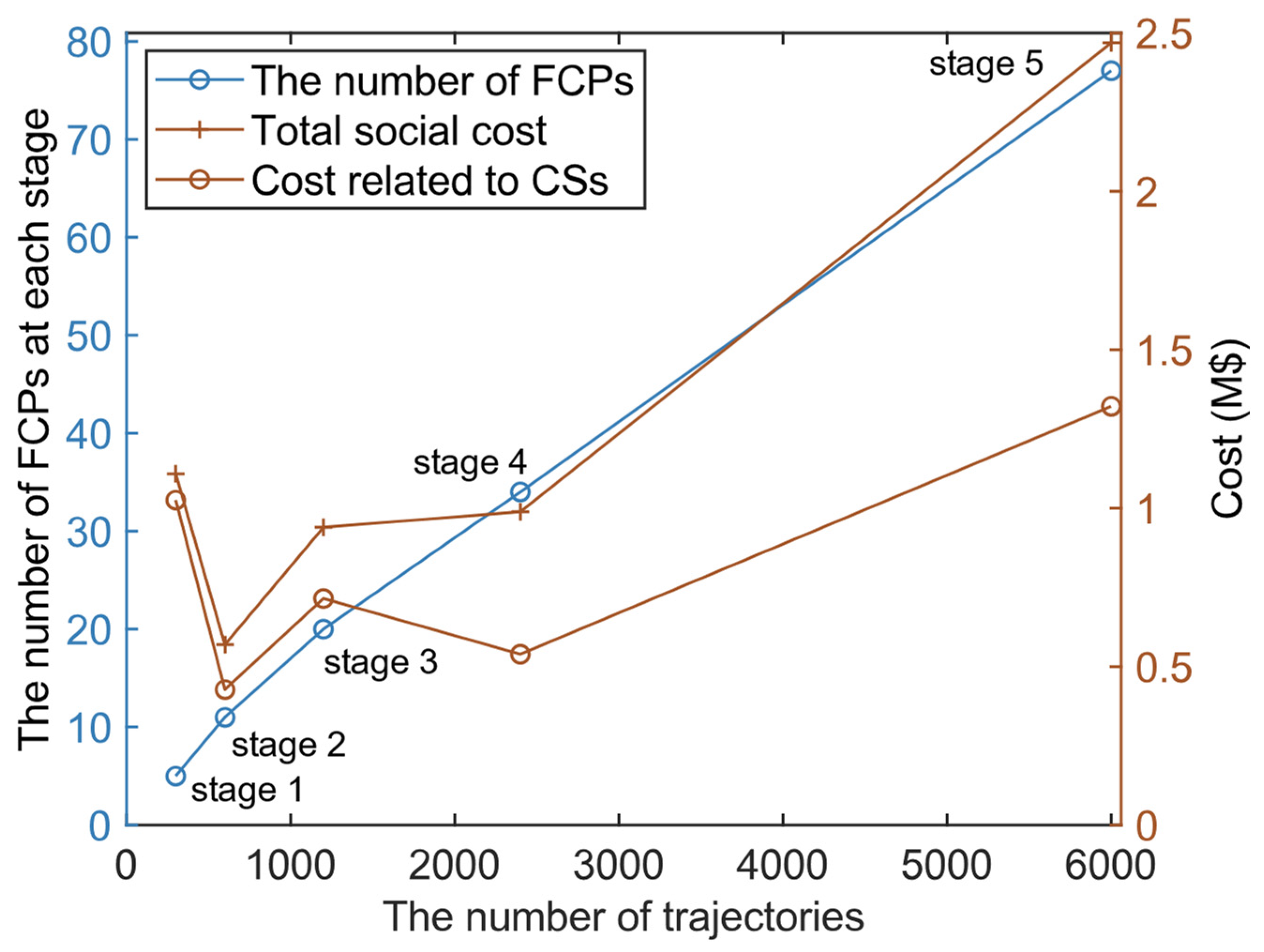
4.2.3. One-Time Strategy vs. Multistage Strategy

One-time optimization strategy means that CSs equipped with FCPs are built at the beginning aiming to satisfy the final charging demand in long-term planning. As Figure 5 and Table 2 show, the total numbers of CSs and FCPs in them are the same. Furthermore, the locations of CSs and the sizes of each CS at the last stage with the multistage strategy are the same as that with the one-time strategy, which means the final stage with the relatively larger number of EV trajectories has a great influence on the optimization results. Comparing to the one-time strategy, the multistage strategy can configure the numbers of CSs and FCPs, and even the locations of CSs flexibly at different stages, which leads to operating and maintenance cost savings. On the contrary, with the multistage strategy, the detour cost and η are larger because of the fewer charging infrastructures at all stages except the last one. However, the costs related to CSs and TSC drop sharply, respectively, by 13.72% and 8.79%, which shows higher economic viability and less waste from a global perspective.

4.3. Sensitivity Analysis

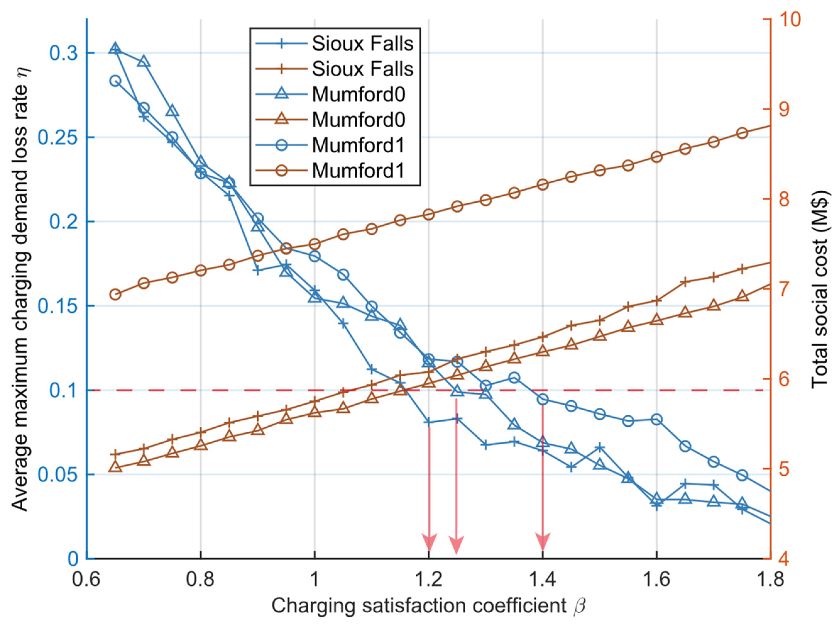
4.3.1. Sensitivity Analysis and the Selection of β

In this section, the TSC- η - β relationship has been studied by changing the preselected parameter β in MILP model spaced by 5%. Another two tests based on the Mumford 0 network (with 30 nodes and 90 lines) and Mumford 1 network (with 70 nodes and 210 lines) [17] have been added to prove the generality of the results.
In Figure 7, with the increasing of β , the optimal TSC increases almost linearly but the charging demand loss rate η decreases, almost following a negative exponential function, which indicates that the marginal benefit declines after a certain amount of investment. Some values of η increase with higher β and larger TSC, which were mainly caused by the unbalanced charging demand allocation and resource shortage in some CSs. These abnormal values would not influence the general trends of the curves.
In this paper, it is assumed that a loss rate of η is less than its maximum allowed demand loss, which is 10%. It is hard to know the selection standard from the decision maker’s perspective, and the maximum allowed loss rate can be adjusted accordingly in reality. When the maximum allowed demand loss rate is determined, we need to select the minimum value of β satisfying that demand loss, which is 10% in our paper, e.g., β = 1.2 for the Sioux Falls network, as the arrows in Figure 7 have shown. A lower value of β gives rise to a lower TSC, and the minimum value of β will be selected in satisfying the demand loss constraints (<10%).

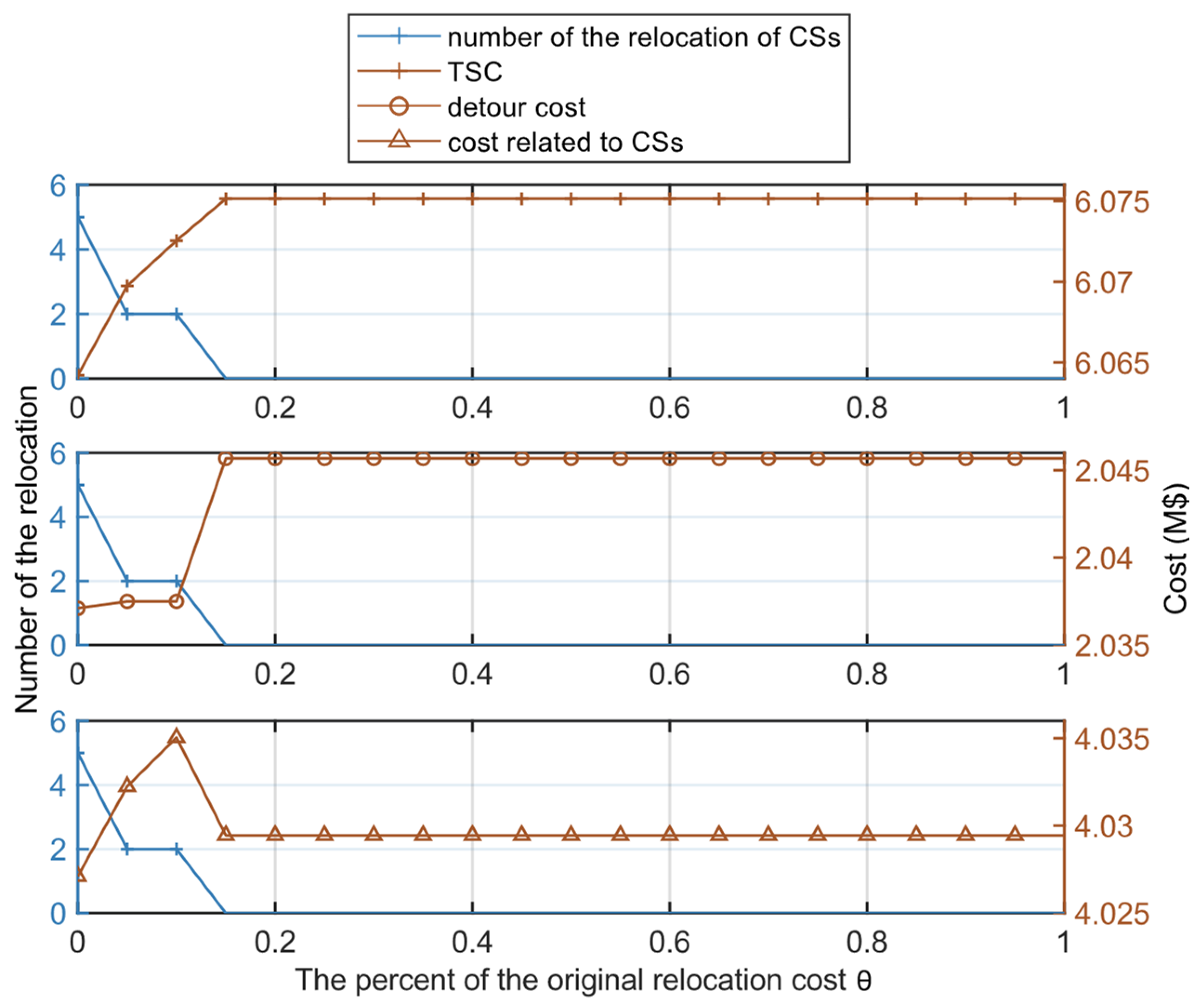
4.3.2. Sensitivity Analysis of the Relocation Cost

The relocation process did not appear in the layout optimization results, as shown in Figure 5. A sensitivity analysis of the relocation cost is designed, and the optimization results are as shown in Figure 8.
The θ is the indicator used to describe the reduction in the relocation cost. In Figure 7, when θ > 0.15 , the optimal TSC is always the same and the number of the relocation of CSs is zero, which means the economic benefit of relocation cannot cover the relocation cost. When θ = 0.15 , the TSC decreases with the cost decrease in detours and the cost increase related to CSs, which means the relocation strategy shortens the distance between EV users and CSs and leads to the economic benefit higher than the relocation cost. When θ = 0 , the cost related to CSs with relocation is lower than that without relocation, which indicates the relocation strategy can reduce the investment with the higher use ratio of FCPs. When the relocation cost is lower than a threshold, the lower the relocation cost, the more flexible the layout of CSs and the lower the TSC. Based on the above analysis, the relocation strategy can lead to a decrease in TSC when the relocation cost is relatively low compared to other costs.

4.3.3. Sensitivity Analysis of Road Network Scales

As a combinational optimization problem with NP-hard characteristics, when the urban road network scale becomes larger, the optimization will be difficult, especially in consideration of multiple dimensions and non-linear features in the model. Several road networks with different structures and scales have been selected to test the computational efficiency of the MILP model, as shown in Table 3. When the number of nodes is less than 224, the optimization time is less than 3 min with the optimization error controlled under 0.5%, which shows that the multistage layout optimization model has high optimization accuracy, especially for small and medium networks. The optimization time can also be accepted considering the low computational speed requirement for location layout problems. The optimization results also show that the TSC increases obviously with the increases of the road network scales, and higher power consumption of EV on the travel may be one of the key reasons.

5. Conclusions and Future Work

The layout of CSs needs to adapt to the rapid growth of EV charging demand both in terms of time and space. This paper proposed a multistage and dynamic layout optimization model for CS layout planning to minimize TSC considering the travelers’ dynamic behavior in a day, which can satisfy the charging demand at different stages more precisely. The model was constructed by using MILP, and different computational techniques such as piecewise linear (PWL) were applied to balance the calculation efficiency and precision. The charging satisfaction coefficient and M/M/S/K model of the queuing theory were introduced to decide the desirable number of FCPs. The layout effectiveness of the proposed model has been demonstrated by the optimization results of the numerical example, and the calculation efficiency and precision have been verified by the sensitivity analysis, especially for the small and medium networks. The main findings are concluded as follows:
  • The final stage with a relatively large number of EV trajectories has a great influence on the optimization results with both multistage strategy and one-time strategy. TSC with multistage optimization strategy can drop 8.79% from that with one-time optimization strategy in the case study, which can provide some meaningful suggestions for the long-term planning of EV CSs.
  • Charging service quality, relocation cost, and road network scales have a significant impact on the optimization results. Surplus supply of charging demand for the charging peak is necessary to decrease the charging demand loss caused by uneven EV arrivals.
For future work, the analysis of EV users’ behavior will be further refined to make the prediction of the spatial-temporal distribution of charging demand more accurate and reliable. This paper mainly focuses on the deployment problem of CSs from the perspective of transportation systems. Reference [28] provides an integrated modeling approach between a transportation system and power distribution system, inspiring us to strengthen the considerations of the distribution grid in our model, such as optimal power flow and the V2G problem.

Author Contributions

Conceptualization, F.C. and S.L.; methodology, F.C. and S.L.; software, F.C. and M.F.; validation, S.L., B.H., M.F. and F.C.; investigation, F.C.; resources, S.L. and B.H.; writing—original draft preparation, F.C.; writing—review and editing, S.L., B.H. and M.F.; visualization, M.F. and F.C.; supervision, S.L., B.H. and M.F.; project administration, S.L. All authors have read and agreed to the published version of the manuscript.

Funding

The author(s) disclosed the receipt of the following financial support for the research, authorship, and/or publication of this article: The work described in this paper has received funding from the Featured Creative Project of Higher Education Institution of Guangdong Province, China (NO.2021KTSCX001), in part by the Fundamental Research Funds for the Central Universities (NO.2020ZYGXZR087), and the State Key Laboratory of Rail Traffic Control and Safety (Contract No.RCS2021K008), Beijing Jiaotong University.

Data Availability Statement

The data of the road networks are available from the open databases: https://github.com/bstabler/TransportationNetworks (accessed on 1 September 2021). https://github.com/RenatoArbex/TransitNetworkDesign (accessed on 1 September 2021).

Acknowledgments

We would like to thank Fei Xue from Xi’an Jiaotong-Liverpool University for his generous support and useful discussions during the preparation of this paper.

Conflicts of Interest

The authors declare no conflict of interest.

Nomenclature

Abbreviations
CCSscandidate charging stations
CSscharging stations
EVelectric vehicles
FCPsfast charging piles
MILPmixed integer linear programming
PWLpiecewise linear method
SOCstate of charge
TSCtotal social cost
UFZurban functional zone
Indices
r trajectory from 1 to R
s point on the trajectory from 1 to S r
i demand point from 1 to N
t time interval from 1 to T
j candidate charging station from 1 to M
k planning stage from 1 to K
Parameters
R total number of trajectories
S r total number of points on trajectory r
N total number of demand points
T total number of time intervals
M total number of candidate charging stations
K total number of planning stages
l s r location of point s on trajectory r
t s r time of point s on trajectory r
S O C s r S O C of point s on trajectory r
P s r charging probability of point s on trajectory r
d s r shortest path distance from point s to the departure point on trajectory r
δ s r auxiliary probability of charging probability
V average EV speed
γ driving range per kilowatt-hour
C m rated capacity of EV battery
S O C ¯ / S O C _ upper/lower limit of charging
α control coefficient between the detour cost and cost related to CSs
β charging satisfaction coefficient
F i , j , t monetary cost from i to j in time interval t for an EV
F average hourly wage
d i , j shortest path distance from i to j
V i , j , t EV speed from i to j in time interval t
J E V , k detour cost of EV users at stage k
J C S , k cost related to CSs at stage k
J C S , j , k c s construction and relocation cost of CS j at stage k
J C S , j , k c p installation and relocation cost of FCPs in CS j at stage k
J C S , j , k c s , r / J C S , j , k c p , r operating cost of CS j /maintenance cost of FCPs in CS j
C c c s / C o c s / C r c s construction/operating/relocation cost of a CS
C c c p / C o c p / C r c p installation/maintenance/relocation cost of a FCP
P c charging rated power of FCPs
Δ T a time interval
G j , k upper limit of the number of FCPs caused by the land and the distribution grid
Variables
h s , i , t r =1 represents the point s on trajectory r is at demand point i in time interval t ; 0, otherwise
W i , t traffic flow at demand point i in time interval t
D i , t charging demand at demand point i in time interval t
x i , j , k =1 represents EVs at demand point i choose CCS j for charging; 0, otherwise
y j , k =1 represents CCS j is open at stage k ; 0, otherwise
z j , k number of FCPs installed in CCS j at stage k

Appendix A

This subsection will work as the supplementary of the M/M/S/K model [29], and the subscript of variables in Section 3.2 will be removed for concision. For example, ρ j , t , k will be replaced by ρ , which means the following discussion focuses on the specific CS and the specific time interval.
ρ s = ρ s
p 0 = { ( n = 0 s 1 ρ n n ! + ρ s ( 1 ρ s K m s + 1 ) s ! ( 1 ρ s ) ) 1 , ρ s 1 ( n = 0 s 1 ρ n n ! + ρ s s ! ( K m s + 1 ) ) 1 , ρ s = 1
p n = { ρ n n ! p 0 , 0 n < s ρ n s ! s n s p 0 ,   s n K m
η = p K m
In Formula (A1), s and ρ s represent the number of FCPs and the service strength of the CS, respectively. In formula (A2), K m represents the capacity of the CS, including charging and waiting spaces and n represents the number of EVs in the CS. p n represents the probability of n EV in CS, so p 0 represents the possibility that the CS is idle. η represents the charging demand loss rate because the EV with charging demand needs to leave the CS when all charging and waiting spaces have been occupied.

References

  1. Global EV Outlook 2020. Available online: https://www.iea.org/reports/global-ev-outlook-2020 (accessed on 12 November 2021).
  2. Palomino, A.; Parvania, M. Advanced charging infrastructure for enabling electrified transportation. Electr. J. 2019, 32, 21–26. [Google Scholar] [CrossRef]
  3. Pure Electric Vehicles Feel Charging Pinch on Highways during National Day Holidays. Available online: https://www.globaltimes.cn/page/202110/1235651.shtml (accessed on 10 October 2021).
  4. Zhang, L.; Brown, T.; Samuelsen, S. Evaluation of charging infrastructure requirements and operating costs for plug-in electric vehicles. J. Power Sources 2013, 240, 515–524. [Google Scholar] [CrossRef]
  5. Tian, Z.; Hou, W.; Gu, X.; Gu, F.; Yao, B. The location optimization of electric vehicle charging stations considering charging behavior. Simulation 2018, 94, 625–636. [Google Scholar] [CrossRef] [Green Version]
  6. Xiang, Y.; Jiang, Z.; Gu, C.; Teng, F.; Wei, X.; Wang, Y. Electric vehicle charging in smart grid: A spatial-temporal simulation method. Energy 2019, 189, 116221. [Google Scholar] [CrossRef]
  7. Xie, F.; Liu, C.; Li, S.; Lin, Z.; Huang, Y. Long-term strategic planning of inter-city fast charging infrastructure for battery electric vehicles. Transp. Res. Part E Logist. Transp. Rev. 2018, 109, 261–276. [Google Scholar] [CrossRef]
  8. Lin, Y.; Zhang, K.; Shen, Z.-J.M.; Ye, B.; Miao, L. Multistage large-scale charging station planning for electric buses considering transportation network and power grid. Transp. Res. Part C Emerg. Technol. 2019, 107, 423–443. [Google Scholar] [CrossRef]
  9. Li, S.; Huang, Y.; Mason, S.J. A multi-period optimization model for the deployment of public electric vehicle charging stations on network. Transp. Res. Part C Emerg. Technol. 2016, 65, 128–143. [Google Scholar] [CrossRef]
  10. Han, B.; Lu, S.; Xue, F.; Jiang, L.; Xu, X. Three-stage electric vehicle scheduling considering stakeholders economic inconsistency and battery degradation. IET Cyber-Phys. Syst. 2017, 2, 102–110. [Google Scholar] [CrossRef]
  11. Zhang, H.; Moura, S.J.; Hu, Z.; Song, Y. PEV Fast-Charging Station Siting and Sizing on Coupled Transportation and Power Networks. IEEE Trans. Smart Grid 2018, 9, 2595–2605. [Google Scholar] [CrossRef]
  12. He, S.Y.; Kuo, Y.-H.; Wu, D. Incorporating institutional and spatial factors in the selection of the optimal locations of public electric vehicle charging facilities: A case study of Beijing, China. Transp. Res. Part C Emerg. Technol. 2016, 67, 131–148. [Google Scholar] [CrossRef]
  13. Ji, Z.; Huang, X. Plug-in electric vehicle charging infrastructure deployment of China towards 2020: Policies, methodologies, and challenges. Renew. Sustain. Energy Rev. 2018, 90, 710–727. [Google Scholar] [CrossRef]
  14. Vazifeh, M.M.; Zhang, H.; Santi, P.; Ratti, C. Optimizing the deployment of electric vehicle charging stations using pervasive mobility data. Transp. Res. Part A Policy Pract. 2019, 121, 75–91. [Google Scholar] [CrossRef] [Green Version]
  15. Guo, F.; Yang, J.; Lu, J. The battery charging station location problem: Impact of users’ range anxiety and distance convenience. Transp. Res. Part E Logist. Transp. Rev. 2018, 114, 1–18. [Google Scholar] [CrossRef]
  16. Ghamami, M.; Zockaie, A.; Wang, J.; Miller, S.; Kavianipour, M.; Shojaie, M.; Fakhrmoosavi, F.; Hohnstadt, L.; Singh, L. Electric Vehicle Charger Placement Optimization in Michigan: Phase I-Highways; Technical Report; 2019. Available online: https://www.researchgate.net/publication/331963177_Electric_Vehicle_Charger_Placement_Optimization_in_Michigan_Phase_I_-Highways (accessed on 1 September 2021).
  17. Transportation Networks for Research Core Team. Transportation Networks for Research. Available online: https://github.com/bstabler/TransportationNetworks (accessed on 18 September 2021).
  18. Mu, Y.; Wu, J.; Jenkins, N.; Jia, H.; Wang, C. A Spatial–Temporal model for grid impact analysis of plug-in electric vehicles. Appl. Energy 2014, 114, 456–465. [Google Scholar] [CrossRef] [Green Version]
  19. Sun, S.; Yang, Q.; Yan, W. A Novel Markov-Based Temporal-SoC Analysis for Characterizing PEV Charging Demand. IEEE Trans. Ind. Inf. 2018, 14, 156–166. [Google Scholar] [CrossRef]
  20. Lu, S.; Han, B.; Xue, F.; Jiang, L.; Feng, X. Stochastic bidding strategy of electric vehicles and energy storage systems in uncertain reserve market. IET Renew. Power Gener. 2020. [Google Scholar] [CrossRef]
  21. Lyu, M.; Han, B.; Lu, S. Electric Vehicle Operation Scheduling Optimization Considering Electrochemical Characteristics of Li-Ion Batteries. In Proceedings of the 2020 35th Youth Academic Annual Conference of Chinese Association of Automation (YAC), Zhanjiang, China, 16–18 October 2020; 2020. [Google Scholar]
  22. Cormen, T.H.; Leiserson, C.E.; Rivest, R.L. Introduction to Algorithms; MIT Press: Cambridge, MA, USA, 2007. [Google Scholar]
  23. Lin, M.-H.; Carlsson, J.G.; Ge, D.; Shi, J.; Tsai, J.-F. A Review of Piecewise Linearization Methods. Math. Probl. Eng. 2013, 2013, 1–8. [Google Scholar] [CrossRef] [Green Version]
  24. Overcoming Barriers to Electric-Vehicle Deployment: Interim Report; National Academies Press: Washington, DC, USA, 2013; p. 18320. [CrossRef]
  25. Das, H.S.; Rahman, M.M.; Li, S.; Tan, C.W. Electric vehicles standards, charging infrastructure, and impact on grid integration: A technological review. Renew. Sustain. Energy Rev. 2020, 120, 109618. [Google Scholar] [CrossRef]
  26. Zhang, H.; Hu, Z.; Xu, Z.; Song, Y. An Integrated Planning Framework for Different Types of PEV Charging Facilities in Urban Area. IEEE Trans. Smart Grid 2016, 7, 2273–2284. [Google Scholar] [CrossRef]
  27. Public Transit Networks for Research. Transit Network Design Instances for Research. Available online: https://github.com/RenatoArbex/TransitNetworkDesign (accessed on 18 September 2021).
  28. Wei, W.; Wu, D.; Wu, Q.; Shafie-Khah, M.; Catalão, J.P.S. Interdependence between transportation system and power distribution system: A comprehensive review on models and applications. J. Mod. Power Syst. Clean Energy 2019, 7, 433–448. [Google Scholar] [CrossRef] [Green Version]
  29. Xiao, D.; An, S.; Cai, H.; Wang, J.; Cai, H. An optimization model for electric vehicle charging infrastructure planning considering queuing behavior with finite queue length. J. Energy Storage 2020, 29, 101317. [Google Scholar] [CrossRef]
Figure 1. The topology of Sioux Falls road network with 24 nodes and 38 edges. Each node (24 in total) represents the road crossing, which corresponds to an urban functional zone (UFZ), and each edge (38 in total), with a number indicating the road length (km), illustrates the bidirectional road. The numbers on the nodes represent the ID of road crossings.
Wevj 12 00243 g001
Figure 2. Flow chart of simulating spatial-temporal distributions of traffic flow and charging demand based on the Monte Carlo method.
Wevj 12 00243 g002
Figure 3. A two-layer layout optimization model of EV charging stations. TSC- η - β relationship can be acquired by changing the presumed parameter β in the MILP model in different loops, which can help determine the desirable value of β and corresponding optimal layout results.
Wevj 12 00243 g003
Figure 4. The spatial-temporal distribution of traffic flow and charging demand with 10,000 trajectories in a day. The data are the average of the demand points with the same kind of UFZs. It can be found that the traffic flow and charging demand fluctuate in one day. (a) The distribution of traffic flow; (b) the distribution of charging demand.
Wevj 12 00243 g004
Figure 5. The locations of optimal CSs at different stages based on the Sioux Falls road network. The chosen CSs at each stage are labeled by the number of FCPs in them. The size of each circular node represents the relative amount of EV charging demand at each demand point in a day. EVs at the demand points with the same color will go to the CS in the corresponding color area for charging. (a) Stage 1; (b) Stage 2; (c) Stage 3; (d) Stage 4; (e) Stage 5; (f) layout optimization results with a one-time strategy.
Wevj 12 00243 g005aWevj 12 00243 g005b
Figure 6. Optimization results based on the Sioux Falls road network.
Wevj 12 00243 g006
Figure 7. Optimal results with different charging satisfaction coefficient β. Maximum here stands for the maximum charging demand loss rate for a CS in different time intervals on a day, and average is for all CSs at all stages.
Wevj 12 00243 g007
Figure 8. Optimization results with different relocation costs.
Wevj 12 00243 g008
Table 1. Key parameters in the optimization model.
ParametersSymbolsValue
Construction cost of a new CS C c c s USD 163,000
Installation cost of a FCP C c c p USD 23,500
Relocation cost of a CS 1 C r c s USD 26,000
Relocation cost of a FCP C r c p USD 500
Average hourly wage F USD 8.2
EV battery capacity 2 C m 40 kW·h
Driving range per kilowatt-hour 2 γ 6.075 km/kW·h
Rated charging power of FPCs 2 P c 80 kW
Upper/lower limit of charging S O C ¯ ,   S O C ¯ 0.80, 0.20
1 The relocation cost consists of trenching, backfill, site restoration, power lines, labor and so on [24]. 2 The parameters related to EV come from vehicle model “Leaf” [25] and the other parameters come from [26].
Table 2. Comparison of the optimization results of the one-time optimization strategy and the multistage optimization strategy.
StrategyTotal Number of CSsTotal Number of FCPsDetour Cost (M$)Cost Related to CSs (M$)Total Social Cost (M$)η
One-time8771.98994.67036.66028.097%
Multistage8772.04564.02956.07510.012%
Variation00+2.80%−13.72%−8.79%+8.085%
Table 3. Computational efficiency of the MILP model for different network scales. All numerical examples have the same parameter settings as the case based on Sioux Falls.
NameNumber of NodesNumber of LinesAverage Road Length (km)Total Social Cost (M$)Optimization Time (s)Gap
Sioux Falls 124384.136.07511.200
Mumford 0 230904.475.86421.440
Mumford 1 2702104.587.737634.220
Mumford 2 21103854.708.5771164.010
Mumford 3 21274254.628.8478128.290
Berlin Friedrichshain 12245234.6011.217138.28<0.5%
1 The data comes from [17]. The average road length of the Berlin Fredrichshain network has been set artificially to match other networks for the lack of length data. 2 The data comes from [27].
Publisher’s Note: MDPI stays neutral with regard to jurisdictional claims in published maps and institutional affiliations.

