Analysing the Cost-Effectiveness of Charging Stations for Electric Vehicles in the U.K.’s Rural Areas

Abstract

While U.K. authorities have attempted to tailor measures to boost sales of electric vehicles (EVs) and support citizens through different schemes, the size and geographic coverage of the existing charging network are insufficient, which undermines electromobility promotion. There are 15,853 public charging points installed in the U.K. as of 3 August 2021, and the demands for public EV charging are rising. For rural areas, there is little support from local authorities or private companies. To identify how a charging station can be installed and work, this study researches existing charging stations nationwide. Generally, most Public Charging Stations (PCS) in rural areas have unsatisfactory cost-effectiveness due to their long payback period. This paper presents how many rural PCS are able to afford the cost in the first eight years. Based on the ever-increasing demands of the market, EV producers are switching their business strategies. Meanwhile, the rural areas may become urban with the same definition. When it comes to the analysis of cost-effectiveness, it is possible for the PCS to bring more elements into the calculation. For Capital Expenditure (CAPEX) and Operation Expenditure (OPEX), the unnecessary cost leaves more profit space, like the possibility of unplanned maintenance costs.

1. Introduction

Greenhouse gases, including carbon dioxide, mainly originate from the transportation sector [1]. It carries on growing as the key factor in the economy and quality of life index, though global climate change and warming brings a big challenge to the development of human civilisation [2,3]. To reduce transport emissions, many European countries have adopted policy measures for clean power to transport [2]. The U.K. authorities have attempted to tailor measures to boost sales of electric vehicles (EVs) and support citizens through different schemes, for example, the U.K. government offers customers incentives in investing the EVs supply equipment (EVSE) [2].

EVs can resolve the greenhouse emission issue and the fossil fuel scarcity problem [4]. EVs are more economically affordable and environmentally friendly [5] compared to internal combustion engine vehicles (ICEV). The US Department of Energy reports that EVs convert 77% of electrical energy to power at the wheels, which differs from fuel-based vehicles that convert approximately 12–30% of the energy stored in gasoline [6]. EVs impact local and regional electricity grids as well [7]. EVs bring a socioeconomic development opportunity for islands and remote locations due to the reduction of fuel imports [8].

In Norway, drivers are willing to purchase EVs due to their financial viability rather than their environmental conscience [9]. Goldin et al. [10] found that EV owners can save 40% of annual maintenance costs. There are no tailpipe emissions, which plays a central role in pollution emission reduction [5].

The U.K. government strongly supports EV owners for sustainable development [11]. The local authorities are required to meet the various travel needs of individual and commercial motorists [12]. Strutt and Parker [13] predicted that the electric car market has expanded rapidly in recent years. With increasing consumer demand, greater availability of vehicles and government support, the sales of EVs keep growing in many countries, especially in China and Europe, but in the United States they dropped in 2019 [6,14,15]. Based on the record for battery-electric and plug-in vehicles, ultralow or zero-emission cars account for 19% of all the U.K.’s additional cars in 2019 [16].

It can be predicted that the accessibility of charging stations positively influences the electric vehicle market [1,17]. A survey showed that 69% of respondents would be willing to buy EVs once there was a discernible charging infrastructure [1]. To supply EVs, companies are obliged to adapt relative infrastructure and increase charging stations [18].

Nevertheless, it is not enough for charging points to meet the electricity demands and attract customers [18]. Hosseini and Sarder [5] claim that fast-charging sites positively impact the public acceptance of EVs. It is a chicken-and-egg problem that cannot be separated. Insufficient provision of public charging infrastructure slows down the growth of the domestic electric vehicle market [12]. Moreover, the mass uptake of EVs has a major barrier, PCS. The policy of attracting companies to install charging stations aims to grow the acceptance of electric mobility [18].

EVs must tackle the current inadequate charging infrastructure [1]. For those potential future electric vehicle owners who experienced ‘range anxiety’, additional charging infrastructure can well address it and increase electric vehicle uptake [6].

In terms water destruction, waste discharge, and greenhouse gas (GHG) reduction, the electric vehicle charging station (EVCS) performs excellently [2]. As an energy provider, charging stations have fundamentally impacted the industry development of EVs, which can also raise the acceptance of electric mobility with its user-friendliness. Meanwhile, the U.K. authorities does accept that PCS play a significant role in encouraging and boosting the uptake of EVs [2]. Minimising the total distance travelled by EVs with the selected charging stations positively impacts the development of the EV market [18].

Thus, sufficient charging stations are supposed to be available for ever-increasing EV sales, enabling electric vehicle owners to conveniently charge their vehicles [9]. On the other hand, economic or technical measures can be taken to guide and control the charging behaviour of EVs [11].

The optimal charging station network expands outward from the urban city as its number of stations increases. Fortunately, the funding from the U.K. government for installation of PCS on residential streets in 2021 will be doubled to £10 million due to the government’s ambition to gradually stop diesel and petrol cars and to assist EV drivers to easily locate and use affordable, reliable charging points whether at home or on the road by opening up data [9]. The prevalence of EVs on the road is supposed to increase the attractiveness of starting an EV charging station business [19].

The size and geographic coverage of the existing charging network are insufficient, which undermines electromobility promotion [12]. Meanwhile, EV consumers complain that recharging an EV is less convenient than refuelling an internal combustion vehicle [18]. The principal barrier for electric cars is a lack of choice and availability [20].

The Office for Low Emission Vehicles (OLEV) supports businesses with the previous costs to purchase and install new workplace charging stations, according to the Workplace Charging Scheme (WCS). The U.K. government encourages and leverages private sector investment on building a self-sustaining PCS network. Moreover, incentives are also given to consumers in purchasing ULEV cars [2].

There are 15,853 public charging points installed in the U.K. as of 3 August 2021, and the demands for public EV charging are rising [19]. The number of EV charge points per 100 km of road has increased from 42 to 570 in the UK [21]. For rural areas, there is little support from local authorities and little commercial intervention [12,22]. Charging infrastructures must also be developed in locations around towns [1]. Longer journeys need a network of charging points [7]. Meeting the demand for charging facilities is one of the tasks for rural estates with visitor attractions [13]. Minimising the total distance travelled by EVs with the selected charging stations positively impacts the development of the EV market [5].

Installing and running charging infrastructure involve a lot of issues. Before planning a charging station, investors need to consider the charger model, communications required, the number of chargers installed and the install specifics in terms of cabling, fixings and foundations; traffic convenience, population density, location safety, and security [5]. In Europe, there are more than five distinct types of sockets and two types of charging cables with different charging speeds [18]. After installing a charging point, managers are required to consider its service level capability [5].

Section 3, Section 4 and Section 5 discuss distinct models and Section 6 takes advantage of former sections to analyse the cost-effectiveness of the models. Section 7 summarises what this paper developed and suggests further studies.

2. Literature Review

User-friendly and economical charging stations increase the acceptance of electric mobility [18]. Data show EVs have lower annual maintenance costs compared to traditional petrol and diesel vehicles [10]. The electric car market has expanded rapidly in recent years [13]. The development of EV markets has raised the interest of investors in the EV charging stations [2,19]. Charging stations enable EV drivers to travel far [21]. Studies have shown the current main types of chargers with statistical supports [23,24]. Furthermore, three levels of charger need to be installed according to the local demands to achieve high net profit [4]. The energy issues for islands and remote locations were considered in a previous study [8], with the energy consumption in charging stations estimated using machine learning and relative methods [6]. The site selection of PCS and how it influences users’ daily life was developed in [5].

Different types of charging strategies serve many groups of people and various businesses. Investing in rapid-charging infrastructure was researched in [2] by listing parameters and structure of cost and revenue in the U.K. The authors developed a business model for this kind of charging station. They suggested the only revenue for charging stations is selling electricity. Bibby [25] demonstrates that the definitions of urban and rural classify all regions in the U.K. Both rural and urban locations have different types, and the U.K. government releases a definite list for rural and urban locations. Municipalities have the majority of EVs on U.K. roads [16] and there is little uptake of EVs in rural areas according to data from previous years.

Due to EV users’ various charging behaviours, most EV owners prefer to recharge their cars at home [7,8,11,26]. Surveys show that a small portion of charging events occur in public charging points [20].

Both CAPEX and OPEX have been applied to the financial analysis of charging stations [2,27]. A few articles generally estimate the common payback periods for PCS. Typically, the reasonable payback time is more than three years and up to seven years [1].

The above studies have investigated the development of EVs and how charging stations work. The majority of charge point-related details have been referred to, including calculating cost and revenue. Those studies have been reviewed in this project before analysis. There is a research gap for rural PCS, especially their cost-effectiveness.

This paper analyses the cost-effectiveness of installing and running a PCS network in rural areas. Compared to the PCS in the urban city, there are few advantages in investing in rural PCS, considering the differences between PCS in cities and rural areas [26]. Based on the parameters of charging infrastructure and data on EVs in the U.K., this paper forecasts electricity demands and calculates their payback periods, including making suggestions on increasing cost-effectiveness. Furthermore, the mathematical models in this paper can be swiftly applied in different situation with corresponding data.

3. Data and Methodology

The methodology of this project was developed for multidimensional analysis of the financial elements of charging stations in the U.K., especially in rural areas. Suitable business models have been developed for public charging infrastructures in suburban regions due to the distinct functions of charging stations in city centres and these areas. Listing the advantages and drawbacks of those business models contributes to the selection of the right one.

After confirming the corresponding business model, this paper analyses its cost and revenue. As for the cost of the charging station, it can be calculated through capital expenditure (CAPEX) and operational expenditure (OPEX). The CAPEX is required before operations begin and the OPEX is related to the operation and maintenance of chargers [2]. The parameters of CAPEX and OPEX mainly refer to information released by the U.K. government.

Before calculating the revenue of public charging stations, the equation requires electricity demands. It is less likely to search the definite electricity data due to the charging events varying a lot. Moreover, there are few surveys on how frequently EV drivers use their cars and into their various charging behaviours. Thus, this paper uses the average electric car range and the average electricity consumption per 100 miles. The relationship between EVs number and electricity demands is represented below in the equation. It is vital to identify the percentage of charging events happening in public charging stations since this project mainly focuses on them. The equation is as follows:

E_d = E_v × 193 × 0.3 × 0.05

(1)

In this equation, E_d is electricity demands for public charging points. E_v is the number of electric vehicles.

Yurday [28] reports the average electric car range is 193 miles in the U.K. at the beginning of 2021, but the range in summer is different from that of winter. To reduce the margin of error, this paper has calculated it in years. EV manufacturers should include the numbers for the whole year. For different EV types, the number of kilowatt hours (kWh) an electric car uses is not the same. An electric car is supposed to use approximately 30 kWh every 100 miles, which can be used in calculating electricity consumption [29]. Muzi [20] points out that 5% of charging events happen in public charging points, including chargers on the street, in car parks and along road corridors.

4. Urban and Rural Area Definition

An explicit classification method is required in analysing PCS in the U.K.’s rural areas. Rural-urban definition for small-area geographies (RUC) is an essential fundamental principle in this paper. The grid of hectare cells is a standard for the identification of settlements within RUC [25]. Classifying rural and urban areas requires a few steps due to profiles and files. Two files are mentioned in this paper, (RUC2011) and (RUC2001), which are the updates of the past two decades.

As is shown in Figure 1, this flow chart demonstrates how the government classifies areas. Several elements should be considered, including former files, residence, and population, etc. RUC has another dimension, which involves context in the physical settlement. A two-level typology of rural areas is shown below:

In Figure 2, sparseness represents the local density, and both rural and urban areas have been generally split into two parts. Each part still contains three settlement types.

On the other hand, urban is the same in segregation, but the branches in sparseness are different. A conurbation consists of a large area with grown and joined towns, usually near a city. According to their scale, conurbations can be separated into major and minor.

The map in Figure 3 clearly displays urban and rural areas with colours. Regions in urban areas are marked in four different shades of grey. It is evident that rural areas dominate the U.K., and play a vital role in connecting cities.

In this project, rural areas consist of three types: ‘largely rural’, ‘mainly rural’, and ‘urban with significant rural’. After selecting the corresponding codes, according to

Table 1. Local authority districts ranked by rural and hub-town (rural-related) populations from the 2011 rural-urban classification [30].

LAD15CD	LADNM	RUC11	Total Rural Population 2011	Total Hub Town Population 2011	Total Rural and Hub-Town (Rural-Related) Population 2011	Percentage of the Total Population 2011
E06000052	Cornwall	Mainly rural (rural including hub towns ≥ 80%)	326,682	115,347	442,029	83.0
E06000054	Wiltshire	Largely rural (rural including hub towns 50–79%)	223,719	93,566	317,285	67.4
E06000047	County Durham	Largely rural (rural including hub towns 50–79%)	231,417	81,151	312,568	60.9
E06000051	Shropshire	Largely rural (rural including hub towns 50–79%)	175,469	53,688	229,157	74.9
E06000057	Northumberland	Largely rural (rural including hub towns 50–79%)	145,096	78,801	223,897	70.8
E06000011	East Riding of Yorkshire	Largely rural (rural including hub towns 50–79%)	146,674	53,794	200,468	60.0
E06000056	Central Bedfordshire	Largely rural (rural including hub towns 50–79%)	100,272	48,234	148,506	58.4

, in

Table 2. Plug-in cars and light goods vehicles licensed at the end of quarter by upper and lower tier local authority 2, United Kingdom from 2011 Q4 (Part) [31].

ONS LA Code (April-2019)	Region/Local Authority (April-2019)	2021 Q1	2020 Q4	2020 Q3	2020 Q2
K02000001	United Kingdom	468,949	413,642	355,963	300,981
K03000001	Great Britain	463,374	408,854	351,806	297,354
E92000001	England	418,204	369,260	317,869	268,371
E12000001	North East	6773	5959	5411	4666
E06000047	County Durham	1313	1191	1080	930
E06000005	Darlington	362	318	294	244
E06000001	Hartlepool	143	129	124	109
E06000002	Middlesbrough	160	137	118	86
E06000057	Northumberland	1319	1188	1085	936
E06000003	Redcar and Cleveland	200	172	155	135
E06000004	Stockton-on-Tees	473	394	328	274
E11000007	Tyne and Wear (Met County)	2799	2426	2222	1947

, we collected licensed EVs numbers of 138 rural areas. The 138 groups of data are the basis for the cost-effectiveness analysis. After distinguishing where the rural areas are, this paper seeks business strategies for PCS. As presented in Table 2, the lines in Bold are rural area data. In the U.K., London is the municipality with the highest number of battery-electric and plug-in hybrid cars [16].

5. Business Model Selection

Before selecting business models, this paper researched charging behaviours among EV consumers. Approximately 50% to 80% of all charging events happen at home, based on the average number of charging events [7]. Fifteen to twenty-five percent of charging events occur at work [7,26], and the remaining 5% of charging events happen in a PCS, including on-street city charging, chargers in car parks, and fast charging along road corridors [7,20].

In Figure 4, home charge dominates the charging events. Serradilla et al. [2] suggest that credible business models are developed, which will bring more private investment to the PCS market. The companies lack motivation due to insufficient innovative business models [18]. Thus, a suitable business model for PCS in rural areas is required in this project. This section lists several popular business models for EVCSs, analysed and compared in a multidimensional way.

Three ways were introduced to build a charging station business profitably and sustainably [32].

Table 3. Three EVCS business models [32].

Model Type	Characteristic	Best for
1. Install EVCSs to attract tenants	Provide chargers free to business owners, tenants and visitors Attract EV owners Also bill for EVCSs	Property owners and managers of multiunit complexes Commercial real estate owners Landlords who lease space to other businesses, including retail stores and office space Retail store owner Hotel and hospitality property owners
2. Showcase the commitment to conservation and sustainability	Offer EVCSs for free to customers, guests or tenants in your housing complex, hotel, or retail and entertainment centre. Gain revenue by increasing visitors to retail centre or charging higher rent	Smart business owners Hotel owner Landlord of complex; retail and entertainment owner
3. Recover energy cost	Earn grants and subsidies Incentives (reducing costs) Promote your brand as an ecoconscious company (Optional) charge customer directly	Company (business)

presents three models’ characteristics and what groups of people they are suitable for.

Both Model 1 and Model 2 have other purposes before being installed. In other words, investors do not expect to be profitable through charging customers or users. They find the business opportunities from attracting EV owners, rather than charging them. Those who have additional or unplanned space where they can install EVCSs prefer Model 1 because EVCSs bring more functions to their buildings and properties. The revenue from EVCSs are just a tiny part of their business, but they indeed play an essential role in attracting more people and gaining popularity.

The EVCS in Model 2 is similar to parking lots for specific areas or property. As a facility, EVCSs serve those who live or work in the area for business purposes. The hotels, complexes, and centres with EVCSs have a higher value. Thus, landlords or business people could set a higher rent than those that do not have EVCSs.

As for Model 3, it takes advantage of the local sustainability programs. The incentives include funding them with a tax credit [32]. It is a win-win for the government and companies to stimulate the EV market and promote their ecoconscious brands.

In conclusion, the three proposed models [32] take advantage of the potential value of EVCSs. However, they do not suit PCS in rural areas because the cost of installation and running is unaffordable for private investors.

In

Table 4. Five EV charging business models [33].

Model Types	Targets	Features	Advantages
1. Regional fast charging networks	(Major) private and public enterprises	Require long-term partnership and internal resources More competitive in markets and brands	Rejuvenate old premises Boost new business
2. Local small business initiatives	For towns, cities and tourist attractions Cooperative small business group Restricted by regulations or policy	Accessible to new electric vehicle drivers Fit for mid-sized towns	Maximise revenue from peak seasonal traffic
3. Commercial EV charging	Business with off-street parking Retailers, shopping centres, hotels Turnkey solution (CPMS; RFID card; Apps)	Low risk and low investment	Attract new and high-value customer Improve customer satisfaction Become more competitive as a ‘green company’
4. E-fleets and enterprises	Large corporations	Fleet managers switch to electric vehicles Government incentives	Employee-friendly Low maintenance costs
5. Municipalities and sustainable e-mobility	Local councils	Driven by low emission vehicle programs Local incentives Provide facilities to other firms	Benefit to tourism and communications

, five different business models for EVCSs are presented [33], which massively consider most of the situations in regions, firms, and local authorities. There are some initial conditions in Models 1 and 3, like off-street parking or sufficient internal resources. Managers and investors recognise EVCSs as tools rather than as a core business element in Model 1. For corporations whose employees are EV owners, installing an EVCS is a necessary and cost-effective way to meet charging demands. Governments are encouraging enterprises, firms, and councils to invest in EVCSs with running programs or incentives. As for those who plan to invest in EVCSs in rural areas, Model 2 could be considered. Rural areas contain towns, urban fringe, and villages where population density is relatively low. The study showed less than 0.1% EV uptake in rural areas, which means those regions are less likely to attract investors due to the risk in installation and management of EVCSs. However, rural areas do not just connect regions but attract tourists with their visitor attractions. Thus, Model 2 can bring business opportunities to EVCSs in those places with lower risk and higher ROI compared to other models. Furthermore, the other business models can be applied in this project since the advantages somehow fit the conditions of rural charging stations. For example, if there is an available space for parking, companies or landlords can also apply commercial EV charging. A reliable fast-charging network is required in the PCS business, which involves a long-term partnership and resources from companies or governments. Judging from the business models mentioned above, the installation of PCS vary by region, EV uptake, and local policy, etc. When this paper sought a business model for rural PCS, it found no unique model that can be perfectly applied. Investors of small business groups may install more than one PCS in rural areas with a fast charge network, commercially billing customers and users.

The many business models for EVCS cannot all be analysed in this paper. This paper discusses the drawbacks of four classical business models. The levels of revenue can be seen in

Table 5. Business models for commercial EV charging [34].

Model Types	Targets	Features
1. Loss leader model	Free for EV drivers (attract and retain customers) Grow brand loyalty Boost on-site revenue	Liability for installing and running EVCS Not friendly to rapid charging stations
2. Operational cost or total cost recovery	Charge EV drivers to fill the operational cost Alternatively, pay back hardware and installation cost with additional margin Suitable for rapid charging stations	Less attractive for EV owners (compared with Model 1) No extra profit
3. Profit making	Higher fee charging on EV owners For those places where there is no alternative charger for drivers	Less attractive for EV owners (Possible) reputational damage due to unfair price
4. Fully funded	Offer to a business (no capital or operational cost) Requires a long-term view	No pricing initiative

. In Models 1 to 3, a regulation can be designed so that the higher price of an EVCS, the less attractive it is. Thus, the price for EV owners is a deciding factor in commercial EV charging.

As for price setting, it depends on how much profit investors plan to achieve. Dynamic spike pricing (DSP) policy was introduced, which was proposed to reduce the charging cost of EVs [11]. The competitiveness in a region impacts the development of charging stations, while the current charging price is generally fixed or related to the different periods [17]. Business investors who cannot be fully funded by governments or charging infrastructure providers are more likely to be concerned about its cost-effectiveness.

In this section, the business models play a central role in deciding how businesses allocate costs and make a profit for rural PCS. In the following sections, we analyse the expenses and revenues of PCS in rural areas.

6. Results and Discussions

To analyse cost-effectiveness, this paper refers to several parameters in the cost and revenue of PCS. The cost of EVCSs include construction, maintenance, and operating costs [5]. In terms of costs, there are two terms—capital Expenditure (CAPEX) and operational Expenditure (OPEX).

6.1. CAPEX

In this paper, CAPEX contains five models as shown in Figure 5, and the details of the models are elaborated in

Table 6. Summary of CAPEX parameters [2].

Element	Definition	Parameter
Charger purchase and delivery	Multi standard chargers Delivery to local storage facility	350 GBP per socket
Installation management	Managing all on-site work (survey, permission, building warrants, labour etc.) Working with stakeholders (site operators, landlord, DNO cost)	N/A
DNO power connections	A new power connection from the chargers to the local electricity distribution Power, install specifics (cable length, transformer, fix etc.) In the U.K., the single DNO distribute electricity from the grid to each business in that region	15(26%) of RCN (1000 to 20,000 GBP) 7500 GBP (15% site rent)
Site preparation	All civil and electrical engineering work Charger installation (excavation; cabling, plinths, feeder pillars switch gear metering equipment, bay marking, signage etc.)	N/A
Commissioning	Delivering EVSE from storage facility to local site Power connection, limited communication test, function and safety checks	N/A

.

As is listed in Table 6, some of the models have parameters that vary by country or area. For management, site preparation, and commission, there is no relative statistical support. The U.K. government announced that it contributes 350 GBP per charger towards workplace EV charging stations. Moreover, a general commercial PCS installation costs around 1000–1500 GBP plus VAT (1118–1675 EUR) in total. Expected investments are 36,500 GBP per charger in CAPEX, and rising to £42,000 with a new power connection.

Figure 6 shows that the majority of CAPEX is the cost of purchasing, delivering, and installing chargers. About 60–80% of the cost of a public EV charger is the installation [35]. The way investors distribute funds to those models depends on the type of charger, site, and budget, etc. Even if the total CAPEX has a parameter, its branch data are still necessary for the following calculation because some of the parameters are related to OPEX. For instance, maintenance cost and unplanned maintenance cost are according to the cost of charger purchase and delivery. Furthermore, installing a grid-connected charging station is not just related expenditure but also construction permits, local unity and time [36].

6.2. OPEX

OPEX consists of five models just like CAPEX.

Table 7. Summary of OPEX parameter [2].

Element	Definition
Electricity cost	The cost of energy The amount of electricity was recorded by a meter
Site rent	Paid by EMSP (to site operator)
Back office running costs	Managing chargers User-related costs (registration; RFID cards; online user account capabilities; customer support service) Software (providing; updating; further development)
Maintenance cost	Routine checks, call-out arrangements establishment
Unplanned maintenance cost	Unexpected events (vandalism; nonwarranty part)

explains the models in Figure 7 with parameters and resources. Unlike Table 6, the models in Table 7 have relative parameters which are related to CAPEX.

In 2020, the U.K. electricity price per kWh according to the Department for Business, Energy and Industrial Strategy was 0.172 GBP. Tenants need to pay £50,000 or above per year. However, the charging stations in rural areas are less likely to reach this kind of site rent. In this project, the site rent will be £1000 (per year) because tenants do not have to rent so much land.

6.3. Revenue

Electricity sales are a unique way that charging points can raise revenue. The daily charger usage costs contribute to 80% of EV charging [34]. Thus, the electricity demands, cost of electricity, and price for EV drivers are required parameters in calculations. These parameters change dynamically. For instance, the electricity purchase cost rises 5.2% annually [2]. The price for EV drivers to recharge will rise simultaneously. Thus, this project assumes that the gap between electricity cost and the price is the same.

A total annual profit of around 200 GBP is achievable when “selling” electricity at a profit of 0.04 GBP per kWh [37]. But the price of recharging varies by region, type of charger, car brand, etc. Pod Point rapid chargers cost 23 p/kWh at Lidl and 24 p/kWh at Tesco [38]. According to Tesla, EV owners are charged at 26.4 p per kWh [38].

Current types of charging stations include Level 1, Level 2, and DC fast chargers (DCFC) [24]. There are three types of charger in the U.K.—slow chargers, fast chargers, and rapid chargers. The features and parameters of these chargers are displayed in

Table 8. Types of chargers [23].

Charger Types	Features	Parameter
Slow charger	The basic charger Allow to charge overnight	A maximum current draw of 3 kW
Fast chargers	Double the rate of charge Decrease ‘fully charged’ time	A current draw up to 7 kW
Rapid chargers	80% of capacity in just half an hour	A current draw up to 120 kW

.

The parameters are related to how much it costs per charger per year. There is little literature about the relationship between EV owners and the number of chargers in one charging station. This paper assumes that one PCS in the rural area typically provides two chargers. The CAPEX and OPEX can be estimated in the following section.

To summarise, the electricity purchase cost is 0.172 GBP per kWh, and sales price is 0.264 GBP per kWh, which is applied in cost-effective analysis combined with electricity demands.

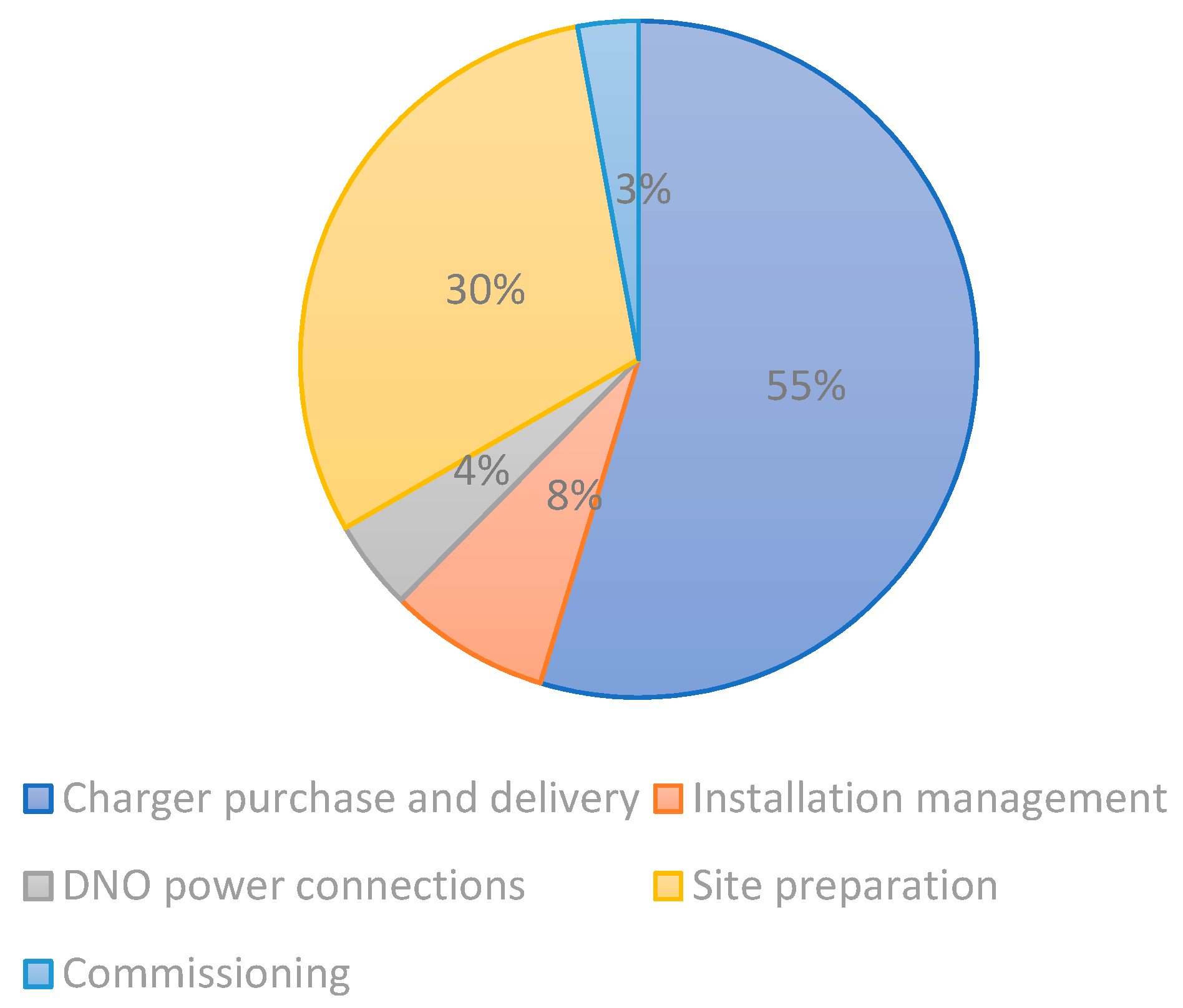
The parameters and equation in Section 3 and Section 6 will be applied in this part. Based on Table 7, this project firstly calculates the CAPEX of the charging station.

As is assumed in the end of Section 6.3, there are two chargers in this station. Thus, the amount of CAPEX can be easily calculated (

Table 9. CAPEX of a charging station in the rural area.

	Elements	Parameter
CAPEX	Chargers number	2
	Charger purchase and delivery	350 GBP × 2
	Installation management
	Distribution network operator (DNO) Power connections	150 GBP
	Site preparation
	Commissioning

). This number is less likely to influence the following analysis once a PCS has been installed.

6.4. Electricity Usage Forecast

OPEX is highly related to the number of existing EVs according to Equation (1). The unique variable in

Table 10. OPEX of a charging station in the rural area (annual).

	Elements	Parameter
OPEX	Electricity cost	0.172 GBP × Ed
	Site rent	1000 GBP
	Back office running costs	250 GBP × 2
	Maintenance cost	0.03 GBP × 700
	Unplanned maintenance costs	0.04 GBP × 700

is Ed. To demonstrate the method for dealing with OPEX, this project predicts the electricity demands of County Durham in

Table 11. The forecast of electricity consumption in County Durham.

	2020 Q2	2020 Q3	2020 Q4	2021 Q1	2021 Q2	2021 Q3	2021 Q4	2022 Q1
Ev	930	1080	1191	1313	1435	1562	1656	1764
Ed	-	-	-	3801.135	4154.325	4521.99	4794.12	5106.78

.

Before calculating Ed, this paper applies linear programming in an Ev forecast. Judging from the statistical information in Table 2, the number of licensed vehicles experienced an increasing trend.

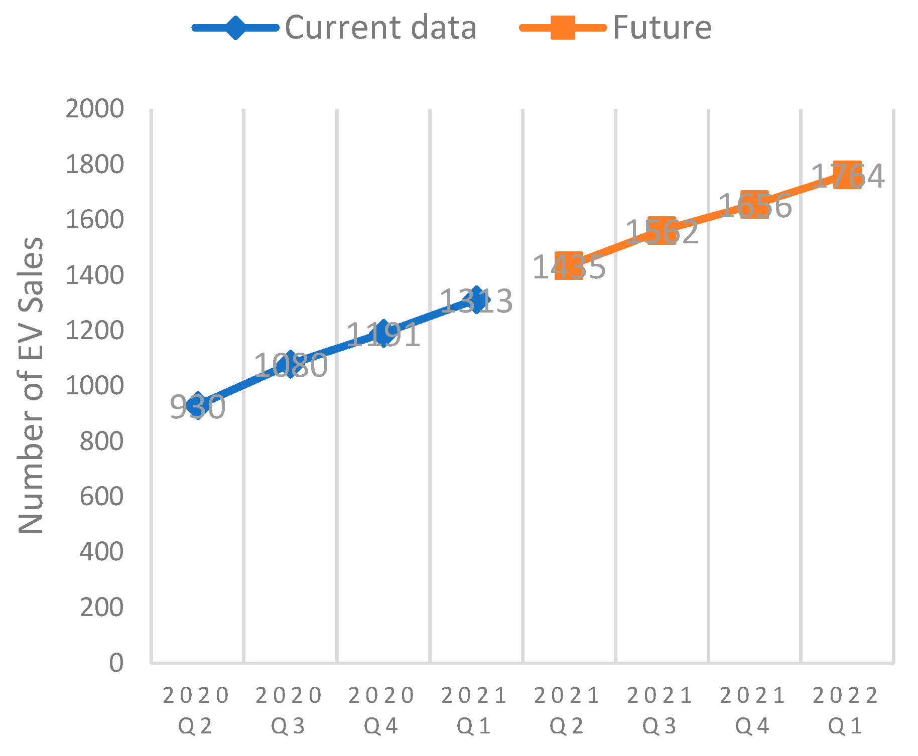
To accurately forecast electricity demands in the next four quarters, this paper uses ten groups of EVs, which have not been shown in Table 11, with the help of the ‘FORECAST’ function in Excel. The numbers in the second line are presented. The reason that this paper predicts future EVs is to estimate payback time. Through this method, future data can be addressed. The trend of Ed and Ev can be seen in Figure 8 and Figure 9.

However, not all groups of data have a constant growing tendency. For example, Figure 10 shows that the number of licensed vehicles in the Isles of Scilly increases and decreases during this period, but it moderately begins to rise from 2020. So, this project chooses to make the prediction based on the latest data from quarter 1 2020 to quarter 1 2021.

The more recent data is shown in the first quarter of 2021. This paper selects the first quarter in the following years to represent the corresponding Ev of this year. The selected data are printed in yellow in

Table 12. Selection of forecasted data per quarter.

Region/Local Authority (April-2019)	2021 Q1	Q2	Q3	Q4	2022 Q1	Q2	Q3	Q4	2023 Q1	Q2	Q3	Q4	2024 Q1
County Durham	1313	1435	1562	1656	1764	1879	1994	2111	2224	2338	2448	2559	2671
Northumberland	1319	1436	1564	1655	1758	1867	1979	2094	2205	2316	2422	2528	2636
Redcar and Cleveland	200	220	241	262	283	303	323	347	368	389	410	431	452
Cheshire West and Chester	1555	1687	1791	1906	2026	2150	2273	2398	2519	2640	2758	2878	2999
	Year 1				Year 2				Year 3				Year 4

. After refining and simplifying the tables, this section finally collects Ev in

Table 13. Selection of E_v data per year.

Region/Local Authority (April-2019)	Year 1	Year 2	Year 3	Year 4	Year 5	Year 6	Year 7	Year 8
County Durham	1313	1764	2224	2671	3127	3580	4032	4486
Northumberland	1319	1758	2205	2636	3078	3517	3953	4393
Redcar and Cleveland	200	283	368	452	536	620	704	789
Cheshire West and Chester	1555	2026	2519	2999	3480	3965	4446	4930
Allerdale	194	310	425	541	656	771	887	1002
Barrow-in-Furness	97	123	149	175	201	228	254	280
Carlisle	272	433	589	746	904	1060	1218	1375
Copeland	132	176	220	263	307	351	394	438
Eden	190	288	384	479	576	671	767	863
South Lakeland	516	729	936	1142	1351	1557	1765	1973

.

Combining Equation (1) and Table 12, Ed in the rural areas can be calculated, as is shown in Table 13. This paper predicts the data of the next thirty-two quarters because the further a prediction is made, the more error it has. This project selected eight numbers from those thirty-two prediction numbers to prevent the error from influencing the accuracy and dependency in the following calculations.

After calculating the Ed, all columns in

Table 14. Selection of E_d data (kWh).

Region/Local Authority (April-2019)	Year 1	Year 2	Year 3	Year 4	Year 5	Year 6	Year 7	Year 8
County Durham	3801	5107	6439	7734	9052	10,365	11,672	12,986
Northumberland	3819	5088	6384	7631	8910	10,181	11,445	12,718
Redcar and Cleveland	579	819	1064	1308	1551	1796	2039	2283
Cheshire West and Chester	4502	5866	7291	8681	10,075	11,478	12,872	14,271
Allerdale	562	898	1230	1565	1899	2233	2568	2902
Barrow-in-Furness	281	355	432	507	583	659	735	810
Carlisle	787	1255	1704	2158	2617	3070	3526	3981
Copeland	382	509	638	762	889	1016	1142	1268
Eden	550	834	1112	1387	1667	1943	2221	2499
South Lakeland	1494	2110	2709	3305	3910	4509	5109	5711

have a definite value. This paper displays some of the data that are used in the following research.

6.5. Revenue Calculation

Filling the column with values completes Table 10. Then, the OPEX of the next eight years have their own value.

Table 15. OPEX analysis of County Durham (Year 1).

	Elements	Parameter (£)
OPEX	Electricity cost	654
	Site rent	1000
	Back office running costs	500
	Maintenance cost	21
	Unplanned maintenance costs	28
	Total	2203

lists the detailed data of OPEX in County Durham in the first year.

Based on the results, in the next few years in County Durham, investors do not need to spend money on CAPEX, but the OPEX will change as time goes by due to the dynamic variable Ed.

The revenue also needs the data of Ed. Ed plus price for EV drivers equals total revenue. The net revenue can then be calculated by minimising the CAPEX and OPEX.

As is shown in

Table 16. Cost and revenue of PCS in County Durham.

		Year 1	Year 2	Year 3	Year 4	Year 5	Year 6	Year 7	Year 8
Cost	CAPEX	−£7300	0	0	0	0	0	0	0
	OPEX	−£2203	−£2427	−£2657	−£2879	−£3106	−£3332	−£3557	−£3783
	Accumulative	−£9503	−£11,930	−£14,587	−£17,466	−£20,572	−£23,904	−£27,461	−£31,244
Revenue		£1003	£1348	£1700	£2042	£2390	£2736	£3081	£3428
	Accumulative	£1003	£2351	£4051	£6093	£8483	£11,219	£14,300	£17728
Net		−£8500	−£9579	−£10,536	−£11.373	−£12.089	−£12,685	−£13,161	−£13,516

, for the whole eight years the net income for the PCS is negative, meaning no profit was made from this charging point during this period.

To observe dynamic changes, the data were inputted into line graphs.

As shown in Figure 11a, the cost has a more dramatic increase trend compared to that of revenue. The Figure 11b shows how net revenue change in years. The revenue cannot cover its cost, and the gap between cost and revenue is growing, which means this PCS cannot make a profit if investors do not adjust in time. The actual cost-effectiveness of setting up charging infrastructures is very poor. It is necessary to identify the reasons why there is no rising tendency in net revenue.

6.6. Reasons and Solutions

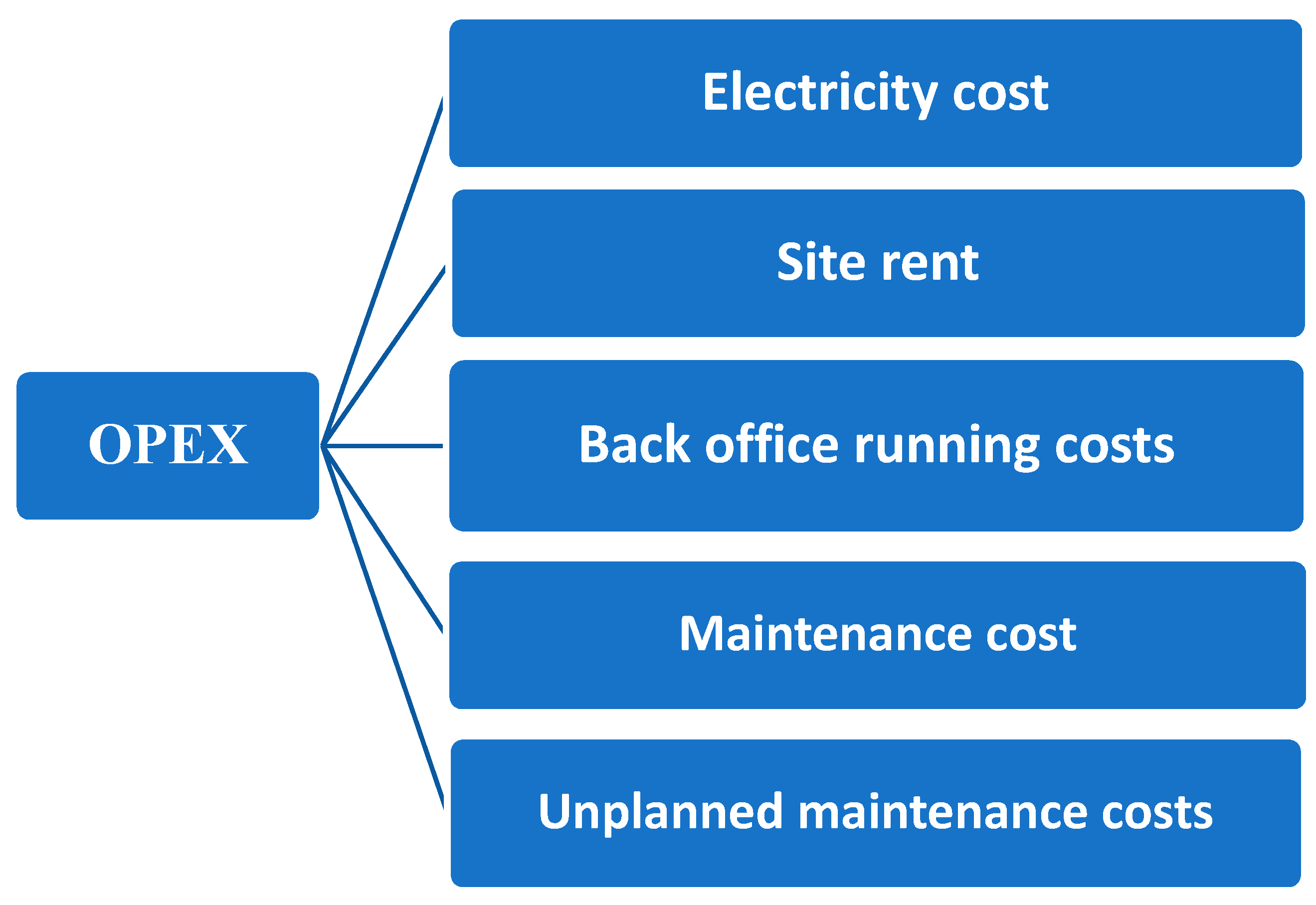
OPEX plays a vital role in the increase of total cost once installation has been completed. Thus, the factors that influence the speed of increase feed into OPEX. The factors are listed below.

The unchangeable factors in

Table 17. Influential factors.

	Elements	Influence or Not	Changeable Factors
OPEX	Electricity cost	No
	Site rent	No
	Back office running costs	Yes	Number of chargers
	Maintenance cost	Yes	Number of chargers
	Unplanned maintenance costs	Yes	Number of chargers

are ‘Site rent’ and ‘Electricity cost’. There is no change in site rent, except that other bodies can fund PCS. Furthermore, businesses are unable to boost Ed—the unique variable in electricity cost. The cost of electricity purchase is a national standard measured by the government.

The last three elements are related to the number of chargers. Therefore, reducing the number of chargers is an available method to slow down the speed of total OPEX. Moreover, CAPEX declines at the same time. After changing one factor, this paper analyses the effectiveness of one charger in County Durham.

Table 18. Summary of improved OPEX of County Durham (Year 1).

	Elements	Parameter (GBP)
OPEX	Electricity cost	654
	Site rent	1000
	Back office running costs	250
	Maintenance cost	10.5
	Unplanned maintenance costs	14
	Total	1928.5

lists the details of novel OPEX, and Table 18 updates its cost and revenue in County Durham. However, the net revenue remains the same, negative.

During these eight years, the total cost in PCS with one charger still outnumbers that of revenue. Nevertheless, there is an apparent minimal decrease trend closing to the end of the year. It means the speed of increase in revenue exceeds that of cost. With the ever-decreasing gap between cost and revenue, charging stations in County Durham will profit in the following years.

It is a fact that can be seen in

Table 19. Cost and revenue of PCS in County Durham (one charger) in GBP.

		Year 1	Year 2	Year 3	Year 4	Year 5	Year 6	Year 7	Year 8
Cost	CAPEX	−£3650	0	0	0	0	0	0	0
	OPEX	−£1928	−£2427	−£2382	−£2605	−£2831	−£3057	−£3282	−£3508
	Accumulative	−£5578	−£8006	−£10,388	−£12,993	−£15,824	−£18,881	−£22,163	−£25,671
Revenue		£1003	£1348	£1700	£2042	£2390	£2736	£3081	£3428
	Accumulative	£1003	£2351	£4051	£6093	£8483	£11,219	£14,300	£17,728
Net		−£4575	−£5655	−£6337	−£6900	−£7341	−£7662	−£7863	−£7943

and Figure 12 that the decreasing trend gradually slows down.

It seems that the investment in rural PCS is likely to pay back after eight years. However, the lifespan of payback is long for investors who cannot afford this tremendous loss. It is essential to seek other methods of boosting net revenue.

As we mentioned before, profit is related to electricity demands.

The decision variables used in our model are as follows:

x	Year
$f\left(x\right)$	OPEX in this year
$f^{\prime }\left(x\right)$	Revenue in this year
$f^{″}\left(x\right)$	Annual net revenue

$$f\left(x\right)=1274.5+0.172\times E_{dx}\hspace{1em}x\in \left[1,8\right]$$

(2)

$$f^{\prime }\left(x\right)=0.264\times E_{dx}\hspace{1em}x\in \left[1,8\right]$$

(3)

Both Equations (2) and (3) share the same variable—E_d. The total amount of site rent, back office running costs, maintenance costs, and unplanned maintenance costs is 1274.50 GBP. Equation (3) minus Equation (2) equals annual revenue.

$$f^{″}\left(x\right)=0.092\times E_{dx}-1274.5\hspace{1em}x\in \left[1,8\right]$$

(4)

When f″(x) is a positive value, there is no loss in that year. If f″(x) remains negative, the net revenue will not be positive anymore.

The minimal number of chargers is one. Currently, the cost cannot be cut by reducing the number of chargers. Fortunately, there is one last parameter that has not been changed—the profit gap. If investors plan to make a profit as soon as possible, they can bill EV drivers more in electricity price.

For instance, this paper assumes that investors increase rates from 0.264 GBP per kWh to 0.50 GBP per kWh. It can easily be predicted that the trend of total revenue is sharper than before.

As is shown in

Table 20. Cost and revenue of PCS in County Durham (one charger and higher price) in GBP.

		Year 1	Year 2	Year 3	Year 4	Year 5	Year 6	Year 7	Year 8
Cost	CAPEX	£3650	0	0	0	0	0	0	0
	OPEX	£1928	£2427	£2382	£2605	£2831	£3057	£3282	£3508
	Accumulative	£5578	£8006	£10,388	£12,993	£15,824	£18,881	£22,163	£25,671
Revenue		£1901	£2554	£3220	£3867	£4526	£5183	£5836	£6493
	Accumulative	£1901	£3557	£6776	£10,643	£15,169	£20,352	£26,187	£32,680
Net		−£3678	−£3552	−£2714	−£1452	£243	£2368	£4922	£7907

, the PCS in County Durham starts to make a profit in year 6. Figure 13 shows that the total revenue covers the total cost and rises dramatically in the following years.

Based on the data in

Table 21. Annual net revenue of County Durham (one charger and 0.005 GBP/kWh) in GBP.

	Year 1	Year 2	Year 3	Year 4	Year 5	Year 6	Year 7	Year 8
Annual cost	£5578	£2427	£2382	£2605	£2831	£3057	£3282	£3508
Annual revenue	£1901	£2554	£3220	£3867	£4526	£5183	5836	£6493
Annual net revenue	−£3678	£126	£838	£1262	£1694	£2125	£2554	£2985

, the internal rate of return (IRR) can be calculated in Excel. The IRR in

Table 22. IRR analysis of County Durham (one charger) in GBP.

Sales Price	Annual Net Revenue								IRR
	Year 1	Year 2	Year 3	Year 4	Year 5	Year 6	Year 7	Year 8
£0.3	−£4438	−£895	−£450	−£285	−£116	£52	£219	£388	−32%
£0.4	−£4058	−£385	£194	£489	£789	£1089	£1387	£1686	5%
£0.5	−£3678	£126	£838	£1262	£1694	£2125	£2554	£2985	27%
£0.6	−£3298	£637	£1482	£2036	£2600	£3162	£3721	£4283	49%

is 27%, which means it will earn a 27% compound annual growth rate. The IRR is positively related to revenue, once the CAPEX is confirmed. There is no standard for PCS to have a certain IRR. The businesses can opt to adjust parameters and compare them to select the highest one.

The different levels of sales price correspond to different levels of IRR shown in Table 22. The IRR shares positive relationships with the sales price. The precondition is that the electricity demands do not impact sales price. The private investors can compare the IRR of different rural PCS and go for the most profitable one.

The sales price of 0.50 GBP per kWh cannot guarantee that all rural PCS are able to pay back in these eight years. Equation (4) can be applied to calculate how many electricity demands it needs. The first parameter in Equation (4) switches to 0.328.

When f″(x) exceeds 0, it requires E_d to achieve 3770.71. It means the annual revenue of this PCS can cover the OPEX when its electricity demands reach 3770 during these eight years. There is no standard or reference timeline for investors to pay back the fund. This section suggests two ways to shorten the payback period. One is reducing the cost where possible and another one is raising the price for EV drivers. As for cost-saving, it has a bottom line since the necessity of management and hardware. The conditions of PCS are the basement of future development and running. On the contrary, there is no maximum for charging electricity, but, the high price of recharging for EV drivers is likely to negatively impact electricity demands, public reputation, and EV development, etc. Even though the price for EV drivers doubled and it ignores the CAPEX, there are still 30 rural regions that cannot make any profit during these eight years due to insufficient electricity demands. The 30 rural regions include North Devon, Scarborough, Rutland, Redcar and Cleveland, the Isles of Scilly and others.

Figure 14 shows that the regions with insufficient E_d account for 22% of PCS in all rural regions. Predictably, those PCS with not enough E_d will suffer from consistent losses over eight years.

Meanwhile, the PCS with sufficient E_d may still make losses for many years. Compared with those regions with insufficient E_d, they just have a capability of recovering costs.

This paper highly recommends that investors consider cost-reduction first because rising prices may raise complaints among EV drivers. If there is little effect in making profits, then the business begins to manage the price according to the revenue they want to produce.

6.7. Payback Period

There are 138 groups of data regarding current vehicle numbers and predictions. It is difficult to calculate them one by one but this paper calculates how much electricity demand they need in those eight years to cover the cost. In other words, the latest payback period is eight years.

With the assistance of Equations (2) and (3), this paper accumulates those eight groups of data to list an equation of total cost.

The decision variables used in our model are as follows:

x	Year
$F$	Total OPEX of 8 years
F′	Total revenue of 8 years

$$F={\displaystyle \sum }_{x=1}^{8}1274.5+0.172\times E_{dx}$$

(5)

$$F^{\prime }={\displaystyle \sum }_{x=1}^{8}0.5\times E_{dx}$$

(6)

$$F^{\prime }-F=3650$$

When the gap between F and F′ is 3650–CAPEX, the PCS eventually covers all the costs with sufficient revenue. Then this equation could be:

$$0.328\times {\displaystyle \sum }_{x=1}^8{E}_{dx}-\mathrm{10,196}=3650$$

(7)

After simplifying Equation (7), the results should be the integer:

$${\displaystyle \sum }_{\mathrm{x}=1}^8{E}_{dx}=\mathrm{42,213}$$

This point represents that the total cost of PCS equals that of total revenue. After calculating the amount of Ed, this project accumulates 138 groups of Ed to select those regions whose payback times are less than 8 years.

Forty-six regions can reach this line.

As shown in Figure 15, one-third of PCS in rural areas can pay back what they invest from 2021 to 2028, according to the sequences of total electricity demands. Those regions include Wiltshire, Glasgow City, Northumberland, and Central Bedfordshire, etc. The eight years’ payback period is a bottom line in this project. Spirit (n.d.) suggests that the payback period is typically five to eight years [39]. If these rural PCS are unable to reach this bottom line, the risk of it is high for investors. The cost-effectiveness of most investments in rural PCS is relatively low.

6.8. Summary

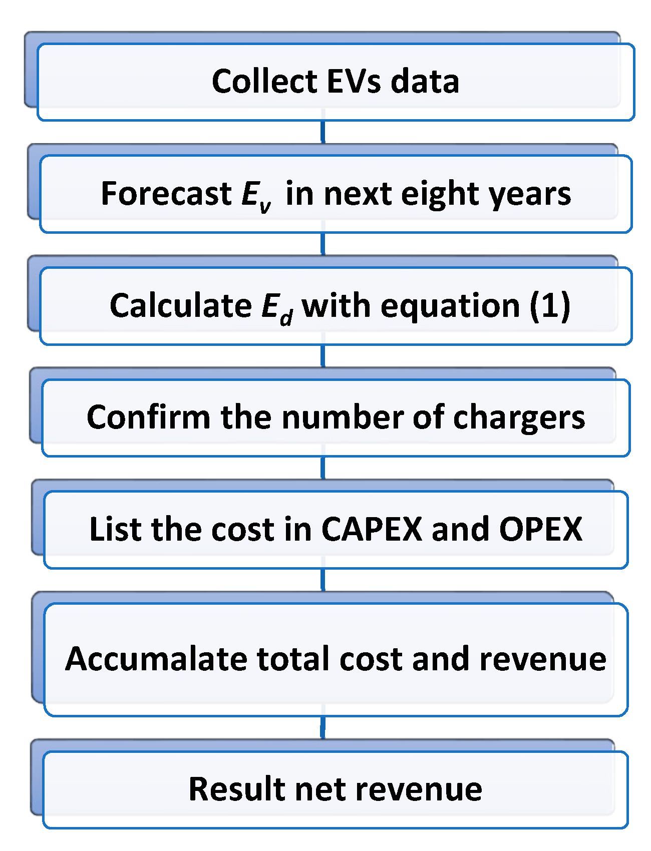
In this chapter, the parameters and methodology mentioned are applied. The calculation of Ed is elaborated in Section 3, but the prediction of Ev is completed in this section. The U.K. government’s data of licensed EVs strongly supports the prediction in this project. Enough statistical support can make the forecast more accurate. Mostly Ev experienced a moderate increase from 2011 to 2020, and fluctuations were seen in a few regions. Linear programming is a reasonable choice because the regulation can be easily spotted through the trends inside. However, the prediction is a mathematical result that cannot symbolise the authentic statistic. Based on the average car range, average electricity consumption per kilometre as well as the predicted Ev directly contribute to the Ed data from 2022 to 2028. The equations in this model are highly relative. Due to the closing relationship among equations, the results are more accurate and dependable with low error. Moreover, the cost-effectiveness analysis process is displayed in the flow chart below.

Through the process in Figure 16, net revenue can be calculated step by step. After calculating OPEX each year, this project has to add CAPEX in the first year and accumulate one by one. In other words, the total cost of a particular year contains CAPEX and all previous OPEX. The way of accumulating revenue is the same. Then, the total accumulated cost in that year minus that of revenue equals to current net revenue. The net revenue results in the tables mean how much net revenue the PCS gains or loses that year. If this result turns the negative number into a positive number, it means that this PCS starts to make a profit. However, the results show that there is no profit. The elements that influence the changes in net revenue have been identified in this project. Thus, two parts can be adjusted by investors. Figure 17 displays how this project works in case the net revenue remains negative during this period. Firstly, a dramatic decrease occurs in net revenue, meaning the revenue of PCS cannot cover its cost every year. On the contrary, the net revenue starts to climb, representing that the revenue of PCS is able to cover its annual cost, even if it is negative. This process can help investors gradually boost the revenue of PCS. Reducing the number of chargers to the minimum can cut the CAPEX and basement of OPEX, which directly decreases the total cost of PCS. However, it can slow down the growth rate of the total cost.

If there is a slight improvement in profit-making, it is reasonable for the business to speed up the growth rate of total revenue by raising the price. The rising price for EV drivers may bring other issues to PCS. As is suggested in Figure 16, the price could be changed more than once. So, investors have opportunities to change the price depending on the facts. For example, managers can slightly adjust the price at the beginning. Based on the evaluation of the growth rate in net revenue, another price adjustment could be considered. Before investing in PCS in rural areas, the business could estimate the revenue in the following years. This project gives an accessible model for evaluation. It is available for businesses to forecast their financial situation with this model. For managers running their PCS, the model can help them predict how many years they need to pay back, what they invest in or how much they can raise the electricity price. Meanwhile, for investors or companies who plan to install a PCS in rural areas, this analysis process references how many chargers they need, what a reasonable price is, and the possible payback period. Using line charts in this model shows the trend and compares cost and revenue in a one-time line. For example, the point where the total cost meets total revenue represents when this PCS turns loss into net profit. A gap exists after putting two lines into one chart: the value of net revenue. This paper uses two colours, blue and orange, to distinguish them. If an orange line is on top of the blue one, the PCS will make a profit.

This project assumes the same conditions—charger numbers, CAPEX, special electricity price. Once the charger number is confirmed, the only variable is Ed, as presented in Equation (7).

So long as this model presumes the latest payback time is eight years, the minimal total electricity demands of a PCS comes out. This number could be called the ‘electricity demands threshold’. In other words, if its total electricity demands reach this ‘threshold’, the PCS will pay back before 2028.

Investors can adjust this threshold. For instance, if businesses plan to pay back investments in five years, it changes the eight into five based on the Equations (5) and (6):

x	Year
$F_1$	Total OPEX of 5 years
${F_1}^{\prime }$	Total revenue of 5 years

$$F_1={\displaystyle \sum }_{x=1}^{5}1274.5+0.172\times E_{dx}$$

(8)

$${F_1}^{\prime }={\displaystyle \sum }_{x=1}^{5}0.5\times E_{dx}$$

(9)

$${F_1}^{\prime }-F_1=3650$$

The other parameters remain the same. The gap between Equations (8) and (9) equals the value of CAPEX. However, this ‘threshold’ cannot be changed by random. The lower the ‘threshold’ is, the less likely the charging stations can pay back their investments. Moreover, the purpose of the ‘threshold’ is to examine whether the PCS pays back in time.

Even though this model improves the cost and price, most rural PCS are less likely to gain any net profit before 2028.

7. Conclusions

This chapter aims to summarise all the results given in the whole paper and discuss the limitations and further research.

As listed in Figure 18, the content structure concludes the main tasks done in the project. Firstly, the environmental issues are threatening people, and the transport sector has to be responsible for air pollution, global warming and resource shortages, etc. Governments and authorities, therefore, encourage EVs as an alternative to traditional cars. Due to ever-expanding global EV markets, more charging stations are required to serve EV drivers and meet their electricity demands.

Installing a public charging point involves many incentives, from policy to management. To identify how a charging station is installed and works, this project researches existing charging stations nationwide. Although the charger types, charging speed, and cables varied by region, the design concept of the charging infrastructure is the same. The many charging points are suitable for different groups of EV drivers due to their various charging behaviours.

After completing all the preparation tasks, this project has all the critical data and tools. It lists cost and revenue step by step. The data collected were processed with linear programming to forecast quarterly EV numbers from 2021 to 2028, with County Durham used as an example. The first groups of net revenue show no profit over the period. The case of County Durham exposes the intrinsic problems.

After identifying the problems, this paper aimed to identify reasons and provide solutions. According to the calculation processes, two elements can help investors prevent the losses. Furthermore, after addressing issues with those two elements—charger number and sales price—we showed they have a logical relationship, as presented in a flow chart.

Generally, most PCS in rural areas have unsatisfactory cost-effectiveness due to their long payback period. This paper reveals how many rural PCS are able to afford the cost in the first eight years.

It is a dependable reference for businesses, investors, or companies to evaluate the cost-effectiveness of installing charging stations for EVs. Meanwhile, this paper suggests a brand new way of gaining cost-effectiveness for those who experience a negative trend in net revenue.

According to the results of this paper, managing a PCS plays a supporting role in installation and operations. A well-managed PCS with high cost-effectiveness not only benefits local EVs users, but also travellers. This study has flexibility in its calculations. Based on the results of this study, managers are able to select a rational payback period for their PCS with sufficient data of local EVs. Moreover, cost-control can be applied here by listing related CAPEX and OPEX. Automation and localised renewable energy sources for PCS like solar, wind, hydrokinetic could help standalone charging stations, especially those in the rural areas, to increase their cost-effectiveness.

7.1. Limitations

The parameters and variables in those equations have some limitations. The number of E_v forecasts vastly exceeds its sample number, which may cause unexpected errors among predictions of later years. Since E_d directly corresponds to E_v, the error will be added to the whole calculation process. Moreover, the average car range has dynamic changes, which impacts the speed of revenue growth rate.

As aforementioned, the profit gap between sales and electricity consumption remains the same as revenue directly involves E_d. Further, the relationship between the sales price and E_d is less likely to be expressed in the equation. If investors seek more profit by raising prices dramatically, they may suffer from decreasing sales due to negative reputation.

In fact, before installing a PCS in a certain place, investors need to confirm how many chargers a PCS should have based on local population or EV uptakes. There is little literature material in researching the relationship between charger number and local EV drivers. PCS do not just serve the people in the region as visitors and travellers who pass by may recharge their cars as well. Therefore, the 5% share of public charging events is not accurate in rural areas.

7.2. Further Research

The current literature briefly mentions the chicken-and-egg relationship between EVs and charging infrastructure. To what extent they influence each other is unknown, despite the complicity in modelling and constraints. The recharging issues cannot be discussed separately because the charger types and charging speed were standardised by EV manufacturers. Based on the demands of the market, EV producers are switching their business strategies. As the providers, charging stations have to take action to cater to EV markets. The inherent risk is an inevitable factor for private investors, businesses, and companies. The U.K. government is concerned about the whole EV industry. Incentives and policy encourage manufacturers as well as consumers. Meanwhile, the rural areas may become urban. The research on charging points in rural areas has to consider these regulation changes and urban classifications.

When it comes to the analysis of cost-effectiveness, it is possible to bring more elements into the calculation. For the CAPEX and OPEX, the unnecessary cost leaves more profit space, like the possibility of unplanned maintenance costs. In conclusion, the analysis needs more references and more dimensions in order to have a more comprehensive business model.