Context-Based Energy Disaggregation in Smart Homes

Abstract

In this paper, we address the problem of energy conservation and optimization in residential environments by providing users with useful information to solicit a change in consumption behavior. Taking care to highly limit the costs of installation and management, our work proposes a Non-Intrusive Load Monitoring (NILM) approach, which consists of disaggregating the whole-house power consumption into the individual portions associated to each device. State of the art NILM algorithms need monitoring data sampled at high frequency, thus requiring high costs for data collection and management. In this paper, we propose an NILM approach that relaxes the requirements on monitoring data since it uses total active power measurements gathered at low frequency (about 1 Hz). The proposed approach is based on the use of Factorial Hidden Markov Models (FHMM) in conjunction with context information related to the user presence in the house and the hourly utilization of appliances. Through a set of tests, we investigated how the use of these additional context-awareness features could improve disaggregation results with respect to the basic FHMM algorithm. The tests have been performed by using Tracebase, an open dataset made of data gathered from real home environments.

1. Introduction

Achieving greater energy efficiency through ICT has become an increasingly relevant research topic in the last decade. With the steady rise in consumption and the decreasing availability of energy resources, a remarkable slowing down in energy wasting, especially through the widespread adoption of energy saving solutions, is increasingly targeted.

It is expected that proper use of ICT (e.g., sensing, processing and actuation capabilities) would facilitate the achievement of this objective, in both domestic and industrial domains. The private home domain especially absorbs a non-negligible percentage of the energy demand. Indeed, domestic consumptions represent approximately one third of the whole energy usage in the European Union [1] as well as in the United States [2].

Several studies on domestic consumption habits [3,4], have shown that often users are not aware of how much energy is consumed by the devices they use. It has been recognized [5] that this may impair the understanding and adoption of energy saving behaviors. In other words, if the user were informed about how much a specific device affects total consumption, he might change his behavior in order to save energy as well as money.

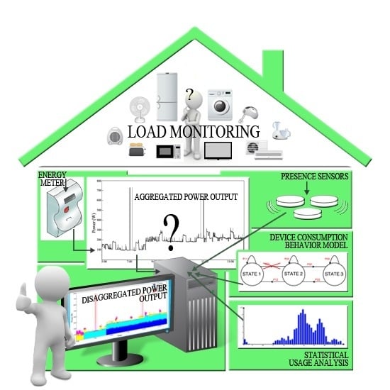
Hence, in this context, the introduction of Load Monitoring techniques, which support the continuous monitoring of electricity consumption and the consequent analysis of measured data, can also help in providing end-users with information and suggestions for improving their consumption behavior.

Load monitoring techniques can be grouped into three categories:

• Non-Intrusive Load Monitoring (NILM) [6]: NILM refers to a family of techniques whose purpose is to derive the power consumption of a specific device from the whole-house consumption profile.
• Hardware-based sub-metering: this technique is based on the deployment of a distributed system of low-cost metering devices (i.e., smart plugs attached onto household appliances) connected through a wireless and/or wired network infrastructure to a data collection module.
• Adoption of smart appliances: this approach relies on the use of household appliances enhanced with sensing, processing and communication capabilities that can remotely be controlled and configured.

Although the adoption of smart appliances would facilitate the user in implementing cost and energy actions, this approach is not likely to be put in place in the short term. Moreover, only a subset of devices are usually available as “smart appliances”, such as TVs, dishwashers, and ovens.

On the other side, smart plugs can be attached to almost any type of device. However, this approach can be resource demanding since a fine grained monitoring would require the use of a relevant number of smart plugs. In addition to the required financial commitment, the physical deployment might not be easy for fixed appliances (i.e., washing machine, dishwasher, refrigerator, etc.) or the user may be bothered by the obligation to constantly attach a smart plug to every portable device (i.e., hair dryer, phone charger, laptop, etc.).

On the other hand, NILM approaches which are based on whole-house consumption information can be easily deployed by leveraging existing and widely adopted smart meters. Several NILM algorithms have been proposed in literature [7] to disaggregate the output of smart meters. Most of them need monitoring data sampled at high frequency (at least 1 GHz frequency). In real-world scenarios, this assumption may be resource demanding whether the computation is performed locally in a Home Energy Management System (where data storage and processing resource-intensive tasks are performed) or in a remote server (since a high amount of data has to be transferred).

In this paper, we propose an NILM approach that relaxes the requirements on monitoring data since it uses total active power measurements gathered at low frequency (about 1 Hz). On one hand, this design choice has the advantage of allowing the use of low-cost metering devices. On the other hand, low-frequency measurements contain less information useful for load disaggregation than high frequency ones. To cope with this issue, in this paper, we enhance state of the art disaggregation approaches based on Factorial Hidden Markov Models (FHMM) [8] with the use of context information, i.e., information that can be gathered by home sensors on relevant events in the domestic environment to improve the accuracy of the disaggregation algorithm.

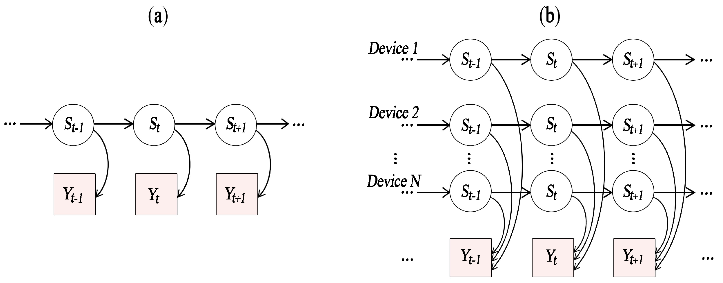
Our context-based energy disaggregation approach uses probabilistic models representing the appliances consumption behavior. More specifically, we adopted the additive Factorial Hidden Markov Model (FHMM) [9], where the observed variables represent the aggregated power consumption profile, while the hidden variables represent the states of appliances. Context information (namely user consumption patterns and users presence in a room) is exploited to vary the state transition probabilities of device models in order to improve the accuracy of results.

Moreover, the proposed approach has been tested using data gathered from real home environments and made available as an open dataset by the Technische Universität Darmstadt (i.e., Tracebase [10]). In our opinion, this choice may be scientifically relevant since it eases the comparison of results with future work and encourages further improvements.

The paper is structured as follows: in Section 2 and Section 3, we discuss Background and Related Work, respectively. Section 4 describes the disaggregation algorithm focusing on our context conditioning approach. In Section 5, we describe the testing activities and discuss related results. Section 6 concludes the paper with final considerations.

2. Background

This section provides background information on load monitoring and appliance profiling.

Appliance Profiling refers to the observation of an electronic device’s consumption behavior in order to extract all the features that could characterize it in detail. It consists of defining a set of relations between the working states of an appliance and the energy that it consumes [11]. Thanks to the knowledge of these characterizing features, a monitoring system would be able to analyze the output of a meter and recognize the appliance(s) in use.

As suggested by Hart [6] and Zeifman and Roth [12], depending on their power profile, home appliances can be divided into four main categories:

• Permanent consumer devices. Devices that are permanently on and are characterized by an almost constant power trace (e.g., smoke alarms, telephones, etc.).
• On-off appliances. Appliances that can be modeled with on/off states (e.g., lamp, toaster, etc.).
• Finite State Machines (FSM) or Multistate devices. Devices that pass through several switching states. An operation cycle can thus be represented through a Finite State Machine and can be repeated on a daily or weekly basis. Examples are a washing machine, a dishwasher, a clothes dryer, etc.
• Continuously variable consumer devices. Devices that are characterized by a variable non-periodic power trace. Examples of such appliances include notebook and vacuum cleaners.

Furthermore, in order to characterize the behavior of an appliance, a minimal set of three power mode states can be defined [13]:

• Active: the appliance is fully operational; the trend of the power consumption trace depends on the specific appliance.
• Stand by: the appliance is turned off, but some activities continue to run. The power consumption trace is zero, except for some sporadic low consumption samples.
• Disconnected: the device is disconnected from the electric network.

A further classification can be made by considering the type of device load: resistive, inductive or capacitive load. This differentiation is related to the typology of device internal circuits and strongly influences its power consumption profile. The Active Power is the real part of the Apparent Power complex equation; it represents the amount of energy consumed by an appliance during its ON period. Since the Apparent Power is the product between the current and voltage effective values, then a current/voltage shifting causes a variation in the power transferred to the appliance. This variation can be detected through the analysis of the Reactive Power, the imaginary part of the Apparent Power equation, which represents the amount of power absorbed by inductive/capacitive elements and therefore not exploited by the load. As stated in [13] “the larger the current/voltage shift the grater the imaginary component” and, consequently, the lower the active power is transferred to the appliance. Therefore, the types of component that can be found in a device can be distinguished as follows:

• Inductive type: affects the power consumption by shifting the alternate voltage with respect to the alternate current (e.g., washing machine).
• Capacitive type: affects the power consumption by shifting the alternate current with respect to the alternate voltage (e.g., rechargeable battery).
• Resistive type: shows no shift of current and voltage; if the appliance is a pure resistive type, the current and voltage waveforms will always be in phase and the imaginary part (reactive power) of the complex apparent power is zero (e.g., toaster).

An appliance profile, also mentioned as “appliance signature” or “appliance fingerprint”, is thus composed by several characteristics which can help to identify that specific device (e.g., real power, maximum power value, waveform shape, ON period duration, etc.).

A refrigerator power trace, for example, presents a periodic pattern whose periods depend on the overcoming of an internal temperature threshold manually or automatically set. This appliance is always connected to the electric network. A washing machine is switched on to perform a washing program and presents a consumption cycle over a specific time interval. Instead, an LCD television, even if it causes occasional consumption peaks due to sequences of very clear pictures, presents an almost uniform power trace; a microwave oven has typically a minute-usage and presents uniform peaks of high consumption. A coffee maker consumes less than the microwave oven, but they have a similar behavior: long periods of inactivity interspersed with short duration periods of almost uniform consumption.

3. Related Work

Non-Intrusive Load Monitoring (NILM) [6] is a research field that has been studied for more than 20 years and has recently received particular attention for its expected benefits in energy monitoring and conservation policies. As mentioned above, NILM techniques aim at disaggregating consumption data, obtained from a metering device (e.g., smart meter) connected to the electric network, in order to identify the energy consumed by single devices in private households. The Non-Intrusive qualification refers to the fact that these approaches do not require the use of metering hardware dedicated to each single appliance; this implies a shorter installation time and negligible user involvement.

The first NILM method, developed by the Hart’s working group [6], was based on the continuous monitoring of the active and reactive power measured at the electric meter. This method allowed detecting only the status change of bi-state (ON-OFF) devices and those modeled by Finite State Machine (FSM). The obtained results showed poor accuracy, mainly because of the poor reliability and precision of the measuring instruments that were available in the early 90s.

3.1. Features

The NILM state of the art presents numerous works that differ in the type of features employed. Technological progress has made possible the refinement of metering hardware and allowed managing bigger quantity of data collected at ever higher frequencies. Nowadays, there are a lot available metering solutions with a configurable sampling rate. With low-frequency rates, we refer to sampling rates up to 1 kHz, which allow gathering steady-state features as opposed to those known as high-frequency (up to 100 MHz), at which even the transient-state features can be detected [7].

3.1.1. Low Sampling Rate

The choice to work with low sampling rates allows for analyzing steady-state features and provides several advantages from the economic point of view; the hardware required to collect these features has, in fact, a relatively low cost. One of the most investigated feature is the Real Power, which has been defined in the previous section. Several works [14,15,16,17] have tried to use this unique feature to perform disaggregation, especially regarding high-power consuming appliances with distinctive power draw characteristics for which satisfactory accuracy results have been reached. However, in order to distinguish devices with similar consumption traces and handle possible simultaneous state changes, other features should be taken into account [7] too, such as Reactive Power [6,18].

Other research works have investigated if further information could allow NILM systems to reach better accuracy results [6,13,19,20]. Such information can be directly measured (i.e., Voltage, Current) or derived (i.e., power peaks, Power Factor, Root Mean Squared voltage and current, phase differences, etc.) [7]. Furthermore, in several works [21,22,23], a Fourier series analysis has been performed to determine current harmonics, although the low sampling constraint allows for extracting only the lowest ones. These additional features have helped to identify non-linear loads with a non-sinusoidal current trace and to discriminate between loads with constant power and constant impedance [7].

In most works, data were sampled up to 1 kHz [6,19], while in [13] and [24], the proposed appliance classification approaches were using samples gathered every 1 and 2 min, respectively.

3.1.2. High Sampling Rate

High frequency sampling measurements have been considered in order to reach a higher detection accuracy, by also taking into account the transient-state.

In [14], the power shapes of transient events have been used as features; the authors have observed that the transient behavior of several appliances is different and thus can be used as a characterizing feature. In [25], the authors used as a feature the energy calculated during the “turning ON” transient event. High frequency collection also allows performing a deeper Fourier analysis and extracting higher harmonics as has been experimented in [26]. Zeifman and Roth [12] asserted that a set of harmonics (instead of a single one) can be used as complementary features of active and reactive power. In order to save resources and improve performance, Norford and Leeb [14] enhanced Hart’s method introducing harmonics analysis using transient signals. In [27], Patel et al. have used the high frequency analysis of the voltage noise during the transient events.

3.2. Disaggregation Approaches

The NILM methods implemented so far can also be distinguished for the approach type. There are two ways to conceive the training phase of a learning method: supervised and unsupervised. Both of them have weaknesses and strengths [28].

A supervised approach makes use of labeled data in the training phase in order to allow the NILM system to detect device contributions from the aggregate consumption load [7]. Consequently, an increase in terms of both computational resource investments and human effort for the system startup phase has to be considered; however, it generally offers good accuracy results.

Starting from Hart’s work, in 1992 [6], which made use of Finite State Machine (FSM), many other different supervised approaches have been proposed, as those based on k-Nearest Neighbor (k-NN) [29] and Support Vector Machine (SVM) [26,30]. Kramer et al. [31] have recently performed an analysis for comparing disaggregation accuracy results achieved by different classifiers such as SVM, NN and Random Forests. As it has been shown that the temporal transitions information could improve the disaggregation [12], few algorithms that could manage this combination have been investigated. For instance, Artificial Neural Networks (ANN) have been used in many works as they offer better extensibility, dynamicity and capability to incorporate device state transition information such as in [13,19,25]. Ruzzelli et al. [13] proposed a supervised NILM system, called RECognition of electrical Appliances and Profiling (RECAP), based on a single ZigBee sensor for energy monitoring clipped to the main electrical unit.

In an unsupervised approach, the system does not have any a priori knowledge about the devices and often requires a manual appliance labeling when the disaggregation phase has finished. In [32] the genetic k-means clustering has been used to isolate the Real Power and Reactive Power steady-states and to detect the number of the turned-ON devices. Zia et al. [33] propose an appliance behavior modeling approach which uses Hidden Markov Models on Real Power traces. One of the most recent and original unsupervised approaches is the one proposed by Kolter and Jaakkola [9] in 2012. This method consists in fact in modeling each appliance consumption behavior with a Hidden Markov Model and the aggregate consumption with the additive factorial version; the authors also proposed a new inference algorithm, called Additive Factorial Approximate MAP (AFAMAP) to separate appliances traces from the aggregated load data. Egarter et al. [34] propose an approach based on additive FHMM that introduces the use of Particle Filtering for estimating the appliance states.

Few recent projects have remarked on the need to provide the system with context information in order to both better characterize the appliance profiles and improve disaggregation performances.

In 2011, Kim et al. [35] extended the FHMM approach with an unsupervised disaggregation algorithm that uses appliances behavior information (i.e., ON-duration, OFF-duration, dependency between appliances, etc.). With respect to Kim’s work, our original contribution is based on the addition of environmental and statistical features such as respectively the user presence and the daily usage distribution of several appliances. In addition, Shahriar et al. [36] proposed a similar approach which uses temporal and sensing information but with the aim of performing an appliance classification of power traces of single or a combination of two devices. Furthermore, a private dataset has been used in both [35] and [36], thus non-comparable results have been produced; conversely, our work uses a public dataset [10], which is thus available also to other researchers. Several open data sets are available at this time: high frequency datasets such as BLUED (Building-Level fUlly-labeled dataset for Electricity Disaggregation) [37] or REDD (Reference Energy Disaggregation Dataset) [38]; low frequency data sets such as TRACEBASE [10] or ultra-low frequency as AMPds (Almanac of Minutely Power dataset) [39]. As BLUED and REDD include various features for each analyzed appliance, TRACEBASE, provides simple active power data for each monitored appliance. In [40] a detailed comparison among some of the above-mentioned public datasets has been published. The authors also provide semi-automatic labeling algorithm to help researchers in creating fully labeled energy disaggregation datasets. We chose TRACEBASE since it provides public low frequency power consumption traces of various devices gathered in real houses. Moreover, the whole data set is fully labeled and contains temporal information for each power sample.

4. Disaggregation Algorithm

This section describes the proposed new energy disaggregation algorithm. First, we briefly mention the principles of the state of the art approach we adopted and then we describe how we enhanced this approach to leverage context information (e.g., timing usage statistics and user presence).

4.1. The Probabilistic Data Model

The observation of the devices’consumption traces has underlined that most of them usually switch from a power consumption value to few others during each period of use; every trace can thus be considered as a set of transitions from a consumption level to the subsequent one. Consequently, the mean value of each power level with its associated variance can be regarded as a state.

The Hidden Markov Model (HMM) is a probabilistic learning method for time series where the information about the past is transmitted through a single discrete variable, precisely named “hidden state” [8]; in this work, the HMM represents the power consumption evolution as a sequence of states. Such Markov processes are labeled starting from the outputs; analyzing the observed state, the algorithm assess what is the most likely Markov model hidden state capable of generating the observed output. Each device, thus, has been modeled through an HMM according with the power states and the transition matrix which determines the probabilities of each state to evolve in another. HMMs have been treated as Factorial HMM as described in [8] to consider the independent utilization overlaps of each device; the observed output is thus composed as a state additive function of the different hidden states.

The single hidden Markov model, with its conditional independencies, is graphically represented in Figure 1a, where a sequence of observations $\left\{Y_t\right\}$ with $t=\{1,...,T\}$, is modeled by a probabilistic relation with a sequence of hidden states $\left\{S_t\right\}$, and a Markov transition structure connecting the hidden states [8].

Figure 1. (a) the single Hidden Markov Model; (b) the additive Factorial Hidden Markov Model. Image adapted from [8]. Copyright 1997, Kluwer Academic Publishers.

Figure 1. (a) the single Hidden Markov Model; (b) the additive Factorial Hidden Markov Model. Image adapted from [8]. Copyright 1997, Kluwer Academic Publishers.

The state can take one of K discrete values, $S_t\in \{1,...,K\}$, which have been extracted from the occurrence histogram composed by several power traces for each appliance, through the use of a clustering technique (i.e., Gaussian Mixture Model). The transition matrix has therefore a $K\times K$ dimension and represents the state transition probabilities, $P\left(S_t\right|S_{t}1)$. Figure 1b shows the additive FHMM in which each independent HMM for each monitored device evolves in parallel; the sequence of observed output $\left\{Y_t\right\}$ represents the aggregate hidden states; the algorithm thus estimates which is the most probable sequence of Markov hidden states that could have produced that output.

4.2. Inference

As mentioned above, Kolter and Jaakkola [9] in 2012 proposed an approach based on additive Factorial Hidden Markov Model that aimed at improving inference complexity performances and avoiding local optima issues [9]. As the number of devices to disaggregate grows; in fact, the evaluation of all the possible HMM evolutions that could have generated the aggregate output, implies an increase in the computational complexity of the disaggregation process. Therefore, the authors proposed an algorithm called Additive Factorial Approximate MAP (AFAMAP) which is able to bypass the unreachable exact inference through the approximation of the Maximum A Posteriori Probability [9]. Kolter and Jaakkola [9] have released a Matlab version of the AFAMAP algorithm (2012); in their paper, they provide some test results and discuss the effectiveness of the algorithm compared to other inference algorithms (i.e., Maximum A Posteriori Probability, Structured Mean Field, etc.) in terms of disaggregation error.

For simplicity, we do not quote the mathematical model as it is available in detail in [9] with some comparative results.

4.3. Context-Based Disaggregation

The contextual conditioning has been realized by adopting and extending the Conditional FHMM [35] solution, which allows integrating context information to the classical FHMM in order to obtain dynamical, rather than static, state transition matrices.

Among the various approaches made available in literature, including in particular the Conditional Random Fields [41], our choice fell on Conditional FHMM as it allowed us to easily extending the approach by Kolter and Jaakkola [9], while maintaining the use of the above-mentioned AFAMAP inference algorithm.

We selected the following types of context information:

• timing-usage statistics, which has been generated through a statistical analysis over the Tracebase dataset.
• user presence information, which has been synthetically generated for the purpose of this work. In real world cases, these data could be collected through presence sensors located in the private home rooms.

The selection of these features has been performed taking into account cost of real-life deployments. Therefore, we preferred to use a very small number of presence sensors, typically one for each room in the house, instead of a huge number of different sensors (e.g., pressure, ignition switches, movement, etc.).

4.3.1. Timing Usage Statistic Conditioning

The Tracebase dataset provides active power measurements and their relative sampling instants. This information has allowed us to evaluate the timing-usage statistics of the different devices. From the available daily measurements, the number of turning-ON events (OFF-ON transitions) of each device in time intervals of 30 min has been derived. Then, the occurrence histograms of the turning-ON events (in 24 h evaluation periods) have been generated.

The analysis of the histograms has led us to extract the information for the conditioning which is the higher or lower probability that a device has been turned ON in a specific time of the day.

For example, Figure 2a shows the occurrence histogram of a refrigerator. Relevant trends for the conditioning are not visible, due to the “always ON” nature of the device. Vice versa, a washing machine (Figure 2b) shows a very low turning-ON probability during night hours; this information can thus be employed to modify the state transition probabilities of this device.

Figure 2. Usage statistics distribution for a refrigerator (a) and a washing machine (b).

Figure 2. Usage statistics distribution for a refrigerator (a) and a washing machine (b).

4.3.2. User Presence/Absence Conditioning

The necessary information to perform this second conditioning derives from presence sensors appropriately deployed in the house. This type of conditioning consists in modifying the probability associated to the “OFF-ON” transitions of a device trace, according to the presence/absence of a user in a specific time interval. It was assumed, in fact, for specific types of appliances, the turning-ON event cannot occur without the presence of a user.

In particular, we considered two possible time intervals of observation:

• Presence/absence of users in a single time interval;
• Presence/absence of users in two consecutive time intervals.

The time interval duration is arbitrarily set as the longest consumption cycle that has been detected among the analyzed traces (i.e., a washing machine cycle).

In order to clarify this critical claim, it is useful to analyze the operating characteristic of a washing machine through a three-state Markov chain: state 1 “OFF”, state 2 “WASHING PROGRAM”, state 3 “WATER HEATING”. In Figure 3, the $P_{ij}$ terms indicate the transition probability from the state j to the state i, typical of the single device.

Figure 3. Example of a State Machine with associated transition probability modeling a washing machine operation.

Figure 3. Example of a State Machine with associated transition probability modeling a washing machine operation.

The example shows that the device in examination does not provide, among the possible transitions, the transition from state 1 to state 3 without passing through state 2 ($P_{13}$ and $P_{31}$ are nil). Table 1 shows the probabilities to transit from state i to state j and vice versa in a single step.

Table 1. Example of a transition matrix for a washing machine.

j	S1	S2	S3
i
S1	0.9978	0.0022	0
S2	0.0307	0.9690	0.0003
S3	0	0.0012	0.9988

Table 1. Example of a transition matrix for a washing machine.

j	S1	S2	S3
i
S1	0.9978	0.0022	0
S2	0.0307	0.9690	0.0003
S3	0	0.0012	0.9988

User absence in the single time interval implies that:

• If the device is ON, it will continue its customary working cycle until the end of the washing cycle;
• If the device is OFF, the transition to state 2 is not possible ON during the time interval (because there are not users in its neighborhood), thus: $P_{21}=0$ as it is shown in Figure 4 and in Table 2.

Figure 4. Example of a state machine for a washing machine derived by taking into account user presence information.

Figure 4. Example of a state machine for a washing machine derived by taking into account user presence information.

Table 2. Example of a transition matrix for a washing machine derived by taking into account user presence information.

j	S1	S2	S3
i
S1	1	0	0
S2	0.0307	0.9690	0.0003
S3	0	0.0012	0.9988

Table 2. Example of a transition matrix for a washing machine derived by taking into account user presence information.

j	S1	S2	S3
i
S1	1	0	0
S2	0.0307	0.9690	0.0003
S3	0	0.0012	0.9988

The user absence for two consecutive time intervals, instead, implies that:

• If the device was ON before the beginning of the observation (before the first interval), it will have terminated its working cycle within the first interval; therefore, it is currently OFF (OFF in the second interval);
• If the device was OFF, it will not have had a new turning-ON, thus it is currently OFF (always in the second interval). The Markov chain for the device in the second time interval collapses in a single state, precisely the OFF state, with, as the sole possible transition, itself; the probability from state 1 to state 1 results thus unitary ($P_{11}=1$) as shown in Figure 5 and in Table 3.

Hereafter, we will refer to these conditioning mechanisms as follows: Usage Statistic Conditioning (USC) and User Presence (UP) single/double Interval Conditioning (IC).

Figure 5. State machine of a washing machine taking into account user presence information for two consecutive time intervals.

Figure 5. State machine of a washing machine taking into account user presence information for two consecutive time intervals.

Table 3. Transition matrix of a washing machine taking into account user presence information for two consecutive time intervals.

j	S1	S2	S3
i
S1	1	0	0
S2	0	0	0
S3	0	0	0

Table 3. Transition matrix of a washing machine taking into account user presence information for two consecutive time intervals.

j	S1	S2	S3
i
S1	1	0	0
S2	0	0	0
S3	0	0	0

5. Experimental Results

In this section, we describe the experimental activities carried out to validate our approach. First, we describe the dataset [10] that we used and how we extracted the HMM models for each considered appliance. We then show and discuss a meaningful disaggregation test for each context-based conditioning mechanism by providing both the graphical and the numerical disaggregation results at appliance level. Averaged disaggregation results are also discussed for four different test cases and compared them with the basic algorithm by Kolter and Jaakkola [9]. Appliance profiling has been performed using Python scripts on a machine equipped with an Intel Core 2 Duo P8400 at 2.26 GHz, 3 GB RAM; disaggregation test campaigns have been performed using Matlab version R2012a on a machine equipped with an Intel Core2 Duo CPU T7500 at 2.2 GHz, 2 GB RAM and another with Intel Core 4 i7-3610QM at 2.3 GHz, 8 GB RAM.

In order to provide experimental results which could be compared with those of other works, the precision and recall parameters [42] have been chosen. The parameters are calculated as follows:

$$Precision=\frac{Truepositive}{Truepositive+Falsepositive}$$

(1)

$$Recall=\frac{Truepositive}{Truepositive+Falsenegative}$$

(2)

Considering the real and the disaggregated power samples for each device:

• The true positive parameter represents the number of samples that have been correctly classified or, more precisely, the power quantity correctly assigned to that device.
• The false positive parameter represents the number of samples that have been incorrectly classified or, more precisely, the power quantity incorrectly assigned to that device.
• The false negative parameter represents the number of samples that should be but have not been classified or, more precisely, the power quantity that should have been assigned to that device but has been assigned to another or has not been assigned at all.

The precision parameter measures the portion of power samples that has been correctly classified among the power samples assigned to a given device. The recall parameter measures what power portion of a given device is correctly classified in general, also considering that samples that would belong to that device but have been wrongly assigned to another or not assigned at all.

In order to show a general parameter that could combine the results obtained through the precision and recall analysis, the F-Measure parameter has been considered and calculated as follows.

$$F-Measure=2\frac{PrecisionRecall}{Precision+Recall}$$

(3)

Although F-Measure represents a statistical combination of precision and recall, in our experimentation, the first parameter has a more pertinent meaning in the single appliance disaggregation results, as it enhances the percentage of the right assigned power samples. For this reason, in our test-cases discussed below, precision results are shown at a single appliance level, while at a test and overall level, recall and F-Measure are also pointed out.

5.1. Data Analysis and Pre-Processing

As a preliminary step, we have evaluated Tracebase [10], which is the dataset that we adopted in this work, and performed few preprocessing operations on the data. Tracebase, which has been introduced in Section 3, is a public, password-protected dataset. It consists of real power consumption traces of a range of electric appliances that have been collected in more than ten households and office spaces. The trace collection script, described by Reinhardt et al. [10] (2012), has been configured to gather one sample per second; furthermore, every sample is stored with its timestamp. However, because of the topology of the data collection network and the encountered delays, the authors stated that traces may also show a higher or lower frequency; this physical characteristic forced us to perform an accurate data analysis and a pre-processing phase that are described below. Moreover, this dataset is conceived to perform the appliance classification, thus it provides reliable power consumption traces as they all have been detected with a dedicated smart plug. Therefore, it does not include an aggregate consumption signal. In this work, we set up a synthetic aggregate power trace consumption that is composed of a sample-sum of a selected subset of the available traces. Indeed, Tracebase includes up to 1270 monitoring traces of 122 devices of 31 different appliances types, but we used a subset made by 423 traces of 43 devices belonging to 6 types (Table 4), by selecting those devices that presented a major number of traces and less holes in the monitoring interval.

Table 4. Tracebase subset of appliances used in our approach. Data have been partially reproduced from [10].

Device Type	#Appliances	#Traces
Coffee Maker	5	39
LCD TV	10	94
Microwave Oven	5	48
PC Desktop	9	90
Refrigerator	7	130
Washing Machine	7	22

Table 4. Tracebase subset of appliances used in our approach. Data have been partially reproduced from [10].

Device Type	#Appliances	#Traces
Coffee Maker	5	39
LCD TV	10	94
Microwave Oven	5	48
PC Desktop	9	90
Refrigerator	7	130
Washing Machine	7	22

As stated by Reinhardt et al. [10], Tracebase presents several detection inhomogeneities; a daily power trace can, in fact, show more than one sample per second or a lack of data for some seconds. Hence, we processed all the daily power trace by normalizing each one with 86,400 samples (number of seconds in a day). We have performed the zero-padding or the average operations on the missing/surplus samples and put the obtained values in a normalized trace. These operations have become reasonable after the data analysis. For instance, when a device results in being disconnected to the electric network (OFF state), the meter has obviously gathered a zero-consuming trace; thus, we have zero-padded the missing samples and reduced in an only zero value the surplus samples gathered at the same second. Moreover, when the device is active (ON state) we have evaluated the samples immediately before and after the missing one/ones and performed an average operation of them and then filled the missing value with the obtained result. An analogous operation has been performed in the case when there was more than a sample per second.

5.2. Appliance Profiling

In order to extract the power levels that typically characterize an appliance consumption, we analyzed all the available traces for each appliance in our subset. As mentioned above, according to the consumption behavior and the nature of the devices, each device consumption profile can be approximately characterized by just few power states. To identify them, we generated for each type of device a power value occurrence histogram aimed at highlighting the most frequently achieved values ranges.

After this operation, a further sub-sampling operation is performed. The zero power, which corresponds to the disconnected state, could, in fact, mislead the research of accumulation values as it reasonably represents, except for the “always ON” appliances, the most frequent sample value. Therefore, a coherent sub-sampling has been applied by processing each sequence through a sliding window of fixed size (10 samples); in the case where the samples observed in the window result all 0, nine values of these will be barred from the data on which to search the state value. After this pre-processing phase, the problem of determining the intrinsic structure of the data to be grouped, in the case that only the observed values result accessible have been considered; hence the preciseness of the state extraction has been tested through clustering analysis [43].

Clustering analysis organizes the data according to an abstract structure in order to recognize groups or hierarchies of groups. A cluster is composed of a number of similar objects collected or grouped together according to a specific parameter named distance. How the distance is set up and which parameter it represents depends on the chosen algorithm and on the type of data to be processed. In our experimentation case, the objects are represented by the power values; the clustering algorithm has to evaluate and group them together in order to extrapolate few power states that could effectively describe the consumption behavior of each type of appliance. The clustering algorithm identifies few mean values and their associated variances that could represent as accurately as possible each consumption state.

To solve our problem, we made preliminary tests with some clustering algorithms; k-means [44] and Gaussian Mixture Model (GMM) [45] reported the most consistent results.

With k-means, given a set of n points defined in a d-dimensional space $R^d$ and an integer k, the problem consists in determining a set of k points, belonging to $R^d$, called centroids, such that each mean squared distance for each point belonging to the cluster is minimal when compared to the centroid. In our case, the centroids represent the states of the descriptive model which is associated with each device observed. This type of technique usually fails in the general categories of clustering that are based on the variance [46]. As mentioned above, we have also investigated a probabilistic approach, named Gaussian Mixture Model (GMM). It is assumed that the data are generated by a mixture of latent probability distributions in which each component represents a different group of clusters [43]. It consists in the weighted sum of M components of Gaussian densities as described by the following equation:

$$p\left(x\right|\lambda )=\sum _{i=1}^M{\omega }_{i}g(x|{\mu }_i,\sum _i),$$

(4)

where x is a D-dimensional data vector (e.g., measured features), ${\omega }_i$ $(i=1,...,M)$ represent the mixture weights and $g\left(x\right|{\mu }_i,{\sum }_i)$ with $(i=1,\dots ,M)$ are the components of Gaussian densities. Each Gaussian component is represented by the following shape:

$$g(x|{\mu }_i,\sum _i)=\frac{1}{{\left(2\pi \right)}^{\frac{D}{2}}{\left|{\sum }_i\right|}^{\frac{1}{2}}}exp\{-\frac{1}{2}{(x-{\mu }_i)}^{\prime }\sum _i^{-1}(x-{\mu }_i)\},$$

(5)

where ${\mu }_i$ is the mean vector and ${\sum }_i$ is the covariance matrix. The mixture weights meet the following condition:

$$\sum _{i=1}^M{\omega }_i=1.$$

(6)

There are several variants of the GMM that have just been introduced, depending on the calculation type of the parameters that describe the distribution. The choice of model configuration (number of components, dense or diagonal covariance matrices, link among parameters, etc.) is often determined by the amount of available data to estimate the parameters of GMM and the environment in which the GMM is applied. One of the most important attributes of GMM is its ability to form smooth approximations of arbitrary distribution densities. A GMM acts as a sort of hybrid that uses a discrete set of Gaussian functions, each with its own parameters (mean and covariance matrices), in order to permit a better modeling capability. In this paper the data model that have been associated to each device is composed from the following components:

• The data $x=\{x_1,\dots ,x_L\}$ represent the sample data which is in turn a realization of $X=\{X_1,\dots ,X_L\}$
• $X_i$ represents the $i^{th}$ data flow which is described by a d-dimensional feature space $\{F_1,\dots ,F_D\}$.
• X can be divided in data that have been labeled as $X_1$ but not $X_u$.
• $K=\{k_1,\dots ,k_N\}$ represents the set of state classes that are associated to each device.

Therefore, our clustering problem is reduced to finding the N-states which better represent each monitored device [47].

We chose to adopt GMM because of its excellent characteristics of adaptability to the proposed data. This approach allows in fact to more clearly extract the device representative states characterized by an average value and its respective variance. Table 5 shows comparative results regarding state extraction obtained with the two algorithms for a refrigerator and a washing machine.

Table 5. Comparative results of k-means and Gaussian Mixture Model (GMM) clustering algorithm for extracting the power levels (mean and variance) of a refrigerator and a washing machine.

Algorithm	Mean	Variance
Refrigerator
k-means	66.09	7.42
	302.48	56597.83
	61.09	37.66
GMM	64.13	8.46
	491.01	24501.37
	30.56	921.85
Washing Machine
k-means	6.72	205.39
	2100.47	9339.21
	167.65	6804.05
GMM	2.00	0.001
	2100.47	9339.21
	105.28	2349.91

Table 5. Comparative results of k-means and Gaussian Mixture Model (GMM) clustering algorithm for extracting the power levels (mean and variance) of a refrigerator and a washing machine.

Algorithm	Mean	Variance
Refrigerator
k-means	66.09	7.42
	302.48	56597.83
	61.09	37.66
GMM	64.13	8.46
	491.01	24501.37
	30.56	921.85
Washing Machine
k-means	6.72	205.39
	2100.47	9339.21
	167.65	6804.05
GMM	2.00	0.001
	2100.47	9339.21
	105.28	2349.91

In the refrigerator case, k-means returns two mean values that are too similar (about 66 and 61) and thus results are not useful for the HMM model extraction aim. Instead, GMM reported more defined low consumption mean values together with acceptable variance values. In the washing machine case, GMM emerges for its smaller variance as the obtained mean values for each algorithm are similar.

As introduced in Section 4, the Hidden Markov Model includes the definition of a transition matrix. Therefore, we extracted the statistical model associated with each device, or, more precisely, the state transition function that models the appliance power consumption behavior with its associated probability. For each type of appliance, according to the set of states generated through the GMM, we mapped the sequence of samples in the power traces into a sequence of states. We then detected all the transition events (including the self transitions) and counted their occurrence to extract the corresponding probability. 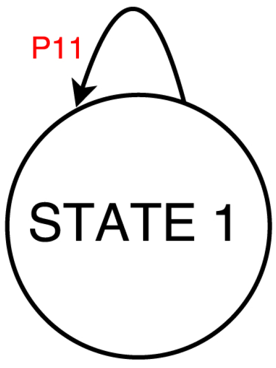Figure 1 and Figure 3 show the state machine and transition probability matrix that we obtained for a washing machine, respectively.

5.3. Context-Based Disaggregation

The experimentation has been composed of several phases. Firstly, each context conditioning has been singularly applied to the algorithm and the obtained results have been compared to those obtained in the work by Kolter and Jaakkola [9]. Secondly, disaggregation results have been evaluated considering both context information items. Each test has been performed by providing the system with the full-knowledge regarding each appliance that could compose the aggregated consumption trace (Table 4), i.e., including even those turned off. As mentioned above, the aggregate consumption trace has been composed synthetically by summing the daily traces of each single appliance. In order to create the test set, we combined each daily trace of a given appliance for a given day with all the daily traces of the other appliances. First, we describe how each single context-based conditioning approach operates.

5.4. Usage Statistic Conditioning

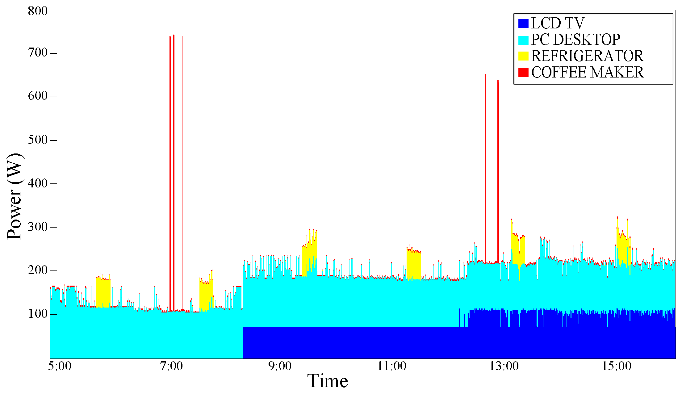
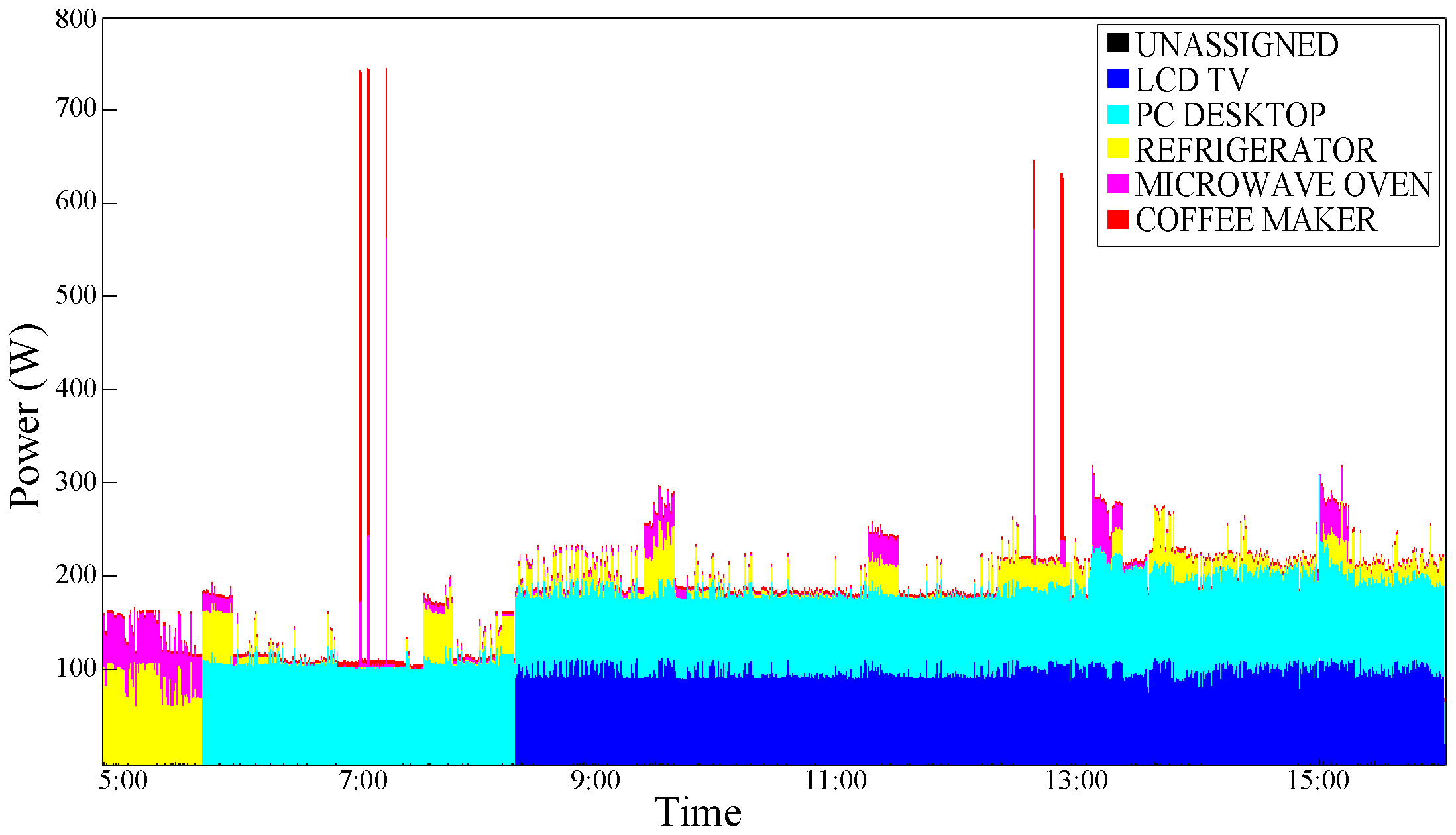
In Figure 6, an aggregate power consumption trace is shown; as it can be noticed in this temporal portion, a PC-Desktop is always ON just like the Refrigerator, an LCD-TV is turned ON a little after 8:00 am and left ON until the end of the examined temporal portion. Moreover, a Coffee Maker is used in the other two daily moments.

Figure 6. Aggregate power consumption trace—test case 1.

Figure 6. Aggregate power consumption trace—test case 1.

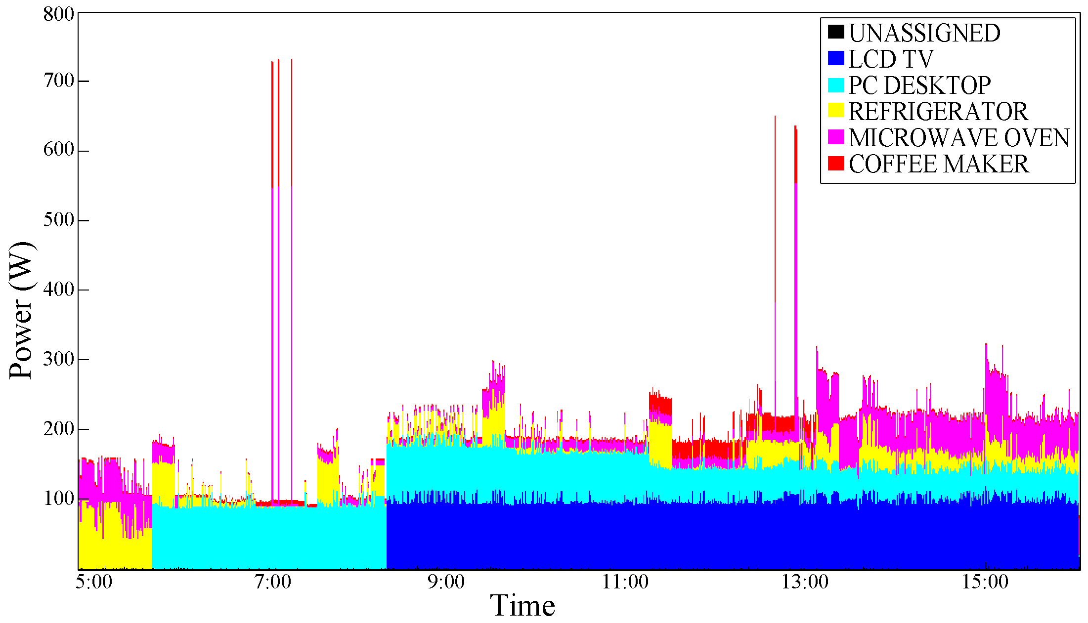
Figure 7 graphically shows the results obtained by applying the disaggregation algorithm by Kolter and Jaakkola [9].

Figure 7. Power consumption trace disaggregated with the basic Kolter and Jaakkola [9]’s Additive Factorial Approximate MAP (AFAMAP) algorithm - test case 1.

Figure 7. Power consumption trace disaggregated with the basic Kolter and Jaakkola [9]’s Additive Factorial Approximate MAP (AFAMAP) algorithm - test case 1.

Figure 8 shows the graphical disaggregation results obtained by applying our NILM algorithm with Usage Statistics Conditioning (USC).

Figure 8. Power consumption trace disaggregated with the Usage Statistics Conditioning (USC)—test case 1.

Figure 8. Power consumption trace disaggregated with the Usage Statistics Conditioning (USC)—test case 1.

An improvement can be observed; this is plausible, especially for devices that are typically switched ON and OFF in a portion of a specific time such as the coffee maker. As expected, a typical ”Always ON" device such as the Refrigerator does not benefit from the effects of this type of conditioning.

Table 6. Precision results obtained with Kolter and Jaakkola [9]’s Additive Factorial Approximate MAP (AFAMAP) algorithm in basic and with Usage Statistics Conditioning version.

	AFAMAP [9]	USC
Refrigerator	27.88%	30.77%
LCD-TV	99.28%	100.00%
PC-Desktop	50.99%	74.07%
Coffee Maker	36.14%	77.21%

Table 6. Precision results obtained with Kolter and Jaakkola [9]’s Additive Factorial Approximate MAP (AFAMAP) algorithm in basic and with Usage Statistics Conditioning version.

	AFAMAP [9]	USC
Refrigerator	27.88%	30.77%
LCD-TV	99.28%	100.00%
PC-Desktop	50.99%	74.07%
Coffee Maker	36.14%	77.21%

Table 6 shows the precision obtained with the timing usage statistics conditioning compared with those obtained by using the AFAMAP algorithm [9].

5.5. User Presence Conditioning

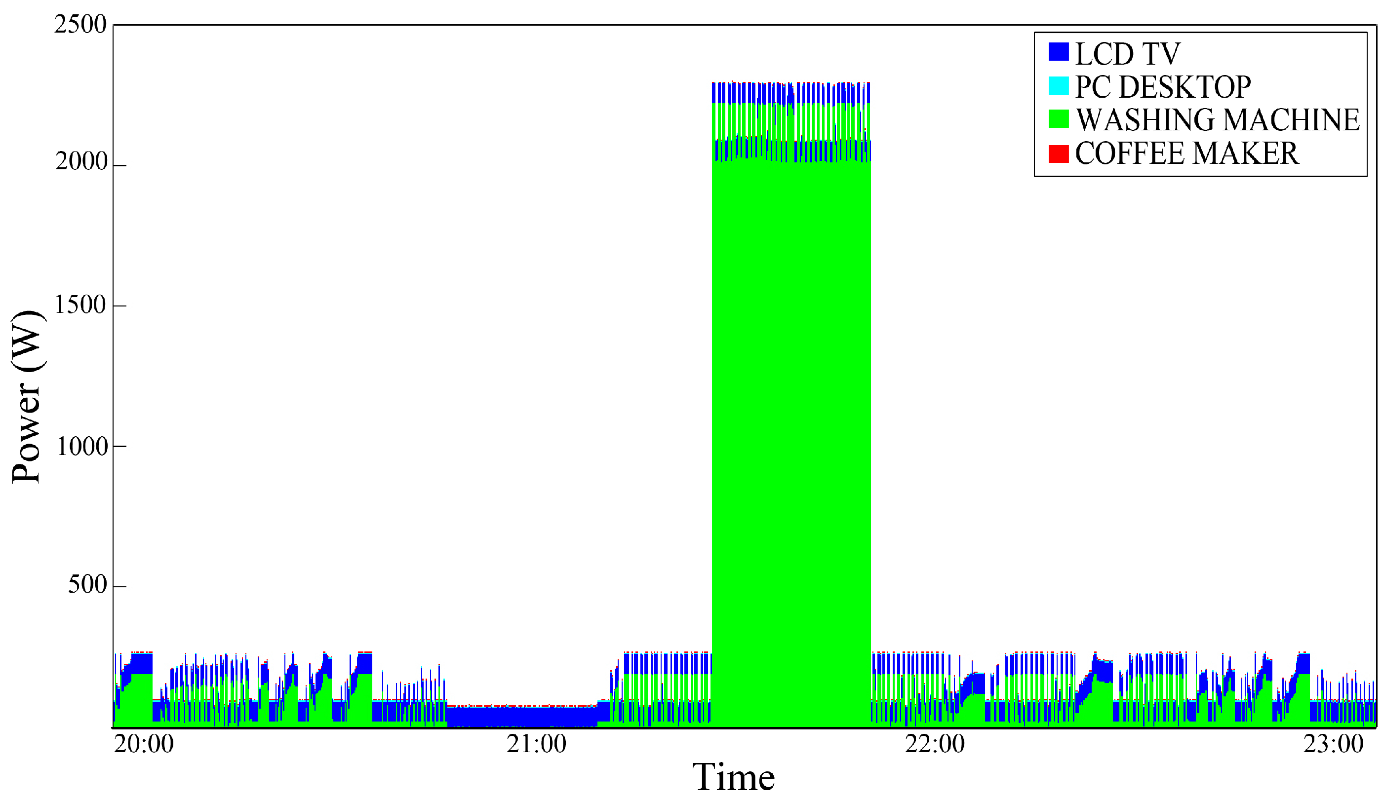
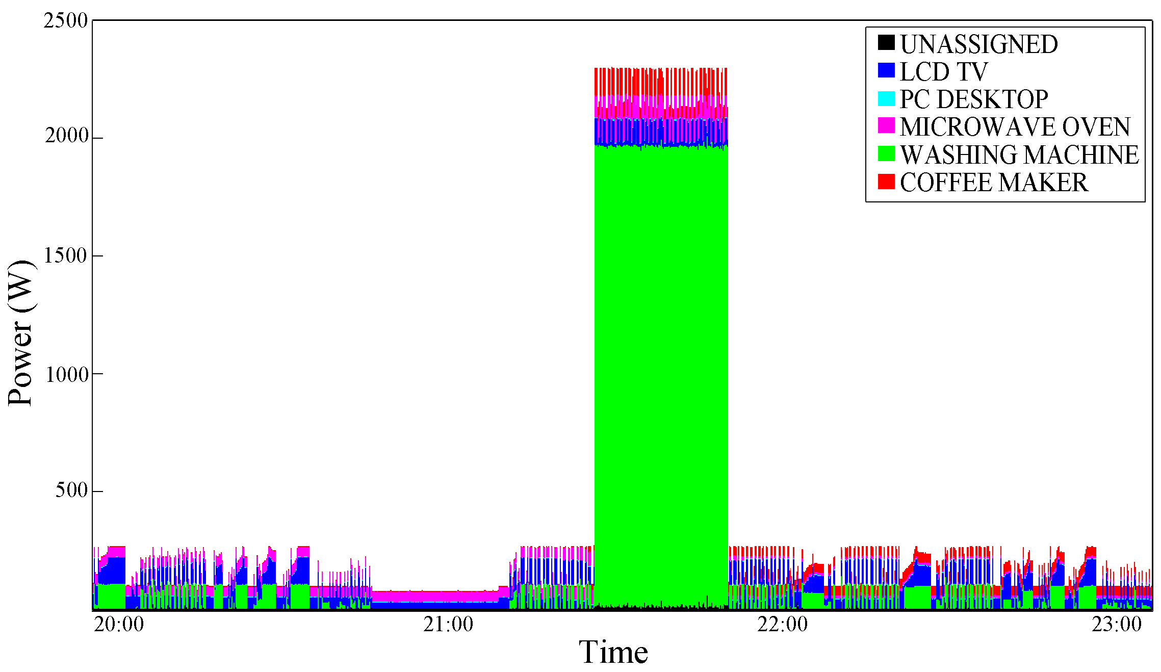
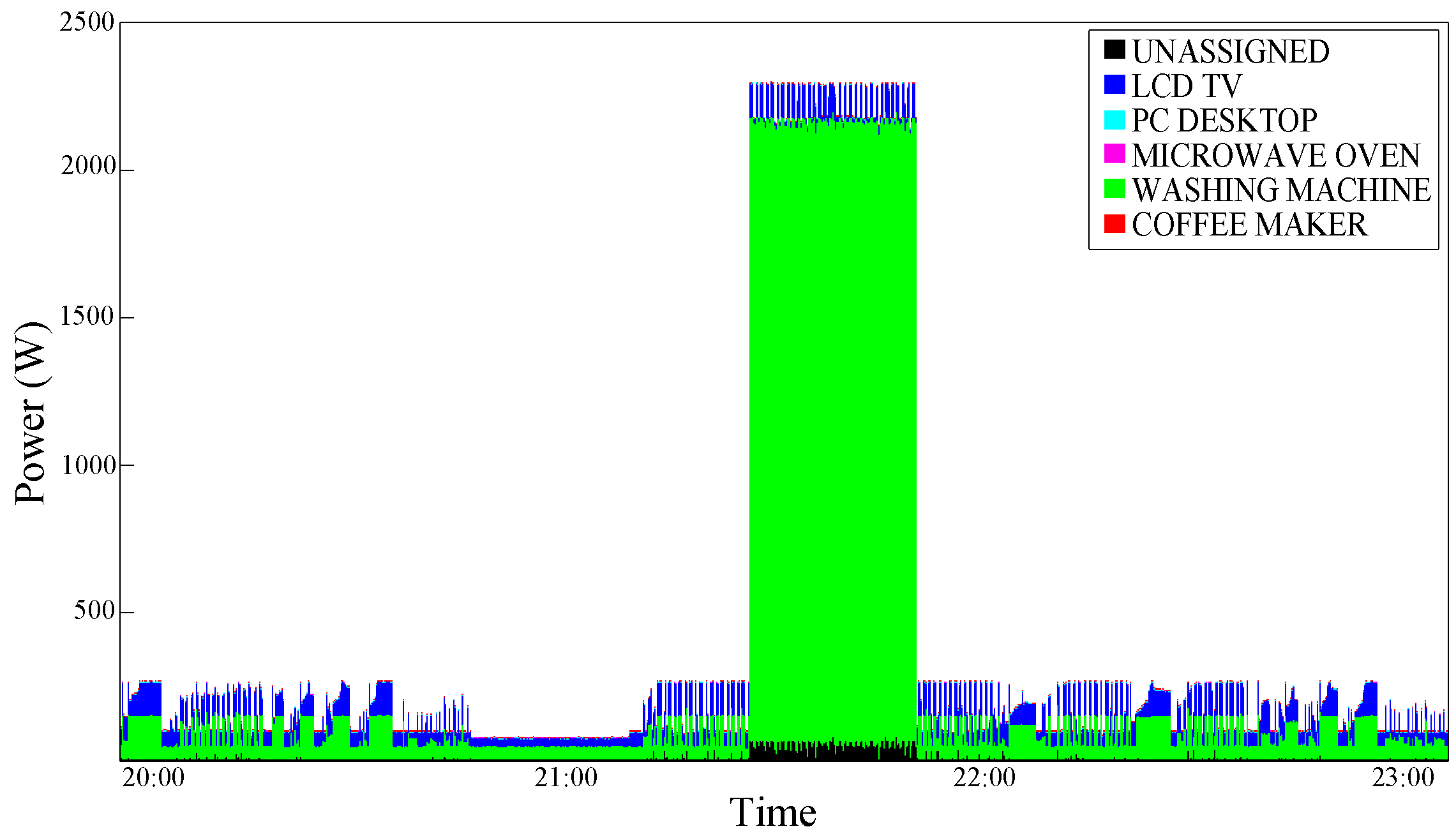
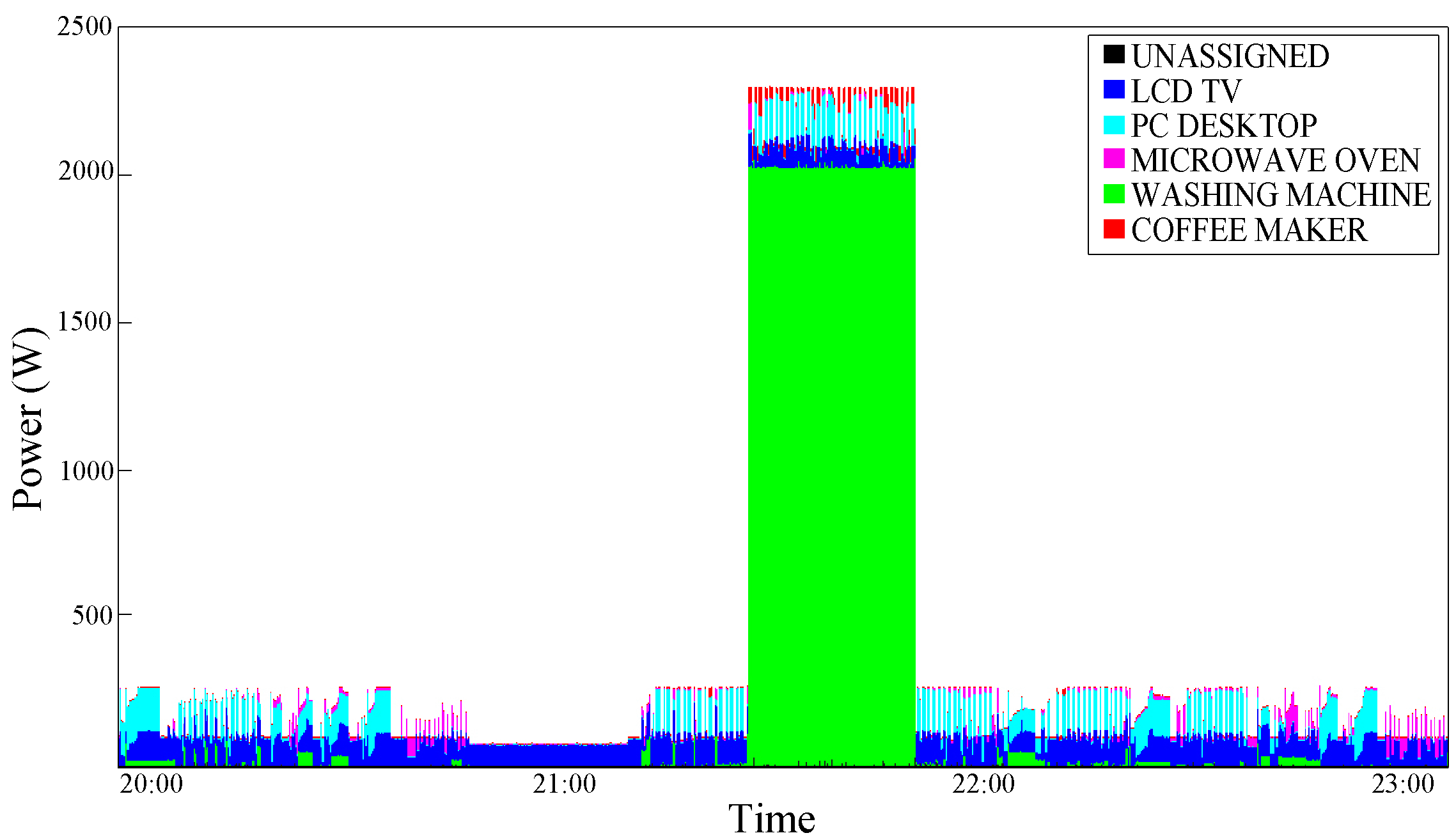
The second conditioning is analyzed below. Figure 9 shows the real aggregate consumption trace of a Washing Machine with the same LCD-TV trace that has been analyzed above; the graphic shows a portion of washing cycle with a high consumption phase (corresponding to the water heating phase) in the middle. In this case, the LCD-TV disaggregation is a little worse (demonstrating that depending on the device traces combination, disaggregation precision can change) and this kind of conditioning, both in the single (Figure 10) and double (Figure 11) interval version, does not introduce relevant improvements with respect to the algorithm by Kolter and Jaakkola [9]. This is due to the fact that in this case the TV usage lasts for a very long period, probably longer than the user presence observation interval. Figure 10 and Figure 11 shows an improvement in the Washing Machine disaggregation, obtained through the Single Interval Conditioning and the Double Interval Conditioning, respectively. The washing phase, which is characterized by low power consumption, is difficultly distinguishable; the basic algorithm, in fact, confuse it for a PC-Desktop execution (Figure 12). Although even with the Single Interval Conditioning few errors are encountered, a portion of washing machine consumption is well-assigned (Figure 10). The graphical results are confirmed by the precision percentage shown in Table 7.

Figure 9. Aggregate power consumption trace—test case 2.

Figure 9. Aggregate power consumption trace—test case 2.

Figure 10. Power consumption disaggregation obtained with the UP Single Interval Conditioning—test case 2.

Figure 10. Power consumption disaggregation obtained with the UP Single Interval Conditioning—test case 2.

Figure 11. Power consumption disaggregation obtained with the UP Double Interval Conditioning.

Figure 11. Power consumption disaggregation obtained with the UP Double Interval Conditioning.

Figure 12. Power consumption disaggregation obtained with Kolter and Jaakkola [9]’s AFAMAP algorithm—test case 2.

Figure 12. Power consumption disaggregation obtained with Kolter and Jaakkola [9]’s AFAMAP algorithm—test case 2.

Table 7. Precision percentages comparison between Kolter and Jaakkola [9]’s AFAMAP algorithm and the User Presence Single and Double Interval Conditioning.

	AFAMAP [9]	UP Single IC	UP Double IC
Refrigerator	70.73%	78.50%	94.78%
LCD-TV	93.86%	90.54%	94.04%

Table 7. Precision percentages comparison between Kolter and Jaakkola [9]’s AFAMAP algorithm and the User Presence Single and Double Interval Conditioning.

	AFAMAP [9]	UP Single IC	UP Double IC
Refrigerator	70.73%	78.50%	94.78%
LCD-TV	93.86%	90.54%	94.04%

5.6. Discussion

Table 8 compares average results of four tests using the basic Kolter and Jaakkola [9]’s algorithm, the User Presence Single Interval Conditioning, the User Presence Double Interval Conditioning, the Usage Statistics Conditioning and a combination of the last two conditioning mechanisms executed together. In almost all cases, a disaggregation precision average improvement is observed with respect to the basic algorithm. Even if the combination of the usage statistics conditioning with the double interval conditioning is better in most cases, percentage-wise, the most effective is the User Presence Double Interval Conditioning. As regards the Recall parameter, the average results are a little worse than the precision ones. This is caused by the nature of this parameter that, by definition, also considers the wrongly assigned or unassigned samples of a given device. However, the recall improvement over the basic algorithm tightly depends on the analyzed test case, as, for example, a greater quantity of not assigned power samples can worsen this value.

Table 8. Average precision/recall percentage results comparison among each tested algorithm for 4 test cases.

	AFAMAP [9]	UP Single IC	UP Double IC	USC	UP Double IC + USC
Test 1	44,72/73,88	61,23/81,11	61,44/74,12	48,68/72,98	61,36/73,84
Test 2	49,63/80,49	43,06/69,39	57,48/70,46	57,40/73,45	58,18/70,68
Test 3	44,37/81,73	54,83/86,97	69,11/71,59	54,18/80,74	68,94/71,43
Test 4	50,76/59,51	41,52/70,74	53,27/55,26	53,43/55,01	52,92/54,38

Table 8. Average precision/recall percentage results comparison among each tested algorithm for 4 test cases.

	AFAMAP [9]	UP Single IC	UP Double IC	USC	UP Double IC + USC
Test 1	44,72/73,88	61,23/81,11	61,44/74,12	48,68/72,98	61,36/73,84
Test 2	49,63/80,49	43,06/69,39	57,48/70,46	57,40/73,45	58,18/70,68
Test 3	44,37/81,73	54,83/86,97	69,11/71,59	54,18/80,74	68,94/71,43
Test 4	50,76/59,51	41,52/70,74	53,27/55,26	53,43/55,01	52,92/54,38

The experimentation campaign, carried out with the complete test set over the basic algorithm for each conditioning, has highlighted the average improvements that have been reported in Table 9.

Table 9. Average Precision and F-Measure improvements over the basic AFAMAP algorithm [9].

	Context-Based Conditionings	Precision	F-Measure
1	User Presence single interval conditioning	$\approx 3\%$	$\approx 2\%$
2	User Presence double interval conditioning	$\approx 12\%$	$\approx 14\%$
3	Usage Statistics conditioning	$\approx 6\%$	$\approx 3\%$
4	The combination of 2) and 3)	$\approx 13\%$	$\approx 14\%$

Table 9. Average Precision and F-Measure improvements over the basic AFAMAP algorithm [9].

	Context-Based Conditionings	Precision	F-Measure
1	User Presence single interval conditioning	$\approx 3\%$	$\approx 2\%$
2	User Presence double interval conditioning	$\approx 12\%$	$\approx 14\%$
3	Usage Statistics conditioning	$\approx 6\%$	$\approx 3\%$
4	The combination of 2) and 3)	$\approx 13\%$	$\approx 14\%$

As can be observed, even though the recall parameter apparently worsened the disaggregation results at test level, the F-Measure evaluation parameter, through the whole test set, reports a significant improvement as well as the precision parameter.

6. Conclusions

In this article, we proposed a new energy disaggregation algorithm that takes into account context-related information that can be gathered from low-cost sensors and statistical analysis of energy consumption data. With respect to most existing works, which are based on the analysis of data collected at a high sampling frequency [14,25,26], our contribution consisted of investigating a disaggregation approach on energy monitoring data collected at low frequency. This choice has the following advantages: it is possible to use low-cost and widely available smart meters and data storage and transfer tasks are less resource demanding. Context features (e.g., user presence and device usage consumption patterns) have been exploited to improve the statistical model of each appliance.

Results of testing activities and their comparison with a state of the art solution are encouraging. In the future, it would be useful to extend the proposed approach to include the use of additional context information (e.g., profile of users, weather information, etc.) in order to improve the disaggregation algorithm as well as to enhance the proposed approach with optimization algorithms and suggestion mechanisms to help consumers in saving energy costs.

Moreover, tests described in this work are based on the use of data available from a publicly accessible dataset, i.e., Tracebase [10]. We believe that the adoption of open data sets in this field may speed up research and innovation processes by favoring repeatable research and easing the comparison of different approaches.