Priority Queues with Fractional Service for Tiered Delay QoS

Abstract

Packet scheduling is key to quality of service (QoS) capabilities of broadband wired and wireless networks. In a heterogeneous traffic environment, a comprehensive QoS packet scheduler must strike a balance between flow fairness and access delay. Many advanced packet scheduling solutions have targeted fair bandwidth allocation while protecting delay-constrained traffic by adding priority queue(s) on top of a fair bandwidth scheduler. Priority queues are known to cause performance uncertainties and, thus, various modifications have been proposed. In this paper, we present a packet queueing engine dubbed Fractional Service Buffer (FSB), which, when coupled with a configurable flow scheduler, can achieve desired QoS objectives, such as fair throughputs and differentiated delay guarantees. Key performance metrics, such as delay limit and probability of delay limit violation, are derived as a function of key FSB parameters for each delay class in the packet queueing engine using diffusion approximations. OPNET simulations verify these analytical results.

1. Introduction

Packet scheduling is central to high-speed routing networks that leverage statistical multiplexing of traffic flows to maximize bandwidth efficiency. In these networks, bandwidth contention arisen from traffic burstiness may result in occasional congestion at a packet router or a network access point. During periods of congestion, a well-designed packet scheduler is needed to allocate bandwidth to competing traffic flows from various classes of users and applications to maintain their required or contracted quality of service (QoS) levels, in terms of queuing delay, packet loss, or throughput. In this environment, QoS contracts can only be fulfilled with a non-zero probability of violation.

A great deal of packet scheduling research has focused on fair allocation of bandwidth [1,2,3,4]. These contributions emphasize the throughput aspect of QoS and deal primarily with flow scheduling. In these cases, the scheduler essentially treats packets solely on the QoS status of their owner flows. One drawback of flow schedulers is that delays of individual packets are not accounted for and, thus, access delays for short-lived traffic flows are not protected. Furthermore, packet retransmissions may occur due to excessive packet delays even when the flow-level fairness is maintained. As Internet and mobile applications become increasingly bandwidth demanding and multimedia driven, maintaining fairness while providing protection for delay sensitive multimedia data plays an important role in modern network design and management.

As packets associated with different traffic flows may have similar delay limits as determined by the flow scheduler, they can be grouped and treated equally as a delay class. One simple approach to differentiate delays between classes is to use priority queues. However, strict priority queues are known to cause highly uncertain delays on all classes except the highest. To provide meaningful packet delay protections, every delay class must receive a certain fraction of service relative to the higher-priority classes to prevent starvation when higher priority classes present heavy loads. This notion of fractional service is the main motive of this work.

We shall present a two-stage packet scheduling architecture that can be tailored to satisfy both flow-level throughput fairness and packet-level delay protections. The first stage is a buffer-less flow scheduler of which the responsibility is to classify packets based on their flow QoS. No specific flow QoS strategies will be assumed except that each classified packet is given a delay limit associated with its assigned delay class. The second stage is a packet queueing engine that uses as many buffers as delay classes to queue classified packets. Its responsibility is to protect the delay guarantee of each delay class such that it is met with a sufficiently high probability. This paper focuses on the second stage: the packet queueing engine. We shall present and analyze the packet queueing engine dubbed Fractional Service Buffer (FSB) that allows a fraction of lower-priority (higher-delay-limit) traffic class to advance their queueing priority at every higher-priority packet arrival. The fraction, in conjunction with the buffer size, determines a delay limit and a delay-violation probability associated with each delay class. Basically, our approach adds a fair queueing component to the conventional static priority queues, such that the lower-priority traffic may improve their priority over time and thus will not be shut out by higher-priority traffic.

The rest of this paper is organized as follows. In Section 2, we cite some related literatures in flow scheduling and priority-queueing schemes. In Section 3, we present the two-stage FSB architecture and its fractional service algorithm. In Section 4, we analyze the FSB under heavy traffic conditions using a combination of queue aggregation technique and diffusion approximations. In Section 5, we demonstrate the accuracy of our analytical results from Section 4 using simulations. In Section 6, we discuss the relationship between the system parameters and desired QoS levels and how tradeoffs between different QoS levels can be achieved. In Section 7, we provide a concrete design example on tuning the FSB system parameters.

2. Related Works

In terms of providing better packet delay for each traffic flow, the scheduler in [5] separates traffic flows with substantially different bandwidth requirements into different groups. Then, a time-stamp based scheduler is used to schedule the service of each group while a round-robin scheduler is used to service flows within a group. However, due to its round-robin structure, there is an inherit dependency between the allocated bandwidth of a flow and the queueing delay of the flow’s packets [6]. Furthermore, only the first packet of each flow can receive a delay protection.

In [6], the authors presented a two-stage architecture that separates the dependencies between bandwidth allocations and packet delays. The first stage is a number of rate regulators that shape the traffic of each flow while the second stage is a number of strict priority queues that queue the regulated packets of each flow. Delay protections are achieved using an admission control policy that monitors the occupancy level at each priority queue. This implementation requires one buffer per flow to regulate each flow’s packets, in additional to the priority queues. These flow buffers require a separate management algorithm to ensure efficient usages of the memory space [7].

Class-based schedulers, on the other hand, have a far simpler approach in managing the memory space. In the Relative Differentiated service (RD) [8] framework, packets are grouped into M + 1 classes of service where Class-i packets receive better performance metrics than Class-i + 1 packets for all 0 ≤ i < M. One simple way of realizing RD is to use strict priority queues where the highest priority class is assigned to the highest priority queue and each queue is serviced in the order of their priority. However, such a method does not provide any means for adjusting the quality of each priority class and no delay protections can be offered to lower priority classes.

In terms of overcoming the inflexibilities of strict priority queues, the authors of [8] presented a delay-ratio idea for determining service orders of each priority class. Specifically, they defined a delay ratio between every pair of service classes and the scheduler strives to maintain these service ratios at their target levels. In this manner, the relative service quality in terms of packet delays between classes is maintained, regardless of the load of higher-priority classes. The authors also applied their delay-ratio idea to existing queueing disciplines, such as Generalized Processor Sharing [9] and Waiting-Time Priority [10], to deliver controllable service qualities. This approach only offers a single dimension in QoS provisioning, namely the delay-ratio between classes. Separate mechanisms are required to ensure the fairness and maximum delay of each traffic class [11].

Other related literature, such as delay-dependent priority jumps [12], deals with this strict priority issue by prioritizing each packet based on its delay limit and tagging the packet with its entry time. The priority of a packet is increased if the maximum queueing delay of the packet in a priority queue is reached. This method requires tagging and updating timestamps of packets to accomplish priority increases.

In [13], the authors presented several priority-jumping policies for systems with two priority classes. Each policy has a unique criterion for increasing the priority of lower priority packets. They concluded that each policy has its pros and cons and no single policy is a clear winner. The system that bases its priority increase criterion on the arrival of higher priority packets is the most “self-adaptive” to different traffic conditions. However, obtaining an exact analytical expression for this system is “extremely difficult”.

3. Fractional Service Buffers

Although commonly referred to as “packet schedulers”, throughput-based schedulers are essentially flow schedulers. Examples of these include Deficit Round Robin (DRR) [14], Weighted Round Robin (WRR), and Weighted Fair Queueing (WFQ) [9] schedulers. However, throughput contracts are meaningful for traffic flows rather than individual packets. Service order of packets is determined solely by flows’ QoS attributes in a flow scheduler. Typically, a flow scheduler uses one queue for each active traffic flow and serves these flow queues with a scheduling discipline to fulfill their throughput contracts. In any of these scheduling solutions, packet delays of a given traffic flow vary with the flow’s packet arrival pattern and the overall system load. As a result, while the throughput of a traffic flow is protected, individual packet delays are not. For short traffic flows, the throughput may not be a meaningful QoS metric since their durations are just a few packets. The quality of these short flows’ services is better represented by their packet delays. Because the majority of traffic flows in the Internet are short [15], packet delays of these flows are a critical contributor to user experience. Furthermore, in a TCP dominated network environment, excessive packet delays may lead to TCP retransmissions thus increasing the duration of congestion.

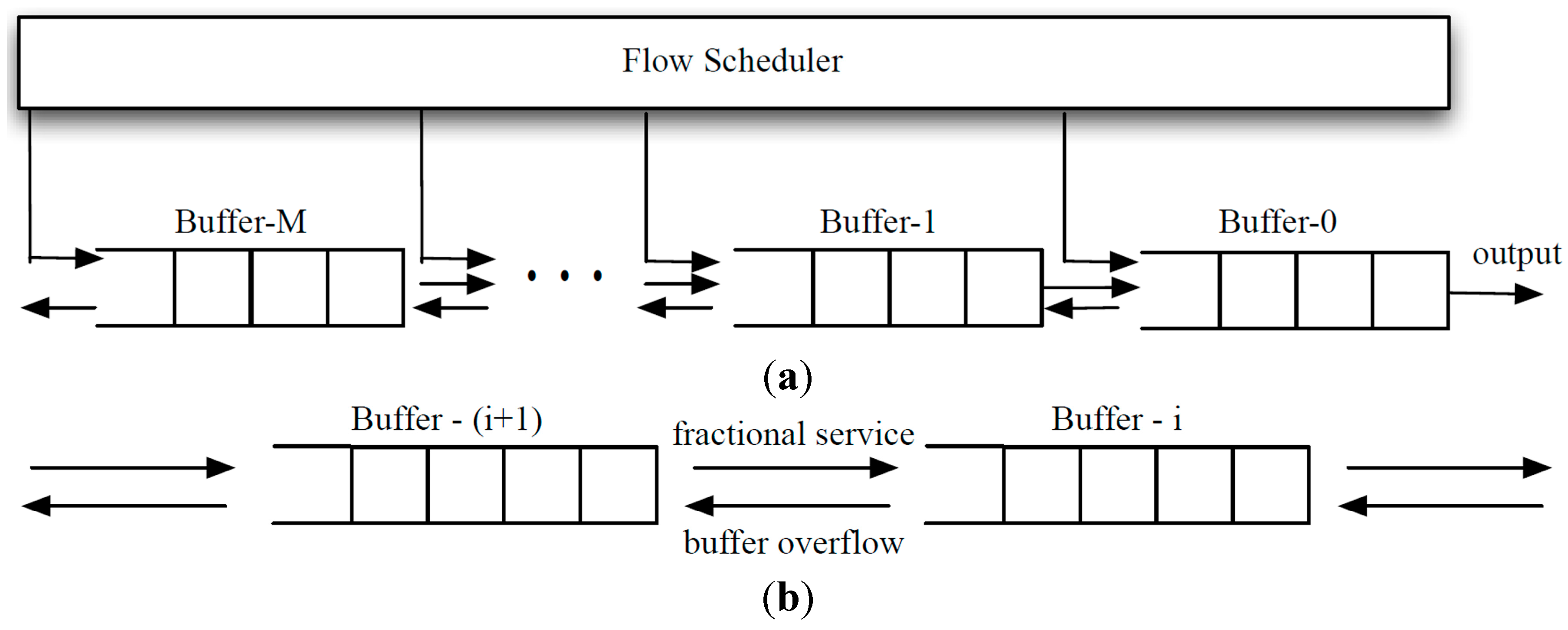
We are presenting a two-stage packet scheduling architecture where the first stage schedules traffic flows and the second stage protects packet delays. In Figure 1, a buffer-less flow scheduler classifies each input packet into a delay class based on its owner flow’s QoS status, while a subsequent packet queueing engine strives to protect the delay limit associated with each class. The flow scheduler maintains flow throughput by specifying a delay limit on each packet. For example, suppose the flow scheduler classifies packets by using a token bucket mechanism with load-adaptive token rates. Instead of physically maintaining a token bucket for each flow in the flow scheduler, the flow scheduler can simply compute the delay limit of each incoming packet based on its flow’s token rate and its available tokens, if any. The packet is mapped accordingly to a delay class based on its delay limit and then sent to the packet queueing engine. Actual packet delay will not reach the specified delay limit unless the system is fully loaded. As such, flows will likely receive more bandwidth than specified by the token bucket algorithm.

Figure 1. Two-stage packet scheduling architecture.

Figure 1. Two-stage packet scheduling architecture.

The simple token bucket algorithm mentioned above for the flow scheduler is merely an example of associating flow throughputs with packet delays. Advanced algorithms, such as WFQ, WF²Q [14] and Least Attained Service [15], which map flow throughputs into packet delays, are also suitable candidates. A flow scheduling policy, in conjunction with the delay protection provided by the packet queueing engine, provides configurable parameters for network operators to tune the desired level of QoS. The key in a configurable QoS scheduler is the packet queueing engine that offers multiple classes of delay protections, where the delay protection of each class can be quantified based on the traffic parameters given by a flow scheduling policy and an admission control policy. In this paper, we are leaving open the flow scheduling policy while assuming that the flow scheduler assigns each packet a delay class according to some selected flow QoS principles. We shall focus on the design and analysis of the packet queueing engine, dubbed the Fractional Service Buffers (FSB), of which the objective is to deliver the packet delay limit of each delay class.

The FSB employs M + 1 FIFO buffers, dubbed Buffer-0, Buffer-1, …, Buffer-M, to accommodate M + 1 classes of classified packets. An arriving Class-i packet is placed in Buffer-i so long as this does not result in a buffer overflow. Basically, Class-0 corresponds to the most delay-sensitive packets and Class-M the least delay-sensitive packets as determined by the flow scheduler. A Class-i packet has a delay limit τ_i to be protected by the FSB, where τ₀ < τ₁ < … < τ_M.

Strict priority queues can be used to differentiate service qualities of multiple classes of traffic. However, strict priority queues, by itself, cannot protect the throughput or the delay of lower-priority classes when higher-priority classes present heavy traffic. Furthermore, the relative service level between traffic classes cannot be quantified or adjusted. The FSB serves its buffers in a strict priority order as well, but it employs a fractional service algorithm (FSA) to “move” packets between buffers in a controlled fashion thus achieving delay guarantees. In the FSB, Class-0 has the highest service priority while Class-M the lowest. Buffer-i earns a unit fractional credit whenever there is a packet arrival from the flow scheduler at ANY of the higher-priority buffers, i.e., Buffer-0, Buffer-1, … Buffer-(i − 1). Once the credit accumulates to one full credit, the packet at the head of Buffer-i is “moved” to Buffer-(i − 1). The credit balance of Buffer-i is then reset to zero. While packet sizes may be used to determine flow fairness in the flow scheduler, packets of different sizes are treated equally by the FSB. We will elaborate on how the FSA moves packets between queues such that a lower-priority class effectively shares a fraction of service with its higher-priority counterpart.

The FSB maintains a credit counter for each buffer except Buffer-0. For every packet arriving at Buffer-i, each lower-priority buffer, Buffer-(i + k), 1 ≤ k ≤ M − i, receives a unit fractional credit of η_i+k = 1/(m(i + k)), regardless of the size of the arriving packet. In other words, Buffer-i receives a credit 1/(mi) whenever a packet arrives at one of the buffers with a priority higher than i (i.e., Buffer-0, Buffer-1, …, Buffer-(i − 1)). The integer m is a configurable parameter used to control the unit fractional credit. When the credit accumulated by Buffer-i reaches unity, its leading packet is moved to Buffer-(i − 1) and is thus “promoted” to Class-(i − 1). A promoted packet is treated equally as any other newly arriving packets to that class. We note that unit fractional credits always accumulate to unity with no leftovers. This would avoid credit remainder issues and their associated analytical and algorithmic complications. Similar to a strict priority queueing system, services are dedicated to a lower-priority buffer when all the higher-priority buffers are empty.

To illustrate the idea behind unit fractional credits, let us consider the case m = 1. In this case, Buffer-1 will receive one full credit for every packet arriving at Buffer-0 from the flow scheduler. Buffer-2 will receive 1/2 of credit for every packet arriving at either Buffer-0 or Buffer-1, from the flow scheduler. Buffer-3 will receive 1/3 of credit for every packet arriving at Buffer-0, Buffer-1, or Buffer-2, from the flow scheduler, and so on. This harmonic descending of the fractional credit with respect to the queue index i is reasonable since the amount of higher-priority traffic included in generating the credit for Buffer-i increases linearly with i.

The configurable integer m controls the rate of promotion of the lower-priority traffic. It can be used as a tuning parameter in defining the QoS levels, in terms of delay limits, for the different traffic classes. A larger m, which implies a slower rate of promotion for lower-priority classes, would favor higher-priority classes, and vice versa. Since packets in Buffer-1 are promoted to Buffer-0 where transmission takes place, Buffer-1 in effect receives 1/(m + 1) of bandwidth. For example, in a 3-Buffer system with m = 1, Buffer-1 effectively receives 50% of bandwidth. It is important to note that Buffer-i carries not only Class-i packets from the flow scheduler, but packets promoted from lower-priority buffers. Packets in Buffer-0 (Buffer-1) may consist of packets from Class-1 (Class-2) that were promoted to Class-0 (Class-1) over time, via the FSA. Similarly, if m = 2, Class-1 and Class-2 packets jointly receive an effective service share of 1/3. If m = 3, Class-1 and Class-2 packets jointly receive an effective service share of 1/4, and so on. Thus, a large m damps the effective service share jointly received by the lower-priority classes thereby increases the delay experienced by these classes. Clearly, when there are many priority classes, a small m should be used to ensure that the lower-priority classes are not shut out from service under heavy traffic conditions.

In order to achieve delay guarantee for each class of packets, we impose an upper limit on the queue length of each buffer. From the perspective of an incoming Class-i packet, the total queue length from Buffer-0 to Buffer-i affects its delay. Unless these higher-priority buffers become empty along the process, Class-i packets have to be promoted, one buffer at a time, from Buffer-i to Buffer-0, in order to receive service. Therefore, instead of constraining the queue lengths of individual buffers, we impose a threshold K_i on the aggregate queue length of Buffer-0 to Buffer-i. That is, the FSB algorithm prevents the total number of packets inside the lowest i buffers, denoted by Q_i, from exceeding K_i. As such, a Class-i packet can enter Buffer-i only if it does not result in Q_i > K_i.

Thus, a Class-i delay violation occurs when a Class-i packet arrives and finds Q_i = K_i. We refer to this event as a packet overflow. An overflowed packet is no longer protected within the delay limit of its priority class originally determined by the flow scheduler. Once a packet overflows from Buffer-i to Buffer-(i + 1), it will be treated as Class-(i + 1) and, thus, receives the delay protection of Class-(i + 1). If Buffer-(i + 1) has also reached its threshold, the packet will be overflowed to Buffer-(i + 2) and so on. Figure 2 illustrates the packet management of the FSB for M + 1 buffers. Figure 2a shows that classified packets from the flow scheduler enter different buffers based on their assigned delay classes. Figure 2b shows packet movements between adjacent buffers based on the FSA, where a rightward arrow signifies packet promotion, while a leftward arrow signifies packet overflow. We note that without buffer capacity thresholds, the FSB becomes strict priority queues when m→∞.

Figure 2. (a) Packets are assigned to different buffers in accordance with their delay classification; (b) Packet movements between buffers as directly by the FSA.

Figure 2. (a) Packets are assigned to different buffers in accordance with their delay classification; (b) Packet movements between buffers as directly by the FSA.

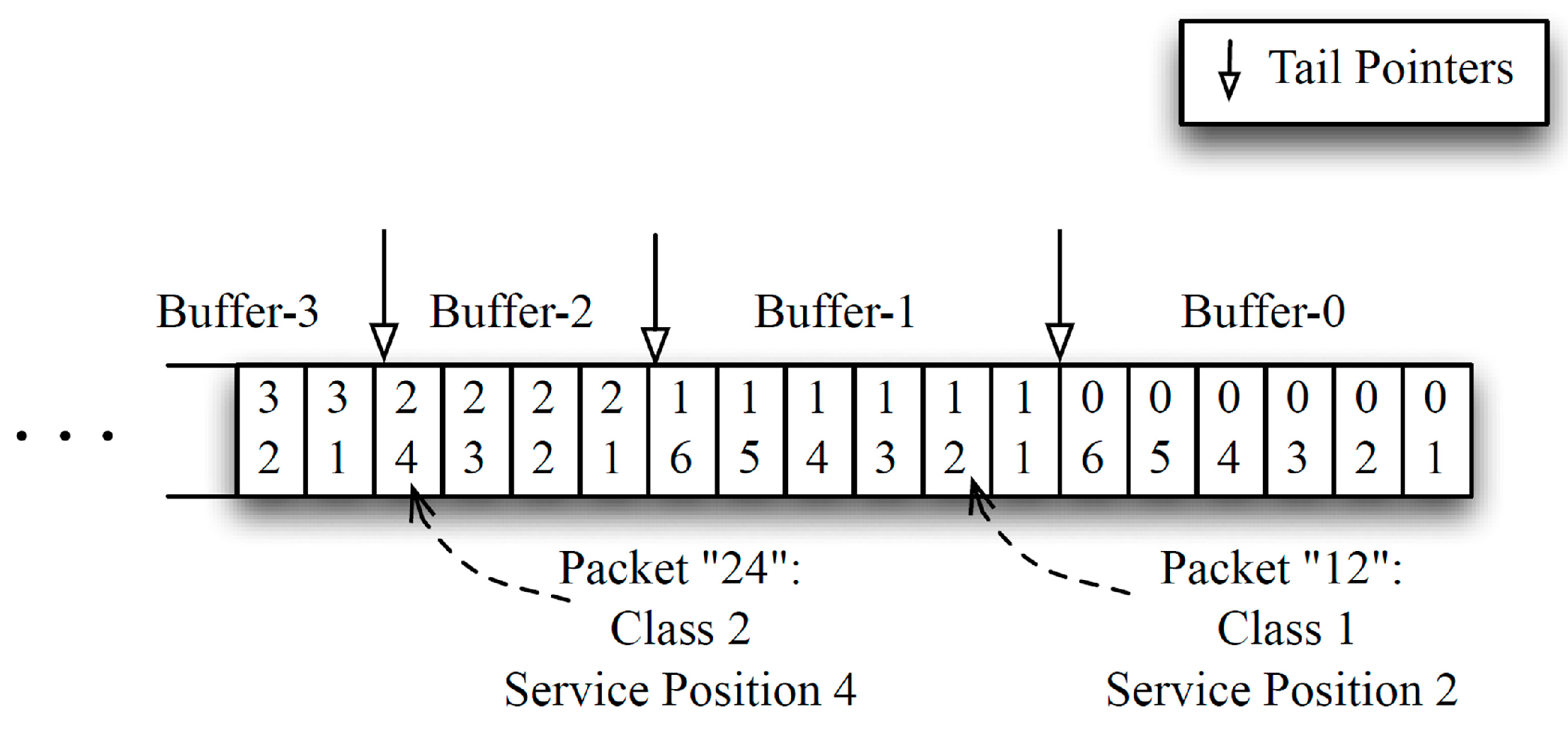
An overflow could occur under two circumstances. To illustrate these scenarios, we label each packet with two integers, ij, where i represents the packet’s current service class and j the position of the packet within the buffer of its class. As shown in Figure 3, we can logically view the buffers concatenated in the order of their priorities. In Figure 4 and Figure 5, we illustrate how the FSB handles these two scenarios with a simple pointer management. The FSB maintains a memory pointer for the tail of each buffer. To illustrate, we assume m = 1 for a 3-buffer system with thresholds K₀ = 6, K₁ = 12, K₂ = 18 for classes 0, 1, and 2 respectively. Figure 4 illustrates the first overflow scenario. In Figure 4a, the arriving Packet X is classified as Class-1 and is supposed to be admitted to Buffer-1. However, the threshold of Class-1 has already been reached (i.e., Q₁ = K₁) at the time. Thus, X has to be overflowed to the tail of Buffer-2 as shown in Figure 4b and counted as a delay violation. In this case, no service credit is awarded to Buffer-2 as a result of X’s arrival because X is not admitted to Buffer-1. Figure 5 illustrates the second overflow scenario. In Figure 5a, Packet Y of Class-0 arrives and is assigned to Buffer-0. In this case, the threshold of Class-0 has not been reached (i.e., Q₀ < K₀) and thus Y can be admitted to Buffer-0. However, the combined number of packets from Class-0 and Class-1, Q₁ will exceed the Class-1 threshold (i.e., Q₁ > K₁) as a result. As shown in Figure 5b one of the Class-1 packets, Packet 18, has to be overflowed to the head of Buffer-2 and counted as a delay violation. This is similar to “push-out on threshold” policies in buffer management [16]. Certainly, the FSB has to limit the frequency of overflow for each class, denoted δ_i for Class-i, to maintain a meaningful delay QoS for that class. In this latter case, the successful insertion of Y grants both Class-1 and Class-2 service credits. Because m = 1, Class-1 and Class-2 receive credits of 1 and 1/2 respectively. As a result, Class-1 has sufficient credit to have its leading packet promoted to Buffer-0 while Class-2 does not. Since promoting a packet from Buffer-1 to Buffer-0 does not change the value of Q₁, the promotion can take place even though Q₁ is at its threshold level Q₁ = K₁. Figure 5c displays the renumbered packets in the buffers after the arrival, the overflow, and the promotion. In particular, Packet Y is now Packet 05, Packet 06 is the promoted Packet 11, and Packet 21 is the overflowed Packet 18 in Figure 5b. We note that each buffer in FSB can be implemented with a link-list and a promotion is achieved by simply moving the tail pointer of the higher-priority buffer by one (packet) to accommodate for the packet promoted from the lower-priority buffer as shown in Figure 5c. In this case, pointer to the tail of Class-0 is moved, while pointer to the tail of Class-1 is not because Class-2 has not earned sufficient credits. With this pointer management scheme, packets do not have to be physically moved once they are placed in the buffer memory.

Figure 3. Logical concatenation of the buffers.

Figure 3. Logical concatenation of the buffers.

Figure 4. First scenario of a packet overflow. K₀ = 6, K₁ = 12, K₂ = 18.

Figure 4. First scenario of a packet overflow. K₀ = 6, K₁ = 12, K₂ = 18.

Figure 5. Second scenario of a packet overflow. K₀ = 6, K₁ = 12, K₂ = 18.

Figure 5. Second scenario of a packet overflow. K₀ = 6, K₁ = 12, K₂ = 18.

4. Performance Analysis

In this section, we perform queueing analysis for the FSB presented in Section 2. Specifically, we use diffusion approximations and a queue aggregation technique to deduce the probability of overflow for each delay class under heavy traffic conditions. Our analytical results demonstrate how the delay limit for each delay class can be enforced by using proper values of FSB parameters: the unit fractional credit and the buffer capacity. To illustrate our analysis, consider the highest-priority buffer of a two buffer case: Buffer-0 with threshold K₀. Queueing analysis of Buffer-0 is performed under the assumption that the traffic input rate is sufficiently high.

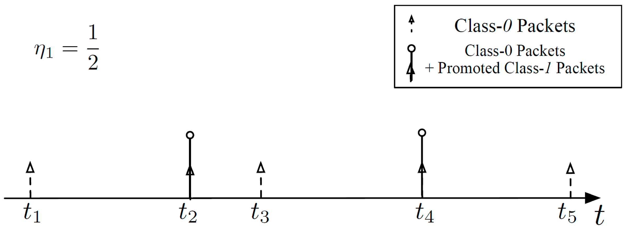
Packets arriving at Buffer-0 from the flow scheduler are assumed to follow a stationary arrival pattern with known mean and variance. Under heavy traffic conditions, we are making an approximate assumption that Buffer-1 always has packets ready to be promoted to Buffer-0 via the FSA. All packet sizes are assumed to follow the same distribution with known mean and variance. Figure 6 shows five sequential Class-0 packet arrivals with η₁ = 1/2. In this example, every other Class-0 packet arrival from the flow scheduler is accompanied by a Class-1 packet promoted to Class-0 from Buffer-1. Thus, the traffic served by Buffer-0 includes Class-0 packets coming straight from the flow scheduler and promoted packets coming from Buffer-1. Essentially, Buffer-0 is a G/G/1/K₀ queueing system where inter-arrival times should account for Class-0 traffic from the flow scheduler and traffic promoted from Buffer-1.

Figure 6. An example of packets arriving at Buffer-0 with η₁ = 1/2.

Figure 6. An example of packets arriving at Buffer-0 with η₁ = 1/2.

We approximate the occupancy of Buffer-0 as a diffusion process of a G/G/1/K₀ queueing system where K₀ is the buffer threshold for Buffer-0. Diffusion process is often used by researchers to model packet schedulers, under heavy load conditions [10], because it leads to closed-form results for the behavior of the scheduler. The key notion is, under heavy traffic conditions, the discontinuities in time from the arrival and departure processes are much smaller than queueing delay. Thus, these processes may be treated as continuous fluid flows, which allow the queue length to be approximated by a diffusion process. For finite buffer cases, the overflow probability can be obtained by imposing boundary conditions on the diffusion process. A comprehensive survey article [17] compared different diffusion approximation techniques and concluded that the diffusion formula by Gelenbe [18] for G/G/1/K queue is the most accurate and robust. It solved the diffusion equation with jump boundaries and instantaneous returns at 0 and K.

A diffusion process is characterized by first and second order statistics of the arrival/departure processes. Let the mean and the variance of packet inter-arrival time be $(\begin{array}{cc}\overline{t,}& {\mathsf{\sigma }}_t^2\end{array})$. For a packet of random size X bits, the mean and the variance of packet service times are denoted $(\overline{X}/C\begin{array}{cc},& {\mathsf{\sigma }}_X^2/C^2\end{array})$, where C represents the service rate in bits/s. Then the probability of the diffusion process touching the boundary K, denoted δ, is given by [18]:

$$\mathsf{\delta }=\mathsf{\beta }(1-\mathsf{\rho })\text{exp}(\mathsf{\gamma }(K-1))$$

(1)

where:

$$\mathsf{\rho }=\overline{X}/(C\overline{t})$$

(2)

$$\mathsf{\gamma }=-2(1-\mathsf{\rho })/(\mathsf{\rho }{\mathsf{\sigma }}_t^2/{\overline{t}}^2+{\mathsf{\sigma }}_X^2/{\overline{X}}^2)$$

(3)

and:

$$\mathsf{\beta }=\mathsf{\rho }{(1-{\mathsf{\rho }}^2\text{exp}(\mathsf{\gamma }(K-1)))}^{-1}$$

(4)

Let the mean and the variance of packet inter-arrival time for Buffer-0 from the flow scheduler be $(\begin{array}{cc}{\overline{t}}_0,& {\mathsf{\sigma }}_{t_0}^2\end{array})$. Also, assume that Buffer-1 has an unlimited supply of packets to be promoted. Since Buffer-0 has to deal with packets from the flow scheduler and packets promoted from Buffer-1, we define the effective packet inter-arrival time, t₀*, as the time interval between two successive packets entering Buffer-0, regardless of the packets’ origins. Then, it is readily shown that the mean and the variance of t₀* are:

$$({\overline{t}}_0*,{\mathsf{\sigma }}_{t_0*}^2)=\left(\begin{array}{cc}\frac{\overline{t_0}}{(1+{\mathsf{\eta }}_1)},& {\left(1-\frac{{\mathsf{\eta }}_1}{1+{\mathsf{\eta }}_1}\right)}^2{\mathsf{\sigma }}_{t_0}^2+\frac{{\mathsf{\eta }}_1}{1+{\mathsf{\eta }}_1}{\overline{t}}_0\end{array}\right)$$

(5)

Under the assumption that the packet arrival process remains stationary, we can substitute Equation (5) into Equations (1)–(4) to obtain δ₀, the probability that Buffer-0 is at its threshold K₀ when a new Class-0 packet arrives. This is the probability of delay limit violation for Class-0 and it depends on the effective load of Buffer-0, ${\mathsf{\rho }}_0^{*}=\overline{X}/(C{{\overline{t}}_0}^{*})$. 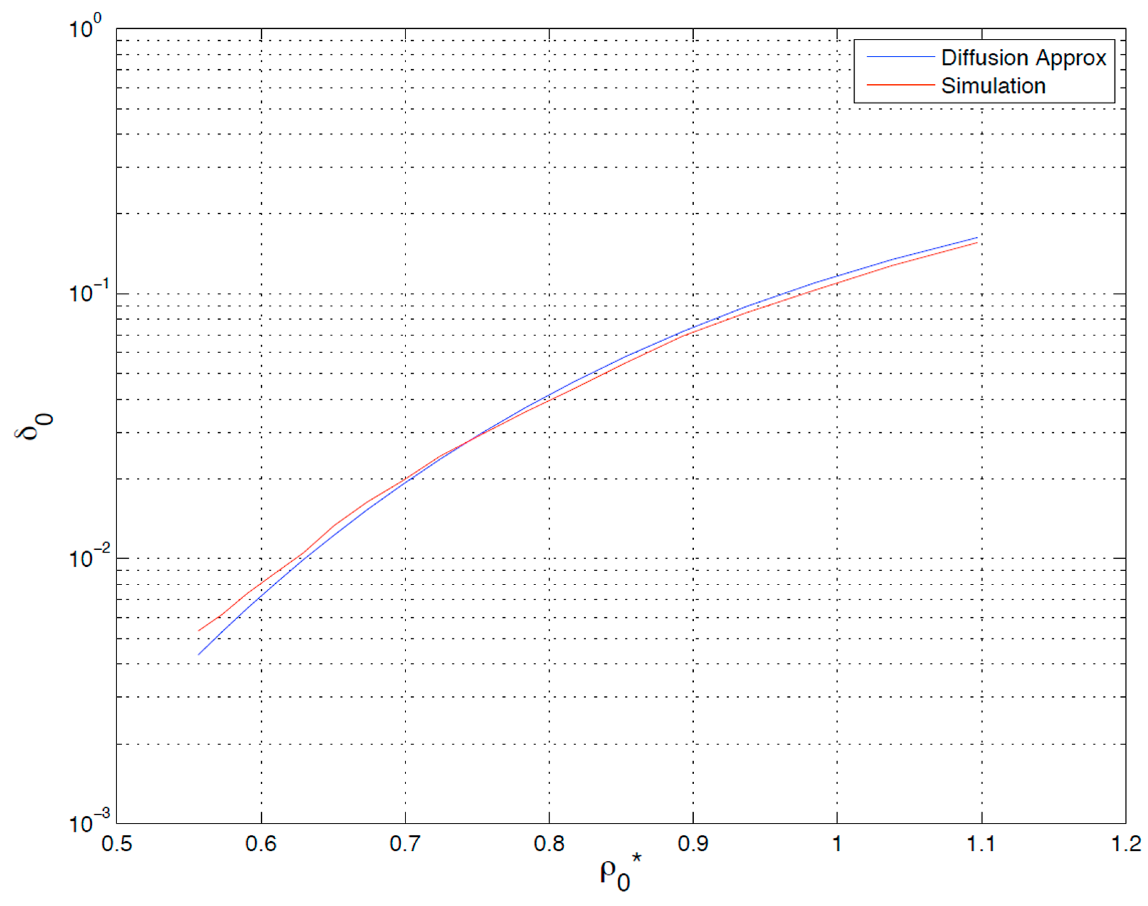For m = 2, a two-buffer system (M = 1) with exponentially distributed inter-arrival time and exponentially distributed service time, Figure 7 shows the simulation result for δ₀ as a function of ${\mathsf{\rho }}_0^{*}$ almost coincides with our result based on diffusion approximations.

Figure 7. Analytical versus simulation results: probability of overflow for Buffer-0 versus its load (2 Buffers, and m = 2).

Figure 7. Analytical versus simulation results: probability of overflow for Buffer-0 versus its load (2 Buffers, and m = 2).

This analytical method can be readily extended to M + 1 buffers, with M > 1. Again, we assume the traffic is heavy and each buffer, except Buffer-0, has traffic ready to be promoted. For each i, we define L_i as the aggregate of packet queues formed in the i + 1 highest-priority buffers (i.e., Buffer-0, Buffer-1, …, Buffer-i), and H_i the aggregate of packet queues formed in the M-i lowest-priority buffers (i.e., Buffer-(i + 1), Buffer-(i + 2), …, Buffer-M). 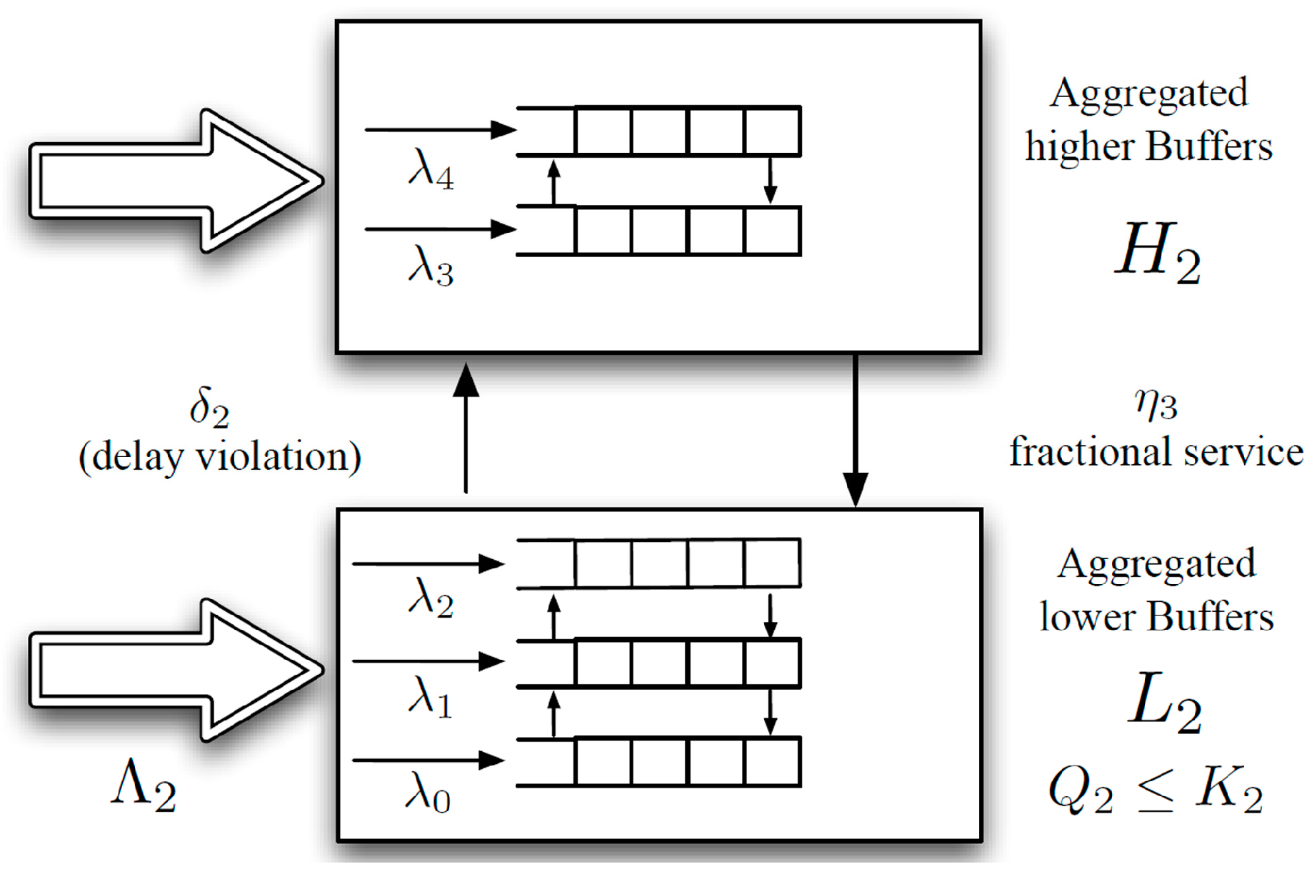Figure 8 shows the aggregate queues L₂ and H₂ for an M = 4 system (5 buffers). The analytical result for the two-buffer case can then be applied to the two aggregate buffers, L_i and H_i.

Figure 8. Buffer aggregation for M = 4.

Figure 8. Buffer aggregation for M = 4.

That is, we may treat L_i as a G/G/1/K_i queueing system whose blocking probability corresponds to the probability of overflow for Class-i. From the conservation law of priority queues [10], the distribution of the number of packets in the system is invariant to the order of service, as long as the scheduling discipline selects packets independent of their service times. Since the FSB is packet-size-neutral, work-conserving, and no packets are dropped inside L_i, we can apply the conservation law to the lower aggregate buffer L_i and use the diffusion result of G/G/1/K_i to find the probability of Q_i = K_i when a new packet arrives at L_i. Interested reader may refer to Reference [10] for a more comprehensive description on the conservation law of priority queues for modeling queueing system.

Let λ_i denote the packet arrival rate at Buffer-i from the flow scheduler. The aggregate packet arrival rate for L_i coming from the flow scheduler is given by:

$${\mathsf{\Lambda }}_i={\displaystyle {\sum }_{k=0}^i{\mathsf{\lambda }}_k}\equiv 1/{\overline{t}}_i$$

(6)

Then, under the assumption that H_i is never empty, the effective inter-arrival time for L_i is given by:

$$({\overline{t}}_i*,{\mathsf{\sigma }}_{t_i}^2*)=\left(\begin{array}{cc}\frac{{\overline{t}}_i}{(1+{\mathsf{\eta }}_{i+1})},& {\left(1-\frac{{\mathsf{\eta }}_{i+1}}{1+{\mathsf{\eta }}_{i+1}}\right)}^2{\mathsf{\sigma }}_{t_i}^2+\frac{{\mathsf{\eta }}_{i+1}}{1+{\mathsf{\eta }}_{i+1}}{\overline{t}}_i\end{array}\right)$$

(7)

where:

$${\eta }_{i+1}=1/(m(i+1))$$

(8)

By substituting Equation (7) into Equations (1)–(4), we can obtain δ_i, the probability of overflow for Class-i packets. Finally, we may obtain the overall packet blocking probability P_B of the system by observing that all M buffers can be aggregated to a single buffer L_M and represented by a G/G/1/K_M queue such that P_B = δ_M.

The FSA allows each delay class, except Class-0, to advance, thus receiving a delay guarantee. Specifically, the worst case delay τ_i, for a Class-i packet that is not overflowed, can be expressed iteratively as a function of the maximum packet size from every class, X_max, and the buffer thresholds K_is:

$${\mathsf{\tau }}_i=\frac{X_{\text{max}}(K_i-K_{i-1})}{({\mathsf{\eta }}_i/(1+{\mathsf{\eta }}_i))C}+{\mathsf{\tau }}_{i-1},1\le i\le M$$

(9)

and:

$${\mathsf{\tau }}_0=\frac{X_{\text{max}}{K}_0}{C}$$

(10)

Finally, define the normalized system load to be:

$${\mathsf{\rho }}_M={\mathsf{\Lambda }}_M\overline{X}/C$$

(11)

The throughput of the whole system can be written as:

$$S={\mathsf{\rho }}_M(1-P_B)$$

(12)

5. Simulation

In Section 3, we used diffusion approximations to reach analytical results describing the probability of overflow associated with each class. OPNET simulations were used to validate these results. We note that extensive studies have been done [10,17] on the diffusion approximation with various arrival time and service time distributions. For simplicity, our simulation assumed relative small buffer sizes and exponential distributions for both packet sizes and inter-arrival times. Note that our analytical results are applicable to any buffer sizes with any stationary inter-arrival time and service time distributions. In particular, we consider a five-buffer system with five traffic classes. For m = 1, we set λ_i = λ, 0 ≤ i ≤ 4, and vary λ to study the loading effect on each buffer. The assumption that every buffer, except Buffer-0, always has traffic to be promoted, does not hold in the simulations but is expected to be sufficient under heavy traffic loads. Figure 9 compares our analytical results with the simulation results: they track each other very closely in terms of the probabilities of overflow. These probabilities of overflow do not exhibit any particular trend across different classes. The approximation appears to be slightly less accurate on higher-priority classes; this may be because the effective load of the aggregate lower buffers L_i increases with i and the fact that our analytical result is based on heavy traffic assumptions. Therefore, for small is, our result yields a conservative approximation to the actual probabilities of overflow; the actual probabilities of overflow are expected to be slightly lower than our approximations.

Figure 9. Probabilities of overflow versus normalized system loads. X is truncated exponential with a maximum size four times the mean, K₀ = 10, K₁ = 20, K₃ = 30, K₃ = 40, K₄ = 50.

Figure 9. Probabilities of overflow versus normalized system loads. X is truncated exponential with a maximum size four times the mean, K₀ = 10, K₁ = 20, K₃ = 30, K₃ = 40, K₄ = 50.

6. Discussion

Our two-stage architecture basically separates throughput protection and delay protection into two different modules. The interactions between the stages are summarized by the traffic statistics of packets entering the queueing engine and the engine’s key parameters m and K_i. The analytical results from Equations (1)–(4), (7), and (9) showed the relationships between the worst-case delay, the delay limit violation probability, and the key parameters m and K_i of the queueing engine. By tuning these parameters, the protections offered to each delay class can be altered.

Recall that K_i is the limit on the aggregate queue length of L_i. Supposing that we set these thresholds to be multiples of K₀, i.e., K₁ = 2K₀, K₂ = 3K₀… That is, for each additional service class, we increase the buffer capacity by a constant amount K₀. In this setup, one may expect the worst-case delays of these classes to scale linearly as the priority decreases. However, this is not the case. 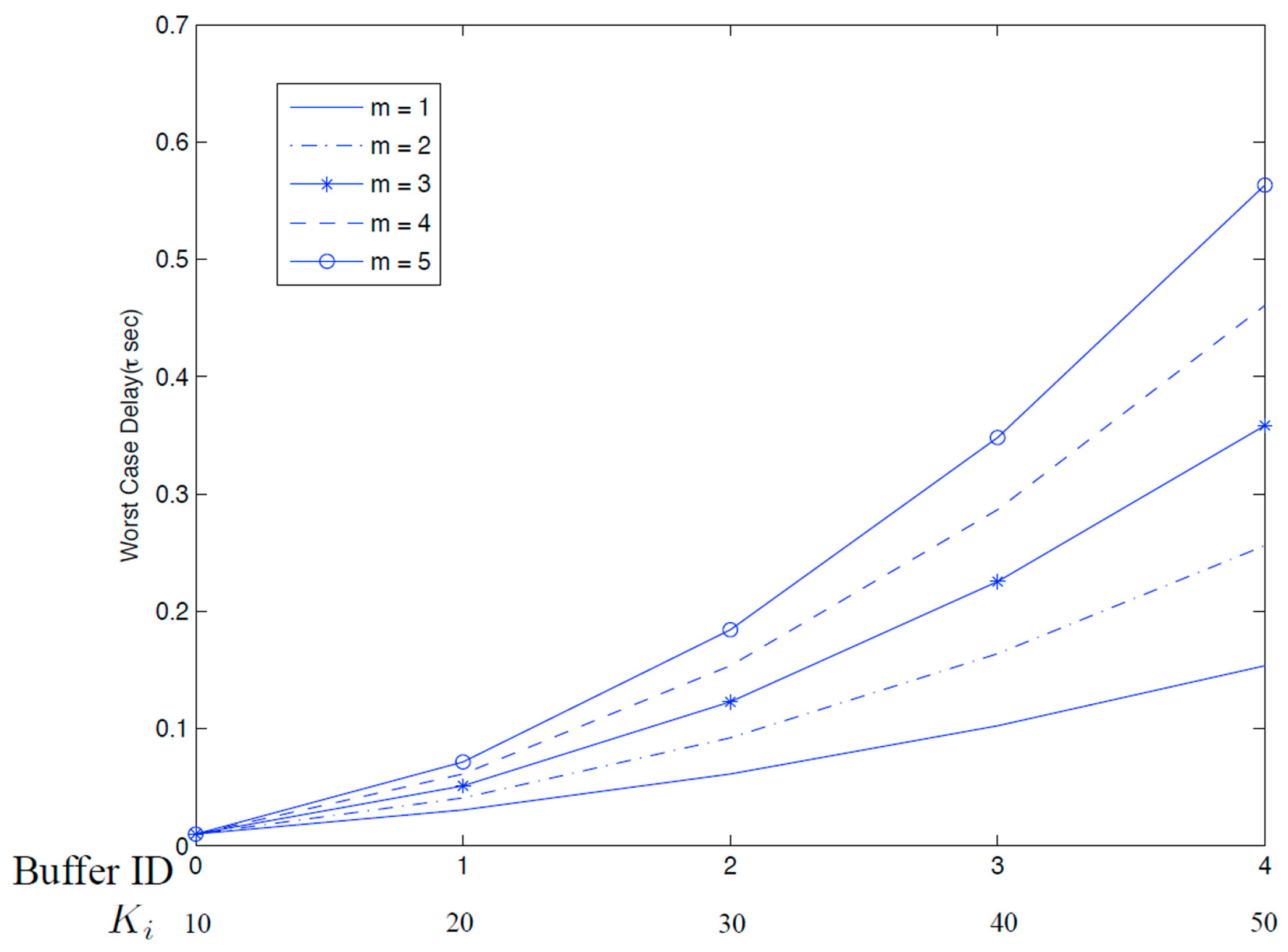Figure 10 plots worst-case delay against priority level, which shows that the increase in delay is faster than a linear rate. This is because the rate of promotion worsens as i increases and for lower-priority buffers (larger i), effects of slower promotion rates compound. This phenomenon is best observed in Equation (9): the difference of the worst-case delays between two adjacent priority classes, τ_i − τ_i−1, has a denominator that decreases faster than a linear rate as i increases. For example, when m = 1, the denominators of τ_i − τ_i−1 are η₁/(1 + η₁) = 0.5, η₂/(1 + η₂) = 1/3, and η₃/(1 + η₃) = 1/4, for i = 1, 2, 3, respectively, while the numerators remain constant with respect to i.

Figure 10. Worst-case delays for buffers when M = 4 and m = 1, 2, …, 5.

Figure 10. Worst-case delays for buffers when M = 4 and m = 1, 2, …, 5.

Changing parameter m affects the rate of promotion and thus the worst-case delay. It can be used to tune the relative service quality level, in terms of packet delays, received by the delay classes, a concept similar to delay-ratios used in [8]. A large m favors higher-priority classes because with a slower promotion rate, the worst-case delays for lower-priority classes would worsen. Figure 10 plots worst-case delays of all the buffers for several values of m. Note that a larger m gives a steeper decrease in the rate of promotion and results in an increasing gap between the curves as priority level increases (i.e., delay limit worsens). A small m should be used when there are many traffic classes to prevent starvation of lower-priority classes.

In this paper, we have imposed a unit fraction η_i = 1/(mi) upon the rate at which Buffer-i can promote its packets. Although this has simplified the analysis and implementation of the FSB considerably, it has also greatly limited its configurability, since a single parameter m controls all the unit fractions η_i. Without such a unit fraction restriction, the values of η_i can be set and tuned individually in order to yield more flexible performance tradeoffs between delay classes. Under this general approach, to lower the worst-case for the ith class, one can choose to either increase η_i or decrease K_i. From the iterative relationship of the worst-case delay, Equation (9), lowering the threshold K_i will naturally lower the delays of all classes i and above. By lowering K_i, the buffer capacity for accommodating packets from the ith class will also be lowered thus leading to a higher delay violation probability for the ith class. Increasing η_i will also lower the worst-case delay of all classes i and above. However, by increasing η_i, we are increasing the service share dedicated to the lower-priority buffers. Thus, even though worst-case delays for higher-priority buffers will not be affected by a larger η_i, their probabilities of delay limit violation will be higher. Basically, favoring some classes inevitably affects the other classes. The tradeoff is determined by the setting of K_i and η_i.

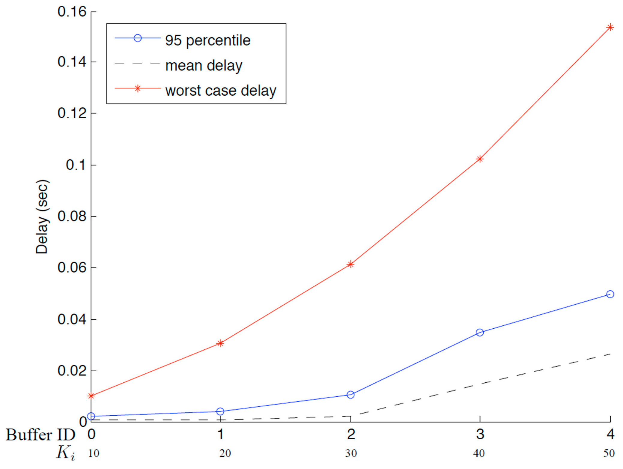
The worst-case delay for the ith class occurs only if all buffers of equal or higher priority are fully occupied, and all packets in these buffers are of the maximum size. Naturally, this is a pessimistic upper bound for the delay. Figure 11 plots worst-case delays and the 95-percentiles of packet delays for the 5-buffer case when m = 1. Packet sizes are assumed to follow a truncated exponential distribution with a maximum packet size four times the mean packet size. As can be seen in the graph, worst-case delays, marked by asterisks, are well above their 95-percentiles, marked by circles. Furthermore, the differences between mean packet delays, plotted in dotted line, and worse-case delays are larger for lower priority traffic. This might be caused by the pessimistic assumption that all lower buffers are fully and continuously occupied to reach the worst case. Overall, Figure 11 demonstrates that the majority of packets are protected within their delay-limits promised by the queueing engine.

Figure 11. Delays for a system with M = 4 and m = 1.

Figure 11. Delays for a system with M = 4 and m = 1.

7. Designing Fractional Service Buffer

In the previous section, we showed that, given the values of K_i (i.e., thresholds for the queue length of each L_i) and m, the delay limit and the probability for delay limit violation for each class could be determined. When designing a packet scheduler, however, a common objective is to set the buffer size for each delay class such that a pre-determined delay limit for that class can be achieved. In the following, we illustrate how to utilize our analytical results to achieve this design objective.

We consider a case with M = 4, where each Class-i has a delay limit of (i + 1)D. That is, the delay limit increases with i such that Class-0 has a delay limit of D, Class-1 a delay limit of 2D, Class-2 a delay limit of 3D, and so on. For simplicity, we assume that the packet sizes are fixed and are equal for all classes and let X_max denote the fixed packet size. By letting each τ_i − τ_i−1 = D in Equations (9) and (10), each K_i can be expressed as:

$$K_0=\frac{DC}{X_{\text{max}}}$$

(13)

$$K_i=\frac{{\mathsf{\eta }}_i/(1+{\mathsf{\eta }}_i)DC}{X_{\text{max}}}+K_{i-1},1\le i\le M$$

(14)

The above equations associate each K_i with the delay limits. However, K_is and delay limits are meaningless without being accompanied by the probabilities of delay-limit violation (i.e., δ_i), which can be determined given the packet-arrival statistics. For simplicity, let the packet inter-arrival time for each Buffer-i be exponentially distributed with a mean of 1/λ (i.e., λ_i = λ for all 0 ≤ i ≤ M). We use a numeric example to illustrate the relationships between D, K_i, and δ_i, where the numeric values used in this example are summarized in Table 1. Note that $D=50\frac{X_{\text{max}}}{C}=7.5\times {10}^{-4}$, which is equal to the time required for serving 50 packets of size X_max = 1500. This results in K₀ = 50. Additionally, note that λ is chosen such that the system has a normalized load of 1 (i.e., ${\mathsf{\rho }}_M=\frac{(M+1)\mathsf{\lambda }{X}_{\text{max}}}{C}=1$). This means that ${\mathsf{\rho }}_0=\frac{\mathsf{\lambda }{X}_{\text{max}}}{C}=0.2$, ${\mathsf{\rho }}_1=\frac{2\mathsf{\lambda }{X}_{\text{max}}}{C}=0.4$, and so on. As such, Buffer-0 can store up to 50 Class-0 packets but only has ${\mathsf{\rho }}_0=0.2$ of traffic load. Clearly, Class-0 traffic has ample storage space for storing packets and will have a very small probability of delay limit violation, δ₀, regardless of the unit fraction, η₁ = 1/m, chosen for packet promotion from Buffer-1 to Buffer-0. This excessive storage space is shared with lower-priority classes, thus allowing these classes to enjoy low probabilities of delay limit violation as well. Table 1 illustrates the K_i required for achieving the delay limits when m = 1 and when m = 2. For m = 1, K_i − K_i−1 decreases as i increases. In other words, the dedicated buffer space for Class-i packets under congestion (i.e., K_i − K_i−1) is small when Class-i has low priority. This is because as i increases, η_i decreases harmonically while the delay limit increases linearly. The linear increase on the delay limit requires that each Class-i packet be promoted in D seconds, for any Class-i with 1 ≤ i ≤ M. However, the harmonic descent on η_i implies that a Class-i packet is promoted slower than that of a Class-(i−1) packet. That is, as the promotion rate of packets becomes slower when i increases, the limit on the time for a packet promotion remains unchanged. As a result, the dedicated buffer space for Class-i decreases as i increases. This phenomenon is even more apparent for m = 2, which results in a lower η_i for each Class-i when compared with the m = 1 case. Table 1 also summarizes the probabilities of delay limit violation, where the higher-priority classes have very small probabilities of delay limit violation as expected. Even for Class-4 traffic, which has the lowest priority, its delay limit can be protected with a fairly high probability, when m = 1 and m = 2.

Table 1. Parameters for the Fractional Service Buffer (FSB) design example, and comparison on the Size of aggregated lower buffers (K_i) vs. probabilities of delay limit violation (δ_i).

D (s)	C (bps)		Xmax (bits)		λ
7.5 × 10−4	1.00 × 108		1500		1.33 × 105
m = 1
Class		Ki		δi
0		50		1.26 × 10−22
1		75		7.17 × 10−26
2		91		4.72 × 10−15
3		104		9.50 × 10−3
4		114		8.70 × 10−3
m = 2
Class		Ki		δi
0		50		2.97 × 10−60
1		66		7.37 × 10−48
2		76		1.19 × 10−26
3		83		1.81 × 10−9
4		89		1.11 × 10−3

Table 1. Parameters for the Fractional Service Buffer (FSB) design example, and comparison on the Size of aggregated lower buffers (K_i) vs. probabilities of delay limit violation (δ_i).

D (s)	C (bps)		Xmax (bits)		λ
7.5 × 10−4	1.00 × 108		1500		1.33 × 105
m = 1
Class		Ki		δi
0		50		1.26 × 10−22
1		75		7.17 × 10−26
2		91		4.72 × 10−15
3		104		9.50 × 10−3
4		114		8.70 × 10−3
m = 2
Class		Ki		δi
0		50		2.97 × 10−60
1		66		7.37 × 10−48
2		76		1.19 × 10−26
3		83		1.81 × 10−9
4		89		1.11 × 10−3

8. Conclusions

We have developed a packet queueing engine that queues packets of different delay classes using a fixed number of buffers and a service discipline that strives to deliver a packet delay guarantee to each class. The service discipline serves the buffers in a strict priority order while using a specially designed algorithm to advance packets in lower-priority buffers to higher priority buffers over time. We showed how the tiered delay guarantees can be achieved and how the probabilities of delay limit violation can be analyzed. In particular, we employed diffusion approximations and a queue aggregation technique to derive closed-form relationships between the delay limit and the probability of delay limit violation for each class and the key parameters of the queueing engine. These analytical results can be used to tune the parameters in order to achieve a desired performance objective or a desired tiered delay service objective. The simulation results demonstrated the accuracy of our analytical results. When coupled with a proper flow scheduler such as a token bucket algorithm, the presented packet queueing engine—the FSB—may be configured to yield a comprehensive QoS packet scheduling solution.