LEO Satellite and UAV-Assisted Maritime Internet of Things: Modeling and Performance Analysis for Data Acquisition

Abstract

The integration of low Earth orbit (LEO) satellites and unmanned aerial vehicles (UAVs) into the maritime Internet of Things (MIoT) offers an effective solution to overcoming the limitations of connectivity and transmission reliability in conventional MIoT, thereby supporting marine data acquisition. However, the highly dynamic ocean environment necessitates a theoretical framework for system-level performance evaluation before practical deployment. In this article, we consider a LEO satellite and UAV-assisted MIoT (LSU-MIoT) network and develop an analytical framework to evaluate its transmission performance. Specifically, marine devices and relaying buoys are modeled as a Matérn cluster process on the sea surface, UAVs as a homogeneous Poisson point process, and LEO satellites as a spherical Poisson point process. Signal transmissions over marine, aerial, and space links are characterized by Nakagami-m, Rician, and shadowed Rician fading, respectively, with the two-ray path loss model applied to sea and air links for accurately capturing propagation characteristics. By leveraging stochastic geometry, we derive analytical expressions for transmission success probability and end-to-end delay of regular and emergency data under the time division multiple access and non-orthogonal multiple access schemes. Simulation results validate the accuracy of derived expressions and reveal the impact of key parameters on the performance of LSU-MIoT networks.

1. Introduction

The maritime Internet of Things (MIoT), integrating advanced Internet of Things technologies, is expected to serve as a crucial infrastructure for a wide range of maritime applications, including environmental monitoring, ecological protection, natural disaster prevention, oceanographic research, mineral resource exploration, and maritime security and surveillance [1,2]. These activities generate enormous volumes of heterogeneous and critical marine data that must be efficiently and reliably collected and transmitted. By enabling seamless communication among diverse marine devices (MDs) such as vessels, buoys, sensors, and unmanned surface vessels, the MIoT supports large-scale and continuous acquisition and delivery of marine data to the offshore information center [3,4]. However, due to the vast and sparsely connected oceanic environment, and the absence of wired infrastructure and stable power supply, the unevenly distributed MDs present serious challenges to maintaining reliable connectivity with the shore, critically constraining the delivery of marine data to the offshore information center. In practical marine data acquisition, diverse marine data pose distinct transmission requirements. For instance, time-sensitive data related to maritime search and rescue operations require low-latency and high-reliability transmission, while measurements of water quality or ocean currents, such as temperature and humidity, can tolerate higher latency. Additionally, the highly dynamic, harsh, and unpredictable ocean environment poses severe constraints on the efficiency and reliability of data transmission from MDs to the offshore information center [5]. To this end, unmanned aerial vehicles (UAVs) and low Earth orbit (LEO) satellites, with their high mobility, adaptive deployment flexibility, and wide-area coverage, have emerged as promising entities to extend the connectivity of the MIoT, thereby overcoming the inherent limitations of conventional marine communication architectures. Therefore, the integration of LEO satellites and UAVs into the MIoT, establishing a LEO satellite and UAV-assisted MIoT (LSU-MIoT) network, represents a promising approach to significantly enhance the capability for supporting marine data acquisition.

To enable effective marine data acquisition, a system-level performance evaluation of the LSU-MIoT network is indispensable before its practical deployment. Nevertheless, the inherently dynamic and harsh maritime environment, characterized by intense rainfall, sea surface fluctuations, and complex propagation conditions, renders the accurate characterization of transmission performance particularly challenging [2,6]. Therefore, it is necessary to establish a theoretical framework to model and evaluate the performance of the LSU-MIoT network.

Stochastic geometry has served as a fundamental mathematical framework for the analytical characterization of spatially distributed wireless networks, providing deep theoretical insights into large-scale network performance [7]. Leveraging this framework, recent studies have applied it to evaluate downlink, uplink, joint uplink–downlink, and end-to-end transmission behaviors in maritime networks. For instance, Xu et al. investigated the downlink coverage probability of marine stations on far-reaching sea surface by employing a homogeneous Poisson point process (HPPP) to model various relaying nodes [8]. Then, Xiong et al. analyzed the coverage probability and transmission rate of near-shore and offshore users in an integrated terrestrial–satellite maritime network, where a shore base station and a LEO satellite jointly provide wide-area connectivity to maritime users [9]. Following this, Gao et al. focused on the uplink signal transmission performance of a relay-assisted satellite maritime network, deriving the successful transmission probabilities at both the ship relays and satellites using a non-orthogonal multiple access (NOMA) scheme [10]. Extending to both uplink and downlink communications, Li et al. in [11] used independent PPPs to model satellites and maritime users for assessing downlink and uplink coverage performance in satellite-maritime networks. Furthermore, to capture the end-to-end transmission behavior, our previous work [12] modeled LEO satellites as a homogeneous binomial point process to evaluate the LEO satellites-assisted shore-to-ship transmission performance.

For marine and underwater IoT scenarios, several studies have focused on the topic of data acquisition, physical-layer security, and performance gain analysis by incorporating advanced network entities such as UAVs and LEO satellites, leveraging the tool of stochastic geometry. For instance, Xu et al. [13] derived the best coverage probability and maximized it by optimizing the surface station densities in a K-tier underwater IoT network. Building on this, a three-hop underwater wireless acoustic communication network architecture was developed by deploying relay stations along the sound fixing and ranging layer, and the analytical expression for the three-hop coverage probability was derived to enable long-range underwater communication over thousands of kilometers with enhanced energy efficiency [14]. Addressing the problem of physical-layer security, Li et al. [15] derived closed-form expressions for beam coverage probability and secrecy outage probability in a maritime relay-assisted hybrid satellite–underwater optical communication system. Furthermore, Aman et al. analyzed the effects of random jamming in underwater MIoT networks and derived tractable expressions for overall coverage probability, average rate, and energy efficiency. To evaluate the impact of integrating advanced entities, Hu et al. [3] investigated the uplink coverage probability in a buoy-assisted MIoT scenario by modeling marine devices and buoys as a Matérn cluster process. Then, Senadhira et al. in [16] analyzed the uplink success probability from maritime users to UAVs and subsequently to LEO satellites within a two-phase communication scheme. In terms of data acquisition, Wang et al. [17] proposed a UAV-assisted underwater data collection scheme and developed a theoretical model to analyze path connectivity via intermediate sink nodes under both grid and random deployment strategies.

As aforementioned, despite significant progress in evaluating network performance in maritime and underwater scenarios, research on marine data acquisition in MIoT scenarios remains limited, particularly in distinguishing between the demands of regular and emergency data. Meanwhile, stochastic geometry–based analyses that characterize the latency of marine data acquisition are still scarce. In addition, most existing studies on maritime and underwater networks fail to adequately account for practical signal propagation environments, such as the two-ray path-loss model. Motivated by these limitations, it is crucial to develop a theoretical framework to evaluate the network performance of the LSU-MIoT network. However, accurately characterizing its performance poses several challenges. First, the incorporation of the two-ray path-loss model, which involves complex analytical expressions, exacerbates the analytical difficulty. Secondly, accounting for the influence of interfering MDs on the complex path loss and fading expressions, the task of deriving analytical expressions for the network performance becomes more challenging. Finally, the aggregation of multiple random factors across different links, including distances, fading effects, and randomly assigned time slots, further complicates the modeling. These challenges collectively motivate us to bridge this gap by establishing an analytical framework for characterizing the performance of the LSU-MIoT network.

In this article, we consider an LSU-MIoT network and develop a theoretical framework based on stochastic geometry to analyze its network performance for supporting marine data acquisition. This framework aims to evaluate signal transmission performance across the marine, aerial, and space links, subject to Nakagami-m, Rician, and shadowed Rician fading, respectively. The two-ray path loss model is incorporated into the marine and air links to accurately capture large-scale propagation characteristics. Notably, to the best of our knowledge, this study represents the first attempt within the context of stochastic geometry to analyze the MIoT network performance while considering the transmission of two types of collected marine data, i.e., regular and emergency data. The main contributions of this article are summarized as follows.

• Leveraging stochastic geometry, we derive analytical expressions for the transmission success probability of regular and emergency data under two representative access schemes, time division multiple access (TDMA) and NOMA, enabling a quantitative evaluation of the reliability performance of the LSU-MIoT network.
• To analyze the latency performance of emergency data acquisition, we derive analytical expressions for the end-to-end delay under TDMA and NOMA schemes, thus facilitating a theoretical evaluation of the delay characteristics of the LSU-MIoT network.
• We conduct extensive simulations to validate the accuracy of the derived expressions and investigate the impact of key network parameters, including the predefined signal-to-noise ratio (SNR) or signal-to-interference-plus-noise ratio (SINR) threshold, constellation altitude, the height of UAVs, the index of MDs in each cluser, and the number of MDs per cluster, on the performance of the LSU-MIoT network.

The rest of this paper is organized as follows. Section 2 describes the system model, including the network model, data transmission schemes, and channel models in the LSU-MIoT network. Section 3 presents the preliminaries and derives expressions of the transmission success probability and the end-to-end delay for the regular and emergency data under the TDMA and NOMA schemes, respectively. Numerical results are provided in Section 4 to validate the analytical derivations and examine the effect of key parameters on the network performance. Section 5 concludes this work.

2. System Model

2.1. Network Model

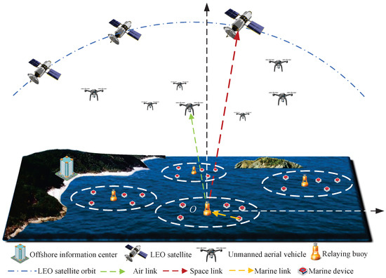
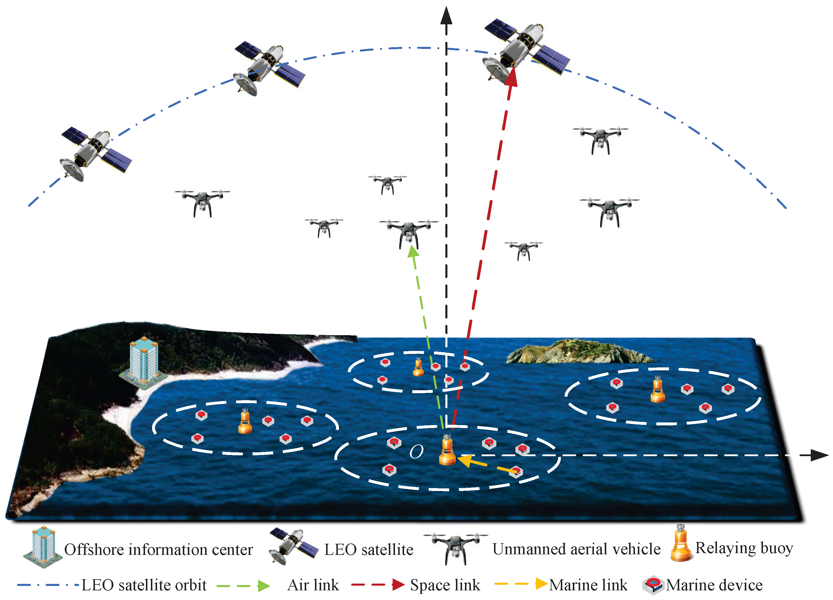
Let us consider an LSU-MIoT network deployed far from the coastline, comprising multiple relaying buoys (RBs) and marine devices (MDs) in the marine layer, several hovering UAVs in the air layer, and a LEO satellite constellation in the space layer, as shown in Figure 1. In the marine layer, MDs are responsible for collecting marine data and transmitting it to RBs. According to prior studies [3], the spatial locations of RBs and MDs distributed over the sea surface within the target area can be characterized using a Matérn cluster process. Specifically, the distributions of RBs and MDs are represented by parents and offspring children, where RBs act as cluster centers (parents) and MDs correspond to cluster members (offspring children). The distribution of RBs follows a two-dimensional HPPP with density ${\lambda }_{\mathrm{RB}}$, denoted as ${\Phi }_{\mathrm{RB}}=\left\{x_0,x_1,\dots ,x_W\right\}$. The distribution of $N_{\mathrm{M}}$ MDs is denoted as ${\Phi }_{\mathrm{MD}}=\left\{y_0,y_1,\dots ,y_{N_{\mathrm{M}}}\right\}$, where the MDs within each cluster are uniformly distributed within a radius $r_{\mathrm{clu}}$ around the cluster center RB. In each cluster, MDs are indexed according to their distance to their serving RB, designating each of them as the $k^{\mathrm{th}}\left(1\le k\le N_{\mathrm{M}}\right)$ MD, from the closest to the farthest. Correspondingly, the distance between the $k^{\mathrm{th}}$ MD and the serving RB is denoted as $R_{\mathrm{MB},k}$. In the air layer, UAVs hover at a fixed height over the sea surface and the distribution of UAVs follows an HPPP with density ${\lambda }_{\mathrm{UAV}}$, denoted as ${\Phi }_{\mathrm{UAV}}$. They are responsible for receiving the collected marine data while hovering above the sea surface and periodically delivering the data to the offshore information center by flight. The offshore information center is deployed near the coastline and acts as the destination node. It can obtain the marine data brought back by UAVs and connect to the backbone network. In the space layer, LEO satellites are uniformly distributed on a sphere at a certain altitude above the Earth’s surface, forming a spherical Poisson point process (SPPP) denoted as ${\Phi }_{\mathrm{LEO}}$ with density ${\lambda }_{\mathrm{S}}$. Each satellite is equipped with a directional antenna whose main beam is oriented toward the Earth’s center, enabling it to receive marine data collected from RBs during its overpass within the service footprint and relay the marine data to the backbone network. The network is analyzed in a snapshot manner, where the positions of LEO satellites and UAVs are assumed to be fixed during one transmission interval.

We employ three types of channel links to facilitate marine data transmission, including the marine, air, and space links. In the marine link, each cluster is allocated an individual channel operating at 700 MHz to support signal transmission from MDs to their cluster head. The air link comprises a 2.4 GHz channel to transmit signals from RBs to UAVs. Moreover, the space link employs a Ka-band channel for signal transmissions from RBs to LEO satellites.

In the LSU-MIoT network, marine data is generally categorized into regular and emergency data. Regular data include environmental measurements, e.g., temperature, salinity, and pH, within normal thresholds and are considered delay-tolerant. In contrast, emergency data comprise out-of-range environmental measurements and maritime incident reports, and are characterized as delay-sensitive. When an MD collects a regular data packet in a typical cluster, we establish a three-dimensional Cartesian coordinate system with the original point, i.e., $O\left(0,0,0\right)$ at the RB in the typical cluster, x-axis points in any direction from the origin within the sea surface, the y-axis is perpendicular to the x-axis and lies on the sea surface, and the z-axis is perpendicular to both the x-axis and y-axis. Then, UAVs are located on a two-dimensional plane at a height of $h_{\mathrm{UAV}}$ from the sea surface. The intersection point between the two-dimensional plane and the z-axis is denoted as $O^{\prime }\left(0,0,h_{\mathrm{UAV}}\right)$. The horizontal distance between point $O^{\prime }$ and its nearest UAV is denoted by $R_{\mathrm{BU}}$, where the nearest UAV is referred to as the serving UAV. In contrast, when an MD generates an emergency data packet in a typical cluster, we establish a three-dimensional Cartesian coordinate system with the original point set at the Earth’s center. Without loss of generality and according to Slivnyak’s theorem [18], the RB in the typical cluster is placed at the observation point $\left(0,0,r_{\mathrm{e}}\right)$, where $r_{\mathrm{e}}$ denotes the Earth’s radius. The vector from the origin to the North Pole is defined as the z-axis, and the vector in the Earth’s equatorial plane is defined as the y-axis. The x-axis direction vector is perpendicular to both axes y and z. LEO satellites are located on a sphere with radius $r_{\mathrm{S}}=r_{\mathrm{e}}+r_{\min }$, where $r_{\min }$ denotes the constellation altitude. The maximum possible distance between the RB and a LEO satellite over its horizon, known as the visible distance, is represented by $r_{\max }=\sqrt{2r_{\mathrm{e}}{r}_{\min }+r_{\min }^2}$ [19] and the LEO satellites over the horizon are referred to as visible satellites, forming a subset of LEO satellites, denoted as ${\Phi }_{\mathrm{vis}}$. Accordingly, the distance between the RB and its nearest LEO satellite is denoted as $R_{\mathrm{BS}}$, where the nearest satellite is referred to as the serving satellite. Moreover, other mathematical notions in the LSU-MIoT network are listed in

Table 1. Tables of Mathematical Notions.

Notions	Descriptions
${\Phi }_{\mathrm{MD}};{\Phi }_{\mathrm{RB}};{\Phi }_{\mathrm{out}}$	Set of MDs; Set of RBs; Set of interfering MDs
${\Phi }_{\mathrm{UAV}};{\Phi }_{\mathrm{LEO}};{\Phi }_{\mathrm{vis}}$	Set of UAVs; Set of LEO satellites; Set of visible satellites
$r_{\mathrm{e}};r_{\min };r_{\max };r_{\mathrm{S}}$	Earth radius; Constellation altitude; The visible distance; Constellation radius
$r_{\mathrm{clu}};h_{\mathrm{UAV}}$	Cluster radius; Height of UAVs
$R_{\mathrm{MB},k};R_{\mathrm{out}};R_{\mathrm{BU}};R_{\mathrm{BS}}$	Distance from the $k^{\mathrm{th}}$ MD to the serving RB; Distance from the interfering MD to the serving RB; Distance from the RB to the serving UAV; Distance from the RB to the serving LEO satellites
${\lambda }_{\mathrm{m}};{\lambda }_{\mathrm{a}};{\lambda }_{\mathrm{s}}$	Carrier wavelength in the marine link; Carrier wavelength in the air link; Carrier wavelength in the space link;
$N_{\mathrm{M}};{\lambda }_{\mathrm{UAV}};{\lambda }_{\mathrm{S}}$	The number of MDs per cluster; The density of UAVs; The density of LEO satellites
$h_{\mathrm{t},\mathrm{MD}};h_{\mathrm{r},\mathrm{RB}};h_{\mathrm{t},\mathrm{RB}};h_{\mathrm{r},\mathrm{U}}$	Transmit antenna height of the MD; Receive antenna height of the RB; Transmit antenna height of the RB; Receive antenna height of the UAV
$m;K_{\mathrm{Ri}};b;m_{\mathrm{s}};{\Omega }_{\mathrm{s}}$	Nakagami-m parameter in the marine link; Rician K factor; Half Average power of the scatter multi-path components; Nakagami-m parameter in the SR fading; average power of LoS component
$p_{\mathrm{M}};p_{\mathrm{B}}$	Transmit power of the MD; Transmit power of the RB
$G_{\mathrm{MB}};G_{\mathrm{BU}};G_{\mathrm{BS}}$	Antenna gain from the MD and RB; Antenna gain from the RB to the UAV; Antenna gain from the RB to the LEO satellite
$H_{\mathrm{MB},k};H_{\mathrm{BU}};H_{\mathrm{BS}}$	Channel coefficient from the $k^{\mathrm{th}}$ MD to the serving RB; Channel coefficient from the RB to the serving UAV; Channel coefficient from the RB to the serving LEO satellite
${\sigma }_{\mathrm{MB}}^2;{\sigma }_{\mathrm{BU}}^2;{\sigma }_{\mathrm{BS}}^2$	Additive noise power in the marine link; Additive noise power in the air link; Additive noise power in the space link
$B_{\mathrm{m}};B_{\mathrm{s}}$	Bandwidth of the marine link; Bandwidth of the space link
$f_{\mathrm{m}};f_{\mathrm{a}};f_{\mathrm{s}}$	Carrier frequency in the marine link; Carrier frequency in the air link; Carrier frequency in the space link
$\omega ;\Delta T;N_{\mathrm{q}}$	Length of data packet; Time duration per time slot; The number of time slots an MD should wait under the TDMA scheme
${\mathrm{SNR}}_{\mathrm{MB},k}^{\mathrm{T}};{\mathrm{SINR}}_{\mathrm{MB},k}^{\mathrm{N}}$	Received SNR from the $k^{\mathrm{th}}$ MD to the serving RB under the TDMA scheme; Received SINR from the $k^{\mathrm{th}}$ MD to the serving RB under the NOMA scheme
$\mathrm{SN}{\mathrm{R}}_{\mathrm{BU}};\mathrm{SN}{\mathrm{R}}_{\mathrm{BS}}$	Received SNR at the serving UAV; Received SNR at the serving satellite
$P_{\mathrm{re}}^{\mathrm{T}}\left(\tau \right);P_{\mathrm{em}}^{\mathrm{T}}\left(\tau \right);P_k^{\mathrm{T}}\left(\tau \right)$	Transmission success probability of the regular data under the TDMA scheme; Transmission success probability of the emergency data under the TDMA scheme; Transmission success probability from the $k^{\mathrm{th}}$ MD to the serving RB under the TDMA scheme
$P_{\mathrm{re}}^{\mathrm{N}}\left(\tau \right);P_{\mathrm{em}}^{\mathrm{N}}\left(\tau \right);P_k^{\mathrm{N}}\left(\tau \right)$	Transmission success probability of the regular data under the NOMA scheme; Transmission success probability of the emergency data under the NOMA scheme; Transmission success probability from the $k^{\mathrm{th}}$ MD to the serving RB under the NOMA scheme;
$P_{\mathrm{BU}}\left(\tau \right);P_{\mathrm{BS}}^{\mathrm{T}}\left(\tau \right)$	Transmission success probability from the RB to the serving UAV; Transmission success probability from the RB to the serving satellite
$C_k^{\mathrm{T}};C_k^{\mathrm{N}}$	Transmission rate capacity from the $k^{\mathrm{th}}$ MD to the serving RB under the TDMA scheme; Transmission rate capacity from the $k^{\mathrm{th}}$ MD to the serving RB under the NOMA scheme
$D_{\mathrm{em}}^{\mathrm{T}};D_k^{\mathrm{T}};D_q$	End-to-end delay of emergency data under the TDMA scheme; Transmission delay from the $k^{\mathrm{th}}$ MD to the serving RB under the TDMA scheme; Queuing delay
$D_{\mathrm{em}}^{\mathrm{N}};D_k^{\mathrm{N}};D_{\mathrm{BS}}$	End-to-end delay of emergency data under the NOMA scheme; Transmission delay from the $k^{\mathrm{th}}$ MD to the serving RB under the NOMA scheme; Transmission delay from the RB to the serving satellite

.

2.2. Data Transmission Scheme

In the LSU-MIoT network, we consider two data transmission schemes for supporting marine data acquisition from MDs to the offshore information center.

2.2.1. Time Division Multiple Access (TDMA) Scheme

In this scheme, the channel for each cluster in the marine link is divided into multiple time slots according to the number of MDs within each cluster. The TDMA scheme consists of two phases, namely the marine transmission phase and the relaying phase. For regular data transmission, during the marine transmission phase, $K\left(K\le N_{\mathrm{M}}\right)$ MDs sequentially transmit their collected data to the cluster head (marked as the serving RB) over the marine link in their assigned time slots. In the subsequent relaying phase, the serving RB forwards the aggregated data to the serving UAV. After completing multiple cycles of these two phases, UAVs periodically return to the shore to deliver the collected data to the offshore information center. For emergency data transmission, in the marine transmission phase, when the $k^{\mathrm{th}}$ MD collects an emergency data, it waits until its allocated time slot arrives, and then transmits the emergency data to the serving RB. Then, in the relaying phase, the serving RB immediately forwards the emergency data to the serving satellite. Since LEO satellites are connected to the backbone network, the offshore information center can promptly obtain the emergency data through the backbone network.

2.2.2. Non-Orthogonal Multiple Access (NOMA) Scheme

In the NOMA scheme, all MDs within a cluster simultaneously transmit their collected data to the RB over the shared channel in the marine link. For ease of presentation, the received signal powers are ordered consistently with the MD ordering in each cluster [20]. By employing perfect successive interference cancellation technology, when decoding the signal from the $k^{\mathrm{th}}$ MD, the RB sequentially decodes and eliminates the interference from the $k-1$ strong interfering MDs, such that only the signals from MDs located farther from the RB than the $k^{\mathrm{th}}$ MD within each cluster are regarded as interference [21]. The corresponding MDs treated as interfering MDs is denoted as ${\Phi }_{\mathrm{out}}=\left\{y_{k+1},\dots ,y_{N_{\mathrm{M}}}\right\}$. Except for the multiple access mechanism, the subsequent transmission procedures in the marine transmission and relaying phases are identical to those described for the TDMA scheme.

2.3. Channel Model

In the marine, air, and space links, we employ large-scale attenuation and small-scale fading to represent the propagation characteristics in the LSU-MIoT network.

2.3.1. Path Loss Model

In the marine and air layers, since signal propagation encounters multiple factors such as reflections and refraction, we employ a two-ray model, which is widely recognized to effectively reflect the practice radio propagation environment over the sea surface. The two-ray path loss model is expressed as [22,23]

$$L\left(R\right)={\left({\displaystyle \frac{{\lambda }_c}{4\pi R}}\right)}^2{\left(2sin\left({\displaystyle \frac{2\pi }{{\lambda }_c}}{\displaystyle \frac{h_{\mathrm{t}}{h}_{\mathrm{r}}}{R}}\right)\right)}^2,$$

(1)

where R is the distance between the transmitter and the receiver, $h_{\mathrm{t}}$ and $h_{\mathrm{r}}$ are the transmitter and receiver antenna heights, ${\lambda }_c$ denotes the carrier wavelength.

For the space link, we utilize a distance-dependent power path loss model to characterize the signal power loss between the LEO satellite and the RB, which is expressed as [24]

$$L\left(R_{\mathrm{BS}}\right)={\left({\displaystyle \frac{c}{4\pi f_c}}\right)}^2{R}_{\mathrm{BS}}^{-\alpha },$$

(2)

where $R_{\mathrm{BS}}$ is the distance between the RB and LEO satellite, c is the speed of light, $f_c$ is the carrier frequency of the signal and $\alpha$ denotes the path loss exponent.

2.3.2. Fading Model

For the marine link, we employ the Nakagami-m fading model in the channel coefficient H to represent signal attenuation caused by fluctuating waves over the sea surface. Accordingly, the corresponding channel gain ${\left|H\right|}^2$ follows Gamma distribution with shape and scale parameters $\left(m,1/m\right)$, whose cumulative distribution function (CDF) is expressed as [25]

$$F_{|H{|}^2}\left(x\right)={\displaystyle \frac{\gamma \left(m,mx\right)}{\Gamma \left(m\right)}},$$

(3)

where m is the Nakagami parameter, and $\Gamma \left(·\right)$ and $\gamma \left(·,·\right)$ are the Gamma function and the lower incomplete Gamma function, respectively. Accordingly, the probability density function (PDF) of channel gain ${\left|H\right|}^2$ under the Gamma distribution is expressed as

$$f_{{\left|H\right|}^2}\left(x\right)={\displaystyle \frac{x^{m-1}{\mathrm{e}}^{-\frac{x}{m}}}{m^m\Gamma \left(m\right)}}.$$

(4)

For the air link, due to the dominant line-of-sight (LoS) component, the Rician fading model is employed to characterize signal propagation between the RB and the UAV, whose CDF of channel gain ${\left|H\right|}^2$ is given by [26]

$$F_{{\left|H\right|}^2}\left(x\right)=1-{\mathcal{Q}}_1\left(\sqrt{2K_{\mathrm{R}}},\sqrt{2\left(K_{\mathrm{R}}+1\right)x}\right),$$

(5)

where $K_{\mathrm{R}}$ denotes the Rician K factor, which is defined as the ratio of the power of the LoS component to the scattered components, and $Q_1\left(a,b\right)\stackrel{\Delta }{=}{\int }_b^{\infty }x{e}^{-{\displaystyle \frac{a^2+x^2}{2}}}{I}_0\left(ax\right)dx$ is the Marcum Q-function of the first kind.

For the space layer, we employ the shadowed Rician (SR) fading model to represent the channel gain between the LEO satellite and the RB, which is widely recognized to describe the propagation character in satellite communications, and the CDF of the channel gain ${\left|H\right|}^2$ under the SR fading is expressed as [12]

$$\begin{array}{c}\hfill F_{|H{|}^2}(x)=1-\mu \sum _{n=0}^{m_{\mathrm{s}}-1}{\displaystyle \frac{{(1-m_{\mathrm{s}})}_n{(-\delta )}^n}{{(n!)}^2}}\sum _{l=0}^n{\displaystyle \frac{n!}{l!}}{(\beta -\delta )}^{-(n+1-l)}{x}^l{\mathrm{e}}^{-(\beta -\delta )x},\end{array}$$

(6)

where $\mu ={\displaystyle \frac{1}{2b}}{\left({\displaystyle \frac{2b{m}_{\mathrm{s}}}{2b{m}_{\mathrm{s}}+{\Omega }_{\mathrm{s}}}}\right)}^{m_{\mathrm{s}}}$, $\delta ={\displaystyle \frac{1}{2b}}\left({\displaystyle \frac{{\Omega }_{\mathrm{s}}}{2b{m}_{\mathrm{s}}+{\Omega }_{\mathrm{s}}}}\right)$, $\beta ={\displaystyle \frac{1}{2b}}$ with ${\Omega }_{\mathrm{s}}$, $m_{\mathrm{s}}$ and b being the average power of the LoS component, the Nakagami parameter in the SR fading model, and the half average power of the scattered multi-path components, respectively. In addition, ${\left(x\right)}_n=x\left(x+1\right)\dots \left(x+n-1\right)$ is the Pochhammer symbol. Accordingly, the PDF of the channel gain ${\left|H\right|}^2$ is expressed as [27]

$$\begin{array}{c}\hfill f_{{\left|H\right|}^2}\left(x\right)=\mu \sum _{n=0}^{m_{\mathrm{s}}-1}{\displaystyle \frac{{\left(1-m_{\mathrm{s}}\right)}_n{\left(-\delta \right)}^n}{{\left(n!\right)}^2}}{x}^n{\mathrm{e}}^{-\left(\beta -\delta \right)x}.\end{array}$$

(7)

3. Peformance Analysis

In this section, we derive analytical expressions of the transmission success probability and the end-to-end delay for the regular and emergency data under the TDMA and NOMA schemes, respectively.

3.1. Preliminaries

To derive analytical expressions of the LSU-MIoT network in the subsequent sections, we employ some preliminary Lemmas as follows [18,20,28].

Lemma 1.

The PDF of distance $R_{\mathrm{MB},k}$ from the $k^{\mathrm{th}}$ MD to the serving RB is given by

$$f_{R_{\mathrm{MB},k}}\left(r_{\mathrm{MB},k}\right)={\displaystyle \frac{2r_{\mathrm{MB},k}^{2k-1}{\left(1-\frac{r_{\mathrm{MB},k}^2}{r_{\mathrm{clu}}^2}\right)}^{N_{\mathrm{M}}-k}}{r_{\mathrm{clu}}^{2k}B\left(k,N_{\mathrm{M}}-k+1\right)}},$$

(8)

where $N_{\mathrm{M}}$ is the number of MDs per cluster, k is the MD index, $r_{\mathrm{clu}}$ is the cluster radius, and $B(z_1,z_2)={\int }_0^1{t}^{z_1-1}{(1-t)}^{z_2-1}dt$ denotes the Euler Beta function.

Lemma 2.

Conditioned on signal transmissions from the $k^{\mathrm{th}}$ MD to the serving RB, when employing the NOMA scheme, interfering MDs are located beyond the $k^{\mathrm{th}}$ MD within the cluster in set ${\Phi }_{\mathrm{out}}$. Therefore, the PDF of distance from any MD in the set ${\Phi }_{\mathrm{out}}$ to the serving RB can be expressed as

$$f_{R_{\mathrm{out}}|R_{\mathrm{MB},k}}\left(r_{\mathrm{out}}|r_{\mathrm{MB},k}\right)={\displaystyle \frac{2r_{\mathrm{out}}}{r_{\mathrm{clu}}^2-R_{\mathrm{MB},k}^2}},r_{\mathrm{MB},k}<r_{\mathrm{out}}\le r_{\mathrm{clu}},$$

(9)

where $R_{\mathrm{out}}$ is the distance from any MD in the set ${\Phi }_{\mathrm{out}}$ and the serving RB, where $r_{\mathrm{out}}$ and $r_{\mathrm{MB},k}$ denote the realization of variable $R_{\mathrm{out}}$ and $R_{\mathrm{MB},k}$.

Lemma 3.

The PDF of the horizontal distance between the RB and the serving UAV is expressed as

$$f_{R_{\mathrm{BU}}}\left(r_{\mathrm{BU}}\right)=2\pi {\lambda }_{\mathrm{UAV}}{r}_{\mathrm{BU}}{e}^{-{\lambda }_{\mathrm{UAV}}\pi r_{\mathrm{BU}}^2},$$

(10)

where ${\lambda }_{\mathrm{UAV}}$ denotes the density of UAVs.

Lemma 4.

The PDF of distance $R_{\mathrm{BS}}$ is given by

$$f_{R_{\mathrm{BS}}|{\Phi }_{\mathrm{vis}}>0}\left(r_{\mathrm{BS}}\right)=2\pi {\lambda }_{\mathrm{S}}{\displaystyle \frac{r_{\mathrm{S}}}{r_{\mathrm{e}}}}{\displaystyle \frac{e^{{\lambda }_{\mathrm{s}}\pi \frac{r_{\mathrm{S}}}{r_{\mathrm{e}}}\left(r_{\mathrm{S}}^2-r_{\mathrm{e}}^2\right)}}{e^{2\pi {\lambda }_{\mathrm{s}}{r}_{\mathrm{S}}{r}_{\min }}-1}}{r}_{\mathrm{BS}}{e}^{-{\lambda }_{\mathrm{s}}\pi {\displaystyle \frac{r_{\mathrm{S}}}{r_{\mathrm{e}}}}{r}_{\mathrm{BS}}^2},r_{\min }\le r_{\mathrm{BS}}\le r_{\max },$$

(11)

where the condition ${\Phi }_{\mathrm{vis}}>0$ implies the presence of at least one LEO satellite above the horizon.

3.2. Transmission Success Probability

The performance measure of the transmission success probability for an individual MD over a particular link is defined as the received SNR (or SINR) surpassing a predefined threshold, i.e., $P\left(\tau \right)\stackrel{\Delta }{=}\mathbb{P}\left(\mathrm{SNR}>\tau \right)$ (or $P\left(\tau \right)\stackrel{\Delta }{=}\mathbb{P}\left(\mathrm{SINR}>\tau \right)$). Under the TDMA or NOMA scheme, the transmission is considered as successful when all the MDs within a cluster successfully transmit their data to the UAV through the RB.

3.2.1. Transmission Success Probability Under the TDMA Scheme

In the LSU-MIoT network under the TDMA scheme, signal transmissions occur only during the time slot allocated to each MD, and thus there will be no interference generated.

For the marine link, under the TDMA scheme, the received SNR from the $k^{\mathrm{th}}$ MD to the serving RB is expressed as

$${\mathrm{SNR}}_{\mathrm{MB},k}^{\mathrm{T}}={\displaystyle \frac{p_{\mathrm{M}}{G}_{\mathrm{MB}}{L}_{\mathrm{MB}}(R_{\mathrm{MB},k})|H_{\mathrm{MB},k}{|}^2}{{\sigma }_{\mathrm{MB}}^2}},$$

(12)

where $p_{\mathrm{M}}$ is the transmit power of the MD, $G_{\mathrm{MB}}$ is the antenna gain encompassing both the transmitter and receiver, ${\sigma }_{\mathrm{MB}}^2$ is the received power of the additive noise in the marine link, $L_{\mathrm{MB}}(R_{\mathrm{MB},k})$ is the path-loss model with $R_{\mathrm{MB},k}$ denoting the distance between the $k^{\mathrm{th}}$ MD and the serving RB, employing the two-ray path loss model, and $H_{\mathrm{MB},k}$ represents the channel coefficient, employing the Nakagami-m fading model.

For the air link, the received SNR in the uplink from the RB to the serving UAV is expressed as

$${\mathrm{SNR}}_{\mathrm{BU}}={\displaystyle \frac{p_{\mathrm{B}}{G}_{\mathrm{BU}}{L}_{\mathrm{BU}}\left(R_{\mathrm{BU}}\right)|H_{\mathrm{BU}}{|}^2}{{\sigma }_{\mathrm{BU}}^2}},$$

(13)

where $p_{\mathrm{B}}$ is the transmit power of the RB, $G_{\mathrm{BU}}$ denotes the antenna gain from the RB to the UAV, $L_{\mathrm{BU}}\left(R_{\mathrm{BU}}\right)$ employs the two-ray path loss model with $R_{\mathrm{BU}}$ denoting the distance between the RB and the serving UAV, ${\sigma }_{\mathrm{BU}}^2$ denotes the received power of the additive noise in the air link, and $|H_{\mathrm{BU}}{|}^2$ is the channel gain in the air link, employing the Rician fading model.

The transmission success probability of the regular data under the TDMA scheme is expressed as the joint distribution that all the SNRs from K MDs to the serving RB over the marine link and the SNR from the RB to the serving UAV over the air link are above the threshold, which is shown as

$$P_{\mathrm{re}}^{\mathrm{T}}\left(\tau \right)\stackrel{\Delta }{=}\mathbb{P}\left(\underset{k=1}{\overset{K}{\cap }}\left\{{\mathrm{SNR}}_{\mathrm{MB},k}^{\mathrm{T}}>\tau \right\},\mathrm{SN}{\mathrm{R}}_{\mathrm{BU}}>\tau \right),$$

(14)

where $\mathrm{SN}{\mathrm{R}}_{\mathrm{MB},k}^{\mathrm{T}}$ denotes the received SNR from the $k^{\mathrm{th}}$ MD to the serving RB under the TDMA scheme and $\mathrm{SN}{\mathrm{R}}_{\mathrm{BU}}$ is the received SNR at the serving UAV.

For regular data transmission under the TDMA scheme, the independence between the marine and air links allows the joint distribution to be simplified to the product of the transmission success probabilities of the marine and the air links.

Theorem 1.

Under the TDMA scheme, the transmission success probability of the regular data is expressed as

$$P_{\mathrm{re}}^{\mathrm{T}}\left(\tau \right)=P_{\mathrm{BU}}\left(\tau \right)\prod _{k=1}^K{P}_k^{\mathrm{T}}\left(\tau \right),$$

(15)

where $P_k^{\mathrm{T}}\left(\tau \right)$ is the transmission success probability from the $k^{\mathrm{th}}$ MD to the serving RB under the TDMA scheme, which is expressed as

$$P_k^{\mathrm{T}}\left(\tau \right)={\int }_0^{r_{\mathrm{clu}}}\tilde{\Gamma }\left(m,{\displaystyle \frac{m\tau {\sigma }_{\mathrm{MB}}^2{\left(4\pi r_{\mathrm{MB},k}\right)}^2}{p_{\mathrm{M}}{G}_{\mathrm{MB}}{\left(2{\lambda }_{\mathrm{m}}sin\left(\frac{2\pi }{{\lambda }_{\mathrm{m}}}\frac{h_{\mathrm{t},\mathrm{MD}}{h}_{\mathrm{r},\mathrm{RB}}}{r_{\mathrm{MB},k}}\right)\right)}^2}}\right)f_{R_{\mathrm{MB},k}}\left(r_{\mathrm{MB},k}\right)d{r}_{\mathrm{MB},k},$$

(16)

where $\tilde{\Gamma }\left(·,·\right)={\displaystyle \frac{\Gamma \left(·,·\right)}{\Gamma \left(·\right)}}$ is the regularized gamma function, ${\lambda }_{\mathrm{m}}$ is the carrier wavelength in the marine link, $h_{\mathrm{t},\mathrm{MD}}$ and $h_{\mathrm{r},\mathrm{RB}}$ are the antenna heights at the transmitter (MD) and receiver (RB), respectively, and $f_{R_{\mathrm{MB},k}}\left(r_{\mathrm{MB},k}\right)$ is the PDF of the distance between the $k^{\mathrm{th}}$ MD and the serving RB, given in Lemma 1, $P_{\mathrm{BU}}\left(\tau \right)$ is the transmission success probability from the RB to the serving UAV, which is expressed as

$$P_{\mathrm{BU}}\left(\tau \right)={\int }_0^{\infty }{Q}_1\left(\sqrt{2K_{\mathrm{R}}},{\displaystyle \frac{\sqrt{2\left(K_{\mathrm{R}}+1\right)}\tau {\sigma }_{\mathrm{BU}}^2{\left(4\pi r_{\mathrm{BU}}\right)}^2}{p_{\mathrm{B}}{\mathrm{G}}_{\mathrm{BU}}{\left(2{\lambda }_{\mathrm{a}}sin\left(\frac{2\pi }{{\lambda }_{\mathrm{a}}}\frac{h_{\mathrm{t},\mathrm{RB}}{h}_{\mathrm{r},\mathrm{U}}}{{\left(r_{\mathrm{BU}}^2+h_{\mathrm{UAV}}^2\right)}^{\frac{1}{2}}}\right)\right)}^2}}\right)f_{R_{\mathrm{BU}}}\left(r_{\mathrm{BU}}\right)d{r}_{\mathrm{BU}},$$

(17)

where ${\lambda }_{\mathrm{a}}$ is the carrier wavelength in the air link, $h_{\mathrm{t},\mathrm{RB}}$ and $h_{\mathrm{r},\mathrm{U}}$ are the antenna heights at the transmitter (RB) and receiver (UAV), respectively, and $f_{R_{\mathrm{BU}}}\left(r_{\mathrm{BU}}\right)$ is the PDF of the distance between the RB and the serving UAV, given in Lemma 3.

Proof of Theorem 1.

To obtain (16), we start with the definition of the transmission success probability from the $k^{\mathrm{th}}$ MD to the serving RB under the TDMA scheme, which is expressed as

$$\begin{array}{cc}\hfill P_k^{\mathrm{T}}\left(\tau \right)& \stackrel{\Delta }{=}\mathbb{P}\left(\mathrm{SN}{\mathrm{R}}_{\mathrm{MB},k}^{\mathrm{T}}>\tau \right)\hfill \\ \hfill & =\mathbb{P}\left({\displaystyle \frac{p_{\mathrm{M}}{G}_{\mathrm{MB}}{\left|H_{\mathrm{MB},k}\right|}^2{L}_{\mathrm{MB}}\left(R_{\mathrm{MB},k}\right)}{{\sigma }_{\mathrm{MB}}^2}}>\tau \right)\hfill \\ \hfill & =\mathbb{P}\left({\left|H_{\mathrm{MB},k}\right|}^2>{\displaystyle \frac{\tau {\sigma }_{\mathrm{MB}}^2}{p_{\mathrm{M}}{G}_{\mathrm{MB}}{L}_{\mathrm{MB}}\left(R_{\mathrm{MB},k}\right)}}\right)\hfill \\ \hfill & \underline{\underline{\left(a\right)}}\tilde{\Gamma }\left(m,{\displaystyle \frac{m\tau {\sigma }_{\mathrm{MB}}^2}{p_{\mathrm{M}}{G}_{\mathrm{MB}}{L}_{\mathrm{MB}}\left(R_{\mathrm{MB},k}\right)}}\right)\hfill \\ \hfill & \underline{\underline{\left(b\right)}}{\int }_0^{r_{\mathrm{clu}}}\tilde{\Gamma }\left(m,{\displaystyle \frac{m\tau {\sigma }_{\mathrm{MB}}^2{\left(4\pi r_{\mathrm{MB},k}\right)}^2}{p_{\mathrm{M}}{G}_{\mathrm{MB}}{\left(2{\lambda }_{\mathrm{m}}sin\left(\frac{2\pi }{{\lambda }_{\mathrm{m}}}\frac{h_{\mathrm{t},\mathrm{MD}}{h}_{\mathrm{r},\mathrm{RB}}}{r_{\mathrm{MB},k}}\right)\right)}^2}}\right)f_{R_{\mathrm{MB},k}}\left(r_{\mathrm{MB},k}\right)d{r}_{\mathrm{MB},k},\hfill \end{array}$$

(18)

where $\left(a\right)$ is obtained using the complementary CDF (CCDF) of the Gamma distribution, $\left(b\right)$ is the average of the distance between the $k^{\mathrm{th}}$ MD and the serving RB using Lemma 1.

Similarly, to obtain (17), according to the definition of the transmission success probability from the RB to the serving UAV, which is given by

$$\begin{array}{cc}\hfill P_{\mathrm{BU}}\left(\tau \right)& \stackrel{\Delta }{=}\mathbb{P}\left(\mathrm{SN}{\mathrm{R}}_{\mathrm{BU}}>\tau \right)\hfill \\ \hfill & =\mathbb{P}\left({\displaystyle \frac{p_{\mathrm{B}}{\mathrm{G}}_{\mathrm{BU}}{L}_{\mathrm{BU}}\left(R_{\mathrm{BU}}\right){\left|H_{\mathrm{BU}}\right|}^2}{{\sigma }_{\mathrm{BU}}^2}}>\tau \right)\hfill \\ \hfill & =\mathbb{P}\left({\left|H_{\mathrm{BU}}\right|}^2>{\displaystyle \frac{\tau {\sigma }_{\mathrm{BU}}^2}{p_{\mathrm{B}}{\mathrm{G}}_{\mathrm{BU}}{L}_{\mathrm{BU}}\left(R_{\mathrm{BU}}\right)}}\right)\hfill \\ \hfill & \underline{\underline{(a)}}{Q}_1\left(\sqrt{2K_{\mathrm{R}}},{\displaystyle \frac{\sqrt{2\left(K_{\mathrm{R}}+1\right)}\tau {\sigma }_{\mathrm{BU}}^2}{p_{\mathrm{B}}{\mathrm{G}}_{\mathrm{BU}}{L}_{\mathrm{BU}}\left(R_{\mathrm{BU}}\right)}}\right)\hfill \\ \hfill & \underline{\underline{(b)}}{\int }_0^{\infty }{Q}_1\left(\sqrt{2K_{\mathrm{R}}},{\displaystyle \frac{\sqrt{2\left(K_{\mathrm{R}}+1\right)}\tau {\sigma }_{\mathrm{BU}}^2{\left(4\pi r_{\mathrm{BU}}\right)}^2}{p_{\mathrm{B}}{\mathrm{G}}_{\mathrm{BU}}{\left(2{\lambda }_{\mathrm{a}}sin\left(\frac{2\pi }{{\lambda }_{\mathrm{a}}}\frac{h_{\mathrm{t},\mathrm{RB}}{h}_{\mathrm{r},\mathrm{U}}}{{\left(r_{\mathrm{BU}}^2+h_{\mathrm{UAV}}^2\right)}^{\frac{1}{2}}}\right)\right)}^2}}\right)f_{R_{\mathrm{BU}}}\left(r_{\mathrm{BU}}\right)d{r}_{\mathrm{BU}},\hfill \end{array}$$

(19)

where $\left(a\right)$ follows from the CCDF of the Rician fading and $\left(b\right)$ is obtained by substituting the expression of the two-ray model and averaging over the PDF of the distance between the $k^{\mathrm{th}}$ MD and its serving RB in Lemma 3. □

For emergency data, once it is collected by an MD (denoted as the $k^{\mathrm{th}}$ MD), the MD transmits it to its serving RB in the assigned slot. Given the importance of emergency data, the RB immediately forwards it to the serving LEO satellite via the space link, without waiting to batch it with other packets. Consequently, the transmission success probability of the emergency data is expressed as the product of the transmission success probability from the MD that carries the emergency data to the serving RB and that from the RB to the serving satellite. Without loss of generality, we denote the MD that carries the emergency data to the serving RB.

Theorem 2.

Under the TDMA scheme, the transmission success probability of the emergency data is expressed as

$$P_{\mathrm{em}}^{\mathrm{T}}\left(\tau \right)=P_k^{\mathrm{T}}\left(\tau \right)P_{\mathrm{BS}}\left(\tau \right),$$

(20)

where $P_k^{\mathrm{T}}\left(\tau \right)$ is the transmission success probability from the $k^{\mathrm{th}}$ MD to the serving RB under the TDMA scheme, which is given in (16), $P_{\mathrm{BS}}\left(\tau \right)$ is the transmission success probability from the RB to the serving satellite, which is expressed as

$$\begin{array}{cc}\hfill P_{\mathrm{BS}}(\tau )=& {\int }_{r_{\min }}^{r_{\max }}\mu \sum _{n=0}^{m_{\mathrm{s}}-1}{\displaystyle \frac{{(1-m_{\mathrm{s}})}_n{(-\delta )}^n}{{\left(n!\right)}^2}}\sum _{l=0}^n{\displaystyle \frac{n!}{l!}}{\left(\beta -\delta \right)}^{-(n+1-l)}{\left({\displaystyle \frac{\tau {\sigma }_{\mathrm{BS}}^2{\left(4\pi f_{\mathrm{s}}\right)}^2{r}_{\mathrm{BS}}^{\alpha }}{c^2{p}_{\mathrm{B}}{\mathrm{G}}_{\mathrm{BS}}}}\right)}^l\hfill \\ \hfill & \times {\mathrm{e}}^{-(\beta -\delta ){\displaystyle \frac{\tau {\sigma }_{\mathrm{BS}}^2{\left(4\pi f_{\mathrm{s}}\right)}^2{r}_{\mathrm{BS}}^{\alpha }}{c^2{p}_{\mathrm{B}}{\mathrm{G}}_{\mathrm{BS}}}}}{f}_{R_{\mathrm{BS}}|{\Phi }_{\mathrm{vis}}\left(\mathcal{A}\right)>0}\left(r_{\mathrm{BS}}\right)d{r}_{\mathrm{BS}},\hfill \end{array}$$

(21)

where $f_{\mathrm{s}}$ is the carrier frequency in the space link and $f_{R_{\mathrm{BS}}|{\Phi }_{\mathrm{vis}}\left(\mathcal{A}\right)>0}\left(r_{\mathrm{BS}}\right)$ is the PDF of $R_{\mathrm{BS}}$ in Lemma 4.

Proof of Theorem 2.

To obtain (21), we start with the definition of the transmission success probability of the emergency data from the RB to the serving LEO satellite, which can be expressed as

$$\begin{array}{cc}\hfill P_{\mathrm{BS}}\left(\tau \right)& \stackrel{\Delta }{=}\mathbb{P}\left(\mathrm{SN}{\mathrm{R}}_{\mathrm{BS}}>\tau \right)\hfill \\ \hfill & =\mathbb{P}\left({\displaystyle \frac{p_{\mathrm{B}}{\mathrm{G}}_{\mathrm{BS}}{L}_{\mathrm{BS}}\left(R_{\mathrm{BS}}\right){\left|H_{\mathrm{BS}}\right|}^2}{{\sigma }_{\mathrm{BS}}^2}}>\tau \right)\hfill \\ \hfill & =\mathbb{P}\left({\left|H_{\mathrm{BS}}\right|}^2>{\displaystyle \frac{\tau {\sigma }_{\mathrm{BS}}^2{\left(4\pi f_{\mathrm{s}}\right)}^2{R}_{\mathrm{BS}}^{\alpha }}{c^2{p}_{\mathrm{B}}{\mathrm{G}}_{\mathrm{BS}}}}\right)\hfill \\ \hfill & \underline{\underline{(a)}}\mu \sum _{n=0}^{m_{\mathrm{s}}-1}{\displaystyle \frac{{(1-m_{\mathrm{s}})}_n{(-\delta )}^n}{{\left(n!\right)}^2}}\sum _{l=0}^n{\displaystyle \frac{n!}{l!}}{\left(\beta -\delta \right)}^{-(n+1-l)}{\left({\displaystyle \frac{\tau {\sigma }_{\mathrm{BS}}^2{\left(4\pi f_{\mathrm{s}}\right)}^2{R}_{\mathrm{BS}}^{\alpha }}{c^2{p}_{\mathrm{B}}{\mathrm{G}}_{\mathrm{BS}}}}\right)}^l\hfill \\ \hfill & \times {\mathrm{e}}^{-(\beta -\delta ){\displaystyle \frac{\tau {\sigma }_{\mathrm{BS}}^2{\left(4\pi f_{\mathrm{s}}\right)}^2{R}_{\mathrm{BS}}^{\alpha }}{c^2{p}_{\mathrm{B}}{\mathrm{G}}_{\mathrm{BS}}}}}\hfill \\ \hfill & \underline{\underline{(b)}}{\int }_{r_{\min }}^{r_{\max }}\mu \sum _{n=0}^{m_{\mathrm{s}}-1}{\displaystyle \frac{{(1-m_{\mathrm{s}})}_n{(-\delta )}^n}{{\left(n!\right)}^2}}\sum _{l=0}^n{\displaystyle \frac{n!}{l!}}{\left(\beta -\delta \right)}^{-(n+1-l)}{\left({\displaystyle \frac{\tau {\sigma }_{\mathrm{BS}}^2{\left(4\pi f_{\mathrm{s}}\right)}^2{r}_{\mathrm{BS}}^{\alpha }}{c^2{p}_{\mathrm{B}}{\mathrm{G}}_{\mathrm{BS}}}}\right)}^l\hfill \\ \hfill & \times {\mathrm{e}}^{-(\beta -\delta ){\displaystyle \frac{\tau {\sigma }_{\mathrm{BS}}^2{\left(4\pi f_{\mathrm{s}}\right)}^2{r}_{\mathrm{BS}}^{\alpha }}{c^2{p}_{\mathrm{B}}{\mathrm{G}}_{\mathrm{BS}}}}}{f}_{R_{\mathrm{BS}}|{\Phi }_{\mathrm{vis}}\left(\mathcal{A}\right)>0}\left(r_{\mathrm{BS}}\right)d{r}_{\mathrm{BS}},\hfill \end{array}$$

(22)

where $\left(a\right)$ is obtained by employing the CCDF of the SR fading model and $\left(b\right)$ utilizes the PDF of distance $R_{\mathrm{BS}}$ in Lemma 4. □

3.2.2. Transmission Success Probability Under the NOMA Scheme

Under the NOMA scheme, signal transmissions is affected by interfering MDs due to sharing a common channel in each cluster. Consequently, the derivations of the transmission success probability under the NOMA scheme follow the same procedure as in the TDMA scheme, except for the marine link, where interference must be accounted for.

The received SINR from the $k^{\mathrm{th}}$ MD to the serving RB under the NOMA scheme is expressed as

$$\mathrm{SIN}{\mathrm{R}}_{\mathrm{MB},k}^{\mathrm{N}}={\displaystyle \frac{p_{\mathrm{M}}{G}_{\mathrm{MB}}{L}_{\mathrm{MB}}(R_{\mathrm{MB},k})|H_{\mathrm{MB},k}{|}^2}{I_{\mathrm{M}}+{\sigma }_{\mathrm{MB}}^2}},$$

(23)

where $I_{\mathrm{M}}$ denotes the cumulative power of interfering MDs received at the serving RB, which is defined as

$$\begin{array}{c}\hfill I_{\mathrm{M}}\stackrel{\Delta }{=}\sum _{y_i\in {\Phi }_{\mathrm{out}}}{p}_{\mathrm{M}}{G}_{\mathrm{M}}{\left|H_{\mathrm{MB},i}\right|}^2{L}_{\mathrm{MB}}(R_{\mathrm{MB},i}),\end{array}$$

(24)

where $H_{\mathrm{MB},i}$ is the channel coefficient from the $i^{\mathrm{th}}$ MD to the serving RB, which also employs the Nakagami-m fading model with $R_{\mathrm{MB},i}$ denoting the distance between the interfering MDs and the serving RB.

For the space link, the received SNR from the RB to the serving satellite is expressed as

$$\begin{array}{c}\hfill \mathrm{SN}{\mathrm{R}}_{\mathrm{BS}}={\displaystyle \frac{p_{\mathrm{B}}{G}_{\mathrm{BS}}{L}_{\mathrm{BS}}\left(R_{\mathrm{BS}}\right)|H_{\mathrm{BS}}{|}^2}{{\sigma }_{\mathrm{BS}}^2}},\end{array}$$

(25)

where $G_{\mathrm{BS}}$ denotes the combined transmit and receive antenna gains for the link from the RB to the LEO satellite, $L_{\mathrm{BS}}\left(R_{\mathrm{BS}}\right)$ represents the path loss model, employing the power path loss model model defined in (2) with $R_{\mathrm{BS}}$ denoting the distance between the RB and the serving satellite, and ${\sigma }_{\mathrm{BS}}^2$ denotes the received power of additive noise in the space link.

Theorem 3.

Under the NOMA scheme, the transmission success probability of the regular data is expressed as

$$P_{\mathrm{re}}^{\mathrm{N}}\left(\tau \right)=P_{\mathrm{BU}}\left(\tau \right)\prod _{k=1}^K{P}_k^{\mathrm{N}}\left(\tau \right),$$

(26)

where $P_{\mathrm{BU}}\left(\tau \right)$ is given in (17) and $P_k^{\mathrm{N}}\left(\tau \right)$ is the transmission success probability from the $k^{\mathrm{th}}$ MD to the serving RB under the NOMA scheme, which is expressed as

$$\begin{array}{cc}\hfill P_k^{\mathrm{N}}\left(\tau \right)& ={\int }_0^{r_{\mathrm{clu}}}\left(\sum _{n=1}^m\left(\begin{array}{c}m\\ n\end{array}\right){\left(-1\right)}^{n+1}exp\left(-{\displaystyle \frac{nm\beta {\sigma }_{\mathrm{MB}}^2\tau {\left(4\pi r_{\mathrm{MB},k}\right)}^2}{p_{\mathrm{M}}{G}_{\mathrm{MB}}{\left(2{\lambda }_{\mathrm{m}}sin\left(\frac{2\pi }{{\lambda }_{\mathrm{m}}}\frac{h_{\mathrm{t},\mathrm{MD}}{h}_{\mathrm{r},\mathrm{RB}}}{r_{\mathrm{MB},k}}\right)\right)}^2}}\right)\right.\hfill \\ \hfill & \times \left.{\mathcal{L}}_{I_{\mathrm{M}}}\left({\mathrm{s}}_1\right)\right)f_{R_{\mathrm{MB},k}}\left(r_{\mathrm{MB},k}\right)d{r}_{\mathrm{MB},k},\hfill \end{array}$$

(27)

where $s_1={\displaystyle \frac{n\beta m\tau {\left(4\pi r_{\mathrm{MB},k}\right)}^2}{p_{\mathrm{M}}{G}_{\mathrm{MB}}{\left(2{\lambda }_{\mathrm{m}}sin\left(\frac{2\pi }{{\lambda }_{\mathrm{m}}}\frac{h_{\mathrm{t},\mathrm{MD}}{h}_{\mathrm{r},\mathrm{RB}}}{r_{\mathrm{MB},k}}\right)\right)}^2}}$ and ${\mathcal{L}}_{I_{\mathrm{M}}}\left(s_1\right)$ denotes the Laplace transform of the cumulative power from interfering MDs, which is given by

$${\mathcal{L}}_{I_{\mathrm{M}}}\left(s_1\right)={\left({\int }_{r_k}^{r_{\mathrm{clu}}}{\displaystyle \frac{2r_{\mathrm{out}}}{\left(r_{\mathrm{clu}}^2-r_k^2\right)}}{\displaystyle \frac{1}{{\left(1+\frac{s_1{p}_{\mathrm{M}}{G}_{\mathrm{MB}}{\left(2{\lambda }_{\mathrm{m}}sin\left(\frac{2\pi }{{\lambda }_{\mathrm{m}}}\frac{h_{\mathrm{t},\mathrm{MD}}{h}_{\mathrm{r},\mathrm{RB}}}{r_{\mathrm{out}}}\right)\right)}^2}{m{\left(4\pi r_{\mathrm{out}}\right)}^2}\right)}^m}}d{r}_{\mathrm{out}}\right)}^{N_{\mathrm{M}}-k}.$$

(28)

Proof of Theorem 3.

To obtain (27), we start with the definition of transmission success probability under the NOMA scheme, which is expressed as

$$\begin{array}{cc}\hfill P_k^{\mathrm{N}}\left(\tau \right)& \stackrel{\Delta }{=}\mathbb{P}\left(\mathrm{SIN}{\mathrm{R}}_{\mathrm{MB},k}^{\mathrm{N}}>\tau \right)\hfill \\ \hfill & =\mathbb{P}\left({\displaystyle \frac{p_{\mathrm{M}}{G}_{\mathrm{MB}}{\left|H_{\mathrm{MB},k}\right|}^2{L}_{\mathrm{MB}}\left(R_{\mathrm{MB},k}\right)}{{\sigma }_{\mathrm{MB}}^2+I_{\mathrm{M}}}}>\tau \right)\hfill \\ \hfill & =\mathbb{P}\left({\left|H_{\mathrm{MB},k}\right|}^2>{\displaystyle \frac{\tau \left({\sigma }_{\mathrm{MB}}^2+I_{\mathrm{M}}\right)}{p_{\mathrm{M}}{G}_{\mathrm{MB}}{L}_{\mathrm{MB}}\left(R_{\mathrm{MB},k}\right)}}\right)\hfill \\ \hfill & \underline{\underline{\left(a\right)}}\tilde{\Gamma }\left(m,{\displaystyle \frac{m\tau \left({\sigma }_{\mathrm{MB}}^2+I_{\mathrm{M}}\right)}{p_{\mathrm{M}}{G}_{\mathrm{MB}}{L}_{\mathrm{MB}}\left(R_{\mathrm{MB},k}\right)}}\right)\hfill \\ \hfill & \stackrel{(b)}{\le }1-{\left(1-exp\left(-\left({\sigma }_{\mathrm{MB}}^2+I_{\mathrm{M}}\right){\displaystyle \frac{\beta m\tau }{p_{\mathrm{M}}{G}_{\mathrm{MB}}{L}_{\mathrm{MB}}\left(R_{\mathrm{MB},k}\right)}}\right)\right)}^m\hfill \\ \hfill & \underline{\underline{\left(c\right)}}\sum _{n=1}^m\left(\begin{array}{c}m\\ n\end{array}\right){\left(-1\right)}^{n+1}exp\left(-n\beta \left({\sigma }_{\mathrm{MB}}^2+I_{\mathrm{M}}\right){\displaystyle \frac{m\tau }{p_{\mathrm{M}}{G}_{\mathrm{MB}}{L}_{\mathrm{MB}}\left(R_{\mathrm{MB},k}\right)}}\right)\hfill \\ \hfill & =\sum _{n=1}^m\left(\begin{array}{c}m\\ n\end{array}\right){\left(-1\right)}^{n+1}exp\left(-{\displaystyle \frac{m\tau n\beta {\sigma }_{\mathrm{MB}}^2}{p_{\mathrm{M}}{G}_{\mathrm{MB}}{L}_{\mathrm{MB}}\left(R_{\mathrm{MB},k}\right)}}\right)exp\left(-{\displaystyle \frac{m\tau n\beta I_{\mathrm{M}}}{p_{\mathrm{M}}{G}_{\mathrm{MB}}{L}_{\mathrm{MB}}\left(R_{\mathrm{MB},k}\right)}}\right)\hfill \\ \hfill & \underline{\underline{\left(d\right)}}{\int }_0^{r_{\mathrm{clu}}}\left(\sum _{n=1}^m\left(\begin{array}{c}m\\ n\end{array}\right){\left(-1\right)}^{n+1}exp\left(-{\displaystyle \frac{nm\beta {\sigma }_{\mathrm{MB}}^2\tau {\left(4\pi r_{\mathrm{MB},k}\right)}^2}{p_{\mathrm{M}}{G}_{\mathrm{MB}}{\left(2{\lambda }_{\mathrm{m}}sin\left(\frac{2\pi }{{\lambda }_{\mathrm{m}}}\frac{h_{\mathrm{t},\mathrm{M}}{h}_{\mathrm{r},\mathrm{B}}}{r_{\mathrm{MB},k}}\right)\right)}^2}}\right)\right.\hfill \\ \hfill & \times \left.{\mathcal{L}}_{I_{\mathrm{M}}}\left({\mathrm{s}}_1\right)\right)f_{R_{\mathrm{MB},k}}\left(r_{\mathrm{MB},k}\right)d{r}_{\mathrm{MB},k},\hfill \end{array}$$

(29)

where $(a)$ employs the CCDF of the Gamma distribution, $(b)$ uses the inequation $\tilde{\Gamma }\left(m,x\right)\le 1-{\left[1-exp\left(-\beta x\right)\right]}^m$, where $\beta ={\left[\Gamma \left(1+m\right)\right]}^{-1/m}$ [25], $(c)$ is expanded using the binomial theorem, $(d)$ utilizes the two-ray path loss model and average $R_{\mathrm{MD}}^k$ using the PDF of the distance from the $k^{\mathrm{th}}$ MD to the serving RB in Lemma 1, ${\mathcal{L}}_{I_{\mathrm{M}}}\left(s_1\right)$ denotes the Laplace transform of the accumulated power from interfering MDs, which is derived from

$$\begin{array}{cc}\hfill {\mathcal{L}}_{I_{\mathrm{M}}}\left(s_1\right)& ={\mathbb{E}}_{I_{\mathrm{M}}}\left[e^{-s_1{I}_{\mathrm{M}}}\right]\hfill \\ \hfill & ={\mathbb{E}}_{y_i\in {\Phi }_{\mathrm{out}}}\left[exp\left(-s_1\sum _{y_i\in {\Phi }_{\mathrm{out}}}{p}_{\mathrm{M}}{G}_{\mathrm{MB}}{\left|H_{y_i}\right|}^2{L}_{\mathrm{MB}}\left(R_{\mathrm{MB},i}\right)\right)\right]\hfill \\ \hfill & ={\mathbb{E}}_{y_i\in {\Phi }_{\mathrm{out}}}\left[\prod _{y_i\in {\Phi }_{\mathrm{out}}}exp\left(-s_1{p}_{\mathrm{M}}{G}_{\mathrm{MB}}{\left|H_{y_i}\right|}^2{L}_{\mathrm{MB}}\left(R_{\mathrm{MB},i}\right)\right)\right]\hfill \\ \hfill & \underline{\underline{\left(a\right)}}{\mathbb{E}}_{y_i\in {\Phi }_{\mathrm{out}}}\left[\prod _{y_i\in {\Phi }_{\mathrm{out}}}{\mathcal{L}}_{{\left|H_{y_i}\right|}^2}\left(s_1{p}_{\mathrm{M}}{G}_{\mathrm{MB}}{L}_{\mathrm{MB}}\left(R_{\mathrm{MB},i}\right)\right)\right]\hfill \\ \hfill & \underline{\underline{\left(b\right)}}{\left({\int }_{r_k}^{r_{\mathrm{clu}}}{\mathcal{L}}_{{\left|H_{y_i}\right|}^2}\left(s_1{p}_{\mathrm{M}}{G}_{\mathrm{MB}}{L}_{\mathrm{MB}}\left(R_{\mathrm{MB},i}\right)\right)f_{R_{\mathrm{out}}}\left(r_{\mathrm{out}}|r_k\right)d{r}_{\mathrm{out}}\right)}^{N_{\mathrm{M}}-k}\hfill \\ \hfill & \underline{\underline{\left(c\right)}}{\left({\int }_{r_k}^{r_{\mathrm{clu}}}{\displaystyle \frac{2r_{\mathrm{out}}}{\left(r_{\mathrm{clu}}^2-r_k^2\right)}}{\displaystyle \frac{1}{{\left(1+\frac{s_1{p}_{\mathrm{M}}{G}_{\mathrm{MB}}{\left(2{\lambda }_{\mathrm{m}}sin\left(\frac{2\pi }{{\lambda }_{\mathrm{m}}}\frac{h_{\mathrm{t},\mathrm{MD}}{h}_{\mathrm{r},\mathrm{RB}}}{r_{\mathrm{out}}}\right)\right)}^2}{m{\left(4\pi r_{\mathrm{out}}\right)}^2}\right)}^m}}d{r}_{\mathrm{out}}\right)}^{N_{\mathrm{M}}-k},\hfill \end{array}$$

(30)

where $(a)$ follows from the definition of the Laplace transform of the channel fading, $(b)$ follows from the conversion of Cartesian to polar coordinates and the average of the PDF of the distance between interfering MDs and the serving RB, and $(c)$ is obtained by substituting the Laplace transform of the Nakagami-m fading model ${\mathcal{L}}_{{\left|h\right|}^2}(s)=1/{\left(1+{\displaystyle \frac{1}{m}}s\right)}^m$ [29] and the two-ray path loss model. □

Corollary 1.

Under the NOMA scheme, the transmission success probability of the emergency data is expressed as

$$\begin{array}{c}\hfill P_{\mathrm{em}}^{\mathrm{N}}\left(\tau \right)=P_k^{\mathrm{N}}\left(\tau \right)P_{\mathrm{BS}}\left(\tau \right),\end{array}$$

(31)

where $P_k^{\mathrm{N}}\left(\tau \right)$ and $P_{\mathrm{BS}}\left(\tau \right)$ are given in (27) and (21), respectively.

3.3. End-to-End Delay

In the LSU-MIoT network, emergency data are typically associated with navigation safety or abnormal oceanographic measurements, making delay performance a critical metric.

3.3.1. End-to-End Delay Under the TDMA Scheme

In the LSU-MIoT network under the TDMA scheme, signal transmissions occur only during the assigned time slots, inevitably introducing queuing delay. Consequently, the end-to-end delay of emergency data is defined as the sum of the transmission delay and the queuing delay. Transmission delay D is defined as the ratio of the length of data packet $\omega$ to the transmission rate capacity C, which is given by

$$D\stackrel{\Delta }{=}{\displaystyle \frac{\omega }{C}}.$$

(32)

The queuing delay $D_{\mathrm{q}}$ is defined as the product of duration per time slot $\Delta T$ and the number of time slots an MD should wait $N_{\mathrm{q}}$, which is expressed as

$$D_{\mathrm{q}}\stackrel{\Delta }{=}\Delta T·N_{\mathrm{q}}.$$

(33)

Theorem 4.

Under the TDMA scheme, the end-to-end delay of emergency data is expressed as

$$D_{\mathrm{em}}^{\mathrm{T}}=D_k^{\mathrm{T}}+D_{\mathrm{BS}}+D_q,$$

(34)

where $D_k^{\mathrm{T}}$ is the transmission delay from the $k^{\mathrm{th}}$ MD to the serving RB under the TDMA scheme, which is expressed as

$$\begin{array}{cc}\hfill D_k^{\mathrm{T}}& ={\int }_0^{r_{\mathrm{clu}}}{\int }_0^{\infty }{\displaystyle \frac{\omega }{B_{\mathrm{m}}{log}_2\left(1+\frac{p_{\mathrm{M}}{G}_{\mathrm{MB}}{\left|h_{\mathrm{MB},k}\right|}^2{\left(\frac{2{\lambda }_{\mathrm{m}}}{4\pi r_{\mathrm{MB},k}}\right)}^2{\left(sin\left(\frac{2\pi }{{\lambda }_{\mathrm{m}}}\frac{h_{\mathrm{t},\mathrm{MD}}{h}_{\mathrm{r},\mathrm{RB}}}{r_{\mathrm{MB},k}}\right)\right)}^2}{{\sigma }_{\mathrm{MB}}^2}\right)}}\hfill \\ \hfill & \times f_{{\left|H_{\mathrm{MB},k}\right|}^2}\left(h_{\mathrm{MB},k}\right)f_{R_{\mathrm{MB}}}\left(r_{\mathrm{MB},k}\right)d{h}_{\mathrm{MD},k}d{r}_{\mathrm{MB},k},\hfill \end{array}$$

(35)

where $B_{\mathrm{m}}$ is the bandwidth of the marine link, $f_{{\left|H_{\mathrm{MB},\mathrm{k}}\right|}^2}\left(h_{\mathrm{MB},k}\right)$ is the PDF of the Gamma distribution in (4), $f_{R_{\mathrm{MB},k}}\left(r_{\mathrm{BS},k}\right)$ is the PDF of $R_{\mathrm{MB},k}$ given in Lemma 1, and $D_{\mathrm{BS}}$ denotes the transmission delay from the RB to the serving satellite, which is given by

$$D_{\mathrm{BS}}={\int }_{r_{\min }}^{r_{\max }}{\int }_0^{\infty }{\displaystyle \frac{\omega }{B_{\mathrm{s}}{log}_2\left(1+\frac{p_{\mathrm{B}}{G}_{\mathrm{BS}}{\left(\frac{c}{4\pi f_{\mathrm{s}}}\right)}^2{r}_{\mathrm{BS}}^{-\alpha }{\left|h_{\mathrm{BS}}\right|}^2}{{\sigma }_{\mathrm{BS}}^2}\right)}}{f}_{{\left|H_{\mathrm{BS}}\right|}^2}\left(h_{\mathrm{BS}}\right)f_{R_{\mathrm{BS}}}\left(r_{\mathrm{BS}}\right)d{h}_{\mathrm{BS}}d{r}_{\mathrm{BS}},$$

(36)

where $B_{\mathrm{s}}$ is the bandwidth of the space link, $f_{{\left|H_{\mathrm{BS}}\right|}^2}\left(h_{\mathrm{BS}}\right)$ is the PDF of the SR fading model in (7), $f_{R_{\mathrm{BS}}}\left(r_{\mathrm{BS}}\right)$ is the PDF of $R_{\mathrm{BS}}$ given in Lemma 4, and $D_q$ denotes the average queuing delay experienced during the wait for the allocated time slot, which is expressed as

$$D_{\mathrm{q}}=\Delta T{\displaystyle \frac{N_{\mathrm{M}}-1}{2}},$$

(37)

where $\Delta T$ represents the duration per time slot.

Proof of Theorem 4.

To obtain (35), we start from the definition of the transmission delay from the $k^{\mathrm{th}}$ MD to the serving RB under the TDMA scheme, which is expressed as

$$\begin{array}{cc}\hfill D_k^{\mathrm{T}}& \stackrel{\Delta }{=}{\mathbb{E}}_{{\Phi }_{\mathrm{MD}}}\left[{\displaystyle \frac{\omega }{C_k^{\mathrm{T}}}}\right]\hfill \\ \hfill & \underline{\underline{\left(a\right)}}{\mathbb{E}}_{{\Phi }_{\mathrm{MD}}}\left[{\displaystyle \frac{\omega }{B_{\mathrm{m}}{log}_2\left(1+\mathrm{SN}{\mathrm{R}}_{\mathrm{MB},k}^{\mathrm{T}}\right)}}\right]\hfill \\ \hfill & ={\mathbb{E}}_{R_{\mathrm{MB},k},H_{\mathrm{MB},k}}\left[{\displaystyle \frac{\omega }{B_{\mathrm{m}}{log}_2\left(1+\frac{p_{\mathrm{M}}{G}_{\mathrm{MB}}{\left|H_{\mathrm{MB},k}\right|}^2{L}_{\mathrm{MB}}\left(R_{\mathrm{MB},k}\right)}{{\sigma }_{\mathrm{MB}}^2}\right)}}\right]\hfill \\ \hfill & \underline{\underline{\left(b\right)}}{\int }_0^{\infty }{\mathbb{E}}_{R_{\mathrm{MB},k}}\left[{\displaystyle \frac{\omega }{B_{\mathrm{m}}{log}_2\left(1+\frac{p_{\mathrm{M}}{G}_{\mathrm{MB}}{\left|h_{\mathrm{MB},k}\right|}^2{L}_{\mathrm{MB}}\left(R_{\mathrm{MB},k}\right)}{{\sigma }_{\mathrm{MB}}^2}\right)}}\right]f_{{\left|H_{\mathrm{MB},k}\right|}^2}\left(h_{\mathrm{MB},k}\right)d{h}_{\mathrm{MB},k}\hfill \\ \hfill & \underline{\underline{\left(c\right)}}{\int }_0^{r_{\mathrm{clu}}}{\int }_0^{\infty }{\displaystyle \frac{\omega }{B_{\mathrm{m}}{log}_2\left(1+\frac{p_{\mathrm{M}}{G}_{\mathrm{MB}}{\left|h_{\mathrm{MB},k}\right|}^2{\left(\frac{2{\lambda }_{\mathrm{m}}}{4\pi r_{\mathrm{MB},k}}\right)}^2{\left(sin\left(\frac{2\pi }{{\lambda }_{\mathrm{m}}}\frac{h_{\mathrm{t},\mathrm{MD}}{h}_{\mathrm{r},\mathrm{RB}}}{r_{\mathrm{MB},k}}\right)\right)}^2}{{\sigma }_{\mathrm{MB}}^2}\right)}}\hfill \\ \hfill & \times f_{{\left|H_{\mathrm{MB},k}\right|}^2}\left(h_{\mathrm{MB},k}\right)f_{R_{\mathrm{MB}}}\left(r_{\mathrm{MB},k}\right)d{h}_{\mathrm{MD},k}d{r}_{\mathrm{MB},k},\hfill \end{array}$$

(38)

where $\left(a\right)$ follows from the definition of the transmission rate capacity $C_k^{\mathrm{T}}$ from the $k^{\mathrm{th}}$ MD to the serving RB under the TDMA scheme, $\left(b\right)$ is obtained by using the PDF of the Nakagami-m fading model in (4), and $\left(c\right)$ uses the PDF of $R_{\mathrm{MB},k}$ in Lemma 1.

Similarly, to obtain (36), we start with the definition of the transmission delay from the RB to the serving satellite, which is derived as

$$\begin{array}{cc}\hfill D_{\mathrm{BS}}& \stackrel{\Delta }{=}{\mathbb{E}}_{{\Phi }_{\mathrm{LEO}}}\left[{\displaystyle \frac{\omega }{C_{\mathrm{BS}}}}\right]\hfill \\ \hfill & \underline{\underline{\left(a\right)}}{\mathbb{E}}_{{\Phi }_{\mathrm{LEO}}}\left[{\displaystyle \frac{\omega }{B_{\mathrm{s}}{log}_2\left(1+\mathrm{SN}{\mathrm{R}}_{\mathrm{BS}}\right)}}\right]\hfill \\ \hfill & ={\mathbb{E}}_{R_{\mathrm{BS}},{\left|H_{\mathrm{BS}}\right|}^2}\left[{\displaystyle \frac{\omega }{B_{\mathrm{s}}{log}_2\left(1+\frac{p_{\mathrm{B}}{G}_{\mathrm{BS}}{L}_{\mathrm{BS}}\left(R_{\mathrm{BS}}\right){\left|H_{\mathrm{BS}}\right|}^2}{{\sigma }_{\mathrm{BS}}^2}\right)}}\right]\hfill \\ \hfill & \underline{\underline{\left(b\right)}}{\int }_{r_{min}}^{r_{max}}{\int }_0^{\infty }{\mathbb{E}}_{R_{\mathrm{BS}}}\left[{\displaystyle \frac{\omega }{B_{\mathrm{s}}{log}_2\left(1+\frac{p_{\mathrm{B}}{G}_{\mathrm{BS}}{L}_{\mathrm{BS}}\left(R_{\mathrm{BS}}\right){\left|h_{\mathrm{BS}}\right|}^2}{{\sigma }_{\mathrm{BS}}^2}\right)}}\right]f_{{\left|H_{\mathrm{BS}}\right|}^2}\left(h_{\mathrm{BS}}\right)d{h}_{\mathrm{BS}}\hfill \\ \hfill & \underline{\underline{\left(c\right)}}{\int }_{r_{min}}^{r_{max}}{\int }_0^{\infty }{\displaystyle \frac{\omega }{B_{\mathrm{s}}{log}_2\left(1+\frac{p_{\mathrm{B}}{G}_{\mathrm{BS}}{\left(\frac{c}{4\pi f_{\mathrm{s}}}\right)}^2{r}_{\mathrm{BS}}^{-\alpha }{\left|h_{\mathrm{BS}}\right|}^2}{{\sigma }_{\mathrm{BS}}^2}\right)}}{f}_{{\left|H_{\mathrm{BS}}\right|}^2}\left(h_{\mathrm{BS}}\right)f_{R_{\mathrm{BS}}|{\Phi }_{\mathrm{vis}}\left(\mathcal{A}\right)>0}\left(r_{\mathrm{BS}}\right)d{h}_{\mathrm{BS}}d{r}_{\mathrm{BS}},\hfill \end{array}$$

(39)

where $\left(a\right)$ follows from the definition of the transmission rate capacity $C_{\mathrm{BS}}$ from the RB to the serving satellite, $\left(b\right)$ is obtained by substituting the PDF of the SR fading model, and $\left(c\right)$ is the average of distance $R_{\mathrm{BS}}$ using the PDF in Lemma 4.

Then, to obtain (37), we start with the definition of queuing delay, which is derived as

$$\begin{array}{cc}\hfill D_{\mathrm{q}}& \stackrel{\Delta }{=}{\mathbb{E}}_{N_{\mathrm{q}}}\left[\Delta T·N_{\mathrm{q}}\right]\hfill \\ \hfill & \underline{\underline{\left(a\right)}}\Delta T{\displaystyle \frac{1}{N_{\mathrm{M}}-1}}{\int }_0^{N_{\mathrm{M}}-1}{n}_{q}d{n}_q\hfill \\ \hfill & =\Delta T{\displaystyle \frac{N_{\mathrm{M}}-1}{2}}.\hfill \end{array}$$

(40)

Note that $N_{\mathrm{q}}$ denotes the number of time slots an MD should wait under the TDMA scheme, taking values from 0 to $N_{\mathrm{M}}-1$. Given that emergency data are randomly generated and collected by the $k^{\mathrm{th}}$ MD, and the assigned time slot also exhibits randomness. Therefore, $N_{\mathrm{q}}$ is treated as a uniformly distributed random variable and $\left(a\right)$ is obtained by averaging $N_{\mathrm{q}}$ using the PDF of the uniform distribution. □

3.3.2. End-to-End Delay Under the NOMA Scheme

Under the NOMA scheme, since all MDs within a cluster share the same channel and transmit simultaneously without waiting, no queuing delay occurs. Consequently, the end-to-end delay of emergency data is only affected by the transmission delay.

Theorem 5.

Under the NOMA scheme, the end-to-end delay of emergency data is expressed as

$$D_{\mathrm{em}}^{\mathrm{N}}\stackrel{\Delta }{=}{D}_k^{\mathrm{N}}+D_{\mathrm{BS}},$$

(41)

where $D_{\mathrm{BS}}$ denotes the transmission delay from the RB to the serving satellite, which is given in (36), $D_k^{\mathrm{N}}$ denotes the transmission delay from the $k^{\mathrm{th}}$ MD to the serving RB under the NOMA scheme, which is expressed as

$$\begin{array}{cc}\hfill D_k^{\mathrm{N}}& ={\int }_0^{r_{\mathrm{clu}}}{\int }_0^{\infty }\sum _{n=0}^m{\left(-1\right)}^{n}exp\left(-{\displaystyle \frac{nm\beta {\sigma }_{\mathrm{MB}}^2\left(2^{\frac{\omega }{B_{\mathrm{m}}t}}-1\right){\left(4\pi r_{\mathrm{MB},k}\right)}^2}{p_{\mathrm{M}}{G}_{\mathrm{MB}}{\left(2{\lambda }_{\mathrm{m}}sin\left(\frac{2\pi }{{\lambda }_{\mathrm{m}}}\frac{h_{\mathrm{t},\mathrm{MD}}{h}_{\mathrm{r},\mathrm{RB}}}{r_{\mathrm{MB},k}}\right)\right)}^2}}\right)\hfill \\ \hfill & \times {\mathcal{L}}_{I_{\mathrm{M}}}\left(s_2\right)f_{R_{\mathrm{MB},k}}\left(r_{\mathrm{MB},k}\right)dtd{r}_{\mathrm{MB},k},\hfill \end{array}$$

(42)

where $s_2={\displaystyle \frac{n\beta m\left(2^{\frac{\omega }{B_{\mathrm{m}}t}}-1\right){\left(4\pi r_{\mathrm{MB},k}\right)}^2}{p_{\mathrm{M}}{G}_{\mathrm{MB}}{\left(2{\lambda }_{\mathrm{m}}sin\left(\frac{2\pi }{{\lambda }_{\mathrm{m}}}\frac{h_{\mathrm{t},\mathrm{MD}}{h}_{\mathrm{r},\mathrm{RB}}}{r_{\mathrm{MB},k}}\right)\right)}^2}}$ and ${\mathcal{L}}_{I_{\mathrm{M}}}\left(s_2\right)$ denotes the Laplace transform of the cumulative power from interfering MDs in the set ${\Phi }_{\mathrm{out}}$, which can be obtained by replacing $s_1$ with $s_2$ in (28).

Proof of Theorem 5.

To obtain (42), we can start from the definition of the transmission delay from the $k^{\mathrm{th}}$ MD to the serving RB under the NOMA scheme, which is derived as

$$\begin{array}{cc}\hfill D_k^{\mathrm{N}}& \stackrel{\Delta }{=}{\mathbb{E}}_{{\Phi }_{\mathrm{MD}}}\left[{\displaystyle \frac{\omega }{C_k^{\mathrm{N}}}}\right]\hfill \\ \hfill & \underline{\underline{\left(a\right)}}{\mathbb{E}}_{{\Phi }_{\mathrm{MD}}}\left[{\displaystyle \frac{\omega }{B_{\mathrm{m}}{log}_2\left(1+\mathrm{SIN}{\mathrm{R}}_{\mathrm{MB},k}^{\mathrm{N}}\right)}}\right]\hfill \\ \hfill & ={\mathbb{E}}_{R_{\mathrm{MB},k}{H}_{\mathrm{MB},k}}\left[{\displaystyle \frac{\omega }{B_{\mathrm{m}}{log}_2\left(1+\frac{p_{\mathrm{M}}{G}_{\mathrm{MB}}{\left|H_{\mathrm{MB},k}\right|}^2{L}_{\mathrm{MB}}\left(R_{\mathrm{MB},k}\right)}{{\sigma }_{\mathrm{MB}}^2+I_{\mathrm{M}}}\right)}}\right]\hfill \\ \hfill & \underline{\underline{\left(b\right)}}{\int }_0^{\infty }\mathbb{P}\left({\displaystyle \frac{\omega }{B_{\mathrm{m}}{log}_2\left(1+\frac{p_{\mathrm{M}}{G}_{\mathrm{MB}}{\left|H_{\mathrm{MB},k}\right|}^2{L}_{\mathrm{BS}}\left(R_{\mathrm{MB},k}\right)}{{\sigma }_{\mathrm{MB}}^2+I_{\mathrm{M}}}\right)}}>t\right)dt\hfill \\ \hfill & ={\int }_0^{\infty }\mathbb{P}\left({\left|H_{\mathrm{MB},k}\right|}^2<{\displaystyle \frac{\left(2^{\frac{\omega }{B_{\mathrm{m}}t}}-1\right)\left({\sigma }_{\mathrm{MB}}^2+I_{\mathrm{M}}\right)}{p_{\mathrm{M}}{G}_{\mathrm{MB}}{L}_{\mathrm{MB}}\left(R_{\mathrm{MB},k}\right)}}\right)dt\hfill \\ \hfill & \underline{\underline{\left(c\right)}}{\int }_0^{\infty }\tilde{\gamma }\left({\displaystyle \frac{m\left(2^{\frac{\omega }{B_{\mathrm{m}}t}}-1\right)\left({\sigma }_{\mathrm{MB}}^2+I_{\mathrm{M}}\right)}{p_{\mathrm{M}}{G}_{\mathrm{MB}}{L}_{\mathrm{MB}}\left(R_{\mathrm{MB},k}\right)}}\right)dt\hfill \\ \hfill & \stackrel{(d)}{\le }{\int }_0^{\infty }{\left(1-exp\left(-\beta m{\displaystyle \frac{\left(2^{\frac{\omega }{B_{\mathrm{m}}t}}-1\right)\left({\sigma }_{\mathrm{MB}}^2+I_{\mathrm{M}}\right)}{p_{\mathrm{M}}{G}_{\mathrm{MB}}{L}_{\mathrm{MB}}\left(R_{\mathrm{MB},k}\right)}}\right)\right)}^{m}dt\hfill \\ \hfill & \underline{\underline{\left(e\right)}}{\int }_0^{\infty }\sum _{n=0}^m{\left(-1\right)}^{n}exp\left(-n\beta m{\displaystyle \frac{\left(2^{\frac{\omega }{B_{\mathrm{m}}t}}-1\right)\left({\sigma }_{\mathrm{MB}}^2+I_{\mathrm{M}}\right)}{p_{\mathrm{M}}{G}_{\mathrm{MB}}{L}_{\mathrm{MB}}\left(R_{\mathrm{MB},k}\right)}}\right)dt\hfill \\ \hfill & \underline{\underline{\left(f\right)}}{\int }_0^{\infty }\sum _{n=0}^m{\left(-1\right)}^{n}exp\left(-n\beta m{\displaystyle \frac{\left(2^{\frac{\omega }{B_{\mathrm{m}}t}}-1\right){\sigma }_{\mathrm{MB}}^2}{p_{\mathrm{M}}{G}_{\mathrm{MB}}{L}_{\mathrm{MB}}\left(R_{\mathrm{MB},k}\right)}}\right){\mathcal{L}}_{I_{\mathrm{M}}}\left(n\beta m{\displaystyle \frac{\left(2^{\frac{\omega }{B_{\mathrm{m}}t}}-1\right)}{p_{\mathrm{M}}{G}_{\mathrm{MB}}{L}_{\mathrm{MB}}\left(R_{\mathrm{MB},k}\right)}}\right)dt\hfill \\ \hfill & \underline{\underline{\left(g\right)}}{\int }_0^{r_{\mathrm{clu}}}{\int }_0^{\infty }\sum _{n=0}^m{\left(-1\right)}^{n}exp\left(-m{\displaystyle \frac{n\beta {\sigma }_{\mathrm{MB}}^2\left(2^{\frac{\omega }{B_{\mathrm{m}}t}}-1\right){\left(4\pi r_{\mathrm{MB},k}\right)}^2}{p_{\mathrm{M}}{G}_{\mathrm{MB}}{\left(2{\lambda }_{\mathrm{m}}sin\left(\frac{2\pi }{{\lambda }_{\mathrm{m}}}\frac{h_{\mathrm{t},\mathrm{MD}}{h}_{\mathrm{r},\mathrm{RB}}}{r_{\mathrm{MB},k}}\right)\right)}^2}}\right)\hfill \\ \hfill & \times {\mathcal{L}}_{I_{\mathrm{M}}}\left(s_2\right)f_{R_{\mathrm{MB},k}}\left(r_{\mathrm{MB},k}\right)dtd{r}_{\mathrm{MB},k},\hfill \end{array}$$

(43)

where $(a)$ follows from the definition of the transmission rate capacity $C_k^{\mathrm{N}}$ from the $k^{\mathrm{th}}$ MD to the serving RB under the NOMA scheme, $(b)$ follows from the fact that for a positive random variable X, i.e., $\mathbb{E}\left[X\right]={\int }_{t>0}\mathbb{P}\left(X>t\right)dt$, $(c)$ is obtained using the CCDF of the Gamma distribution and $\tilde{\gamma }\left(·,·\right)={\displaystyle \frac{\gamma \left(·,·\right)}{\Gamma \left(·\right)}}$ with ${\displaystyle \frac{\tilde{\Gamma }\left(·,·\right)}{\Gamma \left(·\right)}}+{\displaystyle \frac{\tilde{\gamma }\left(·,·\right)}{\Gamma \left(·\right)}}=1$, $(d)$ uses the inequation $\tilde{\Gamma }\left(m,x\right)\le 1-{\left[1-exp\left(-\beta x\right)\right]}^m$, where $\beta ={\left[\Gamma \left(1+m\right)\right]}^{-1/m}$ [25], $(e)$ is expanded using the binomial theorem, $(f)$ follows from the definition of the Laplace transform of cumulative power from all interfering MDs in set ${\Phi }_{\mathrm{out}}$, and $(g)$ uses the PDF of $R_{\mathrm{MB},\mathrm{k}}$ in Lemma 1. □

4. Results and Discussion

4.1. Parameter Settings

In the simulation, RBs and MDs are generated as a Matérn cluster process on the sea surface with the density of RB (${\lambda }_{\mathrm{RB}}$) set to 1.2 × 10⁻⁷ and the number of MDs in each cluster ($N_{\mathrm{M}}$) set to ten. UAVs are generated on a two-dimensional plane forming an HPPP with the density (${\lambda }_{\mathrm{UAV}}$) set to ${\displaystyle \frac{1}{{200}^2\pi }}$ and LEO satellites are located on a sphere with an altitude of $r_{\min }$ forming an SPPP with density (${\lambda }_{\mathrm{S}}$) set to ${\displaystyle \frac{500}{4\pi r_{\mathrm{S}}^2}}$. Unless stated otherwise, parameter values in the LSU-MIoT network are listed in

Table 2. Parameter Settings of the LSU-MIoT network.

Parameters	Values
$r_{\mathrm{e}};r_{\min };h_{\mathrm{UAV}};r_{\mathrm{clu}}$	6371 km; 500 km; 100 m; 300 m
${\lambda }_{\mathrm{RB}}$; ${\lambda }_{\mathrm{UAV}}$; ${\lambda }_{\mathrm{S}}$; $N_{\mathrm{M}}$	$1.2\times {10}^{-7}$; ${\displaystyle \frac{1}{{200}^2\pi }}$;${\displaystyle \frac{500}{4\pi r_{\mathrm{S}}^2}}$; 10
$p_{\mathrm{MD}}$; $p_{\mathrm{BU}}$; $p_{\mathrm{BS}}$	0.1 W; 0.1 W; 3 W
$G_{\mathrm{MB}}$; $G_{\mathrm{BU}}$; $G_{\mathrm{BS}}$	0 dBi; 2 dBi; 50 dBi
${\sigma }_{\mathrm{MB}}^2$; ${\sigma }_{\mathrm{BU}}^2$; ${\sigma }_{\mathrm{BS}}^2$	$-119$ dBm; $-60$ dBm; $-60$ dBm
$f_{\mathrm{m}}$; $f_{\mathrm{a}}$; $f_{\mathrm{s}}$	700 MHz; 2.4 GHz; 30 GHz
$h_{\mathrm{t},\mathrm{MD}}$; $h_{\mathrm{r},\mathrm{RB}}$; $h_{\mathrm{t},\mathrm{RB}}$; $h_{r,\mathrm{U}}$	$1.7$ m; $1.7$ m; $1.7$ m; $2.7$ m
$\mathrm{SR}\left(b,m_{\mathrm{s}},{\Omega }_{\mathrm{s}}\right)$	$\mathrm{SR}(0.3,3,0.4)$
${\alpha }_{\mathrm{BS}}$; m; $K_{\mathrm{Rician}}$	2.2; 2; 10
$B_{\mathrm{m}}$; $B_{\mathrm{s}}$; $\omega$	30 MHz; 250 MHz; 10 kbits

.

4.2. Numerical Results

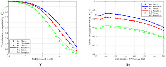
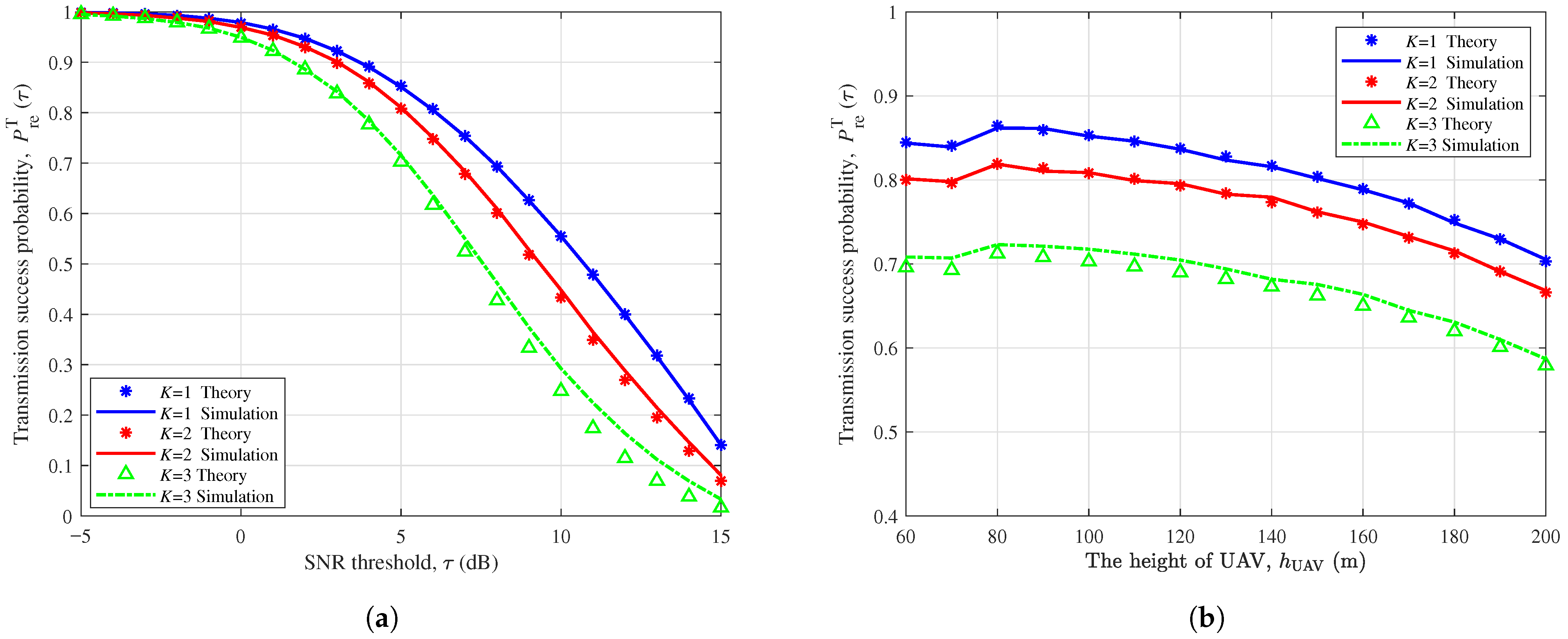
In the figures, the simulation results are obtained by averaging over 50,000 Monte Carlo simulation realizations through MATLAB R2024a, while the theoretical results are derived using the Mathematica 14.0 platform. Markers represent the theoretical results via our derived expressions, and solid lines represent the simulation results. Figure 2 shows that the transmission success probability of regular data under the TDMA scheme varies with (a) predefined SNR threshold and (b) the height of the UAV, respectively. The theoretical results match well with the simulation results, validating our analytical analysis. In Figure 2a, we can observe that as the SNR threshold increases, the transmission success probability decreases monotonically. This is because a higher threshold requirement poses a stricter signal strength level, reducing the proportion of transmission instances that can satisfy the condition. Moreover, the rate of decrease is faster when K = 3 than when K = 1, since when K = 3 the SNR requirement must be simultaneously satisfied by the first, second, and third MDs transmitting to the serving RB, thereby significantly increasing the likelihood of transmission failure in marine data acquisition. In Figure 2b, it is observed that as the UAV height increases from 60 m to 200 m, the transmission success probability initially exhibits a slight rise and then gradually decreases. This trend occurs because, when the UAV height increases from 60 m to 80 m, following the two-ray path loss model, the LoS and refracted signal components between the RB and the serving UAV constructively combine, enhancing the received signal strength. However, as the UAV ascends further, the link distance between the RB and the UAV becomes longer, resulting in increased path loss and a subsequent decline in transmission success probability. In addition, in Figure 2a,b, the discrepancy between the theoretical and simulation results appears when K = 3. This is because, for K = 3, the theoretical analysis involves the joint transmission success probability of three MDs, which aggregates individual link-level performance metrics. Although the discrepancy for each MD is relatively small, these errors accumulate when their joint performance is evaluated, leading to a more noticeable deviation compared to the single MD case.

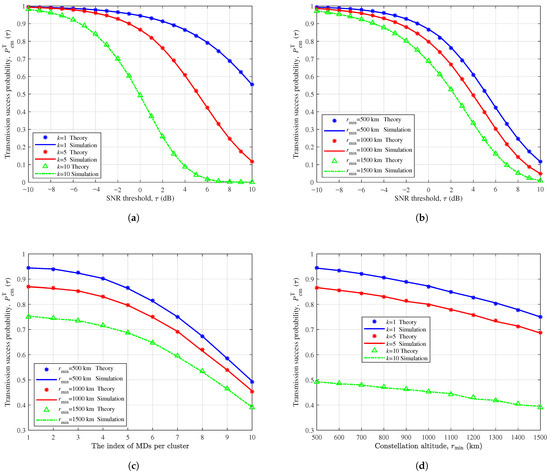
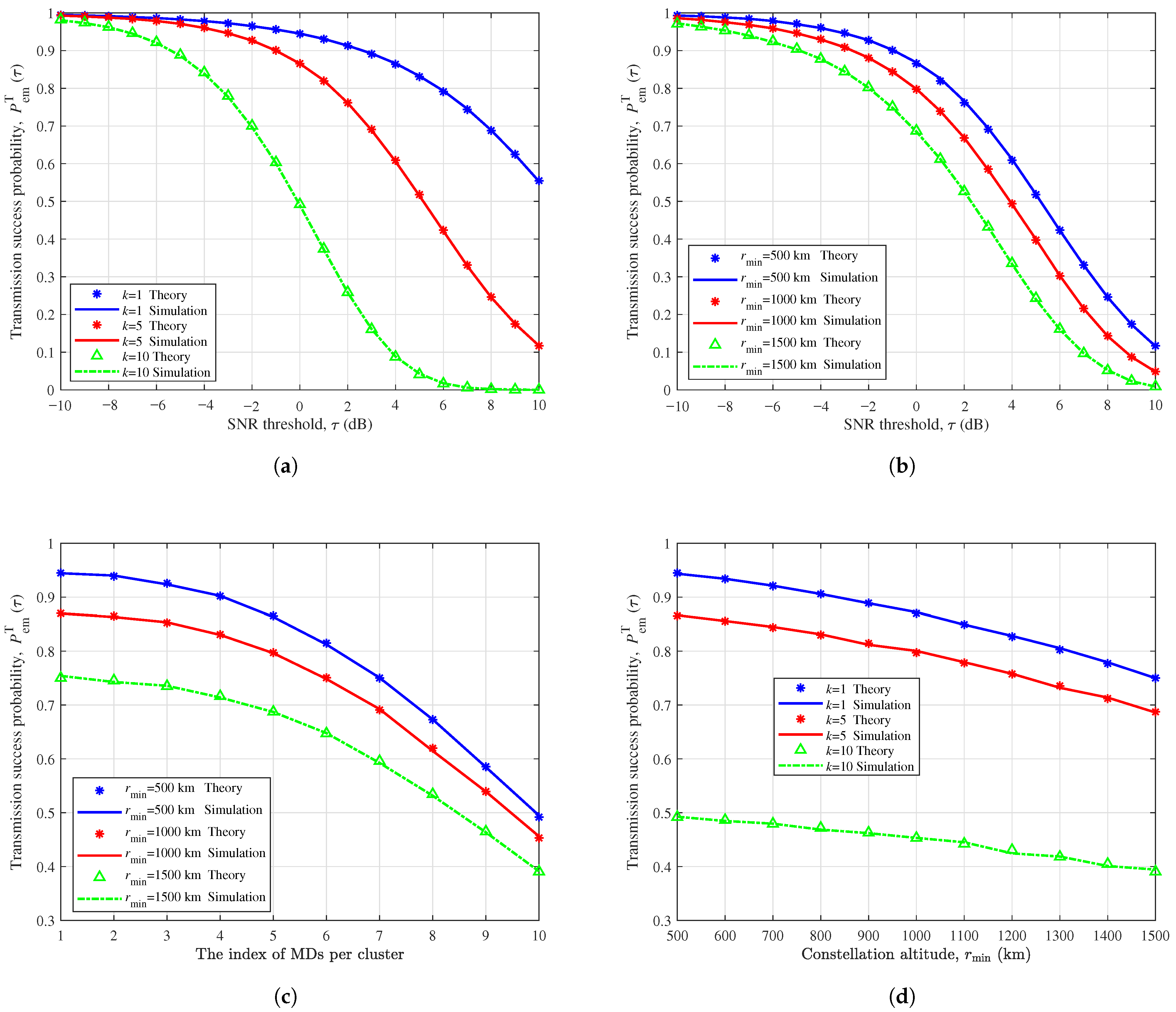
Figure 3 validates the theoretical analysis of the transmission success probability of emergency data under TDMA scheme. Specifically, Figure 3a,b illustrate the variation of transmission success probability with respect to the predefined SNR threshold under different MD indices and constellation altitudes. As the SNR threshold increases, the transmission success probability exhibits a monotonically decreasing trend, since a higher SNR requirement reduces the proportion of transmission instances that satisfy the threshold in both the marine and space links. Figure 3c depicts the transmission success probability as a function of the MD index within each cluster. A clear downward trend is observed as the MD index increases. This is attributed to the fact that a larger MD index corresponds to a longer distance between the $k^{\mathrm{th}}$ MD and the serving RB, resulting in higher path loss in the marine link and thus a lower transmission success probability. Figure 3d presents the influence of constellation altitude on the transmission success probability. A higher constellation altitude leads to degraded performance because the increased distance between the RB and the serving satellite introduces higher path loss in the space link. Moreover, under a constellation altitude of 1000 km, when k increases from one to five, the transmission success probability decreases by approximately 7.29%. However, when k increases from five to ten, it drops sharply by nearly 34.41%. This indicates that when the MD index is small, the transmission performance is mainly limited by the satellite altitude, which predominantly affects the space link. In contrast, as the MD index becomes larger, the marine link becomes the dominant bottleneck, leading to a pronounced degradation in transmission success probability of emergency data.

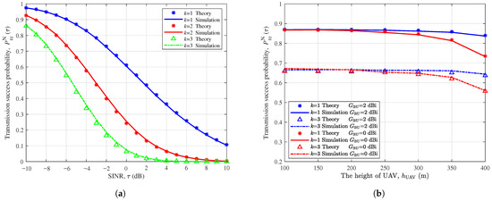
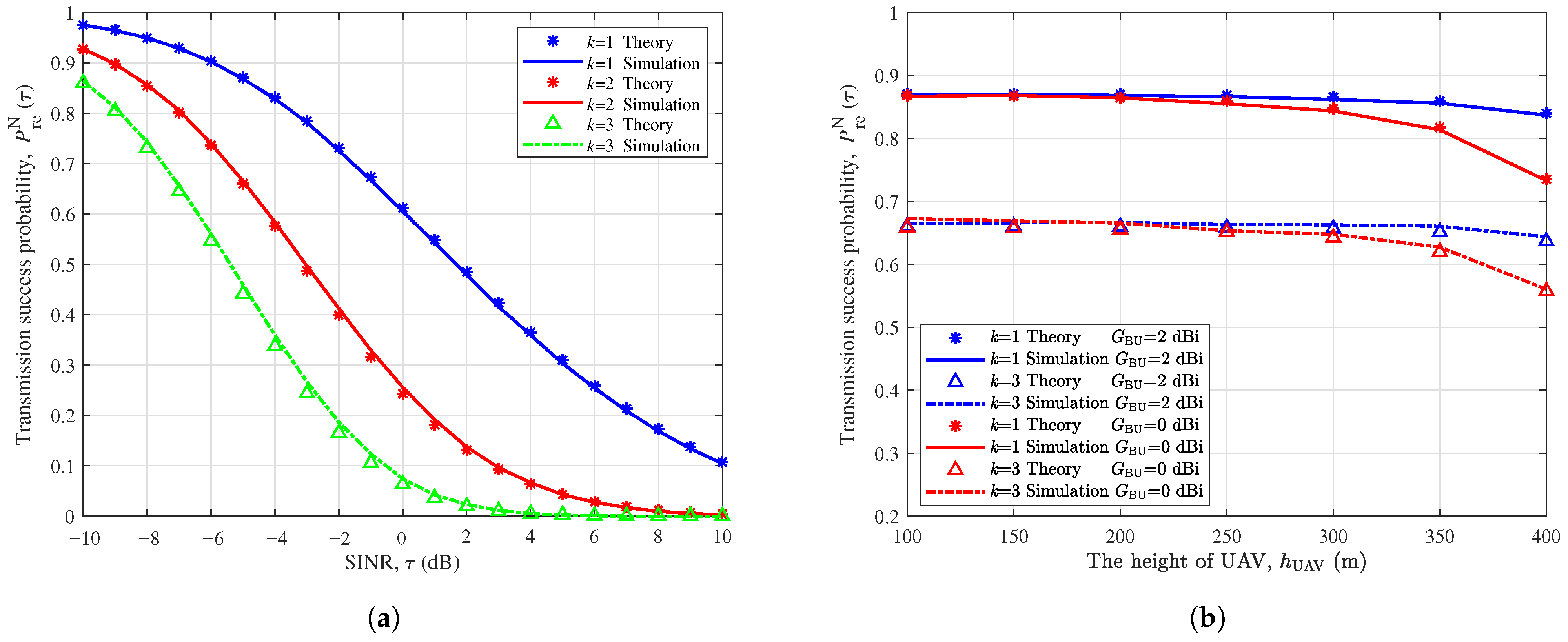
Figure 4 validates the theoretical analysis of the transmission success probability of regular data under the NOMA scheme. Figure 4a shows its variation with the predefined SINR threshold. It can be observed that the transmission success probability under the NOMA scheme is considerably lower than that under the TDMA scheme. This performance degradation primarily results from the interference introduced by MDs within the same cluster sharing the marine channel via the NOMA scheme, which reduces the effective received signal strength. Figure 4b illustrates the impact of UAV altitude on the transmission success probability when $G_{\mathrm{BU}}$ is set to 2 dB and 0 dB, respectively. The curves remain nearly unchanged as the UAV height increases from 60 m to 200 m, indicating that, under the given parameter settings, the transmission performance is predominantly limited by the interference in the marine link, while the air link has a comparatively minor effect.

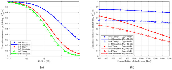
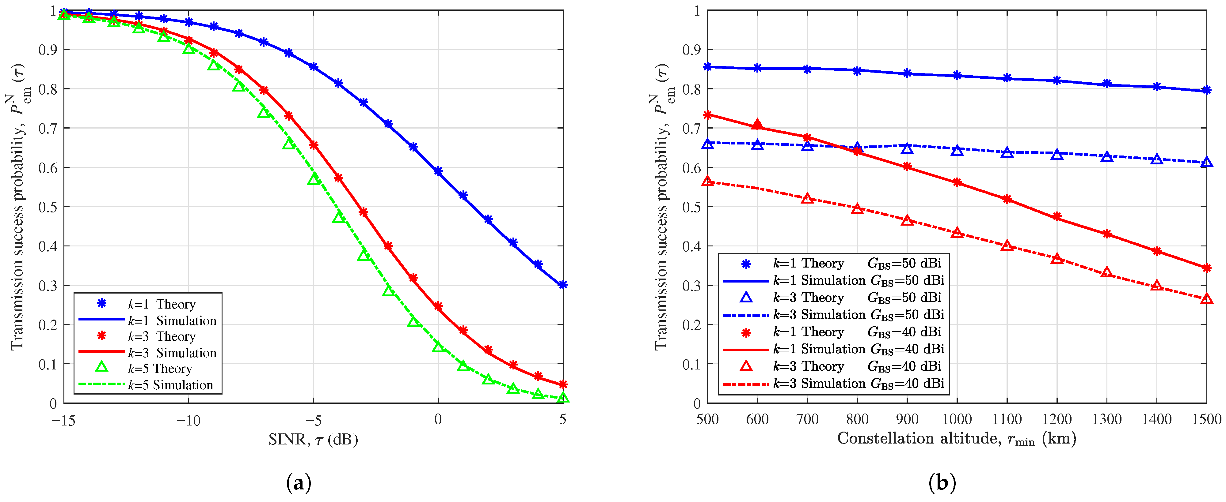
Figure 5 illustrates the transmission success probability of emergency data under the NOMA scheme with varying network parameters. It again confirms the accuracy of the theoretical analysis. Specifically, Figure 5a depicts the impact of the predefined SINR threshold. It can be observed that, compared with Figure 3a, the transmission success probability under NOMA is significantly lower than that under the TDMA scheme. For instance, when the $\tau =-6$ dB and k = 5, the transmission success probability under TDMA reaches 0.922, whereas that under NOMA decreases to 0.656. This degradation is mainly attributed to the interference introduced by MDs sharing the same marine channel, which reduces the effective received signal power. Correspondingly, Figure 5b shows the effect of constellation altitude on the transmission success probability when $G_{\mathrm{BS}}$ is set to 50 dBi and 40 dBi, respectively. The results imply that achieving more reliable transmission performance requires a higher antenna gain.

Figure 6 illustrates the end-to-end delay of emergency data under the TDMA scheme with respect to (a) constellation altitude, (b) the MD index within each cluster, and (c) the number of MDs per cluster. In Figure 6a, the end-to-end delay is evaluated when the time slot duration $\Delta T$ is set to 10⁻⁶ s and 10⁻³ s, respectively. The theoretical results align well with the simulations, verifying the accuracy of the analytical derivation. When $\Delta T={10}^{-3}\mathrm{s}$, the end-to-end delay remains nearly constant across different constellation altitudes, as the queuing delay dominates the end-to-end delay. In this case, MDs spend considerable time waiting in queues, indicating that although the TDMA scheme eliminates interference during signal transmissions, it inevitably introduces additional queuing delays to marine data acquisition. In contrast, when $\Delta T={10}^{-6}\mathrm{s}$, the end-to-end delay increases slightly with constellation altitude, suggesting that both queuing and transmission delays jointly affect the end-to-end delay under the given parameter settings. Furthermore, when k = 10, the end-to-end delay is significantly higher than that for k = 2 and k = 5, primarily because the longer distance in the marine link has a pronounced impact on the end-to-end delay due to the harsh maritime environmental factors.

In Figure 6b, the end-to-end delay initially decreases from the first to the second MD owing to the nonlinear signal attenuation characterized by the two-ray path loss model. As the MD index further increases, the delay begins to rise. This trend occurs because a larger MD index corresponds to a longer $R_{\mathrm{MB},k}$, where the path loss becomes the dominant factor affecting transmission performance, resulting in a reduced data rate in the marine link and consequently an increased end-to-end delay. Figure 6c illustrates the variation of end-to-end delay with the number of MDs per cluster when k is set to 2, 5, and the last MD, respectively. It can be observed that when k = 2 and 5, the end-to-end delay decreases gradually. This occurs because, in these case, the path loss in the marine link becomes the dominant factor over queuing delay. As $N_{\mathrm{M}}$ increases, the fifth MD is positioned closer to the serving RB, resulting in reduced path loss and, consequently, lower end-to-end delay. Therefore, under the TDMA scheme, the node closest to the serving RB does not necessarily achieve the best delay performance. In contrast, when $k=N_{\mathrm{M}}$, the end-to-end delay increases gradually. This is because, as the number of MDs per cluster increases, more time slots are allocated within the channel, leading to a longer queuing delay. Meanwhile, the combined effect of path loss and queuing delay leads to a moderate and steady increase in the overall delay.

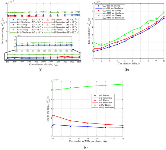
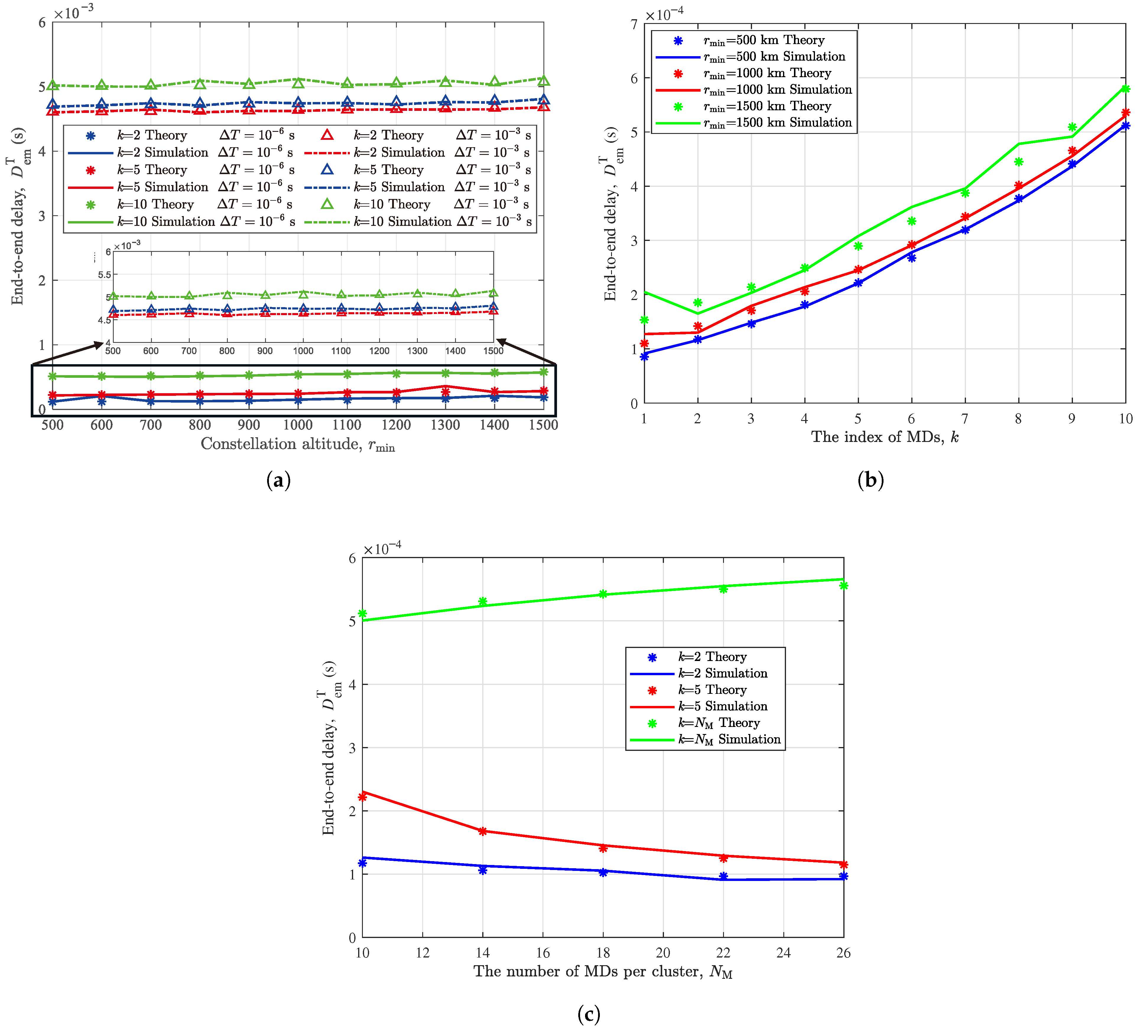
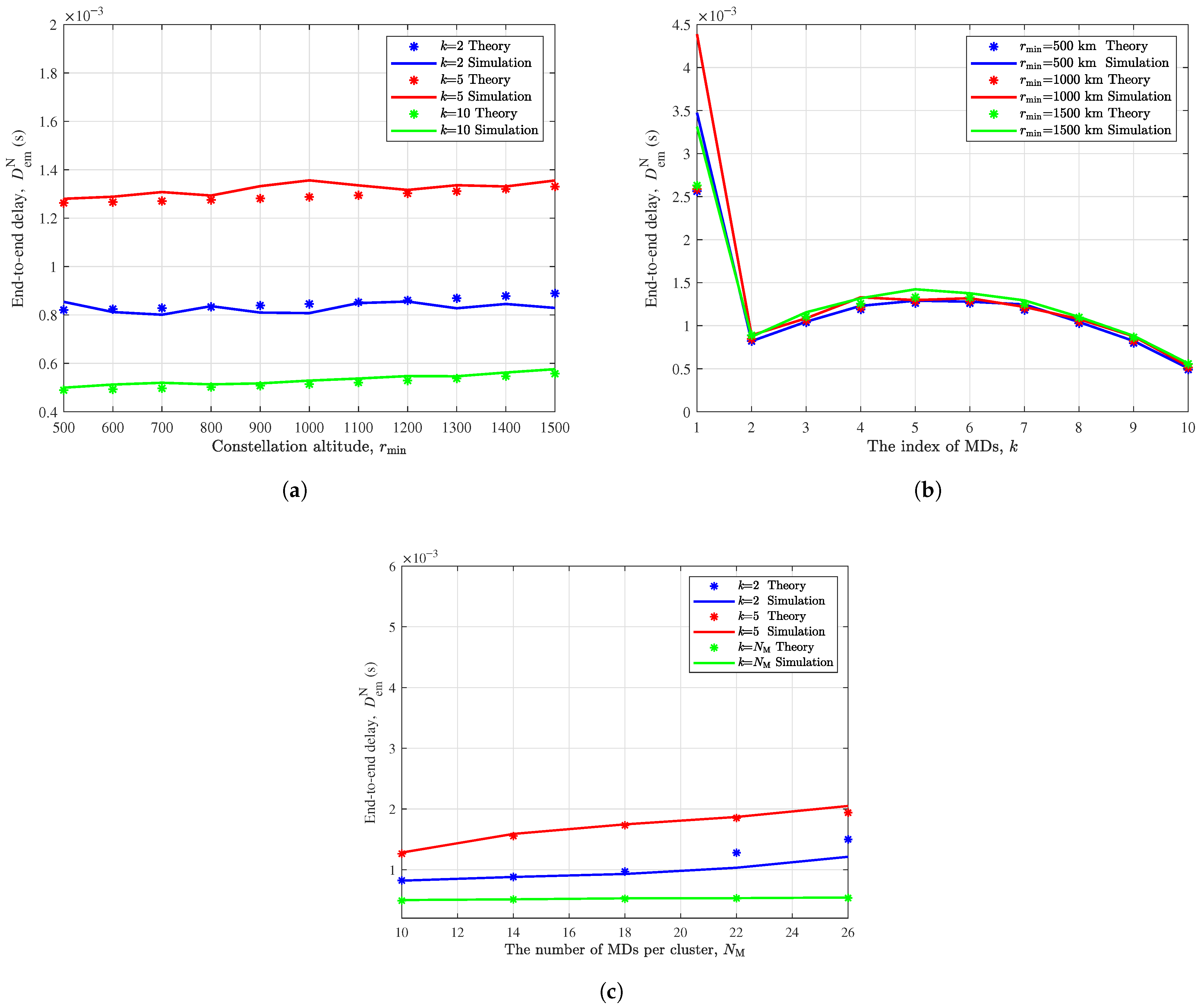
The validation of the end-to-end delay of emergency data under the NOMA scheme is presented in Figure 7. In Figure 7a, the end-to-end delay is shown as a function of the constellation altitude for k = 2, 5, and 10. Theoretical results exhibit close agreement with simulations, confirming the accuracy of the analytical derivations. As the constellation altitude increases, the end-to-end delay remains nearly constant. This is attributed to the dominant influence of interference within the shared marine channel, which mitigates the effect of the space link on delay performance. Under the same conditions ($r_{\min }=1000\mathrm{km}$, and k = 5), the end-to-end delay under the NOMA scheme is 0.00129 s, compared with 0.00025 s under the TDMA scheme with $\Delta T={10}^{-6}$ s, highlighting the significant impact of interference on the transmission performance of the LSU-MIoT network. Therefore, for scenarios with short data packets (requiring a short duration per time slot) and a small number of MDs per cluster, the TDMA scheme is preferable, as it ensures stable transmission reliability and yields a lower end-to-end delay.

Figure 7b illustrates the variation of end-to-end delay of emergency data with the MD index under the NOMA scheme. Similar to Figure 6b, the delay initially decreases from the first to the second MD due to the nonlinear attenuation caused by the two-ray path loss model. As the MD index increases from two to five, the delay gradually rises. This occurs because the number of interfering MDs decreases with increasing index, as interference primarily originates from MDs located farther from the $k^{\mathrm{th}}$ MD in each cluster. Consequently, the reduction in interference power contributes to the increase of distance from the MD to the RB, leading to an increase in delay. Beyond this range, as the index continues to grow, the delay gradually declines again, dominated due to the SINR improvement. Figure 7c presents the impact of the number of MDs per cluster on the end-to-end delay. In contrast to Figure 6c, the delay when k = 2 is greater than that when $k=N_{\mathrm{M}}$. This is because when k = 2, there are $N_{\mathrm{M}}-2$ interfering MDs within the cluster, while no interference occurs when $k=N_{\mathrm{M}}$, resulting in stronger received signal power and thus a smaller delay. Therefore, in cases where emergency data is generated from MDs positioned at the rear of a cluster, switching to the NOMA scheme is recommended, as it mitigates interference and removes queuing delay.

5. Conclusions

In this article, we have considered an LSU-MIoT network and established a theoretical framework to analytically evaluate network performance in supporting marine data acquisition. Specifically, RBs and MDs are modeled as a Matérn cluster process on the sea surface, UAVs as an HPPP at a fixed height over the sea surface, and LEO satellites as an SPPP on a sphere surface. Signal transmissions are initiated from MDs to the serving RB over the marine link and are subsequently relayed to the UAV over the air link or to the LEO satellite over the space link, subject to Nakagami-m, Rician, and SR fading, respectively, with two-ray path loss applied to sea and air links. This framework aims to capture key performance metrics, including the transmission success probability and the end-to-end delay of regular and emergency data under the TDMA and NOMA schemes, leveraging the tool of stochastic geometry. Extensive results validate the theoretical analysis and reveal the impact of network parameters on the performance of the LSU-MIoT network. It can be concluded that for scenarios with short data packets and a small number of MDs per cluster, the TDMA scheme is preferable, whereas switching to the NOMA scheme is recommended when emergency data are generated by MDs located at the edge of a cluster in the LSU-MIoT network. The framework is expected to provide theoretical guidance for the design of next-generation maritime communication infrastructures to enhance the efficiency and reliability of marine data acquisition.

For the potential follow-up research, several directions can be further investigated. On the one hand, the analytical framework may be further extended to incorporate inter-cluster interference to characterize the performance in the scenario where multiple clusters share the same marine channel. On the other hand, additional performance metrics relevant to practical maritime communications, such as marine link availability, can be investigated while accounting for ocean-specific environmental factors. Then, advanced multiple access schemes, such as rate-splitting multiple access (RSMA) [30], can also be can be incorporated to investigate achievable performance boundaries of the LSU-MIoT network under different access schemes.

References

- Jung, S.; Jeong, S.; Kang, J.; Kang, J. Marine IoT Systems with Space–Air–Sea Integrated Networks: Hybrid LEO and UAV Edge Computing. IEEE Internet Things J. 2023, 10, 20498–20510. [Google Scholar] [CrossRef] [Scilit]
- Qian, L.P.; Zhang, H.; Wang, Q.; Wu, Y.; Lin, B. Joint Multi-Domain Resource Allocation and Trajectory Optimization in UAV-Assisted Maritime IoT Networks. IEEE Internet Things J. 2023, 10, 539–552. [Google Scholar] [CrossRef] [Scilit]
- Hu, X.; Wang, Y.; Lin, B.; Wei, H. Stochastic Geometry Based Modeling and Performance Analysis of Buoy-Assisted Offshore Internet of Things. In Proceedings of the 2023 IEEE International Conferences on Internet of Things (iThings) and IEEE Green Computing & Communications (GreenCom) and IEEE Cyber, Physical & Social Computing (CPSCom) and IEEE Smart Data (SmartData) and IEEE Congress on Cybermatics (Cybermatics), Danzhou, China, 17–21 December 2023; Available online: https://ieeexplore.ieee.org/document/10501861 (accessed on 1 May 2024).
- Xia, T.; Wang, M.M.; Zhang, J.; Wang, L. Maritime Internet of Things: Challenges and Solutions. IEEE Wirel. Commun. 2020, 27, 188–196. [Google Scholar] [CrossRef] [Scilit]
- Hu, H.; Yu, Q.; Zhang, R.; Ye, Y.; Jiang, F.; Jiang, J.; Niyato, D. Minimizing Energy Consumption in UAV-Assisted Maritime Wireless Powered Networks with Constrained Age of Information. IEEE Trans. Cogn. Commun. Netw. 2025; early access. Available online: https://ieeexplore.ieee.org/document/11202256 (accessed on 13 October 2025).
- Guan, S.; Wang, J.; Jiang, C.; Duan, R.; Ren, Y.; Quek, T.Q.S. MagicNet: The Maritime Giant Cellular Network. IEEE Commun. Mag. 2021, 59, 117–123. [Google Scholar] [CrossRef] [Scilit]
- Lu, X.; Salehi, M.; Haenggi, M.; Hossain, E.; Jiang, H. Stochastic Geometry Analysis of Spatial-Temporal Performance in Wireless Networks: A Tutorial. IEEE Commun. Surv. Tutor. 2021, 23, 2753–2801. [Google Scholar] [CrossRef] [Scilit]
- Xu, J.; Kishk, M.A.; Alouini, M.S. Space-Air-Ground-Sea Integrated Networks: Modeling and Coverage Analysis. IEEE Trans. Wirel. Commun. 2023, 22, 6298–6313. [Google Scholar] [CrossRef] [Scilit]
- Xiong, K.; Chen, X.; Ying, M. On the Performance of Integrated Satellite–Terrestrial Maritime Communications. IEEE Internet Things J. 2025, 12, 36183–36196. [Google Scholar] [CrossRef] [Scilit]
- Gao, Q.; Su, L.; Fu, J.; Lin, Y. Successful Transmission Probability Analysis of the Satellite-Maritime Uplink: A Stochastic Geometry Based Approach. Mobile Netw. Appl. 2025, 30, 115–126. [Google Scholar] [CrossRef] [Scilit]
- Li, Z.; Shang, B. Fundamentals of Satellite-Maritime Communications: Downlink and Uplink Analysis. IEEE Trans. Commun. 2025, 73, 2191–2206. [Google Scholar] [CrossRef] [Scilit]
- Hu, X.; Lin, B.; Lu, X.; Wang, P.; Cheng, N.; Yin, Z.; Zhuang, W. Performance Analysis of End-to-End LEO Satellite-Aided Shore-to-Ship Communications: A Stochastic Geometry Approach. IEEE Trans. Wirel. Commun. 2024, 23, 11753–11769. [Google Scholar] [CrossRef] [Scilit]
- Xu, J.; Kishk, M.A.; Alouini, M.S. Coverage Enhancement of Underwater Internet of Things Using Multilevel Acoustic Communication Networks. IEEE Internet Things J. 2022, 9, 25373–25385. [Google Scholar] [CrossRef] [Scilit]
- Xu, J.; Kishk, M.A.; Zhang, Q.; Alouini, M.S. Three-Hop Underwater Wireless Communications: A Novel Relay Deployment Technique. IEEE Internet Things J. 2023, 10, 13354–13369. [Google Scholar] [CrossRef] [Scilit]
- Li, S.; Zhang, J.; Li, J.; Xie, Y.; Pan, G. Physical-Layer Security for Multiantenna Satellite-UWOC Systems in the Presence of Spatially Random Locations. IEEE Internet Things J. 2024, 11, 27480–27493. [Google Scholar] [CrossRef] [Scilit]
- Senadhira, N.; Durrani, S.; Guo, J.; Yang, N.; Zhou, X. Design and Performance Analysis of UAV-Assisted Maritime-LEO Satellite Communication Networks. IEEE Open J. Commun. Soc. 2025, 6, 4667–4688. [Google Scholar] [CrossRef] [Scilit]
- Wang, Q.; Dai, H.N.; Wang, Q.; Shukla, M.K.; Zhang, W.; Soares, C.G. On Connectivity of UAV-Assisted Data Acquisition for Underwater Internet of Things. IEEE Internet Things J. 2020, 7, 5371–5385. [Google Scholar] [CrossRef] [Scilit]
- Park, J.; Choi, J.; Lee, N. A Tractable Approach to Coverage Analysis in Downlink Satellite Networks. IEEE Trans. Wirel. Commun. 2023, 22, 793–807. [Google Scholar] [CrossRef] [Scilit]
- Shi, H.; Deng, N.; Li, B.; Wei, H.; Lu, W.; Zhao, N. Modeling and analysis of satellite-terrestrial covert communications. Sci. China Inf. Sci. 2025, 68, 190306. [Google Scholar] [CrossRef] [Scilit]
- Tabassum, H.; Hossain, E.; Hossain, J. Modeling and Analysis of Uplink Non-Orthogonal Multiple Access in Large-Scale Cellular Networks Using Poisson Cluster Processes. IEEE Trans. Commun. 2017, 65, 3555–3570. [Google Scholar] [CrossRef]
- Qin, Z.; Liu, Y.; Li, G.Y.; McCann, J.A. Performance Analysis of Clustered LoRa Networks. IEEE Trans. Veh. Technol. 2019, 68, 7616–7629. [Google Scholar] [CrossRef] [Scilit]
- Zöchmann, E.; Guan, K.; Rupp, M. Two-ray models in mmWave communications. In Proceedings of the 2017 IEEE 18th International Workshop on Signal Processing Advances in Wireless Communications (SPAWC), Sapporo, Japan, 3–6 July 2017; Available online: https://ieeexplore.ieee.org/document/8227681 (accessed on 21 December 2017).
- Wang, J.; Zhou, H.; Li, Y.; Sun, Q.; Wu, Y.; Jin, S.; Quek, T.Q.S.; Xu, C. Wireless Channel Models for Maritime Communications. IEEE Access 2018, 6, 68070–68088. [Google Scholar] [CrossRef] [Scilit]
- He, Y.; Li, Z.; Chen, Y. Tractable Modeling and Performance Analysis of Low-Earth Orbit Satellite Constellations. IEEE Internet Things J. 2024, 11, 28297–28306. [Google Scholar] [CrossRef] [Scilit]
- Sun, Y.; Ding, Z. A Fine Grained Stochastic Geometry-Based Analysis on LEO Satellite Communication Systems. IEEE Netw. Lett. 2023, 5, 237–240. [Google Scholar] [CrossRef] [Scilit]
- Li, X.; Wang, Q.; Peng, H.; Zhang, H.; Do, D.T.; Rabie, K.M.; Kharel, R.; Cavalcante, C.C. A Unified Framework for HS-UAV NOMA Networks: Performance Analysis and Location Optimization. IEEE Access 2020, 8, 13329–13340. [Google Scholar] [CrossRef] [Scilit]
- Lin, X.; Zhang, H.; Pan, G.; Wang, S.; An, J. LEO Relay-Aided GEO Satellite-Terrestrial Transmissions. IEEE Trans. Veh. Technol. 2023, 72, 16899–16904. [Google Scholar] [CrossRef] [Scilit]
- Zheng, J.; Wang, Z.; Jamalipour, A. An Aerial and Ground Base Station Cooperation Strategy for UAV and Cellular Integrated Networks. IEEE Internet Things J. 2024, 11, 10411–10424. [Google Scholar] [CrossRef] [Scilit]
- Paris, J.F. Statistical Characterization of κ−μ Shadowed Fading. IEEE Trans. Veh. Technol. 2014, 63, 518–526. [Google Scholar] [CrossRef] [Scilit]
- Min, L.; Li, J.; He, Y.; Wang, W. Secure Rate-Splitting Multiple Access for Maritime Cognitive Radio Network: Power Allocation and UAV’s Location Optimization. J. Mar. Sci. Eng. 2023, 11, 1012. [Google Scholar] [CrossRef] [Scilit]
Disclaimer/Publisher’s Note: The statements, opinions and data contained in all publications are solely those of the individual author(s) and contributor(s) and not of MDPI and/or the editor(s). MDPI and/or the editor(s) disclaim responsibility for any injury to people or property resulting from any ideas, methods, instructions or products referred to in the content. |
© 2026 by the authors. Licensee MDPI, Basel, Switzerland. This article is an open access article distributed under the terms and conditions of the Creative Commons Attribution (CC BY) license.