Optimizing Trajectories for Rechargeable Agricultural Robots in Greenhouse Climatic Sensing Using Deep Reinforcement Learning with Proximal Policy Optimization Algorithm ^†

Abstract

The experimentation of agricultural robots has been increasing in recent years, both in greenhouses and open fields. While agricultural robots are inherently useful for automating various farming tasks, their presence can also be leveraged to collect measurements along their paths. This approach enables the creation of a complete and detailed picture of the climate conditions inside a greenhouse, reducing the need to distribute a large number of physical devices among the crops. In this regard, choosing the best visiting sequence of the Points of Interest (PoIs) regarding where to perform the measurements deserves particular attention. This trajectory planning has to carefully combine the amount and significance of the collected data with the energy requirements of the robot. In this paper, we propose a method based on Deep Reinforcement Learning enriched with a Proximal Policy Optimization (PPO) algorithm for determining the best trajectory an agricultural robot must follow to balance the number of measurements and autonomy adequately. The proposed approach has been applied to a real-world case study regarding a greenhouse in Verona (Italy) and compared with other existing state-of-the-art approaches.

1. Introduction

Greenhouses are typically controlled environments, but considering uniform climate conditions inside them is unrealistic and sometimes harmful for plants health and growth [1]. This fact was originally discussed in the late 1990s, with a focus on humidity and transpiration [2]. Similarly, in [3], the authors revealed the presence of different micro-climates around plants. Starting from these works, other studies like [4,5,6,7,8,9] confirmed that relying on spatially accurate information about the micro-climate inside a greenhouse is an extremely important but challenging task. In this domain, technology provides the possibility of measuring and controlling climate variation within the greenhouse. For instance, today, there is a wide range of sensors to monitor different parameters, including air temperature and humidity [10], soil moisture [11], soil irrigation volume, light intensity, and carbon dioxide concentration [12]. However, a significant level of spatial accuracy typically comes with costs regarding the number of sensors to be installed inside the greenhouse. In addition, physical and technological installation constraints must be addressed, which include power supplies, battery and charging of sensor networks, periodic calibration and synchronization, sensor maintenance, avoiding risk of sensor damage in high-temperature and humidity environments, and the impossibility of installing a physical device at each point of interest [13].

The so-called virtual sensors, also referred to as soft sensors, represent a viable and cost-effective solution to these issues. A virtual sensor is essentially a software model that surrogates a hardware device to provide real-time information at specific points of interest [14]. In [15], a Recurrent Neural Network (RNN)-based technique is presented for constructing virtual sensors trained with data previously collected through temporary sensors inside the greenhouse. In this case, introducing several contextual dimensions of analysis allows for an effective model to predict climatic conditions in several greenhouse locations. Figure 1 illustrates an example of this approach, where seven temporary sensors have been placed in specific points of interest (denoted as $po{i}_i$) of the greenhouse (e.g., close to particular plant rows) together with a permanent sensor $cs$, positioned at the center. Each temporary sensor is used for a limited period to collect enough data to understand the relation between the temperature at that point in different time slots, periods of the year, weather conditions, and the measurements provided by $cs$. The corresponding virtual sensors $v{s}_i$ can be created for each point of interest as a trained RNN model to replace physical sensors effectively [16].

A more efficient solution is the substitution of the temporary sensors with an agricultural robot that follows a predefined trajectory in the greenhouse to perform its farming tasks [17]. As shown in Figure 2, the robot stops at each PoI during every complete round and regularly takes a measurement in that location.

Despite the merits of such solutions, as highlighted in [18], the strategy of periodically stopping in all PoIs is not always the best one. In certain periods, some PoIs could be more interesting than others; thus, in those periods, it could be more preferable to stop more frequently in those PoIs and only occasionally in others. Moreover, the set of interesting PoIs can change over time based on the context or situation of interest in a dynamic way that can be hardly addressed by traditional operational research approaches. Considering all of these, in [18], we start to investigate the problem of identifying the best stopping pattern for the robot based on the contextual importance of each PoI in the current measurement process. For instance, with reference to the configuration shown in Figure 2, the approach of [18] might determine that in a specific contextual situation, $po{i}_4$ and $po{i}_6$ are not interesting and the robot can pass through them without stopping and taking measurements. This strategy leads to reducing the time needed to complete the trajectory and increasing the sampling rate of the visited PoIs.

In this paper, we take a step forward in the definition of the best measuring stopping pattern by carefully combining the amount and significance of the collected data with the energy aspects of the agricultural robot. In particular, we introduce a more complex model of the environment, which considers the energy consumption associated with each path and that some PoIs not only represent a source of data but also are charging stations. Moreover, different alternative paths may exist from one PoI to another, with different energy costs and benefits in terms of monitoring and recharging opportunities. In particular, the identification of the best stopping pattern is obtained as a combination of a deep reinforcement learning approach and a proximal policy optimization algorithm, which are used together to balance the number and quality of measurements adequately with the robot’s autonomy. The reason behind this selection is that in this study, we are dealing with a complex scenario of trajectory optimization for a rechargeable robot operating in a greenhouse environment. DRL provides a data-driven approach to learn optimal decision-making policies in such dynamic and uncertain environments. Among available DRL methods, we adopt the PPO algorithm, which offers a favorable balance between sample efficiency, exploration, and training stability. PPO’s clipped surrogate objective prevents destabilizing policy updates, making it especially suited to robotic applications involving continuous learning. Through the PPO framework, the robot learns to adaptively schedule its movements, decide when to recharge, and select trajectories that maximize cumulative measurement reward without exceeding energy constraints.

Figure 3, illustrates an example of the mentioned enriched environment where some paths have been added. With respect to Figure 2, the arrows have been removed to denote the possibility to travel in both directions, and charging stations have been positioned at some PoIs.

For example, from $po{i}_5$, it is possible to directly reach the charging stations in $po{i}_7$ and $po{i}_3$, while from the charging station in $po{i}_7$, it is possible to directly reach $po{i}_2$ without visiting $po{i}_1$ or going back to $po{i}_6$.

To the best of our knowledge, this paper is the first attempt to combine background knowledge about the robot (autonomy and velocity) and the environment (possible paths and position of charging stations) with historical properties on collected data, thus creating a mixed model-driven and data-driven approach. In the following subsection, we review related work in this domain, highlighting the differences and limitations with respect to the proposed approach.

Related Work

As mentioned, wireless sensor networks (WSNs) are a useful framework that allows farmers and researchers to monitor real-time data precisely. This possibility could be beneficial for farmers to manage the required resources of their fields and improve their crop yields [19]. In [20], a dense WSN was used for greenhouse climate control. Simulations on monitoring and controlling greenhouse climate using WSNs were conducted in [14]. Building on this, in [21], the authors studied the application of WSNs for controlling greenhouse parameters in precision agriculture. In 2015, a study conducted in a Greek greenhouse indicated the capabilities of WSNs in achieving spatially distributed climate control. In this regard, [22] proposed a hierarchical WSN system for greenhouse monitoring, combining Internet technology and intelligent object communication models.

As highlighted in the introduction, despite the undeniable success of WSNs in greenhouses, they suffer from various shortcomings in different aspects, which leads to increasing interest in virtual sensors. As indicated in [23], the application of virtual sensors in greenhouses is limited but includes many different attempts [24,25,26,27].

In general, virtual sensing approaches can be divided into two main categories: model-based and data-driven methods [28]. Model-based virtual sensors exploit system knowledge described through equations [29], while data-driven virtual sensors rely on historical measurements, which serve as input for statistical or machine learning methods [30,31]. A typical example of a model-driven approach is represented by the use of computational fluid dynamics (CFDs) rules that model fluid flows inside the greenhouses [32,33,34]. Studies in this area have concentrated on CFD simulations for analyzing experimental data [35], forecasting temperature distribution [36], creating dynamic models for greenhouses [37], and investigating thermal balance in greenhouse air conditioning systems [38]. Recent advancements include the integration of machine learning with CFD to improve accuracy and efficiency in fluid flow simulations [39] and the development of virtual sensor systems for real-time monitoring of greenhouse parameters like temperature, humidity, and CO₂ [40]. However, this approach remains challenging due to its complexity, high computational requirements, and sensitivity to disturbances in greenhouse environments [34].

Unlike the model-based approach, data-driven virtual sensors estimate physical conditions using available data, statistical methods, and state-of-the-art machine learning techniques. For instance, the relationship between temporary and permanent sensors, considering both time and spatial context, is captured by linear regression in [41] and by a trained recurrent neural network (RNN) in [15]. The method presented in [42] uses reinforcement learning (RL) to manage sensor states. In this method, the agent learns from LSTM-based predictions to determine the best times to activate or deactivate sensors, aiming to save energy while maintaining accuracy.

2. Materials and Methods

This section summarizes some background notions, formalizes the problem under investigation, and provides details about the proposed solution and implementation details.

2.1. Background

RL is a machine learning technique in which an agent interacts with its environment by making observations, taking actions based on those observations, and receiving rewards that reflect the resulting state changes. The sequence of actions chosen by the agent represents the so-called policy, and the final goal of the agent is to find the best policy, namely the one that maximizes the cumulative reward obtained through the sequence of actions taken in various states. Indeed, while the reward associated with each action a performed in a given state s represents the goodness of a in the short term, the cumulative reward represents the goodness of the entire strategy in the long term. In this case, the learning process is based on the continuous interaction of the agent with the environment.

Reinforcement learning (RL) has seen remarkable progress in recent years, especially with the advent of deep reinforcement learning (DRL), in which neural networks are used to approximate the functions needed to perform the training and identify the best policy. Several variants of DRL have been proposed in the literature, differing in how they model agent–environment interactions and compute the optimal policy efficiently. In this paper, we use a method known as the Proximal Policy Optimization (PPO) algorithm [43].

PPO works by iteratively improving the policy through a trial-and-error approach through which it trains a stochastic policy ${\pi }_{\theta }$, allowing the agent to explore different actions and observe their outcomes. During each training cycle, the agent collects fresh trajectories (i.e., sequences of states, actions, and rewards) using the current version of the policy. These recent trajectories are then used to update the policy in a way that maximizes the expected reward. As the number of interactions increases, the agent’s actions become progressively less random and more accurate.

PPO is a first-order optimization method for RL that balances simplicity, stability, and performance. Unlike standard policy gradient methods, which suffer from high variance and instability, like the Deep Q-Learning (DQL) method [18] or Trust Region Policy Optimization (TRPO), which requires complex constrained optimization, PPO avoids large, destabilizing policy updates by introducing a clipping mechanism in the objective function. In particular, a clipping region is used to restrict the difference between the new and old policy to a small, controlled range. This proximal update ensures that learning remains stable and does not diverge, which is especially beneficial in complex environments or in the presence of limited training data.

PPO is implemented with an actor–critic architecture. The actor network (or policy network) selects actions to take, while the critic network (or value network) estimates state values to compute the goodness of the choices taken. Figure 4 shows the architecture of the PPO algorithm using an actor–critic approach. As illustrated in the figure, the system operates in a continuous loop with the aim of refining both the actor’s decisions and the critic’s evaluations. It includes the following main components:

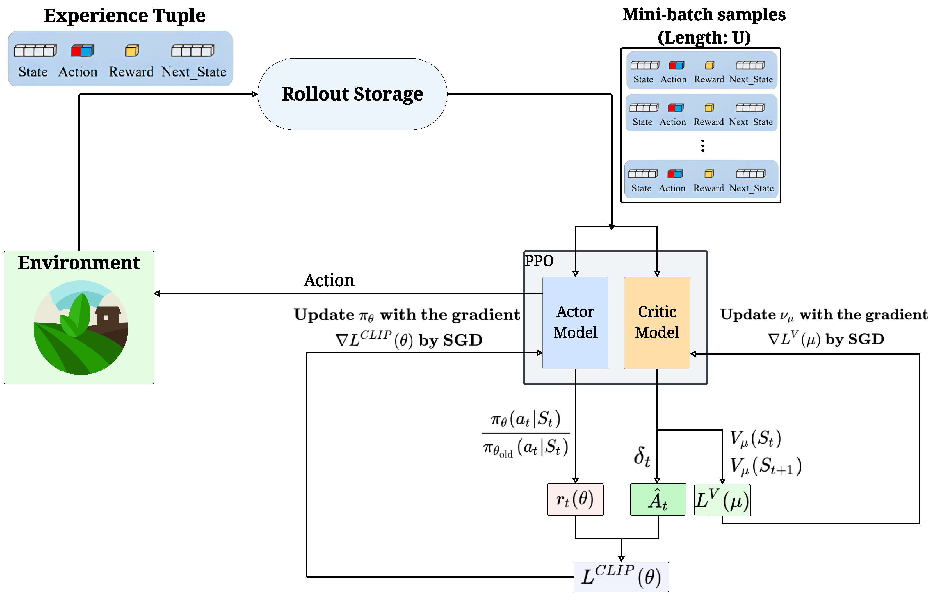
• Environment interaction and experience collection—Given the modeled environment E, the action model takes an action $a_t$ in E, obtaining in response from E the following experience tuple: $\langle s_t,a_t,r_t,s_{t+1}\rangle$, where $s_t$ is the current state, $a_t$ is the action taken, $r_t$ is the reward received by performing $a_t$ in $s_t$, and $s_{t+1}$ is the reached state. This interaction continues for a fixed number of steps, generating a sequence of experiences, also called a trajectory of experiences.
• Rollout storage (trajectory memory)—The sequence of collected experience tuples are temporarily stored in a component called rollout storage. This component acts as a buffer that holds the sequence of experiences generated by the agent’s current policy ${\pi }_{\theta }$. It is an essential element of the PPO because the algorithm uses this collected data for multiple learning updates before discarding them and collecting a new trajectory.
• PPO components: actor and critic models—The PPO block contains the two core learning models.
  • Actor model (or policy model): It can be considered as the agent’s decision-maker. It receives information about the current state $s_t$ and decides which action $a_t$ to take. Its goal is to develop a stochastic policy ${\pi }_{\theta }\left(a_t\right|s_t)$, which is essentially a set of rules or probabilities that dictate the best action for any given state. Indeed, given the state $s_t$ as input, it produces the probabilities of taking each different action $a_t$. The parameter $\theta$ represents the knowledge it has learned so far.
  • Critic model (or value model): This acts as the agent’s evaluator. It assesses how good a particular state $s_t$ is, or how good a particular action $a_t$ taken in a state $s_t$ is. It learns to estimate the expected future reward ($V_{\mu }\left(s_t\right)$) achievable from the current state $s_t$. The parameter $\mu$ represents the learned evaluation knowledge.
• Data preparation for learning—Once an iteration has been completed, the two models can be updated. This update exploits the data collected inside the rollout storage component and requires the computation of the following parameters:
  • Policy ratio $r_t\left(\theta \right)$: For each action $a_t$, the algorithm calculates the probability of taking that action under the current policy ${\pi }_{\theta }\left(a_t\right|s_t)$ and compares it to the probability under the old policy ${\pi }_{{\theta }_{old}}\left(a_t\right|S_t)$. This comparison produces the importance sampling ratio ($r_t\left(\theta \right)$), defined as follows:

    $$r_t\left(\theta \right)={\displaystyle \frac{{\pi }_{\theta }\left(a_t\right|s_t)}{{\pi }_{{\theta }_{\mathrm{old}}}\left(a_t\right|s_t)}}$$

    (1)
    This ratio is a key factor in PPO stability, ensuring that updates do not deviate too far from the old policy.
  • Temporal Difference (TD) error ${\delta }_t$: The estimates provided by the critic network are used to calculate the TD error, which measures the difference between the expected return and the actual value observed. It is typically calculated as:

    $${\delta }_t=r_t+\gamma ·V_{\mu }\left(s_{t+1}\right)-V_{\mu }\left(s_t\right)$$

    (2)

    where $\gamma$ is the discount factor used to modulate the role of future rewards with respect to the current one.
  • Advantage estimation ${\widehat{A}}_t$: Using the TD errors, the Generalized Advantage Estimation (GAE) is calculated. This provides a more accurate measure of how much better a chosen action was compared to the average expected outcome from that state. It is a crucial input for updating the actor model.
• Model updates (optimization)—The prepared data is then used to update both the actor and critic models. A batch of samples, referred to as mini-batch samples (length: U), is drawn from the rollout storage for these updates.
  • Critic model update: The objective of the critic model is to minimize its value loss, denoted as $L^V\left(\mu \right)$. This loss measures the squared difference between the predicted values ($V_{\mu }\left(s_t\right)$) and the actual returns. The parameter $\mu$ characterizing this network is then updated using its gradient, $\nabla L^V\left(\mu \right)$, typically through an optimization algorithm like Stochastic Gradient Descent (SGD).
  • Actor model update: The objective of the actor model is to minimize its clipped policy loss, denoted as $L^{CLIP}\left(\theta \right)$. This is the core of PPO. It uses the importance sampling ratio $r_t\left(\theta \right)$ and the advantage estimation ${\widehat{A}}_t$ to construct a loss function that encourages beneficial actions while preventing large, destabilizing changes to the policy. In particular, the clipping mechanism within this loss computation ensures that the ratio $r_t\left(\theta \right)$ always stays within a certain range. The simplified policy loss can be seen as:

    $$L^{CLIP}\left(\theta \right)=\min (r_t\left(\theta \right){\widehat{A}}_t,\mathrm{clip}(r_t\left(\theta \right),1-ϵ,1+ϵ){\widehat{A}}_t)$$

    (3)

    where $ϵ$ is the clipping hyperparameter. The parameter $\theta$ characterizing this network is updated using its gradient, $\nabla L^{CLIP}\left(\theta \right)$, typically through an optimization algorithm like SGD. An entropy bonus (not explicitly shown in the formula but often added) is also typically included to encourage exploration.

This cycle of interaction, experience collection, data preparation, and model updates is repeated iteratively, allowing the agent to continuously learn and improve its performance in the environment.

Given these preliminary notions, the following section formalizes the problem and describes the proposed solution.

2.2. Problem Formalization and Proposed Method

This section formalizes the problem introduced in Section 1 and describes the proposed solution.

Table 1. List of used symbols.

Symbol	Meaning
$\mathbb{T}$	temporal domain
$\mathcal{P}$	set of PoIs
V	set of nodes representing PoIs
E	set of edges between PoIs
$\mathcal{P}$	set of PoIs
$\mathcal{L}$	node labeling
$t_p$	time for measuring in $p\in \mathcal{P}$
$c_p$	time for charging in $p\in \mathcal{P}$
$\mathcal{E}$	edge labeling
$m_{ij}$	time for moving from $i\in \mathcal{P}$ to $j\in \mathcal{P}$
$e_{ij}$	energy consumed for moving from $i\in \mathcal{P}$ to $j\in \mathcal{P}$
$\gamma$	robot trajectory
$\mu$	measuring trajectory
$\xi$	charging trajectory
${\tau }_{\gamma }$	time for completing $\gamma$
x	contextual measure
$\delta =\langle d_1,\dots ,d_n\rangle$	contextual dimensions
$\rho =\langle w_1,\dots ,w_n\rangle$	context
$r(p,q)$	reward for going from p to q
$\varsigma$	charging level of the robot
ℓ	position of the robot
$\sigma (p,q)$	checks if $p=q$

reports the list of used symbols. Before dealing with such formalization, it is necessary to define the concept of temporal domain used in the following.

Definition 1

(Temporal Domain). A temporal domain $\mathbb{T}$ is a tuple $(T,\le )$, where T is a set of not-empty temporal instants and ≤ is an ordering relation on T [45].

In other words, a temporal domain $\mathbb{T}$ is a set of totally ordered time instants. A granularity is a mapping defined as follows.

Definition 2

(Temporal granularity). Given a temporal domain $\mathbb{T}$, the temporal granularity is a mapping G from the integers $\mathbb{Z}$ (set of indexes) to a subset of $\mathbb{T}$ such that:

1. 

If $i<j$ and $G\left(i\right)$ and $G\left(j\right)$ are not empty, then the elements of $G\left(i\right)$ are less than all the elements of $G\left(j\right)$.

2. 

If $i<k<j$ and $G\left(i\right)$ and $G\left(j\right)$ are not empty, then $G\left(k\right)$ is also not empty.

In other words, the granularity defines a partition of the temporal domain in elements that are considered indivisible units, called $\mathit{granules}$.

Time granularity can be defined as the resolution power of the temporal qualification of a statement. In this paper, we will consider only discrete temporal domains, and the minimum granularity is given by an interval of one minute. Therefore, a temporal duration or temporal interval will be measured as the number of minutes between two granules. For the purposes of this study, we consider only non-negative temporal intervals. Accordingly, we define a temporal interval as an element of the set $\mathbb{N}$, where $\mathbb{N}$ denotes the set of natural numbers including zero, following the standard algebraic definition [46].

The environment under investigation is characterized by the following underlying hypothesis, which will be formalized as a whole in Definition 3.

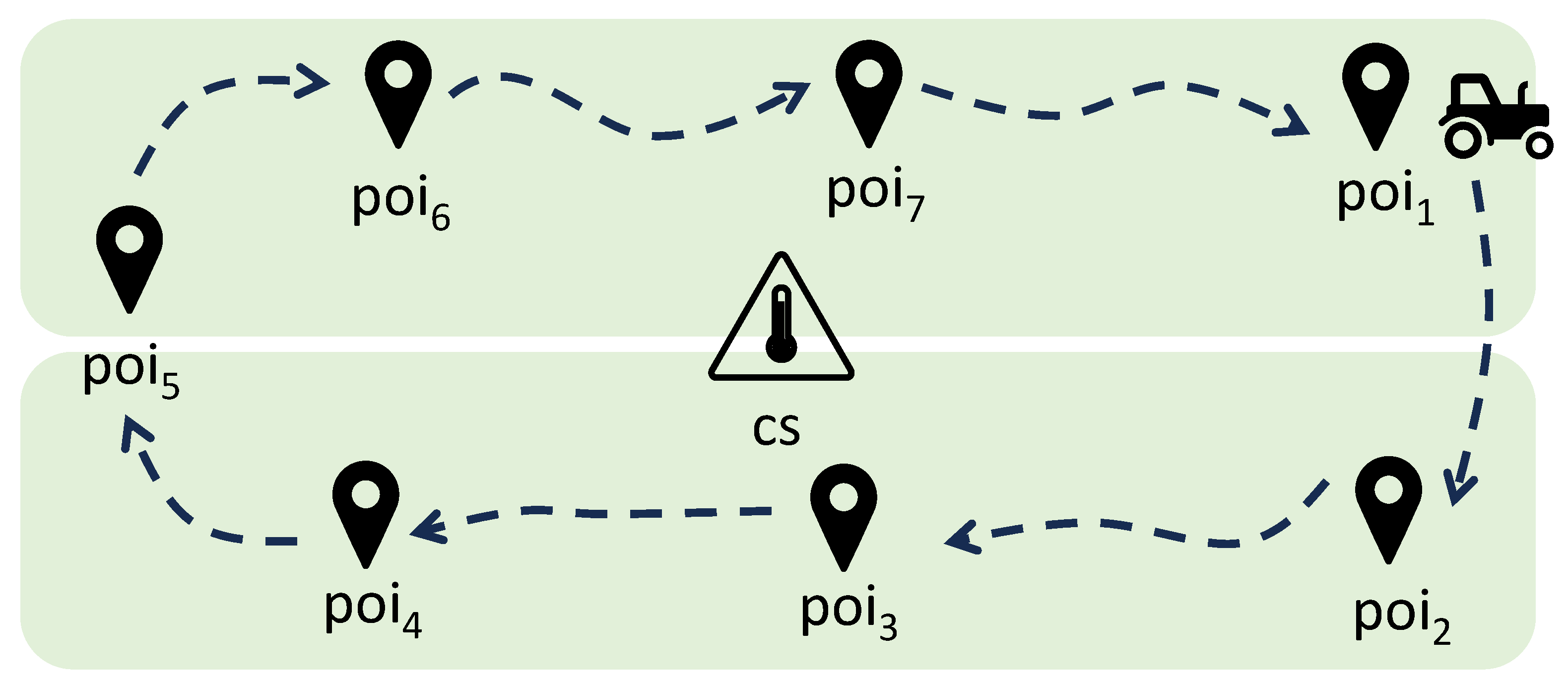
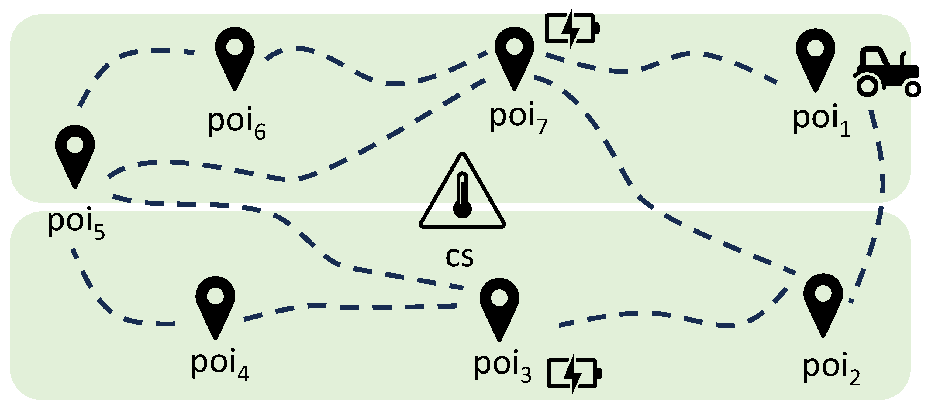
• An agricultural robot periodically describes a trajectory during its farming operations that potentially touches all elements of a set $\mathcal{P}$ of predefined and well-identified PoIs. The visit order is not predefined, and there are no precedence constraints. Moreover, some PoIs in $\mathcal{P}$ could be skipped during a specific trajectory.
• Each PoI $p\in \mathcal{P}$ could be reached directly or indirectly by passing through other PoIs, so there could be more than one path connecting the same pair of PoIs.
• There is no fixed direction in visiting PoIs; namely, the robot can go forward and backward among the PoIs.
• The robot is equipped with a device able to sample some climatic variables during the execution of its tasks. The measuring activity is done during farming operations. Therefore, we assume the presence of a function t, which returns for each PoI p the time required to complete the farming operations, including the measuring task. Since the assumed temporal granularity defines a resolution of one minute, the duration $t\left(p\right)$ for each $p\in \mathcal{P}$ becomes the number of minutes needed to complete the task.
• The movement from one PoI $p_1\in \mathcal{P}$ to another PoI $p_2\in \mathcal{P}$ requires some time, which is represented by a function m that returns for each pair of PoIs the amount of time needed to perform such a movement. Again, since we consider a temporal granularity of one minute, m returns the number of minutes needed to complete such movement.
• The robot has a limited amount of energy charge, which is also consumed by moving among PoIs, so it needs to be recharged periodically. For the sake of simplicity, we assume that the available and consumed energy is expressed as an integer representing the battery life in terms of minutes.
• Some PoIs contain a charging station in which the robot battery can be charged. The charging activity takes some time to complete, and it does not overlap with farming/measuring operations. For the sake of simplicity, we assume that the charging time depends only on the current capabilities of the charging station, but the model is general enough to include a more complex function that also depends on the charging conditions, like the current battery level. In other words, in practical scenarios, the charging time will depend on the battery level at the moment of recharge, and the robot may require less time to recharge if the battery is not fully depleted. Future work could focus on incorporating a dynamic charging time model based on the robot’s actual battery level, enabling more accurate energy management. Integrating variable charging times into the trajectory planning algorithm will improve scheduling efficiency and leads to more realistic and effective operational strategies. In any case, the time required to complete a charging operation is represented by the number of minutes needed to complete it.
• The farming/measuring operations are orthogonal to charging operations, and a robot can stop in a PoI to either measure, charge, or do both.

An environment characterized by these hypotheses can be formally represented through a graph where the nodes represent PoIs, and the edges are the paths connecting them.

Definition 3

(Environment Graph). The environment characterizing the problem at hand can be described as a bi-directed labeled graph $G=(V,E,\mathcal{L},\mathcal{E})$, where:

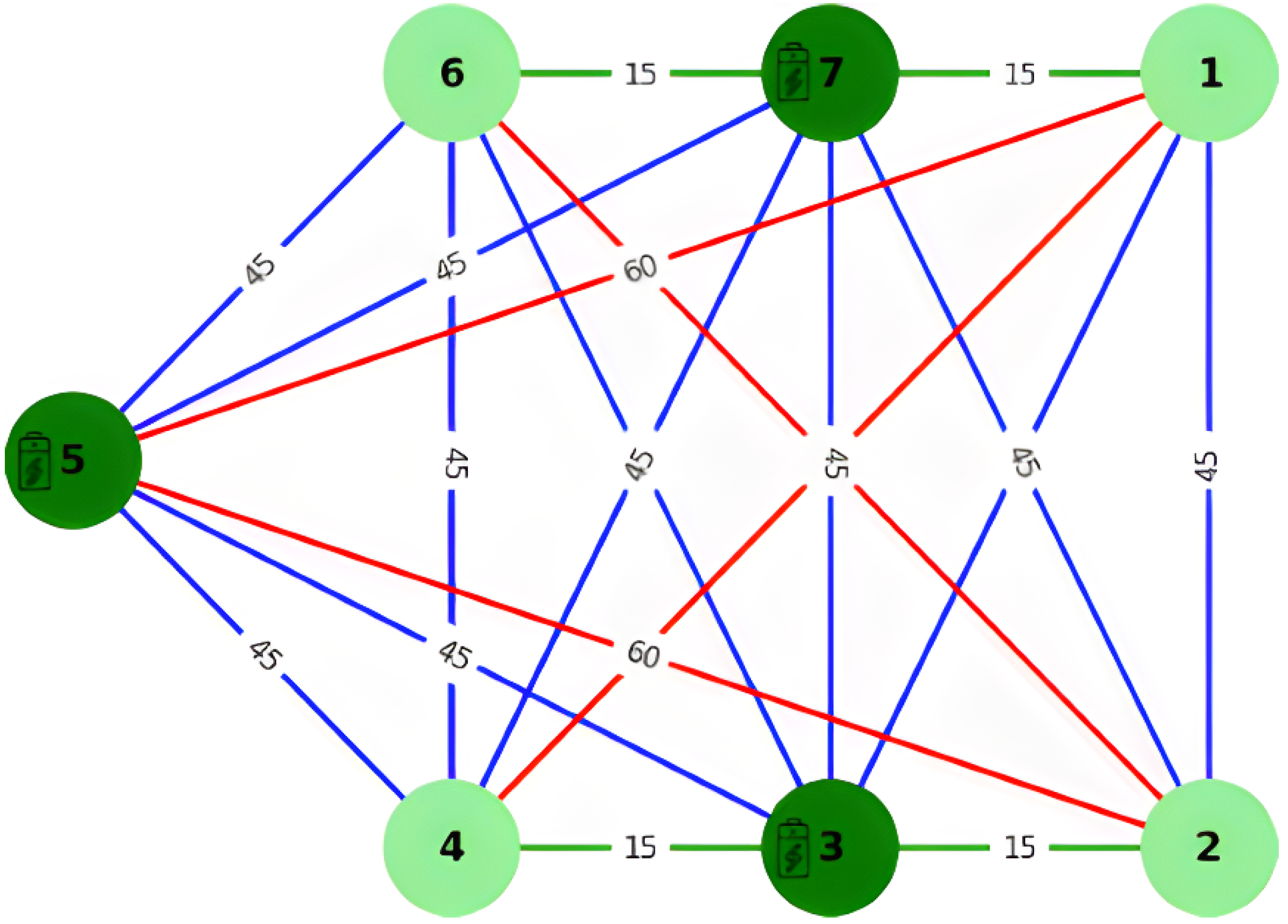
• V is the set of nodes representing the PoIs.
• $E\subseteq \left\{\right(u,v):u,v\in V,u\ne v\}$ is the set of bi-directional edges representing the paths connecting the nodes.
• $\mathcal{L}:V\to \mathcal{P}\times {\mathbb{N}}^{+}\times \mathbb{N}$ is a labeling function assigning a label $\langle p,t_p,c_p\rangle$ to each node $u\in V$, defined as follows:

  –

  $p\in \mathcal{P}$ is the identifier of the PoI.

  –

  $t:\mathcal{P}\to {\mathbb{N}}^{+}$ is the function that represents the time required to complete the measuring task together with the farming task inside p. The notation $t_p$ is used in place of $t\left(p\right)$ for not cluttering the notation,

  –

  $c:\mathcal{P}\to \mathbb{N}$ indicates whether a given PoI p contains a charging station, i.e., $c_p=0$ means that p does not contain a charging station, while $c_p>0$ represents the time required for the charging operation.

• $\mathcal{E}:E\to {\mathbb{N}}^{+}\times {\mathbb{N}}^{+}$ is a function that assigns a label $\langle m_{u,v},e_{u,v}\rangle$ to each edge $e\in E$ as follows:

  –

  $m:\mathcal{E}\to {\mathbb{N}}^{+}$ is the function that represents the time required by the robot to move between two adjacent PoIs. In the following, to not clutter the notation, we will use $m_{u,v}$ to denote the time spent to move from PoI $p_u$ to PoI $p_v$. Since the edges are bi-directional, we assume that $m_{u,v}=m_{v,u} \forall (u,v)\in \mathcal{E}$

  –

  $e:\mathcal{E}\to {\mathbb{N}}^{+}$ is the function that represents the energy required by the robot to move between two adjacent PoIs, i.e., $e_{u,v}$ is the energy to be consumed to move from PoI $p_u$ to PoI $p_v$. Since the edges are bi-directional, we assume that $e_{u,v}=e_{v,u} \forall (u,v)\in \mathcal{E}$

As an instance, Figure 5 reports the graph notation for the environment introduced in Figure 3. In particular, three charging PoIs can be identified (i.e., $po{i}_3$, $po{i}_5$, and $po{i}_7$). The time required to reach each PoI from another one can be different (i.e., from 15 to 45 min), while the time to be spent in each PoI for measuring is 15 min. In this paper, we assume that the energy consumed to traverse an edge has been considered proportional to the travel time with a unitary coefficient so that its magnitude corresponds to the travel time. However, more complex formulations can be adopted without altering the notation.

Given the definition of the environment graph, we can derive the definitions of robot trajectory, measurement trajectory, and charging trajectory.

Definition 4

(Robot trajectory). Given an environment graph $G=(V,E,\mathcal{L},\mathcal{E})$ built starting from a set of PoIs $\mathcal{P}={\left\{p_i\right\}}_{i=1}^n$ inside a greenhouse, we define a robot trajectory as the ordered sequence $\gamma =\langle p_1,\dots ,p_n\rangle$ of PoIs in which the robot stops for performing a measurement of the climatic variables of interest (together with its farming tasks) or for charging.

Definition 5

(Measurement trajectory). Given a robot trajectory $\gamma =\langle p_1,\dots ,p_n\rangle$, a measurement trajectory is a sub-sequence $\mu =\langle p_i,\dots ,p_k\rangle \subseteq \gamma$ composed only of the PoIs in γ where the robot stops to perform only a measurement.

Definition 6

(Charging trajectory). Given a robot trajectory $\gamma =\langle p_1,\dots ,p_n\rangle$, a charging trajectory is a sub-sequence $\chi =\langle p_j,\dots ,p_h\rangle \subseteq \gamma$ composed only of the PoIs in γ where the robot stops for charging.

Given a robot trajectory $\gamma$ together with its related measurement $\mu$ and charging $\chi$ sub-sequences, the time ${\tau }_{\gamma }$ required to complete the entire trajectory $\gamma$ can be computed as:

$${\tau }_{\gamma }=\sum _{i\in \mu }{t}_i+\sum _{j\in \chi }{c}_i+\sum _{i,j\in \gamma }{m}_{ij}$$

(4)

where $i\in \mu$ or $i\in \chi$ identifies the index of a PoI inside the measurement or charging trajectory, respectively, while $i,j\in \gamma$ identifies a pair of consecutive PoIs in $\gamma$.

With reference to the example in Figure 2, a possible robot trajectory could be represented by the sequence $\gamma =\langle p_1,p_2,p_7,p_5,p_6\rangle$, where the measuring trajectory $\mu$ might correspond to $\gamma$, since we may decide to take a measurement in each touched PoI, while the charging trajectory $\chi$ might be composed of $p_7$ only, since the robot might need only one charging operation to complete the whole trajectory.

Given a set of PoIs $\mathcal{P}$ that the robot should periodically sample, the aim of this paper is to identify the optimal trajectory while considering the battery level of the robot.

As already discussed in Section 1, the choice of the sequence of PoIs to include in the robot trajectory $\gamma$ is not fixed, and it can change depending on the particular conditions (i.e., context) in which the measurements are performed. For this reason, we need to define the notion of measurement context as follows.

Definition 7

(Context). Given a measurement $x\in \mathbb{R}$ performed on a greenhouse at a given temporal instant $i\in \mathbb{T}$, we define the context ρ in which the measurement is performed as a tuple of values of dimensions $\delta =\langle d_1,\dots ,d_n\rangle$ as follows: $\rho =\langle w_1,\dots ,w_n\rangle$, where each $w_h\in \rho$ is the value of the contextual dimension $d_h\in \delta$.

For our problem, three main types of contextual dimensions are of interest: (i) the time instant i in which the measurement is performed, (ii) the general climatic conditions inside the greenhouse, represented by the values collected by the central climatic station $cs$ in Figure 3, (iii) the relative position of a PoI with respect to the current position of the robot, which is important in terms of travel time and required charge to get there, (iv) the battery level of the robot and its position relative to the nearest charging station, which is important to choose next PoI to visit.

With reference to the DRL terminology, the agent is represented by the agricultural robot, and the notion of state is represented by its current node occupied inside the environment graph, together with the specific current context. For our purposes, the robot can be formalized as follows:

Definition 8

(Robot agent). The robot agent is a tuple $\langle \varsigma ,\ell \rangle$ where $\varsigma :\mathbb{T}\to \mathbb{N}$ is a function returning for each temporal instant $i\in \mathbb{T}$ the charging level of the robot battery, while $\ell :\mathbb{T}\to V$ is a function returning for each temporal instant $i\in \mathbb{T}$ the PoI $p\in \mathcal{P}$ currently occupied by the robot.

The final ingredient we need to formalize is the notion of reward used during the learning process to provide prompt feedback and encourage the agent to take the most suitable action.

Definition 9

(Reward). Given a PoI $p\in \mathcal{P}$ representing the current position $\ell \left(i\right)$ of the robot at time $i\in \mathbb{T}$, the reward associated with stopping in a subsequent PoI $q\in \mathcal{P}$ is defined as follows:

$$r(p,q)={\Delta }_q(i+m_{pq})-\sigma (p,q)-e_{pq}-{\Gamma }_{pq}\left(t\right)$$

(5)

This reward function is designed with two main priorities:

1. 

Promote safety and avoid critical conditions

• Avoiding Stagnation: A significant penalty is applied if the agent stays in the same place. This is captured by $\sigma (p,q)$ in Equation (5), which checks if p and q represent the same PoI.
• Battery Management: Severe penalties are given for critical battery levels (i.e., it is too low to reach a charger, or it is empty). Conversely, a positive reward is provided for successfully reaching a charging station, especially when the battery is low. A penalty is also applied when the battery drops below a warning threshold, prompting the agent to seek charging early. These considerations about the battery level are captured by the term ${\Gamma }_{pq}\left(t\right)$ in Equation (5), which is based on the value returned by the function $\varsigma \left(t\right)$ in Definition 8.

2. 

Performance Optimization

• Temperature Considerations: The reward for visiting a new location is based on the difference between the temperature that was previously measured or estimated there and the temperature that is expected at that location when the agent arrives. A larger difference in temperature indicates a greater importance of visiting that specific location, thus resulting in a higher reward for its selection. This is captured by the term ${\Delta }_q(i+m_{pq})$ in Equation (5).
• Time and Resource Efficiency: The agent is penalized for the time taken for actions and the resources consumed, encouraging faster and more efficient operations. This is captured by the term $e_{pq}$ in Equation (5), which measures the energy required to move from p to q.

This reward structure ensures that the agent prioritizes safety while simultaneously learning to perform its tasks efficiently and effectively. It will be used in each state to identify the next best action to perform in the long term, namely the PoI to choose as the following stop in the trajectory. Based on this, the best trajectory is defined as the best sequence of stops to consider in the current context. Notice that, since there can be more than one path connecting the same pair of PoIs, we use Dijkstra’s algorithm to find the shortest path between all pairs of PoIs.

The result produced by the proposed approach is the sequence of PoIs in which the robot should stop to either perform measurements, recharge, or both.

2.3. Implementation Details

The full source code (Version 1.0) is available in a GitHub repository at https://github.com/AshrafSharifi/RechargeableRobot-Trajectory-PPO (accessed on 28 June 2025). In the experiments, we use the PPO implementation provided by the CleanRL library available at https://github.com/vwxyzjn/cleanrl (accessed on 28 June 2025). The proposed PPO agent is implemented in Python (Version 3.10.14) using PyTorch Version 2.0.1 (CUDA 11.7 build). The architecture follows an actor–critic paradigm, where both policy and value function approximators are neural networks trained concurrently. The following subsections provide additional details about the implementation.

2.3.1. Framework and Libraries

The implementation is based on PyTorch, utilizing modules such as torch.nn for network definition, torch.optim for optimization, and torch.distributions.Categorical for sampling actions in discrete action spaces. Additional supporting libraries include NumPy, Pandas, and Pickle for data manipulation and serialization, as well as TensorBoard for the logging of training metrics via torch.utils.tensorboard.SummaryWriter.

2.3.2. PPO Configuration

The implementation of PPO requires the definition of the two components of the actor–critic architecture described in Figure 4 of Section 2.1. As described in the literature, these two neural networks can have different architectures and complexities. In the proposed work, we used the following two neural network architectures: the actor network is a fully connected network with ReLU activation, containing two hidden layers with 128 and 64 units, respectively. Similarly, the critic network is also a fully connected network with ReLU activation, but in this case, there are three hidden layers with 32, 16, and 8 units, respectively, and a single output for error value estimation.

The agent adheres to the canonical PPO formulation, with several implementation-specific enhancements:

• Policy and Value Networks: The actor model outputs logits for a discrete action space, while the critic model estimates the scalar state value $V\left(s\right)$. Orthogonal initialization is used for all layers.
• Generalized Advantage Estimation (GAE): Employed to compute advantages, reduce variance, and improve learning stability.
• Clipped Surrogate Objective: The policy loss is calculated using the PPO clipped objective to ensure conservative policy updates.
• Entropy Regularization: An entropy bonus is added to the loss function to promote exploration.
• Gradient Clipping: Applied to all gradients with a configurable maximum norm to maintain stability.
• Learning Rate Annealing: The learning rate decays linearly over the training iterations.

2.3.3. Environment and Reward Shaping

A custom simulation environment is used, featuring a structured state space including sensor location, battery level, and temperature-related features. The reward function is shaped by the weighted components described in Equation (5). The corresponding weights are configurable for task-specific tuning.

2.3.4. Training Protocol

Training is conducted in an on-policy manner. Trajectories are collected for a fixed number of steps per iteration, and multiple epochs of minibatch updates are performed. No replay buffer is used. Model checkpoints are saved using PyTorch native serialization, and evaluation is performed in deterministic mode.

2.3.5. PPO Hyperparameters

All major hyperparameters are chosen based on standard practices in the literature (e.g., CleanRL documentation) to ensure stable and efficient learning. Specifically, we use a learning rate of $2.5\times {10}^{-4}$, a discount factor $\gamma =0.99$, and GAE parameter $\lambda =0.95$. The surrogate loss uses a clipping coefficient of $0.1$, with four update epochs and four minibatches per iteration. To encourage exploration, we apply an entropy regularization coefficient of $0.01$, while the value function loss is weighted by $0.5$. Gradient clipping is applied with a maximum norm of $0.5$, and the value loss is clipped to enhance critic stability. These settings are consistent with widely accepted PPO implementations and were found to work well in our environment without requiring additional tuning.

3. Results and Discussion

3.1. Application Setup

The solution introduced in the previous section has been validated with the data collected in two adjacent greenhouse tunnels located near Verona (${45}^{\circ }$${20}^{\prime }$${25.9}^{″}$ N ${11}^{\circ }$${05}^{\prime }$${12.3}^{″}$ E and ${45}^{\circ }$${20}^{\prime }$${47.13}^{″}$ N ${11}^{\circ }$$1^{\prime }$${46.4}^{″}$ E, respectively) in Northeastern Italy from late August 2021 to early July 2022. This region experiences warm and humid conditions during the summer months, while winters are relatively mild to moderately cold.

Each tunnel is $275.6 {\mathrm{m}}^2\hspace{1em}(50 \mathrm{m}\times 5.3 \mathrm{m})$ northeast–southwest oriented and covered with transparent plastic film. It represents the module of a multispan greenhouse structure typical of this geographical area (Figure 6). As complementary information, before crop transplanting, the soil was tilled and subsequently mulched with a semitransparent green polyethylene film. For the duration of the experiment, both farms changed cultivated crops according to the season: the first farm cycled through eggplants, then lettuce, and finally cucumbers; the second one cycled through tomatoes, lettuce, and finally, eggplants.

3.2. Experimental Results and Discussion

The real configuration of the mentioned greenhouse is essentially an enrichment of the graph in Figure 5, in which seven PoIs are present together with a climatic station by Evja srl (https://www.evja.eu accessed on 28 June 2025) placed in the center. Figure 7 provides a simplified notation for this environment graph. In particular, to not clutter the graph, we use the following convention: each edge $(p,q)$ reports only the time required to reach PoI q from PoI p ($m_{pq}$); the required energy is assumed to be measured in consumption minutes and is considered numerically equal to the travel time. A small battery icon identifies the nodes containing a charging station, namely $p_3$, $p_5$, and $p_7$ in Figure 7; both measurement time ($t_p$) and charging time ($c_p$) are set to 15 min for each PoI p.

Considering this configuration and the historical data containing the context in which the measurement trajectories have to be performed, we compute the best trajectory by using the proposed PPO approach described in Section 2.2. Figure 8 illustrates an example of its functioning, where for each step, the start and end PoI are identified by a green box indicating the timestamp of the starting time, the remaining battery level, and the reward associated with this movement action. The robot starts in $p_5$ with a full battery level of 300; in this situation, the algorithm identifies the best action to perform the movement towards $p_4$ (Step 1), where the robot arrives after 45 min and stays for 15 min, consuming a total of 60 units of energy and obtaining a reward of 19.28. Similarly, in Step 2, the robot has enough battery to reach each PoI without any problem, and the algorithm identifies the movement towards $p_1$ as the best action. In the following Step 3, $p_6$ is the best PoI to visit, but since there is no direct path from $p_1$ to $p_6$, the robot also needs to traverse $p_7$, but without stopping in it for measuring or for charging. Indeed, the end time reported in $p_6$ is 45 min after the departure from $p_1$: 30 min for traveling and 15 min in $p_6$ for measuring and other farming tasks. Conversely, in Step 4, the algorithm decides that the robot needs to be recharged (its battery level is below a threshold limit of 140). Therefore, the next PoI to visit should be identified among $p_3$, $p_5$, and $p_7$, because they all contain a charging station. In particular, the algorithm chooses $p_3$ since its reward is greater than that of the other two: even if it is further away than $p_7$, it is more interesting for the estimated temperature difference component. It is worth noting that, in this case, the reward associated with the action is much greater than the other, as the robot can stop in the same PoI to perform two operations, i.e., measuring and charging. In other words, in this trajectory, $p_3$ will become part of both the measuring and the charging sub-trajectories.

The proposed approach could be applied to various environments with different configurations, thus leading to different trajectories. Figure 9 compares the results produced starting from the same situation (i.e., initial PoI, timestamp and battery level) but in a slightly different environment regarding the available connections between PoIs. In the original environment, the suggested trajectory was $p_1$, $p_6$ (through $p_7$), then $p_3$. Conversely, when removing the edge from $p_7$ to $p_6$, it determines that the best PoI to visit after $p_1$ becomes $p_3$, followed by $p_6$. In other words, the order of visits between $p_6$ and $p_3$ has been switched, since $p_3$ is now in the shortest path towards $p_6$, and the robot can exploit this situation.

The trajectories obtained using the proposed approach in the considered real-world scenario have been evaluated with respect to two aspects: (i) the ability to produce robot trajectories that allow for the collection of a meaningful sequence of measurements for subsequent tasks (i.e., the quality of the measuring sub-trajectories), (ii) the effects of the proposed trajectories on the battery levels and autonomy of the robot (i.e., the quality of the charging sub-trajectories).

Quality of the measuring sub-trajectories—

Table 2. Comparison between the estimation errors of the model in [15] when it is trained with the trajectories produced using: (i) the proposed approach, (ii) the previous approach in [18], (iii) the continuous complete itinerary used in [17].

PoI	Proposed Work					Previous Work [18]					Baseline Method [17]
	# Visits	MAPE%	MAE	MSE		# Visits	MAPE%	MAE	MSE		# Visits	MAPE%	MAE	MSE
1	419	5.1	0.93	2.2		343	7.7	1.3	4.4		560	8.8	1.4	4.1
2	395	5.5	1.0	2.5		241	5.7	1.0	2.6		560	6.1	1.2	2.6
3	396	5.6	1.0	2.6		323	7.2	1.3	4.6		520	8.6	1.5	4.7
4	356	5.9	1.2	3.2		53	7.3	1.3	4.6		560	8.3	1.5	4.8
5	383	5.2	1.0	2.6		62	6.8	1.3	3.6		520	7.5	1.4	3.8
6	384	5.8	1.2	3.7		87	8.2	1.6	6.0		560	8.3	1.6	5.3
7	405	5.1	1.0	2.5		161	6.8	1.3	4.7		560	6.9	1.3	3.7
All	2738	5.4	1.1	2.7		1270	7.1	1.3	4.3		3840	7.8	1.4	4.1

reports, for each PoI, the number of times it has been visited during the identified trajectories (# Visits) together with the prediction accuracy (in terms of MAPE, MAE, and MSE, respectively) of the Deep Learning (DL) model [15] trained to estimate future temperature values in this PoI. We compare the prediction accuracy of the DL model when it is trained with three different kinds of historical data: (i) the ones collected through the trajectories determined using the approach proposed in this paper, (ii) the ones collected using our previous approach [18], which does not consider charging requirements and allows only to skip some PoIs inside direct trajectories, and (iii) the ones collected by always performing complete trajectories, as suggested in [17] (baseline).

The results in Table 2 show that the proposed approach outperforms both previous methods since it allows for the production of a training set with which the estimation model in [15] can achieve a better accuracy (i.e., lower error). This holds both in the case of a single model for each PoI and of a unique model trained with the data of all PoIs altogether. Another aspect to notice is that this increased accuracy is connected with a greater number of visits to each single PoI in the same amount of time. This effect was also visible in [18], where the time to complete the fixed trajectory could be reduced by skipping the measurement activity in some PoIs, but in the current approach, it becomes more evident due to the robot’s increased flexibility to move through each PoI. As a result, within a short time, the robot could collect more measurements at important PoIs by visiting them multiple times.

Quality of the charging sub-trajectories—As a final experiment, we evaluate the robot’s battery level during the suggested trajectories. First, we performed tests to examine the impact of reducing the initial battery capacity on the number of times the robot had to stop for charging activities. The results showed that when the robot’s full charge was set to 300 units, it made 257 stops at charging stations during all the considered 1656 trajectories. However, when the full charge was reduced to 150 units, the number of stops increased significantly to 406. Secondly, considering an initial battery level of 300 and the trajectories produced by the method in [18], we examined how many times the robot is located at PoIs equipped with a charging station during a critical moment (i.e., its battery level is less than the threshold) and so can solve this situation without running out of charge in the middle of a trajectory. Our experiment shows that, with the previous approach, in approximately 168 cases, the robot needed to be charged, whereas in 83 of these cases, it was not located at PoIs containing a charging station.

4. Conclusions

Agricultural robots will be applied in farming tasks, both outdoors and inside greenhouses. This paper aims at integrating their management and with the possibility of exploiting them for additional services, e.g., to provide complete and detailed climate mapping of the environment, which is particularly important to ensure and improve the health and growth of plants.

We propose a novel solution for the identification of the best trajectory to be performed by an agricultural robot with the aim of adequately balancing measurement accuracy and energy autonomy. This method is based on the application of reinforcement learning together with the Proximal Policy Optimization (PPO) algorithm for the reward function, which takes into consideration both the importance of each PoI in the accuracy of the greenhouse climate mapping and the need to recharge the robot when its battery goes below a given threshold level. For doing so, the environment has been formalized through a labeled bi-directional graph, in which nodes represent PoIs where measurements and re-charge can take place, and edges are the possible paths between them. We also formalized the technological features of the robot, i.e., the speed and the consumption rate.

This representation, together with the usage of historical data to train the PPO algorithm, represents an original example of a mixed model-driven and data-driven approach in the field of precision agriculture. More features related to the environment and the robot could be added in the future.

Climate monitoring deserves particular attention. This process, being data-driven, is not statically predefined; thus, it represents an example of active sensing. Furthermore, if we assume that temperature evolution follows a hidden physical behavior, its continuous observation to predict future values can be considered as an attempt to build its model, which then is used to decide the robot’s actions, thus fully recalling the concept of digital twin. Future work may consider more complex and interesting dynamic models, such as those of plants and pathogens, so that the decision of the robot’s actions could be not only restricted to trajectory planning but also to full agronomic tasks.

The proposed approach was tested using data for a real-world scenario regarding a greenhouse in Verona, a city in Northeast Italy. The obtained results were compared with two baselines in [17,18], demonstrating the goodness of the proposed approach. In particular, the production of the training set was improved, since it allows the prediction model to produce temperature estimations that were, overall, about 2–2.5% more accurate compared to the ones obtained with the training sets produced by the two baselines. At the same time, since the proposed approach also takes into consideration the energy consumption and the charging level, it allows for a reduction of the number of stops by carefully predicting their need and preventing unexpected stopping.

Relative to the modeling of the robot’s power consumption and energy management, an interesting extension of the present work will be to incorporate a more realistic and flexible model of the recharging time that depends on the robot’s actual battery level at the time of recharge. Incorporating a dynamic charging time in future work would enable more precise energy management and improve trajectory planning, resulting in better scheduling efficiency and greater robot autonomy. We believe that this extension would bring the model closer to practical, real-world operation.

Moreover, extending the proposed approach to support multiple agricultural robots working together is a promising direction for future research. By coordinating their movements, the robots could cover more ground in less time and collect data more efficiently. This scenario would make the system more scalable and better suited for larger greenhouses or even open-field environments.

References

1. Revathi, S.; Sivakumaran, N.; Radhakrishnan, T. Design of solar-powered forced ventilation system and energy-efficient thermal comfort operation of greenhouse. Mater. Today Proc. 2021, 46, 9893–9900. [Google Scholar] [CrossRef]
2. Jolliet, O. HORTITRANS, a model for predicting and optimizing humidity and transpiration in greenhouses. J. Agric. Eng. Res. 1994, 57, 23–37. [Google Scholar] [CrossRef]
3. Van Pee, M.; Janssens, K.; Berckmans, D.; Lemeur, R. Dynamic Measurement and Modelling of Climate Gradients Around a Plant for mIcro-Environment Control; Number 456 in Acta Horticulturae; International Society for Horticultural Science: The Hague, The Netherlands, 1998; pp. 399–406. Available online: https://www.actahort.org/books/456/456_48.htm (accessed on 28 June 2025).
4. Zhao, Y.; Teitel, M.; Barak, M. SE—Structures and Environment: Vertical Temperature and Humidity Gradients in a Naturally Ventilated Greenhouse. J. Agric. Eng. Res. 2001, 78, 431–436. [Google Scholar] [CrossRef]
5. Roy, J.; Boulard, T.; Kittas, C.; Wang, S. PA—Precision Agriculture: Convective and Ventilation Transfers in Greenhouses, Part 1: The Greenhouse considered as a Perfectly Stirred Tank. Biosyst. Eng. 2002, 83, 1–20. [Google Scholar] [CrossRef]
6. Kittas, C.; Bartzanas, T.; Jaffrin, A. Temperature Gradients in a Partially Shaded Large Greenhouse equipped with Evaporative Cooling Pads. Biosyst. Eng. 2003, 85, 87–94. [Google Scholar] [CrossRef]
7. Chen, C. Prediction of longitudinal variations in temperature and relative humidity eor evaporative cooling greenhouses. Agric. Eng. J. 2003, 12, 143–164. [Google Scholar]
8. Kittas, C.; Bartzanas, T. Greenhouse microclimate and dehumidification effectiveness under different ventilator configurations. Build. Environ. 2007, 42, 3774–3784. [Google Scholar] [CrossRef]
9. Bojacá, C.R.; Gil, R.; Cooman, A. Use of geostatistical and crop growth modelling to assess the variability of greenhouse tomato yield caused by spatial temperature variations. Comput. Electron. Agric. 2009, 65, 219–227. [Google Scholar] [CrossRef]
10. Lopez-Martinez, J.; Blanco, J.; Perez, J. Distributed network for measuring climatic parameters in heterogeneous environments: Application in a greenhouse. Comput. Electron. Agric. 2018, 145, 105–121. [Google Scholar] [CrossRef]
11. Hamrita, T. A wireless sensor network for precision irrigation in Tunisia. Int. J. Distrib. Sens. Netw. 2005, 1, 67–74. [Google Scholar]
12. Teitel, M.; Wenger, E. Air exchange and ventilation efficiencies of a non-span greenhouse with one inflow and one outflow through longitudinal side openings. Biosyst. Eng. 2014, 119, 98–107. [Google Scholar] [CrossRef]
13. Pahuja, R. An intelligent wireless sensor and actuator network system for greenhouse microenvironment control and assessment. J. Biosyst. Eng. 2017, 42, 23–43. [Google Scholar] [CrossRef]
14. Rosas, J.; Palma, L.B.; Antunes, R.A. An Approach for Modeling and Simulation of Virtual Sensors in Automatic Control Systems Using Game Engines and Machine Learning. Sensors 2024, 24, 7610. [Google Scholar] [CrossRef] [PubMed]
15. Brentarolli, E.; Migliorini, S.; Quaglia, D.; Tomazzoli, C. Mapping Micro-Climate in a Greenhouse Through a Context-Aware Recurrent Neural Network. In Proceedings of the 2023 IEEE Conference on AgriFood Electronics (CAFE), Torino, Italy, 25–27 September 2023; pp. 113–117. [Google Scholar] [CrossRef]
16. Tomazzoli, C.; Brentarolli, E.; Quaglia, D.; Migliorini, S. Estimating Greenhouse Climate Through Context-Aware Recurrent Neural Networks Over an Embedded System. IEEE Trans. AgriFood Electron. 2024, 2, 554–562. [Google Scholar] [CrossRef]
17. Brentarolli, E.; Migliorini, S.; Quaglia, D.; Tomazzoli, C. Greenhouse Climatic Sensing through Agricultural Robots and Recurrent Neural Networks. In Proceedings of the 2023 IEEE International Workshop on Metrology for Agriculture and Forestry, Pisa, Italy, 6–8 November 2023. [Google Scholar]
18. Sharifi, A.; Migliorini, S.; Quaglia, D. Optimizing the Trajectory of Agricultural Robots in Greenhouse. In Proceedings of the 8th International Conference on Control, Automation and Diagnosis, ICCAD 2024, Paris, France, 15–17 May 2024. [Google Scholar]
19. Akyildiz, I.; Su, W.; Sankarasubramaniam, Y.; Cayirci, E. Wireless sensor networks: A survey. Comput. Netw. 2002, 38, 393–422. [Google Scholar] [CrossRef]
20. Gonda, L.; Cugnasca, C. A Proposal of Greenhouse Control Using Wireless Sensor Networks. In Proceedings of the Computers in Agriculture and Natural Resources—Proceedings of the 4th World Congress, Orlando, FL, USA, 24–26 July 2006. [Google Scholar] [CrossRef]
21. Chaudhary, D.; Nayse, S.; Waghmare, L. Application of Wireless Sensor Networks for Greenhouse Parameter Control in Precision Agriculture. Int. J. Wirel. Mob. Netw. 2011, 3, 140–149. [Google Scholar] [CrossRef]
22. Srbinovska, M.; Gavrovski, C.; Dimcev, V. Environmental parameters monitoring in precision agriculture using wireless sensor networks. J. Clean. Prod. 2015, 88, 297–307. [Google Scholar] [CrossRef]
23. Guzmán, C.H.; Carrera, J.L.; Durán, H.A.; Berumen, J.; Ortiz, A.A.; Guirette, O.A.; Arroyo, A.; Brizuela, J.A.; Gómez, F.; Blanco, A.; et al. Implementation of Virtual Sensors for Monitoring Temperature in Greenhouses Using CFD and Control. Sensors 2019, 19, 60. [Google Scholar] [CrossRef]
24. Davis, P. A technique of adaptive control of the temperature in a greenhouse using ventilator adjustments. J. Agric. Eng. Res. 1984, 29, 241–248. [Google Scholar] [CrossRef]
25. Sánchez-Molina, J.; Rodríguez, F.; Guzmán, J.; Arahal, M. Virtual sensors for designing irrigation controllers in greenhouses. Sensors 2012, 12, 15244–15266. [Google Scholar] [CrossRef]
26. Roldán, J.; Joosen, G.; Sanz, D.; del Cerro, J.; Barrientos, A. Mini-UAV based sensory system for measuring environmental variables in greenhouses. Sensors 2015, 15, 3334–3350. [Google Scholar] [CrossRef] [PubMed]
27. Pawlowski, A.; Guzman, J.; Rodríguez, F.; Berenguel, M.; Sánchez, J.; Dormido, S. Simulation of greenhouse climate monitoring and control with wireless sensor network and event-based control. Sensors 2009, 9, 232–252. [Google Scholar] [CrossRef] [PubMed]
28. Lin, B.; Recke, B.; Knudsen, J.K.; Jørgensen, S.B. A systematic approach for soft sensor development. Comput. Chem. Eng. 2007, 31, 419–425. [Google Scholar] [CrossRef]
29. Prasad, V.; Schley, M.; Russo, L.P.; Wayne Bequette, B. Product property and production rate control of styrene polymerization. J. Process Control 2002, 12, 353–372. [Google Scholar] [CrossRef]
30. Park, S.; Han, C. A nonlinear soft sensor based on multivariate smoothing procedure for quality estimation in distillation columns. Comput. Chem. Eng. 2000, 24, 871–877. [Google Scholar] [CrossRef]
31. Radhakrishnan, V.; Mohamed, A. Neural networks for the identification and control of blast furnace hot metal quality. J. Process Control 2000, 10, 509–524. [Google Scholar] [CrossRef]
32. Reichrath, S.; Davies, T. Using CFD to model the internal climate of greenhouses: Past, present and future. Agronomie 2002, 22, 3–19. [Google Scholar] [CrossRef]
33. De la Torre-Gea, G.; Soto-Zarazúa, G.; López-Crúz, I.; Torres-Pacheco, I.; Rico-García, E. Computational fluid dynamics in greenhouses: A review. Afr. J. Biotechnol. 2011, 10, 17651–17662. [Google Scholar] [CrossRef]
34. Sonoda, A.; Takayama, Y.; Sugawara, A.; Nishi, H. Greenhouse Heat Map Generation with Deep Neural Network Using Limited Number of Temperature Sensors. In Proceedings of the IECON 2022–48th Annual Conference of the IEEE Industrial Electronics Society, Brussels, Belgium, 17–20 October 2022; pp. 1–6. [Google Scholar] [CrossRef]
35. Molina-Aiz, F.; Fatnassi, H.; Boulard, T.; Roy, J.; Valera, D. Comparison of finite element and finite volume methods for simulation of natural ventilation in greenhouses. Comput. Electron. Agric. 2010, 72, 69–86. [Google Scholar] [CrossRef]
36. Tong, G.; Christopher, D.; Li, B. Numerical modelling of temperature variations in a Chinese solar greenhouse. Comput. Electron. Agric. 2009, 68, 129–139. [Google Scholar] [CrossRef]
37. Deltour, J.; De Halleux, D.; Nijskens, J.; Coutisse, S.; Nisen, A. Dynamic modelling of heat and mass transfer in greenhouses. In Proceedings of the Symposium Greenhouse Climate and Its Control, Wageningen, The Netherlands, 19–24 May 1985; pp. 119–126. [Google Scholar]
38. Longo, G.; Gasparella, A. Comparative experimental analysis and modelling of a flower greenhouse equipped with a desiccant system. Appl. Therm. Eng. 2012, 47, 54–62. [Google Scholar] [CrossRef]
39. Cheng, X.; Li, D.; Shao, L.; Ren, Z. A virtual sensor simulation system of a flower greenhouse coupled with a new temperature microclimate model using three-dimensional CFD. Comput. Electron. Agric. 2021, 181, 105934. [Google Scholar] [CrossRef]
40. Usman, A.; Rafiq, M.; Saeed, M.; Nauman, A.; Almqvist, A.; Liwicki, M. Machine learning computational fluid dynamics. In Proceedings of the 2021 Swedish Artificial Intelligence Society Workshop (SAIS), Lulea, Sweden, 14–15 June 2021; IEEE: Piscataway, NJ, USA, 2021; pp. 1–4. [Google Scholar]
41. Brentarolli, E.; Locatelli, S.; Nicoletto, C.; Sambo, P.; Quaglia, D.; Muradore, R. A spatio-temporal methodology for greenhouse microclimatic mapping. PLoS ONE 2024, 19, e0310454. [Google Scholar] [CrossRef] [PubMed]
42. Laidi, R.; Djenouri, D.; Balasingham, I. On Predicting Sensor Readings With Sequence Modeling and Reinforcement Learning for Energy-Efficient IoT Applications. IEEE Trans. Syst. Man, Cybern. Syst. 2022, 52, 5140–5151. [Google Scholar] [CrossRef]
43. Schulman, J.; Wolski, F.; Dhariwal, P.; Radford, A.; Klimov, O. Proximal Policy Optimization Algorithms. arXiv 2017, arXiv:1707.06347. [Google Scholar]
44. Uttrani, S.; Rao, A.K.; Kanekar, B.; Vohra, I.; Dutt, V. Assessment of Various Deep Reinforcement Learning Techniques in Complex Virtual Search-and-Retrieve Environments Compared to Human Performance. In Applied Cognitive Science and Technology: Implications of Interactions Between Human Cognition and Technology; Mukherjee, S., Dutt, V., Srinivasan, N., Eds.; Springer Nature: Singapore, 2023; pp. 139–155. [Google Scholar] [CrossRef]
45. Bettini, C.; Wang, X.S.; Jajodia, S. Temporal Granularity. In Encyclopedia of Database Systems; Liu, L., Özsu, M.T., Eds.; Springer: Boston, MA, USA, 2009; pp. 2968–2973. [Google Scholar] [CrossRef]
46. Enderton, H. Elements of Set Theory; Elsevier Science: Amsterdam, The Netherlands, 1977. [Google Scholar]
Figure 1. Example of greenhouse configuration with seven virtual sensors v s i placed in strategic points of interest and an actual climatic station at the center.
Futureinternet 17 00296 g001
Figure 2. Example of configuration of the greenhouse where the virtual sensors have been replaced by a set of PoIs in which an agricultural robot will stop to take some measurements.
Futureinternet 17 00296 g002
Figure 3. Example of enriched model environment where some PoIs have been identified as charging stations and some direct paths have been identified.
Futureinternet 17 00296 g003
Figure 4. Exemplification of the PPO functioning, inspired by [44].
Futureinternet 17 00296 g004
Figure 5. Example of environment represented through the labeled graph introduced in Definition 3. A generic value c i denotes a capacity value greater than 0.
Futureinternet 17 00296 g005
Figure 6. Description of the application setup in Italy.
Futureinternet 17 00296 g006
Figure 7. Greenhouse environment considered for experiments.
Futureinternet 17 00296 g007
Figure 8. A sample of suggested trajectories produced using the proposed method: (a) Step 1. (b) Step 2. (c) Step 3. (d) Step 4.
Futureinternet 17 00296 g008
Figure 9. Application of the approach in: (a) Original environment. (b) Changed environment configuration.
Futureinternet 17 00296 g009