Low-Complexity Microclimate Classification in Smart Greenhouses: A Fuzzy-Neural Approach

Abstract

Maintaining optimal microclimatic conditions within greenhouses represents a significant challenge in modern agricultural contexts, where prediction systems play a crucial role in regulating temperature and humidity, thereby enabling timely interventions to prevent plant diseases or adverse growth conditions. In this work, we propose a novel approach which integrates a cascaded Feed-Forward Neural Network (FFNN) with the Granular Computing paradigm to achieve accurate microclimate forecasting and reduced computational complexity. The experimental results demonstrate that the accuracy of our approach is the same as that of the FFNN-based approach but the complexity is reduced, making this solution particularly well suited for deployment on edge devices with limited computational capabilities. Our innovative approach has been validated using a real-world dataset collected from four greenhouses and integrated into a distributed network architecture. This setup supports the execution of predictive models both on sensors deployed within the greenhouse and at the network edge, where more computationally intensive models can be utilized to enhance decision-making accuracy.

1. Introduction

Modern agricultural practices increasingly rely on controlled environment agriculture techniques, such as hydroponic greenhouses, which offer efficient resource utilization and enhanced plant growth [1]. However, achieving optimal crop yield requires precise regulation of environmental conditions, posing a significant challenge in this field. In this context, climate prediction systems play a crucial role in dynamically adjusting temperature and humidity levels within greenhouses (GHs) to maintain ideal growing conditions [2]. More specifically, the objective is to predict the future microclimate to enable timely interventions, thereby preventing plant diseases or unfavorable growth conditions [3].

In the literature, the most commonly adopted solutions rely on Neural Networks (NNs) [4,5,6]. However, when these networks are implemented at the extreme edge, challenges arise due to their dimensionality and complexity. This is primarily because extreme edge devices have limited computational power and are subject to constraints related to data transmission at high data rates due to battery life limitations [7,8]. Consequently, this has led to a growing need for solutions that reduce the complexity of NNs for such applications. A more detailed discussion on this topic will be presented in Section 2.

The communication technologies typically employed in these applications include LoRa [9,10] and ZigBee [11], given the limited coverage of cellular networks in rural areas where GHs are usually installed [12]. In this regard, explainable AI provides greater credibility to the technology compared to conventional AI models and enhances the interpretability of system-generated recommendations and commands for farmers [13]. Indeed, traditional AI methods, such as Deep Neural Networks (DNNs), often require complex decision-making processes [14], even for experts.

1.1. Novel Contribution

In this work, we propose a novel approach that complements a NN architecture with Granular Computing techniques. To the best of our knowledge, this is the first study to integrate these two paradigms for time series prediction and classification, specifically within the context of GH microclimate analysis. While previous studies have explored the potential of Adaptive Neuro-Fuzzy Inference Systems (ANFISs) for modeling nonlinear systems and reducing computational complexity [15], as well as hybrid ANFIS frameworks for processing agricultural data [16], our approach differs both methodologically and structurally. In contrast with standard ANFIS models, our framework applies fuzzy logic in a post-processing cascade, directly to the outputs of the NN. This layered integration allows us to exploit the representational power of NNs in the first stage and then refine the outputs through granular fuzzy reasoning, improving their interpretability and robustness against uncertainty in environmental time series data. This structure offers to two key advantages:

• It reduces the computational complexity of the system while maintaining the same accuracy performance as standard NN models.
• It enhances the interpretability of classification results for farmers by providing an alert to the user when the system’s output has low reliability.

Our contribution is based on real datasets containing temperature and humidity values collected from four different GHs. Additionally, we propose a network scenario that enables the practical application of the obtained results. This scenario also facilitates the deployment of distributed NN models, both directly on GH installed sensors where complexity reduction techniques are applied for low-latency prediction and actuation and at the network edge, where higher computational power allows for the execution of a more complex NN model that maximizes decision accuracy. This design represents a novel and unexplored direction in the domain of smart agriculture, opening new opportunities for hybrid intelligent systems that combine data-driven learning with human-interpretable reasoning.

1.2. Organization of the Work

The rest of the paper is organized as follows. Section 2 reviews existing literature on solutions to reduce the complexity of NNs. Section 3 presents the theoretical background about the employed Feed-Forward Neural Network (FFNN) model, while Section 4 outlines the network architecture and the proposed fuzzy-based methodology. Section 5 analyzes and discusses the results obtained in terms of NN complexity reduction and prediction accuracy improvement. Finally, Section 6 concludes the work.

2. Related Work

This section discusses the existing works in the literature concerning compression techniques for NNs, focusing on three approaches: network pruning, sparse representation, and knowledge distillation.

Network pruning is one of the most commonly used traditional compression techniques. In particular, the authors of [17] proposed a channel pruning approach at inference time for Convolutional Neural Networks (CNNs), aiming to reduce the number of channels in the inputs provided to the intermediate layers. VarGNet [18] represents another approach for determining the importance of channels and removing redundant ones. Another solution to search for the optimal configuration of channels to retain is Evolutionary Net Architecture Search (EvoNAS) [19]. Conversely, in [20], the authors remove connections between less important neurons, proposing an approach called DeepIoT, which is specifically designed for IoT devices. Meanwhile, one method that is used to estimate redundant weights during training is Sparse CNN [21]. Layer pruning, which involves removing entire layers from a DNN, has been employed in [22], where the authors compared the performance of various classification approaches against their own, compressing DNN models on embedded devices.

Another way to compress a NN is by managing the sparsity of the weight matrix. Quantization of weights to a lower number of bits, as proposed in [23], allows a reduction in memory usage, and by incorporating integer arithmetic processing, Floating Point Operations (FLOPs) are executed more efficiently [24]. A comparison between pruning and quantization compression techniques was presented in [25], in which the authors evaluated the energy consumption on an ESP32 microprocessor, achieving 45% savings with quantization. An extreme quantization solution is binary quantization [26], using binary numbers as weights and logical operations. Another technique is to share similar-valued weights for each layer, storing only one and creating multiple connections [27]. Differently, the authors of [28] propose sharing similar weights not only within a single DNN layer, but also across multiple layers.

Finally, knowledge distillation is a technique that transfers knowledge from a large and complex model to a smaller one, as shown in [29]. In [30], the authors demonstrate that the compressed model is more computationally and memory-efficient while achieving comparable accuracy to the original model. However, in [31], it was shown that a downside of knowledge distillation is overfitting, caused by the logits of the pre-trained model.

In contrast, in this work, to achieve the same objective of complexity reduction while maintaining classification accuracy, we propose an integration between NNs and granular computing, specifically leveraging fuzzy logic. Our method is able to reduce the NN’s complexity in terms of memory variables and FLOPs, as we will show in Section 5. In more detail, compared to a previous study [32], this work provides a more consistent comparison between two classifier models. Consequently, different metrics are used, specifically the $F_{1}score$ instead of the Mean Absolute Percentage Error (MAPE), coefficient of determination (R²), and Mean Square Error (MSE). Additionally, the performance analysis was conducted by evaluating the computational complexity of the system in terms of memory-allocated variables and the number of FLOPs. Finally, this work implements the proposed system within a network architecture to enhance its applicability in real-world scenarios.

3. Feed-Forward Neural Network Theoretical Background

In our work, we employ a FFNN as the base architecture. This choice is motivated by its ability to adapt parameters to changing environmental conditions, making it a low-complexity starting point for microclimate monitoring applications in GHs [33]. In this section, we present the theoretical background on its functioning and architectural complexity. Typically, an FFNN consists of an input layer, a certain number (M) of hidden layers, and an output layer. All neurons in the network are fully connected by the neurons in both the preceding and succeeding layers.

In our methodology, to identify the optimal architecture for our purpose, we vary the number of neurons in both the input and hidden layers. As commonly adopted, in this work, the Levenberg–Marquardt method is employed as the training algorithm. Specifically, the algorithm begins with an initialization phase in which an initial estimate of the network weights is made, and the damping parameter ($\mu$) is set, in our case to 0.001, a commonly used value [34]. The network then produces an output, and the error (e) is computed by subtracting the predicted output from the actual output, with the objective of minimizing the sum of squared errors. Subsequently, the Jacobian matrix (J) is calculated, containing the partial derivatives of the errors with respect to the weights. The weights are then updated according to the following equation:

$$\Delta \mathbf{w}=-{(J^{T}J+\mu I)}^{-1}{J}^T\mathbf{e}.$$

(1)

If the error after the weight update decreases, the update is accepted and $\mu$ is decreased. Conversely, if the error increases, the update is rejected and $\mu$ is increased in order to make the next update more conservative. These steps are repeated until the variation in error becomes smaller than a predefined threshold, set to 10⁻⁶, or until a maximum number of epochs is reached, set to 1000.

Figure 1 illustrates the NN architecture, emphasizing the computational steps of a single neuron.

The inference phase consists of propagating input data through the network, where each neuron computes the weighted sum of its inputs and bias, concluding with an activation function. The typical activation functions used include Sigmoid, ReLU, tanh, and Swish [35]. In our case, as we are addressing a classification problem, we utilize the Sigmoid function, as discussed in Section 4.

More specifically, Equation (2) defines the computational steps of each neuron in the NN:

$$\begin{array}{cc}\hfill & Z=b+\sum _{k=1}^I{X}_k{W}_k,\hfill \\ \hfill & y=\sigma \left(Z\right)=\sigma \left(b+\sum _{k=1}^I{X}_k{W}_k\right),\hfill \end{array}$$

(2)

where W represents the weight values, X denotes the neuron inputs, b is the neuron bias, $\sigma \left(\right)$ is the activation function, and I is the number of inputs to the node.

Regarding the backpropagation phase, we employ the approach based on MSE. Accordingly, it is utilized in computing the gradient of the loss function concerning the network’s weights and biases.

Beyond analyzing prediction performance metrics, it is essential to jointly consider the architectural complexity when selecting the NN architecture. In particular, the number of variables allocated in memory (Var) and the number of floating-point operations (FLOPs) required for inference should be considered, as defined in Equations (3) and (4), respectively.

$$\mathrm{Var}=\left\{\begin{array}{cc}{n}_i{n}_{h,1}+n_{h,1}{n}_o+n_{h,1}+n_o,\hfill & \mathrm{if}M=1,\hfill \\ n_i{n}_{h,1}+{\displaystyle \sum _{j=1}^{M-1}}\left(n_{h,j}{n}_{h,j+1}\right)+n_{h,M}{n}_o+{\displaystyle \sum _{j=1}^M}{n}_{h,j}+n_o,\hfill & \mathrm{if}M>1.\hfill \end{array}\right.$$

(3)

$$\mathrm{Flops}=\left\{\begin{array}{cc}2n_i·n_{h,1}+n_{h,1}+2n_{h,1}·n_o+n_o+F_a(n_o+n_{h,1}),\hfill & \mathrm{if}M=1,\hfill \\ \begin{array}{c}2n_i·n_{h,1}+n_{h,1}+\sum _{j=1}^{M-1}(2n_{h,j}·n_{h,j+1}+n_{h,j+1})+\hfill \\ +2n_{h,M}·n_o+n_o+F_a(n_o+\sum _{j=1}^M{n}_{h,j}),\hfill \end{array}\hfill & \mathrm{if}M>1.\hfill \end{array}\right.$$

(4)

where $n_{h,j}$ denotes the number of nodes in the j-th hidden layer, and M represents the total number of hidden layers in the NN. $n_i$ and $n_o$ indicate the number of input and output nodes, respectively, while $F_a$ denotes the number of FLOPs of the activation function per node.

Table 1. FLOPs per activation functions.

Activation Function	Additions (1 FLOPs)	Exponentials (4 FLOPs)	Divisions (3 FLOPs)	Total FLOPs
ReLU ($max(0,x)$)	√	-	-	1
Sigmoid ($\sigma \left(x\right)={\displaystyle \frac{1}{1+e^{-x}}}$)	√	√	√	8
Tanh ($tanh\left(x\right)={\displaystyle \frac{e^x-e^{-x}}{e^x+e^{-x}}}$)	√√	√√	√	13
Swish (${\displaystyle \frac{x}{1+e^{-x}}}$)	√	√	√	8

reports the number of FLOPs ($F_a$) [36] for common activation functions used in FFNNs.

4. Methodology

In this section, we present our methodology. Specifically, in Section 4.1, we describe the proposed network architecture for smart agriculture, which we have implemented for data extraction and which is described in further detail in Section 4.2. The extracted data were subsequently used to demonstrate the advantages of the novel fuzzy-based approach proposed, as detailed in Section 4.3.

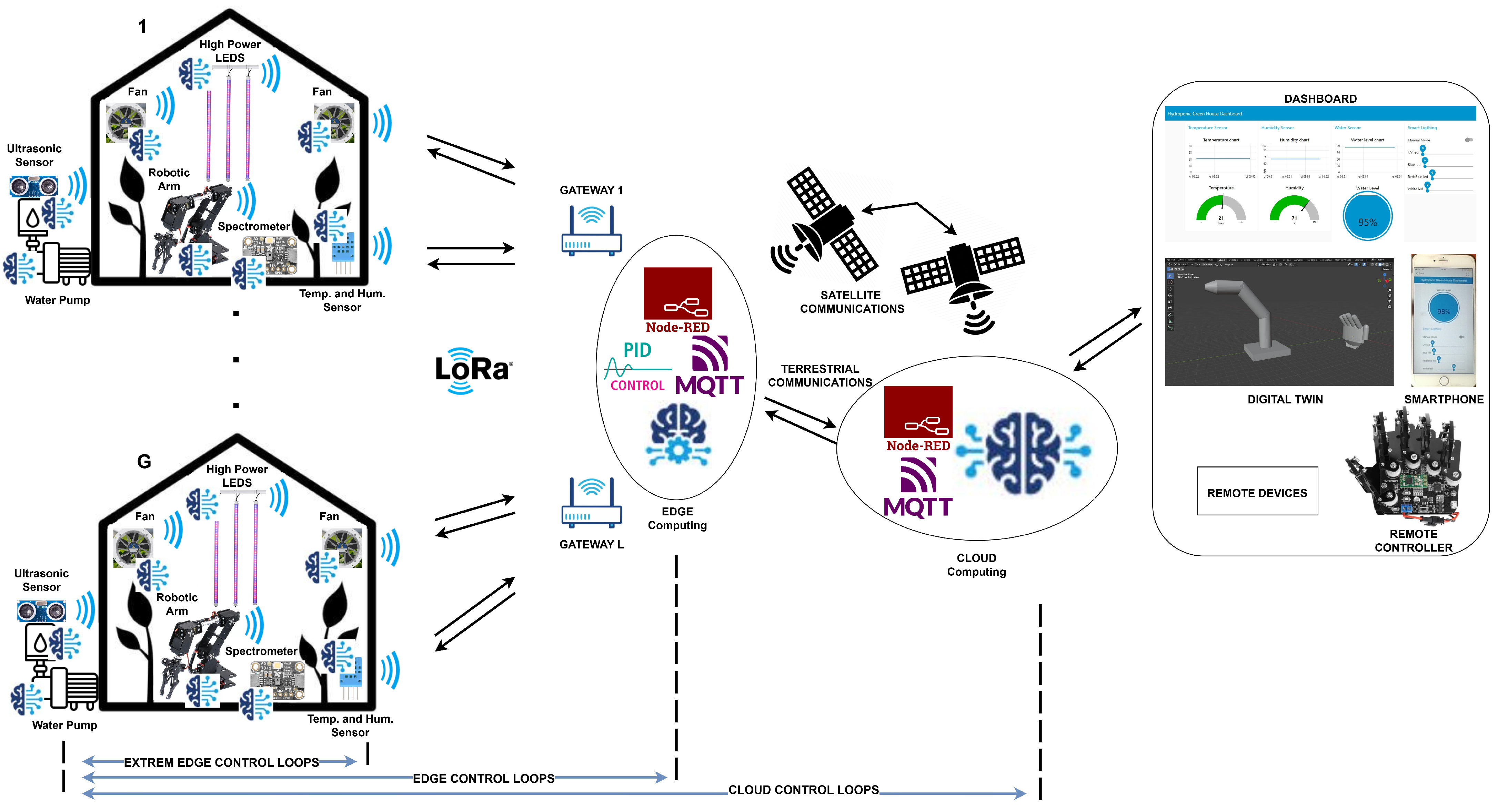
4.1. Network Architecture

The proposed network architecture comprises a certain number G of greenhouses, each containing a series of extreme edge devices for sensing and actuation. This component is represented on the left side of Figure 2, which illustrates the entire employed network architecture.

The extreme edge devices within the GHs communicate using LoRa modulation at 2.4 GHz, leveraging the capabilities of the latest SX1280 Semtech chip. Compared to other low-power consumption technologies such as ZigBee, SigFox, and IEEE 802.11ah (Wi-Fi HaLow) [37,38], LoRa offers several advantages: lower power consumption, greater robustness against interference, and a longer communication range of up to 10 km in line of sight [31,39]. This is particularly beneficial when GHs are installed in remote and/or rural areas far from the main building, where internet coverage is typically available. Moreover, employing LoRa at a 2.4 GHz frequency enables global compatibility and seamless usability without requiring special configurations or transmission authorization, unlike technologies operating in licensed spectrum.

For data processing and sharing, the concept of the cloud continuum is adopted, distributing computation across both the network edge and the centralized public cloud. Communication between these components occurs via the public internet, which is well known to utilize both terrestrial and satellite communications. This approach reduces communication latency for stringent actuation control loops by exploiting edge computing while simultaneously enabling more accurate decision-making and retrospective adjustment of prior decisions, due to the greater computational power offered by centralized cloud computing. The Node-RED low-code/no-code paradigm has been implemented both at the edge and in the cloud to facilitate the integration of new sensing and actuating devices into the GHs and to develop monitoring and control functions. The choice of using the computing server Node-RED is driven by its ability to facilitate data processing through an intuitive and fast block-based programming approach. As the transport protocol, Message Queuing Telemetry Transport (MQTT) has been employed among all entities in the network architecture: extreme edge devices, edge computing, cloud computing, and remote devices. This choice is justified by its simplicity of implementation and low processing overhead on the network [40].

The proposed network architecture also enables human interaction via remote devices, such as dashboards for visualizing monitored data like temperature and humidity trends, water trunk levels and light intensity, and issuing manual commands to be executed in the GHs, digital twins of specific GH services for monitoring their status and prototyping new functionalities, and wearable controllers for transmitting commands to the extreme edge devices [41].

In our application scenario, the developed network architecture consists of four distinct hydroponic greenhouses ($G=4$) and two gateways for LoRa coverage ($L=2$). Edge computing, incorporating the MQTT broker and Node-RED server, has been implemented on a Raspberry Pi 5 board, while cloud computing utilizes the public cloud Microsoft Azure. More specifically, the extreme edge devices installed in the GHs include [12] high-power LEDs (UV, red, blue, and white), temperature and humidity sensors, ultrasonic sensors, spectrometers, fans, robotic arms, and water pumps. Each of the aforementioned sensors and actuators is connected to the gateway and directly to others through an STM32 microcontroller and an SX1280 module.

Through this network architecture, three types of control loops can be developed: extreme edge control loops, edge control loops, and cloud control loops. Typically, in other architectures, only edge and cloud loops are utilized, transferring sensor data from the GH to external computing units. This enhances control accuracy and decision-making through more complex algorithms, benefiting from higher computational power. However, it also increases the latency between sensing and actuation (such as cooling system activation, water pump control and illumination adjustment). In case of stringent latency requirements, the optimal approach is to employ extreme edge control loops with direct communication between sensors and actuators. In this case, computing and decision-making must be performed immediately on the microcontroller, which is the primary focus of this paper. Indeed, our work reduces the complexity of the NNs in terms of memory-allocated variables and the number of FLOPs required for microclimate prediction and classification.

4.2. Dataset Construction

To demonstrate the validity and improvements of our approach, we installed a Davis Vantage PRO 2 weather station sensor [42] in each of the four GHs to collect temperature and humidity data with an accuracy of ±0.3 °C and ±2%, respectively. The four GHs contain cultivated tomato plants and are located in different areas of Pisa, Italy, which reduces the dependency between the collected data compared to having all GHs in the same location. Specifically, data were sampled every 15 min throughout the entirety of 2024, resulting in a dataset consisting of 35,136 samples per GH and monitored parameter, for a total of 281,088 recorded values.

In Figure 3, we illustrate the average temperature and humidity for the four distinct GHs (represented by different colors) across the four seasons.

From Figure 3, it can be observed that the mean temperature varies significantly across seasons compared to the variation in mean humidity. Moreover, among the different GHs, the temperature variation is more pronounced during summer and winter, whereas the variability in humidity remains more uniform across the GHs.

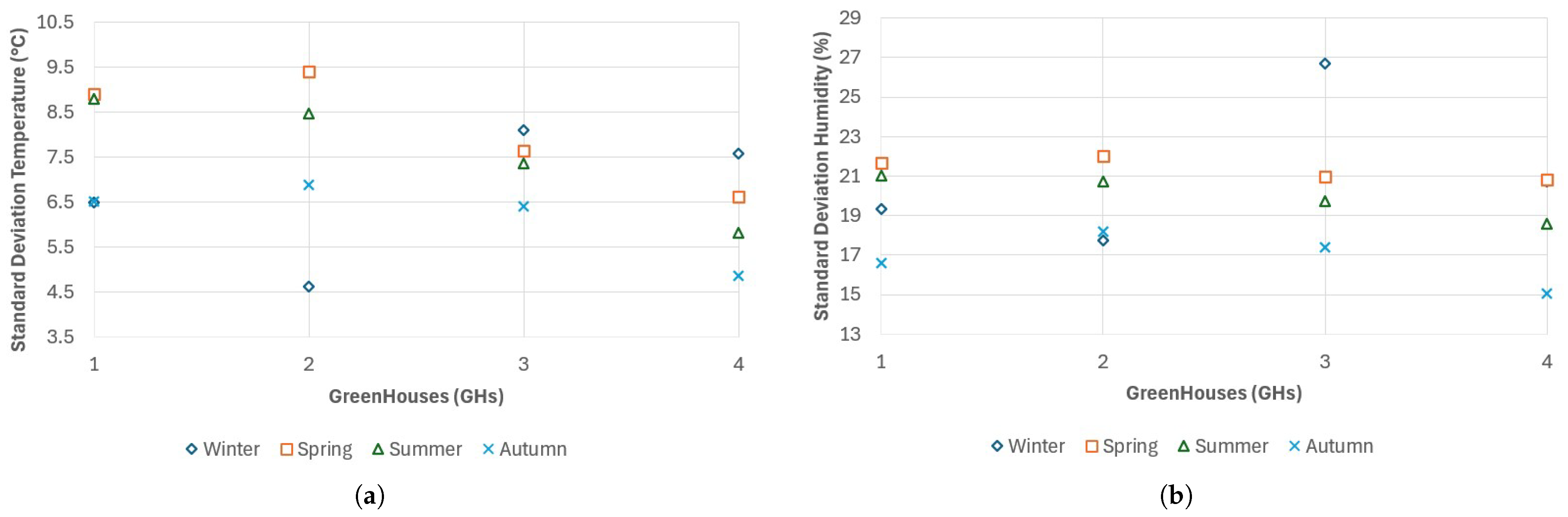
Conversely, Figure 4 shows the standard deviation of temperature and humidity across the GHs and throughout the seasons.

Regarding the standard deviation of temperature, it can be noted that the four GHs exhibit different behaviors. On the other hand, the humidity trend appears more uniform across the GHs, except for a peak during winter in GH3. Indeed, the fact that they are located in different areas reinforces the idea that the data from the various greenhouses are independent of one another.

Additionally,

Table 2. Maximum and minimum dataset values.

	Temp-GH1	Hum-GH1	Temp-GH2	Hum-GH2	Temp-GH3	Hum-GH3	Temp-GH4	Hum-GH4	Global-Temp	Global-Hum
Min	1.16	9.84	−4.04	12.25	−2.55	15.18	−1.26	11.70	−4.04	9.84
Max	53.43	93.67	52.58	99.07	47.78	98.49	46.21	99.15	53.43	99.15

presents the minimum and maximum temperature and humidity values for each GH, as well as the global values for the dataset, which are later utilized in Section 4.3.

4.3. Hybrid Neural Network and Fuzzy Proposed Approach

Our hybrid approach incorporates a NN for time series prediction, followed by a fuzzy layer to classify the NN’s output; specifically, greenhouse microclimate conditions. The primary objective is to reduce NN complexity while maintaining performance levels in a way that is comparable to those of a standard NN classifier. In particular, we have chosen a FFNN as our reference NN model, as explained in Section 3.

The FFNN consists of an input layer, a hidden layer, and an output layer. The input layer receives past temperature and humidity values at hourly intervals. During the search for the optimal configuration, the number of input features will be varied, as discussed in Section 5. Additionally, the size of the hidden layer, defined by the number of interconnected nodes between the input and output layers, will be adjusted in the experimental trials. Finally, the output layer generates two numerical outputs, corresponding to the predicted temperature and humidity for the next hour. These predicted values will then be processed by the fuzzy layer to produce the final microclimate classification.

Our proposed solution is compared to the standard approach, in which the NN directly outputs the final microclimate classification.

For training both the proposed and standard NN models, we employed the Levenberg–Marquardt algorithm [34], which is commonly used for this purpose.

Regarding the activation function, our approach utilizes the ReLU function, as it provides the numerical temperature and humidity predictions required for the fuzzy layer. In contrast, the standard approach employs the sigmoid function, which outputs probabilities for microclimate classification.

For backpropagation, both approaches use MSE to compute the gradient of the loss function with respect to the selected weights and biases.

More specifically, our approach integrates numerical predictions from the FFNN with the concept of granular computing, in particular fuzzy sets, aiming not only to reduce the complexity and size of the NN architecture but also to enhance the interpretability and reliability of the predicted classifications.

Fuzzy sets are defined as follows [43]:

Definition 1. 

Given a domain $\mathcal{X}$, with x being a generic element of $\mathcal{X}$, the fuzzy set A in $\mathcal{X}$ is defined as the set of pairs $A=(x,f_A\left(x\right))$, characterized by a membership function $f_A\left(x\right)$ that associates a real number in the interval $[0,1]$ with each element of $\mathcal{X}$. The value of $f_A\left(x\right)$ represents the degree of membership of x in A.

• For $f_A\left(x\right)=1$, x definitely belongs to A.
• For $f_A\left(x\right)=0$, x does not belong to A.
• For $0<f_A\left(x\right)<1$, x partially belongs to A.

For the fuzzy sets, we employed triangular membership functions, as they provide a more accurate representation of phenomena exhibiting gradual and continuous variations. The triangular membership function is defined as follows:

$$f_A(x;a,b,c)=max\left(min\left({\displaystyle \frac{x-a}{b-a}},{\displaystyle \frac{c-x}{c-b}}\right),0\right),$$

(5)

where a and c define the base points of the triangle, while b represents the peak position.

With reference to tomato plant cultivation, we set the optimal growth thresholds for temperature and humidity according to

Table 3. Fuzzy sets thresholds.

Level	Temperature (°C)	Humidity (%)
Low	[$m_t$, 16, 19]	[$m_h$, 35, 45]
Optimal	[18, 24, 30]	[40, 55, 70]
High	[29, 32, $M_t$]	[65, 73, $M_h$]

, based on [44].

Each cell follows the format [a, b, c], as in Equation (5). Additionally, $m_t$ and $m_h$ represent the global minimum temperature and humidity values in the dataset, while $M_t$ and $M_h$ denote their respective global maximum values, as shown in Table 2. In this way, each temperature and humidity value will be associated with a fuzzy set through a specific degree of membership for each membership function, ranging from zero to one. The membership functions constructed in this manner take into account all input values from the dataset, from the minimum to the maximum.

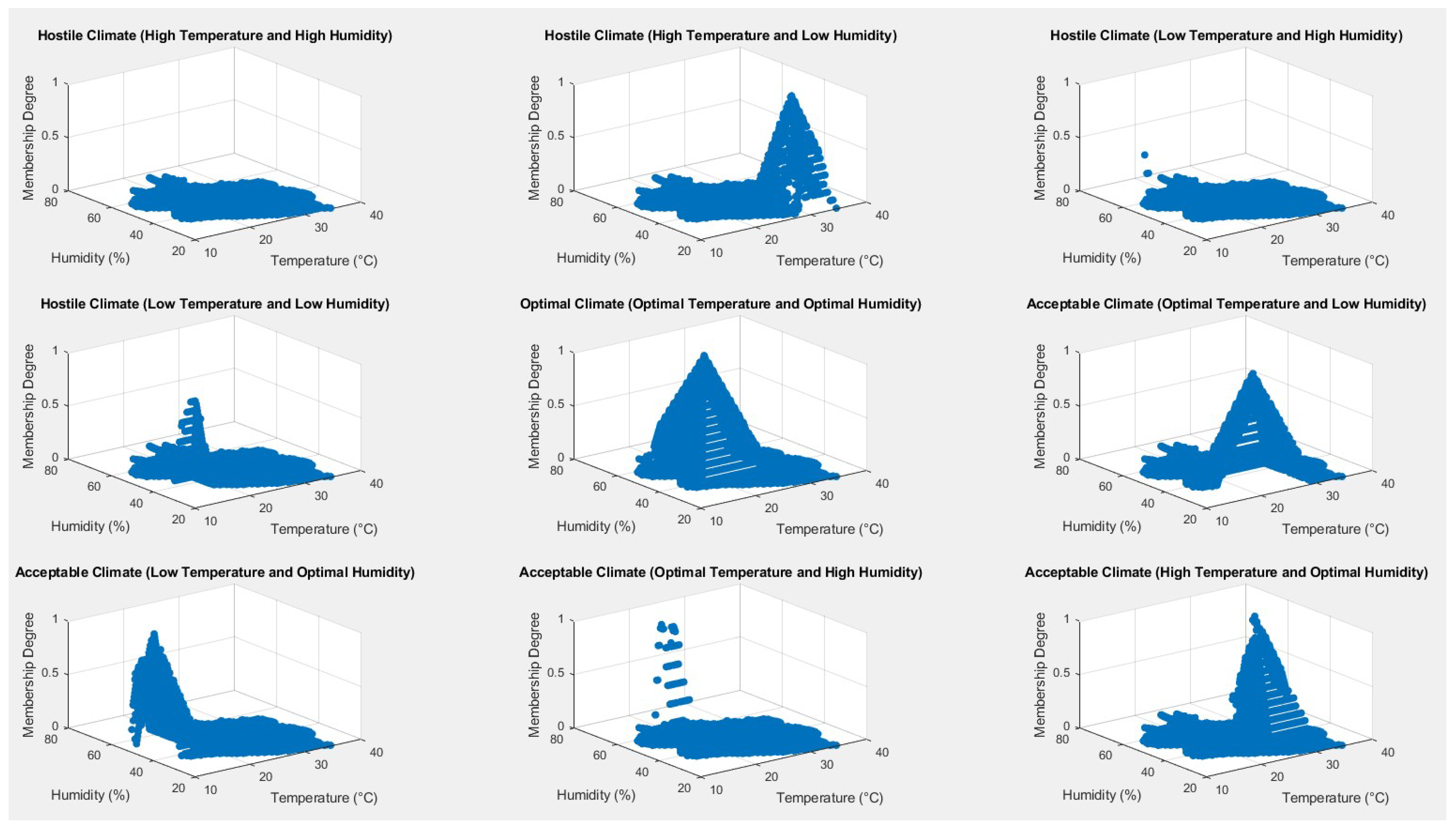
To resume, the fuzzy layer consists of six triangular membership functions, each corresponding to a different class of temperature and humidity: low temperature, optimal temperature, high temperature, low humidity, optimal humidity, and high humidity.

Using these six membership functions, we defined the final microclimate classifications based on a rule set that combines temperature and humidity membership functions. This rule set uses the values of the membership functions to determine their influence on the final classification. Specifically, the final classification is computed by finding the minimum of the membership degrees for each combination of temperature and humidity membership functions, resulting in nine decision classification degrees, corresponding to the entries of

Table 4. Climate decision classification.

		Temperature
		Low	Optimal	High	Outlier
Humidity	Low	Hostile	Acceptable	Hostile	OOK
	Optimal	Acceptable	Optimal	Acceptable	OOK
	High	Hostile	Acceptable	Hostile	OOK
	Outlier	OOK	OOK	OOK	OOK

, excluding Out of Knowledge (OOK). Among the nine decision classification degrees, the maximum is identified and selected as the final classification. If the maximum is zero, the system will return the OOK classification. As detailed in Table 4, the possible final classifications are Optimal, Acceptable, Hostile microclimate conditions, and OOK prediction.

An additional advantage of the proposed approach is the ability to output an OOK classification, enhancing the reliability of classifications derived from the FFNN’s numerical predictions. It is well known that NNs always generate an output, even in cases where the prediction is unreliable. To mitigate this issue, our approach introduces a dedicated OOK classification when the predicted temperature and/or humidity values do not fall within any of the previously defined triangular fuzzy sets. This prevents the generation of misleading outputs outside the reliability ranges, i.e., the range of values present in the dataset used for training, from which the NN learned the temporal patterns.

Finally, to evaluate the overall performance of the proposed approach (FFNN + fuzzy) and the standard approach, we employed the $F_{1}score$ metric, defined by the following Equation (6):

$$F_{1}score={\displaystyle \frac{2TP}{2TP+FP+FN}},$$

(6)

where $TP=\#TruePositive$, $FP=\#FalsePositive$, and $FN=\#FalseNegative$.

5. Results

In this section, we present and discuss the experimental results obtained by applying the methodology described in Section 4.

Firstly, in order to provide a descriptive overview of the dataset’s characteristics with respect to microclimate classification, in Figure 5, we show the membership function values for the various climate classes. In particular, in accordance with Table 4, we display the membership functions (on the z-axis) for the nine climate combinations, as specified by the rule list, in 3D graphs with temperature and humidity values along the horizontal $xy$ axes that are then mapped and merged into the final microclimate classifications. It is worth noting that, considering the entire dataset, the OOK classification is excluded from this representation as it was obviously never observed here.

Furthermore, as can be seen in Figure 5, some cases of hostile climate classification appear rarely in our dataset, with membership degree values reportedly close to zero. This occurs, for example, in the following situations: high temperature–high humidity, low–high, and low–low.

Regarding the training phase of the FFNN for both the standard and proposed approaches, we utilized temperature and humidity data from three GHs, while the other one was employed for the validation phase, during which the experimental performance was measured. To ensure a more accurate evaluation, we repeated this methodology 20 times, swapping the combinations of GHs used for training and validation. In each of these trials, we computed a global $F_{1}score$ by averaging the $F_{1}score$ of each microclimate class described previously, and finally, we averaged this parameter across all the trials. These results are reported in

Table 5. $F_{1}score$ with standard FFNN approach.

${\mathit{n}}_{\mathit{i}}$/${\mathit{n}}_{\mathit{h},1}$	10	20	30	50	60	80	100	120
10	04844	0.6144	0.6100	0.6557	0.6172	0.6237	0.6200	0.5911
8	0.5316	0.5390	0.5448	0.6027	0.6098	0.6344	0.6041	0.6336
6	0.4894	0.4541	0.5660	0.5818	0.5355	0.5517	0.5835	0.5949
4	0.4747	0.5886	0.5316	0.5088	0.4949	0.5503	0.4985	0.5644
2	0.4870	0.4384	0.5486	0.5756	0.4905	0.5220	0.5116	0.5561
$n_i$/$n_{h,1}$	150	160	170	180	190	200	250	300
10	0.6184	0.6363	0.5966	0.6386	0.6438	0.6200	0.6109	0.6034
8	0.6171	0.5971	0.5739	0.6169	0.5963	0.6486	0.5794	0.6107
6	0.5470	0.6133	0.5731	0.5985	0.5292	0.5520	0.5842	0.6012
4	0.5136	0.6012	0.5057	0.5523	0.4966	0.4988	0.5090	0.5096
2	0.5202	0.5314	0.4943	0.5865	0.6011	0.5218	0.5605	0.5503

and

Table 6. $F_{1}score$ with proposed fuzzy-based FFNN approach.

${\mathit{n}}_{\mathit{i}}$/${\mathit{n}}_{\mathit{h},1}$	3	4	6	8	10	20	30	50	60	80
10	0.6418	0.6627	0.6819	0.6752	0.6896	0.6927	0.6927	0.6836	0.6933 *	0.6925
8	0.6353	0.6256	0.6649	0.6697	0.6675	0.6786	0.6841	0.6782	0.6728	0.6772
6	0.5979	0.6085	0.6192	0.6595	0.6550	0.6558	0.6619	0.6675	0.6573	0.6624
4	0.6110	0.6194	0.6288	0.6318	0.6405	0.6410	0.6438	0.6446	0.6425	0.6425
2	0.5520	0.5600	0.5607	0.5594	0.5579	0.5619	0.5652	0.5632	0.5599	0.5637
$n_i$/$n_{h,1}$	100	120	150	160	170	180	190	200	250	300
10	0.6711	0.6828	0.6727	0.6762	0.6751	0.6692	0.6725	0.6699	0.6742	0.6544
8	0.6735	0.6716	0.6726	0.6752	0.6738	0.6756	0.6721	0.6637	0.6632	0.6660
6	0.6729	0.6668	0.6618	0.6586	0.6491	0.6597	0.6485	0.6534	0.6489	0.6392
4	0.6352	0.6450	0.6414	0.6347	0.6455	0.6378	0.6361	0.6458	0.6248	0.6322
2	0.5638	0.5623	0.5570	0.5590	0.5550	0.5606	0.5560	0.5583	0.5493	0.5526

for the standard approach and the proposed fuzzy-based approach, respectively.

For the identification of the optimal FFNN model and the subsequent comparison with the proposed fuzzy-based approach, we considered as input the past hourly values of temperature and humidity grouped into sets of 10, 8, 6, 4, and 2. Specifically, each group was equally divided between past temperature and humidity values, based on the high correlation observed between these past measurements and the target prediction. Simultaneously, we tested various configurations for the number of nodes in the fixed hidden layer ($n_{h,1}$). The maximum tested value of 300 nodes for the hidden layer represents a compromise between overfitting and model accuracy. In fact, as shown in Table 5, the $F_{1}score$, after a number of hidden layer nodes greater than or equal to 190, appears to exhibit a decreasing trend.

With the standard approach, we would choose the configuration that produces the highest $F_{1}score$ among those tested, namely $n_i$ equal to 10 and $n_{h,1}$ equal to 50, as highlighted in bold in Table 5. Conversely, following the proposed fuzzy-based approach, to maintain an equitable level of accuracy and to compare the difference in complexity, we choose the architecture with an $F_{1}score$ greater than or equal to that of the standard approach, achieved with minimal architectural complexity. Specifically, with this approach, we select $n_i$ equal to 10 and $n_{h,1}$ equal to 4, as highlighted in bold in Table 6. It is worth noting that the reported $F_{1}score$ results include the OOK classification. In fact, the values of the validation dataset that are near the extremes of the fuzzy sets of temperature and humidity, and thus have a very low membership degree, lead to outlier predictions and, consequently, to the OOK classification.

In Figure 6, the comparison between the number of variables allocated in memory (a) and the number of FLOPs (b) is shown for both the FFNN with the standard approach and the proposed fuzzy-based approach.

Specifically, with the proposed approach, the following reductions in the architectural complexity of the FFNN component are achieved:

• The number of variables allocated in memory is reduced by 92.32%;
• The number of Floating Point Operations is reduced by 94.26%.

These improvements facilitate the deployment of the FFNN on hardware with limited computational capabilities, particularly at the extreme edge of the network.

Conversely, when NNs are deployed at the edge, the primary objective shifts toward maximizing classification accuracy and prediction performance, without the strict constraints of computational limitations. In such scenarios, the proposed fuzzy-based approach achieves superior performance, reaching higher classification accuracy with the globally optimal architecture consisting of 10 inputs and 60 hidden nodes, as highlighted in italics and marked with an asterisk in Table 6. In this configuration, the method achieves a 6% improvement in performance.

However, the proposed methodology and the work conducted also have some limitations. First, the technique should be further evaluated on other types of NNs to determine whether its effectiveness extends beyond feed-forward architectures. Another limitation concerns the applicability of the approach itself: it is not a general-purpose method that guarantees improvements when applied to NNs. Instead, it is particularly well suited to scenarios involving time-series numerical data used for classification and prediction tasks.

Nonetheless, an additional advantage of the proposed fuzzy-based approach lies in its flexibility. It enables the rapid adaptation of the model to different crops that require customized microclimate thresholds. In practice, the same trained FFNN can be reused by simply updating the fuzzy sets in the fuzzy layer to reflect new classification criteria. This stands in contrast to the conventional approach, which would require retraining the FFNN and redefining the final classification labels within the dataset.

6. Conclusions

This work aims to introduce a novel approach to time series classification in order to reduce the computational complexity of the employed NN. More specifically, we have considered the classification and prediction of the microclimate within greenhouses as an application scenario. For monitoring and executing control commands, we have also proposed a network architecture to enable the execution of predictive algorithms in different zones. In this context, we collected temperature and humidity data from four real greenhouses. By integrating the concepts of NNs and granular computing, we employed an FFNN to predict the point values of the microclimate and then render the information granular through fuzzy sets for the final classification.

With the introduced approach, we increased the credibility and reliability of the predictions by incorporating Out-of-knowledge classification when the predicted data fell outside the training intervals of the NN. Compared to the standard approach, which uses the FFNN directly as a classifier, the proposed approach is able to guarantee the same prediction accuracy ($F_{1}score$) while significantly reducing the complexity of the underlying model. More specifically, it reduces the number of variables allocated in the memory by approximately 92% and the number of FLOPs by 94%. This enables implementation on boards located at the extreme edge of the network, where computational and energy constraints are critical, reducing both inference time and energy consumption while maintaining the same model accuracy. As a result, certain decisions can be made directly in the field, thereby reducing the latency associated with responses from edge or cloud computing systems.

References

1. Qazi, S.; Khawaja, B.A.; Farooq, Q.U. IoT-Equipped and AI-Enabled Next Generation Smart Agriculture: A Critical Review, Current Challenges and Future Trends. IEEE Access 2022, 10, 21219–21235. [Google Scholar] [CrossRef]
2. Rayhana, R.; Xiao, G.; Liu, Z. Internet of Things Empowered Smart Greenhouse Farming. IEEE J. Radio Freq. Identif. 2020, 4, 195–211. [Google Scholar] [CrossRef]
3. Ünal, Z. Smart Farming Becomes Even Smarter with Deep Learning—A Bibliographical Analysis. IEEE Access 2020, 8, 105587–105609. [Google Scholar] [CrossRef]
4. Chen, X.; Chen, W.; Dinavahi, V.; Liu, Y.; Feng, J. Short-Term Load Forecasting and Associated Weather Variables Prediction Using ResNet-LSTM Based Deep Learning. IEEE Access 2023, 11, 5393–5405. [Google Scholar] [CrossRef]
5. Yang, Y.; Gao, P.; Sun, Z.; Wang, H.; Lu, M.; Liu, Y.; Hu, J. Multistep ahead prediction of temperature and humidity in solar greenhouse based on FAM-LSTM model. Comput. Electron. Agric. 2023, 213, 108261. [Google Scholar] [CrossRef]
6. Liu, Y.; Li, D.; Wan, S.; Wang, F.; Dou, W.; Xu, X.; Li, S.; Ma, R.; Qi, L. A long short-term memory-based model for greenhouse climate prediction. Int. J. Intell. Syst. 2022, 37, 135–151. [Google Scholar] [CrossRef]
7. Kalyani, Y.; Collier, R. A Systematic Survey on the Role of Cloud, Fog, and Edge Computing Combination in Smart Agriculture. Sensors 2021, 21, 5922. [Google Scholar] [CrossRef]
8. Zaidi, S.A.R.; Hayajneh, A.M.; Hafeez, M.; Ahmed, Q.Z. Unlocking Edge Intelligence Through Tiny Machine Learning (TinyML). IEEE Access 2022, 10, 100867–100877. [Google Scholar] [CrossRef]
9. Falanji, R.; Heusse, M.; Duda, A. Range and capacity of lora 2.4 ghz. In Proceedings of the International Conference on Mobile and Ubiquitous Systems: Computing, Networking, and Services; Springer: Berlin/Heidelberg, Germany, 2022; pp. 403–421. [Google Scholar]
10. Bembe, M.; Abu-Mahfouz, A.; Masonta, M.; Ngqondi, T. A survey on low-power wide area networks for IoT applications. Telecommun. Syst. 2019, 71, 249–274. [Google Scholar] [CrossRef]
11. Mukherji, A.; Sadu, S. ZigBee performance analysis. In Proceedings of the 2016 International Conference on Wireless Communications, Signal Processing and Networking (WiSPNET), Chennai, India, 23–25 March 2016; pp. 325–329. [Google Scholar]
12. Bua, C.; Adami, D.; Giordano, S. GymHydro: An Innovative Modular Small-Scale Smart Agriculture System for Hydroponic Greenhouses. Electronics 2024, 13, 1366. [Google Scholar] [CrossRef]
13. Chen, H.Y.; Sharma, K.; Sharma, C.; Sharma, S. Integrating explainable artificial intelligence and blockchain to smart agriculture: Research prospects for decision making and improved security. Smart Agric. Technol. 2023, 6, 100350. [Google Scholar] [CrossRef]
14. Gunning, D.; Stefik, M.; Choi, J.; Miller, T.; Stumpf, S.; Yang, G.Z. XAI—Explainable artificial intelligence. Sci. Robot. 2019, 4, eaay7120. [Google Scholar] [CrossRef] [PubMed]
15. Hoshino, Y.; Rathnayake, N.; Dang, T.L.; Rathnayake, U. Cascaded-ANFIS and Its Successful Real-World Applications. In Fuzzy Logic Controllers and Applications; Balasubramaniam, P., Babu, N.R., Eds.; IntechOpen: Rijeka, Croatia, 2024; Chapter 3. [Google Scholar] [CrossRef]
16. Rathnayake, N.; Miyazaki, A.; Dang, T.L.; Hoshino, Y. Age Classification of Rice Seeds in Japan Using Gradient-Boosting and ANFIS Algorithms. Sensors 2023, 23, 2828. [Google Scholar] [CrossRef] [PubMed]
17. He, Y.; Zhang, X.; Sun, J. Channel Pruning for Accelerating Very Deep Neural Networks. In Proceedings of the 2017 IEEE International Conference on Computer Vision (ICCV), Venice, Italy, 22–29 October 2017; pp. 1398–1406. [Google Scholar] [CrossRef]
18. Yan, M.; Zhao, M.; Xu, Z.; Zhang, Q.; Wang, G.; Su, Z. VarGFaceNet: An Efficient Variable Group Convolutional Neural Network for Lightweight Face Recognition. In Proceedings of the 2019 IEEE/CVF International Conference on Computer Vision Workshop (ICCVW), Seoul, Republic of Korea, 27–28 October 2019. [Google Scholar]
19. Chen, S.; Lin, L.; Zhang, Z.; Gen, M. Evolutionary NetArchitecture Search for Deep Neural Networks Pruning. In Proceedings of the 2019 2nd International Conference on Algorithms, Computing and Artificial Intelligence, ACAI ’19, New York, NY, USA, 20–22 December 2019; pp. 189–196. [Google Scholar] [CrossRef]
20. Yao, S.; Zhao, Y.; Zhang, A.; Su, L.; Abdelzaher, T. DeepIoT: Compressing Deep Neural Network Structures for Sensing Systems with a Compressor-Critic Framework. In Proceedings of the 15th ACM Conference on Embedded Network Sensor Systems, New York, NY, USA, 5–7 November 2017. SenSys ’17. [Google Scholar] [CrossRef]
21. Parashar, A.; Rhu, M.; Mukkara, A.; Puglielli, A.; Venkatesan, R.; Khailany, B.; Emer, J.; Keckler, S.W.; Dally, W.J. SCNN: An Accelerator for Compressed-Sparse Convolutional Neural Networks. arXiv 2017, arXiv:1708.04485. [Google Scholar]
22. Chauhan, J.; Rajasegaran, J.; Seneviratne, S.; Misra, A.; Seneviratne, A.; Lee, Y. Performance Characterization of Deep Learning Models for Breathing-Based Authentication on Resource-Constrained Devices. Proc. ACM Interact. Mob. Wearable Ubiquitous Technol. 2018, 2, 1–24. [Google Scholar] [CrossRef]
23. Han, S.; Mao, H.; Dally, W.J. Deep Compression: Compressing Deep Neural Networks with Pruning, Trained Quantization and Huffman Coding. arXiv 2016, arXiv:1510.00149. [Google Scholar]
24. Jacob, B.; Kligys, S.; Chen, B.; Zhu, M.; Tang, M.; Howard, A.; Adam, H.; Kalenichenko, D. Quantization and Training of Neural Networks for Efficient Integer-Arithmetic-Only Inference. arXiv 2017, arXiv:1712.05877. [Google Scholar]
25. Contoli, C.; Lattanzi, E. A Study on the Application of TensorFlow Compression Techniques to Human Activity Recognition. IEEE Access 2023, 11, 48046–48058. [Google Scholar] [CrossRef]
26. Umuroglu, Y.; Fraser, N.J.; Gambardella, G.; Blott, M.; Leong, P.; Jahre, M.; Vissers, K. FINN: A Framework for Fast, Scalable Binarized Neural Network Inference. In Proceedings of the 2017 ACM/SIGDA International Symposium on Field-Programmable Gate Arrays, FPGA ’17, New York, NY, USA, 22–24 February 2017; pp. 65–74. [Google Scholar] [CrossRef]
27. Eshratifar, A.E.; Pedram, M. Runtime Deep Model Multiplexing for Reduced Latency and Energy Consumption Inference. In Proceedings of the 2020 IEEE 38th International Conference on Computer Design (ICCD), Hartford, CT, USA, 18–21 October 2020; pp. 263–270. [Google Scholar] [CrossRef]
28. Georgiev, P.; Bhattacharya, S.; Lane, N.D.; Mascolo, C. Low-resource Multi-task Audio Sensing for Mobile and Embedded Devices via Shared Deep Neural Network Representations. Proc. ACM Interact. Mob. Wearable Ubiquitous Technol. 2017, 1, 50. [Google Scholar] [CrossRef]
29. Abbasi, S.; Hajabdollahi, M.; Karimi, N.; Samavi, S. Modeling Teacher-Student Techniques in Deep Neural Networks for Knowledge Distillation. arXiv 2019, arXiv:1912.13179. [Google Scholar]
30. Hinton, G.; Vinyals, O.; Dean, J. Distilling the Knowledge in a Neural Network. arXiv 2015, arXiv:1503.02531. [Google Scholar]
31. Mishra, R.; Gupta, H.P.; Dutta, T. A Survey on Deep Neural Network Compression: Challenges, Overview, and Solutions. arXiv 2020, arXiv:2010.03954. [Google Scholar]
32. Bua, C.; Fiorini, F.; Adami, D.; Giordano, S.; Pagano, M. Enhancing Climate Prediction in Smart Greenhouse: Synergy of Neural Network and Granular Computing to Reduce Computational Complexity. In Proceedings of the 2024 IEEE International Workshop on Metrology for Agriculture and Forestry (MetroAgriFor), Padua, Italy, 29–31 October 2024; pp. 226–231. [Google Scholar] [CrossRef]
33. Ma, X.; Yao, T.; Hu, M.; Dong, Y.; Liu, W.; Wang, F.; Liu, J. A Survey on Deep Learning Empowered IoT Applications. IEEE Access 2019, 7, 181721–181732. [Google Scholar] [CrossRef]
34. Levenberg, K. A method for the solution of certain non—Linear problems in least squares. Q. Appl. Math. 1944, 2, 164–168. [Google Scholar] [CrossRef]
35. Apicella, A.; Donnarumma, F.; Isgrò, F.; Prevete, R. A survey on modern trainable activation functions. Neural Netw. 2021, 138, 14–32. [Google Scholar] [CrossRef]
36. Dubey, S.R.; Singh, S.K.; Chaudhuri, B.B. Activation functions in deep learning: A comprehensive survey and benchmark. Neurocomputing 2022, 503, 92–108. [Google Scholar] [CrossRef]
37. Liu, Z.; Li, Y.; Zhao, L.; Liang, R.; Wang, P. Comparative Evaluation of the Performance of ZigBee and LoRa Wireless Networks in Building Environment. Electronics 2022, 11, 3560. [Google Scholar] [CrossRef]
38. Polak, L.; Milos, J. Performance analysis of LoRa in the 2.4 GHz ISM band: Coexistence issues with Wi-Fi. Telecommun. Syst. 2020, 74, 299–309. [Google Scholar] [CrossRef]
39. Falanji, R.; Heusse, M.; Duda, A. Range and Capacity of LoRa 2.4 GHz. In Mobile and Ubiquitous Systems, Proceedings of the Computing, Networking and Services, Melbourne, VIC, Australia, 14–17 November 2023; Longfei, S., Bodhi, P., Eds.; Springer Nature: Cham, Switzerland, 2023; pp. 403–421. [Google Scholar]
40. Lakshminarayana, S.; Praseed, A.; Thilagam, P.S. Securing the IoT Application Layer from an MQTT Protocol Perspective: Challenges and Research Prospects. IEEE Commun. Surv. Tutor. 2024, 26, 2510–2546. [Google Scholar] [CrossRef]
41. Bua, C.; Borgianni, L.; Adami, D.; Giordano, S. Empowering Remote Agriculture: Wearable Glove Control for Smart Hydroponic Greenhouses. In Proceedings of the 2024 IEEE 25th International Conference on High Performance Switching and Routing (HPSR), Pisa, Italy, 22–24 July 2024; pp. 215–220. [Google Scholar] [CrossRef]
42. Vantage PRO 2 Weather Station Specifications. Available online: https://www.meteoproject.it/davis-vantage-pro2.php (accessed on 11 November 2024).
43. Pedrycz, W. An Introduction to Computing with Fuzzy Sets; Intelligent Systems Reference Library; Springer: Cham, Switzerland, 2020. [Google Scholar] [CrossRef]
44. Shamshiri, R.R.; Jones, J.W.; Thorp, K.R.; Ahmad, D.; Man, H.C.; Taheri, S. Review of optimum temperature, humidity, and vapour pressure deficit for microclimate evaluation and control in greenhouse cultivation of tomato: A review. Int. Agrophysics 2018, 32, 287–302. [Google Scholar] [CrossRef]
Figure 1. FFNN-node computations.
Futureinternet 17 00214 g001
Figure 2. Network architecture.
Futureinternet 17 00214 g002
Figure 3. Average temperature (a) and humidity (b) values for different greenhouses and seasons.
Futureinternet 17 00214 g003
Figure 4. Standard deviation of temperature (a) and humidity (b) values for different greenhouses and seasons.
Futureinternet 17 00214 g004
Figure 5. Climate membership degree classification.
Futureinternet 17 00214 g005
Figure 6. Number of variables (a) and FLOPs (b) with the standard FFNN approach and proposed fuzzy-based approach.
Futureinternet 17 00214 g006