Article

A Resilient Deep Learning Framework for Mobile Malware Detection: From Architecture to Deployment

1
College of Information Technology, University of Bahrain, Sakhir P.O. Box 32038, Bahrain
2
College of Computing, Umm Al-Qura University (UQU), Makkah 21955, Saudi Arabia
*
Author to whom correspondence should be addressed.
Future Internet 2025, 17(12), 532; https://doi.org/10.3390/fi17120532
Submission received: 16 October 2025 / Revised: 15 November 2025 / Accepted: 19 November 2025 / Published: 21 November 2025
(This article belongs to the Special Issue Cybersecurity in the Age of AI, IoT, and Edge Computing)

Abstract

Mobile devices are frequent targets of malware due to the large volume of sensitive personal, financial, and corporate data they process. Traditional static, dynamic, and hybrid analysis methods are increasingly insufficient against evolving threats. This paper proposes a resilient deep learning framework for Android malware detection, integrating multiple models and a CPU-aware selection algorithm to balance accuracy and efficiency on mobile devices. Two benchmark datasets (i.e., the Android Malware Dataset for Machine Learning and CIC-InvesAndMal2019) were used to evaluate five deep learning models: DNN, CNN, RNN, LSTM, and CNN-LSTM. The results show that CNN-LSTM achieves the highest detection accuracy of 97.4% on CIC-InvesAndMal2019, while CNN delivers strong accuracy of 98.07%, with the lowest CPU usage (5.2%) on the Android Dataset, making it the most practical for on-device deployment. The framework is implemented as an Android application using TensorFlow Lite, providing near-real-time malware detection with an inference time of under 150 ms and memory usage below 50 MB. These findings confirm the effectiveness of deep learning for mobile malware detection and demonstrate the feasibility of deploying resilient detection systems on resource-constrained devices.

1. Introduction

The increasing number of mobile devices has led to a rise in mobile malware. For example, the Android Play Store hosts more than 3.9 million apps [1]. This proliferation leaves devices vulnerable to cyberattacks [2]. Various malware detection methods exist as defense mechanisms, but their effectiveness depends on the factors they address. Android malware has become a serious problem, requiring effective countermeasures. Studies show that traditional static, dynamic, and hybrid analysis methods remain vulnerable. As malware grows more sophisticated, deep learning models have proven more effective in identifying it [3].
IoCs and machine learning are important tools in modern cybersecurity. IoCs provide critical information for incident response, malware detection, and heuristic analysis. Machine learning enhances detection by classifying malware based on patterns and features in the data [4].
However, malware detection for mobile devices faces several challenges:
  • Diverse Security Threats: Mobile devices are vulnerable to theft, social engineering, and loss, all of which can expose sensitive data.
  • Growing Data Sensitivity: Mobile devices store increasing amounts of personal, financial, and business data, making them prime targets.
  • Evolving Malware Landscape: Attackers constantly develop new methods to bypass defenses [5].
  • Real-Time Protection Needs: Always-connected devices require real-time protection. Traditional solutions often fall short [6]. The real-time constraints depend heavily on the device’s interactive latency and characteristics.
This study aims to build a deep learning–based malware classification system that adjusts its inference process according to the CPU capacity of Android devices. The work introduces a novel integration of model accuracy optimization and real-time or near-real-time resource awareness, making it practical for use on devices with limited hardware.
The research contributes to the literature in three main ways:
  • It introduces a CPU-adaptive multi-model design that dynamically selects the most suitable neural network at runtime depending on system load.
  • It conducts a structured evaluation of five deep learning architectures (DNN, CNN, RNN, LSTM, CNN-LSTM) across two preprocessing settings to explore the balance between dimensionality reduction and performance.
  • It demonstrates a working prototype, implemented as a TensorFlow Lite Android app, confirming the framework’s robustness and scalability in real-world use.
Instead of proposing a new detection algorithm, this study introduces a unified management process that coordinates model selection according to device workload, supported by a structured benchmarking pipeline and validated through real-world deployment. This integration of deep learning models into a CPU-adaptive control framework marks a new step in connecting offline malware detection research with practical on-device enforcement.
The remainder of this paper is structured as follows. Section 2 reviews the foundations of mobile malware detection, including Indicators of Compromise (IoCs), traditional detection techniques, and recent machine and deep learning approaches. Section 3 presents the proposed resilient deep learning framework, detailing the architecture, preprocessing pipeline, and model selection strategy. Section 4 describes the experimental setup, including datasets, training scenarios, and preprocessing steps. Section 5 reports the evaluation outcomes across two benchmark datasets and compares the performance of different deep learning models. Section 6 discusses the deployment of the optimized models on an Android application, highlighting functional testing and on-device performance. Section 7 provides a critical discussion of the results, comparing them with related work and outlining strengths and limitations. Finally, Section 8 concludes the paper and suggests future research directions.

2. Background and Related Work

Improving mobile device security and overcoming obstacles in mobile virus detection are significant applications of artificial intelligence (AI). Among AI approaches, machine learning (ML) is particularly effective for mobile malware detection and prevention, especially on Android systems [7]. A significant challenge in creating effective malware detection systems is the acquisition of labeled and current data to refresh detection models [8]. Many existing methods of mobile malware detection can be used as protective measures. Thus, the methods’ respective capabilities vary according to the factors upon which they concentrate [9]. This research presents the categories of mobile malware, associated threats, and existing detection solutions.

2.1. Indicators of Compromise (IoCs)

Indicators of Compromise (IOC) are forensic hints of a potential breach within a network or system. IOCs provide security teams with context for identifying and stopping cyberattacks early [10]. They include IP addresses, virus signatures, URLs, and domain names of botnets. The rapid development of threats generates IOC data at high speed, making collection and management challenging [11]. Security teams evaluate detected IOCs for threats and verify their authenticity. IOCs also reveal what an attacker accessed, enabling earlier detection and forensic analysis of past incidents [12,13].
IoCs are divided into three categories [12]:
  • Atomic Indicators: Cannot be divided further without losing significance; autonomously determine if a network is compromised.
  • Behavioural Indicators: Extracted from event information, e.g., hash values of malicious files.
  • Computed Indicators: Represent adversary behaviors or tactics, helping detect hostile activity and, in some cases, attribute responsibility.

2.2. Mobile Malware Threats

Mobile devices are vulnerable to cyberattacks, including credential theft, spying, and malicious advertising. In addition, privacy risks and potential exploitation by developers highlight the need for robust security, especially in devices with limited resources [14]. The Google Play Store hosts over 3 million Android applications [15,16], but it does not always detect vulnerabilities before publishing, allowing malware to exploit flaws [17]. ML-based solutions are effective in addressing these threats [18]. Mainly, signature-based approaches are effective against known malware but are limited against zero-day threats [19]. New methods now include behavioral analysis, heuristics, model testing, cloud computing, deep learning, and IoT-based approaches [20,21].
Ref. [22] proposed methods to detect malicious code and source code vulnerabilities to enhance application security. Mobile apps using deep learning can collect sensor data, which is processed on high-performance cloud servers to extract insights and make accurate predictions.

2.3. Machine Learning Approaches for Malware Detection

Machine learning algorithms have been applied to malware detection, with hybrid approaches integrating behavior-based and signature-based strategies for improved identification [23,24]. Signature-based detection uses known malware databases to assess potential harm [25], while behavior-based detection monitors program actions to identify novel malware, though it is prone to higher false positives [26].
Hybrid strategies combine these methods to detect both known and unknown malware, providing a more comprehensive understanding [27]. The SMART model [28] analyzes Android malware using deterministic symbolic automation, though it struggles with novel malware patterns. MaMaDroid [29] uses static analysis to abstract API calls and classifies apps with Random Forest, k-Nearest Neighbors, and Support Vector Machines, providing robustness at a high memory cost.
A study in [30] developed a malware detection model using LSSVM but had limitations in accurately identifying Android malware. The MEGDroid framework [31] enhances detection through dynamic analysis of runtime behavior but may miss malware that is triggered by system events or designed to evade analysis [31].
Table 1 provides an overview of the studied ML methodologies for malware detection.

2.4. Deep Learning Approaches for Malware Detection

Deep-learning techniques for malware detection are widely used due to their high detection accuracy [32]. Authors in [33] identify malware using a deep learning methodology based on static analysis, comprising a deep learning model and a feature extraction technique. OpCode 3-gram and grayscale images are used to identify malware elements, and deep feed-forward neural networks are used to categorize benign and malicious software [34]. The model in [35] uses DeepRefiner as a semantic-based deep learning method, implementing two levels of identification and validation to apply Long Short-Term Memory (LSTM) on the semantic bytecode structure of Android. The study [36] proposes malware detection by integrating API graphs (ACGs) and byte-level visual representation, using Java source code, DEX files, and supplementary resource files, and outlines a methodology for reverse-engineering tailored datasets.
Deep learning static analysis was assessed by [37], yielding an F1-score of 0.996 and an accuracy of 99.9%, demonstrating the ability to identify zero-day malware without prior training. However, the analysis did not include the full bytecode. The study [38] evaluated BERT for malware classification, showing superior performance, particularly in low positive rate scenarios, though further research is needed to validate its effectiveness on other datasets. The DL-Droid framework [39] incorporates dynamic analysis using deep learning to identify Android malware. The inclusion of static characteristics improved the detection rate to 99.6%. This study also explores integrating an intrusion detection system into DL-Droid. Experiments were conducted on authentic devices.
The research [40] combined ML and DL techniques to achieve a detection rate of 98.8%, with high precision and adaptability for novel malware. Limitations include occasional human intervention and potential dataset issues. The AdMat model in [41] uses a matrix-based method with Convolutional Neural Networks (CNN) to detect Android malware. Applications are treated as images, allowing the CNN to differentiate between benign and malicious apps, achieving 98.2% precision. Limitations include reliance on static analysis and performance dependence on the number of features used.
Table 2 and Table 3 provide an overview of the studied deep learning methodologies for malware detection.

2.5. Datasets Used in Literature

Deep learning models for malware detection use datasets from several Internet malware databases, as shown in Table 4. Extensive and up-to-date datasets are important to fully exploit deep learning [3].
The DREBIN collection comprises 5560 Android applications, of which 1260 are malicious, collected between August 2010 and October 2012 [42]. The Android Malware Genome Project dataset includes 1260 harmful samples collected between August 2010 and October 2011 [43]. The Contagio dataset contains 1150 malware cases collected in 2011. The VirusShare dataset, publicly available at https://virusshare.com (accessed on 10 March 2025), consists of 4712 malware samples collected from 2018–2020.
The CICAndMal2017 dataset [44] includes 365 malware samples collected in 2017. McAfee Labs provides 11,505 malicious samples. The MassVet dataset contains 127,429 samples [45], while the VirusSign dataset includes 146 samples collected in 2011. The DroidBench dataset contains 30 samples, and the GitHub v3.17.7 dataset contains 80 samples. An expert contributed 146 samples to the VirusTotal platform. The AndroZoo dataset [46] contains over 22 million applications, including more than 1 million malicious samples. Researchers use these datasets to evaluate the efficacy of deep learning models. Dataset selection depends on the specific application and its availability.
The Android Malware Dataset for Machine Learning consists of 215 feature vectors from 15,036 applications and has been used to develop a multilevel classifier fusion approach [47]. The datasets above are only a few of the many available for mobile malware detection.
Our research uses the CICInvesAndMal2019 [44], the follow-up to the previous year’s CICAndMal2017 dataset, chosen for its large collection of malware from different families with both static and dynamic features. We also use the Android Malware Dataset [48] for Machine Learning, which is smaller but relevant for Android malware detection, containing only static features and covering a wide variety of malware. The primary difference between the two datasets is their size. Both have been used in recent studies on machine learning-based mobile malware detection, enabling the comparison and evaluation of different techniques. The main objective is to assess the efficacy of several deep-learning models for detecting Android malware.

3. Proposed Mobile Malware Detection Framework

3.1. System Architecture Overview

The proposed mobile malware detection architecture leverages advanced deep learning techniques to enhance device security and provide protection against current and future threats. As shown in Figure 1, the model begins with the dataset input. The architecture enables proactive measures, such as blocking suspicious applications or alerting users to potential risks. Selected deep learning models classify applications or their actions as malware or benign by identifying deviations from normal behavior. These models analyze applications in a controlled environment (sandbox) and examine system and network interactions, ensuring a more reliable and secure software experience.
The Figure 1 illustrates a multi-model training approach based on CPU usage to improve the performance and efficiency of mobile applications. It consists of a set of models trained on different datasets and scenarios, with a classifier that selects the most suitable model for each device based on CPU usage and other characteristics. This classifier, or “selector,” predicts which model will perform best on a customer’s phone and executes it. By adapting to current CPU conditions and application demands, the selector enhances application performance, improves efficiency, and extends battery life, which is an essential benefit for users who rely on their devices for long periods. The final stage involves classification, alerting, and sandboxing to secure the system against detected malware.

3.2. Systems Components

3.2.1. Input Data Preprocessing, Normalization, and Feature Extraction

To ensure consistent data quality, preprocessing is first applied to handle missing values, noise, and inconsistent formats. Normalization follows, scaling numerical attributes into a uniform range to prevent features with large numeric values from dominating the learning process. This step improves model convergence and training stability.
The dataset was collected from known indicators of compromise (IoCs) and benign applications. Input datasets for mobile malware include:
  • Static features: Extracted from app code, including permissions, API calls, code structure, or opcodes.
  • Dynamic features: Extracted from app behavior, such as system calls, network traffic, file system access, and user interface interactions.
As datasets often contain many features and duplicate data, this can interfere with neural network training and waste time. Preprocessing, normalization, cleaning, feature selection, and IoC-to-feature transformation are crucial for preparing a dataset for mobile malware detection using machine learning:
  • Data preprocessing: Cleaning, transforming, and integrating data to improve quality and make it suitable for analysis.
  • Normalization: Scaling features to a standard range so that machine-learning algorithms work more effectively.
  • Data cleaning: Removing duplicates, anomalies, and missing values through deletion, imputation, or transformation.
  • Feature selection: Choosing a subset of features to reduce dimensionality and improve algorithm efficiency and performance [49].
  • IoC-to-feature transformation: This process involves converting each Indicator of Compromise (IoC) into a form suitable for machine learning models. Each IoC becomes a model-ready representation before data ingestion. Static IoCs, including manifest permissions, API call signatures, intents, and command patterns, are converted into binary or one-hot encoded features, following established methods in Android malware datasets such as the 215-feature Drebin-derived dataset. Dynamic IoCs captured from runtime behavior—like API call traces, system or network activity, and execution-phase artifacts—are represented as temporal sequences or tabular flow features, which include about 80 network flow attributes documented in CIC-InvesAndMal2019 and adopted in systems such as DL-Droid. This transformation enables CNN and CNN-LSTM models to capture spatial and temporal structures through sequence or matrix representations, while RNN and LSTM models process sequential behavioral evidence efficiently.
For CNN-based models, the static permission vectors were reshaped into two-dimensional matrices and scaled to grayscale intensity values. This image-like format allows convolutional layers to recognize spatial patterns across permissions and API combinations.
The dataset was preprocessed and split into training and testing sets. DNN, CNN, RNN, LSTM, and CNN-LSTM models are introduced for prediction, capable of producing numerical values and class labels for each input sample. Models are trained on independent preprocessed data, and hyperparameters are fine-tuned using the validation set. Their performance is compared using accuracy, F1-score, precision, recall, CPU usage, training time, and testing time. This comparison forms the reference table.

3.2.2. Model Selection Algorithm

To achieve adaptability in real-world environments, a selector algorithm dynamically chooses the most suitable model based on both detection performance and system constraints. This module considers performance metrics, current CPU usage, and characteristics of incoming real data to determine whether accuracy or efficiency should be prioritized.
A selector uses the reference table and the mobile device’s current CPU usage (measured as %) to choose the operational model:
  • CPU < 20%: Use the best-performing model regardless of size.
  • CPU 20–40%: Use a balanced model (performance vs. CPU).
  • CPU 50–80%: Use a smaller model optimized for low CPU usage.
  • CPU > 80%: the selector defaults to the lightweight DNN model to minimize resource consumption.
We created a selection method that chooses models based on CPU usage and testing time. Using the methodology in Algorithm 1 and the reference table, models are selected to optimize mobile performance dynamically during malware detection.
CNN and CNN-LSTM models take three-dimensional inputs (samples × time × channels) to capture spatial dependencies, while LSTM and RNN work with two-dimensional sequences (samples × time). The n p . e x p a n d _ d i m s ( ) function adjusts the feature dimensions dynamically during runtime.
The t i m e t h r e s h o l d parameter serves as a relative tolerance factor to manage latency. It’s defined as 1.05 × c n n t i m e , so any model taking more than 5% longer than the CNN baseline isn’t chosen. This keeps the selector responsive in real time on mobile devices.
Algorithm 1 Adaptive Model Selector based on CPU Utilization and Latency Constraint
1:
function MODEL_SELECTION( d a t a , t i m e _ t h r e s h o l d )
2:
     c p u _ u s a g e g e t _ c p u _ u s a g e ( )        ▹ Monitor current device CPU load
3:
    if  c p u _ u s a g e < 20  and  t i m e _ t h r e s h o l d t i m e _ m a p p e r [ c n n _ l s t m _ t i m e ]  then
4:
    d a t a n p . e x p a n d _ d i m s ( d a t a , a x i s = 2 )
5:
    m o d e l m o d e l _ m a p p e r [ c n n _ l s t m ] . p r e d i c t ( d a t a )   ▹ Use most accurate model
 
   under light load
6:
    else if  20 c p u _ u s a g e < 60  and  t i m e _ t h r e s h o l d t i m e _ m a p p e r [ c n n _ t i m e ]  then
7:
    d a t a n p . e x p a n d _ d i m s ( d a t a , a x i s = 2 )
8:
    m o d e l m o d e l _ m a p p e r [ c n n ] . p r e d i c t ( d a t a )   ▹ Default model under normal
 
   load (balanced accuracy and latency)
9:
    else if  60 c p u _ u s a g e < 80  and  t i m e _ t h r e s h o l d t i m e _ m a p p e r [ r n n _ t i m e ]  then
10:
   d a t a n p . e x p a n d _ d i m s ( d a t a , a x i s = 1 )
11:
   m o d e l m o d e l _ m a p p e r [ r n n ] . p r e d i c t ( d a t a )    ▹ Moderate load: switch to lighter
 
   sequential model
12:
  else
13:
   m o d e l m o d e l _ m a p p e r [ d n n ] . p r e d i c t ( d a t a )              ▹ High load: fallback to
 
   lightweight DNN model
14:
   end if
15:
   log_cpu_usage( c p u _ u s a g e )
16:
   return  np . round ( m o d e l )
17:
end function
18:
function MAIN
19:
     d a t a X _ t e s t
20:
     t i m e _ t h r e s h o l d 1.05 × t i m e _ m a p p e r [ c n n _ t i m e ]
21:
     p r e d i c t i o n MODEL_SELECTION( d a t a , t i m e _ t h r e s h o l d )
22:
end function
Parameter Derivation. CPU utilization thresholds came from empirical testing by profiling inference latency for every model on a representative mid-range device (Pixel 8 emulator running Android 14.0 with an 8-core ARM Cortex-A78 processor and 4 GB of RAM) derived from the profiling results summarized in Section 5.3.
These thresholds mark latency points where inference time increased by more than 10% compared to the next smaller model. This empirically tuned rule-based setup keeps results reproducible and interpretable while allowing future replacement with a learning-based optimizer. During testing, DNN and RNN consistently delivered inference times under 100 ms while keeping CPU usage below 20%. Once utilization passed that point, CNN offered the best balance between accuracy and latency, remaining effective up to around 60% total load. Between 60% and 80%, CNN-LSTM increased latency by roughly 10% compared with CNN (about 45 ms to 50 ms), which marked the practical limit for real-time operation. Beyond 80%, heavier models triggered sharp inference delays, causing an automatic fallback to DNN. These observed thresholds were built into the selector to keep system behavior predictable and repeatable under real mobile workloads.

3.3. Deep Learning Used Models

Machine learning methodologies are categorized into supervised and unsupervised learning. Supervised classification is used when data samples are labeled, enabling models to address classification challenges [50].
The goal of this research is mobile malware detection. To achieve this, data must be categorized into ’Malware’ and ’Benign’ classes, making classification the most suitable technique.
Based on the literature [51,52,53], we selected five techniques for mobile malware detection:
  • DNN model: Deep Neural Networks (DNNs) consist of multiple layers of interconnected neurons and can infer intricate patterns from feature-rich data [21]. DNNs capture complex non-linear relationships using hidden layers and non-linear activation functions [54].
  • CNN model: Convolutional Neural Networks (CNNs) capture spatial patterns through convolutional layers. For mobile malware detection, 1D CNNs are used to extract features from text data, effectively identifying malware patterns [55,56].
  • RNN model: Recurrent Neural Networks (RNNs) handle sequential data by maintaining memory states, making them suitable for analyzing mobile app behavior sequences [6]. They can identify patterns in historical data and handle variable-length inputs [57].
  • LSTM model: Long Short-Term Memory (LSTM) networks address the vanishing gradient problem and are effective in sequence prediction and time-series analysis [24]. LSTMs store information over long periods and manage data flows using gates [58].
  • CNN-LSTM model: CNN-LSTM hybrids combine convolutional layers for spatial feature extraction with LSTM layers for sequential processing, making them suitable for tasks involving sequential data with spatial characteristics [24].
All models are trained for 100 epochs with early stopping callbacks. Batch sizes of 32 or 64 are used, and 20% of training data is reserved for validation.
Mobile applications are analyzed and classified as malware or benign using these models. Detected malware triggers sandboxing and alerts for the user, who can then delete it.

Metrics and Real-Time Update

A monitoring mechanism continuously tracks performance indicators and CPU consumption. These metrics provide real-time feedback to the selector algorithm, ensuring that model selection remains adaptive to changing computational or environmental conditions.

3.4. Classification and Response

In the final stage, incoming data is classified as benign or malicious according to the selected model. If malware is detected, the system initiates an automated response that includes sandboxing the suspicious process to contain potential damage and generating an alert to notify the user. This ensures that detection is directly linked to active defense measures.

4. Experimental Setup

This section outlines the training process, datasets, and model architectures evaluated for the proposed mobile malware detection framework. Models were trained offline on server hardware and deployed on Android devices, prioritizing accuracy, CPU efficiency, and memory usage.

4.1. Training Scenarios

Two scenarios assessed model robustness by varying data splits, feature subsets, and selection techniques:
  • Scenario 1 (Without Feature Selection): In this setup, the entire feature set was used without applying any dimensionality reduction techniques. The dataset was divided into 85% training and 15% testing to ensure sufficient data for model learning while preserving a portion for unbiased evaluation. This scenario highlights how models behave when exposed to all available features, including potential redundancy and noise.
  • Scenario 2 (With Feature Selection): In this setup, feature dimensionality was reduced prior to training using the SelectKBest method, which selects features based on statistical significance. The dataset was split into 75% training and 25% testing, allowing more samples for evaluation compared to Scenario 1. For the Android dataset, the top 100 features were retained, while for the CIC dataset, the top 50 features were selected. This scenario investigates the impact of dimensionality reduction on both computational efficiency and predictive accuracy, emphasizing whether eliminating less informative features can improve generalization and reduce resource consumption.
Scenario 1 serves as the baseline, evaluating models with the complete feature set, while Scenario 2 focuses on mitigating overfitting, shortens training time, enhances generalization, and improves interpretability by retaining only informative attributes [59]. In mobile malware contexts, it removes redundant permissions or API calls, boosting efficiency without significant accuracy loss [60]. Performance was compared across scenarios to quantify these benefits.

4.2. Datasets

Two public benchmarks were selected for their representation of Android malware families and inclusion of static/dynamic features, enabling static analysis comparisons.

4.2.1. Android Malware Dataset for Machine Learning [48]

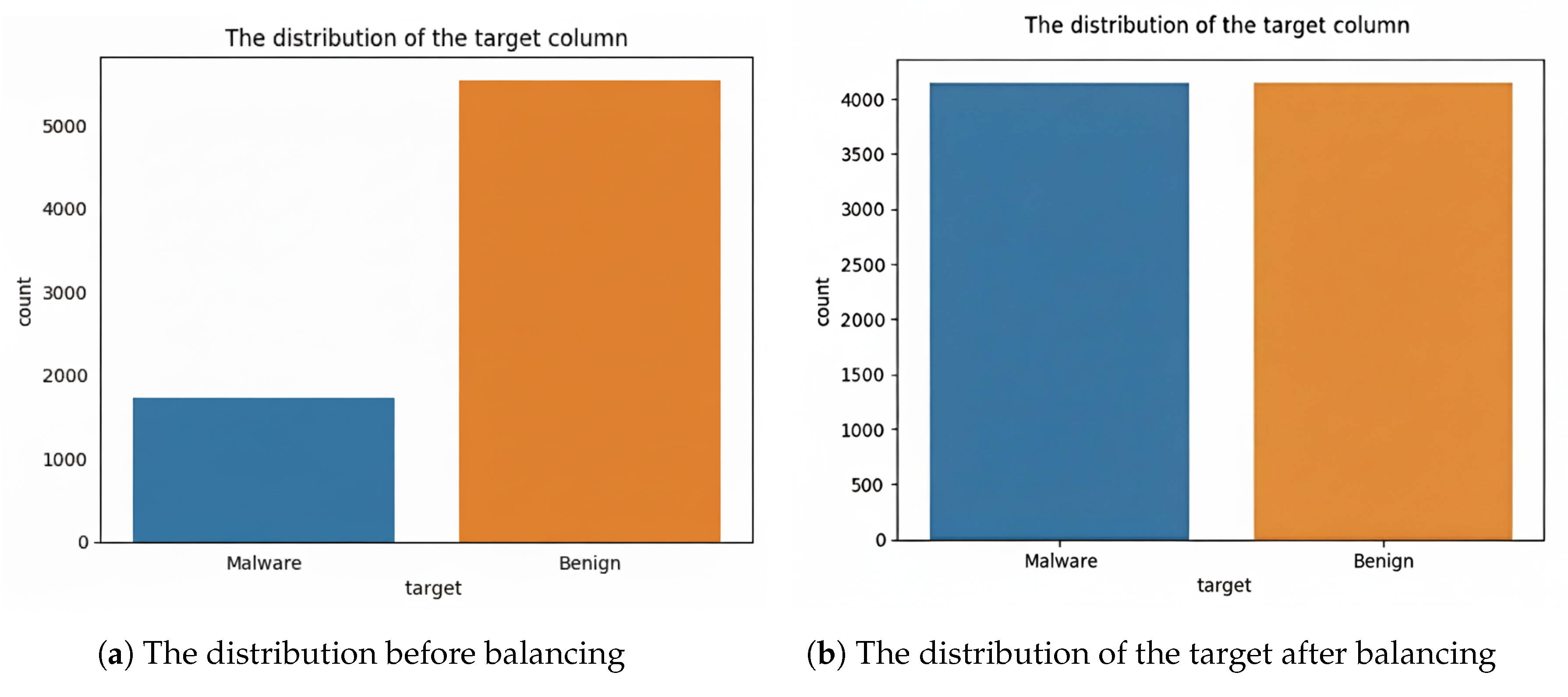
This dataset comprises 15,036 samples (7260 post-duplicate removal) across 216 features (int64/object types), labeled as malware (S) or benign (B). It covers diverse malware via permissions, API calls, intents, and URLs. Initial class imbalance (benign-dominant) was addressed via random oversampling to equalize classes, preventing majority-class bias (Figure 2 shows pre-balancing; and post-balancing).

4.2.2. CIC-InvesAndMal2019 Dataset [44]

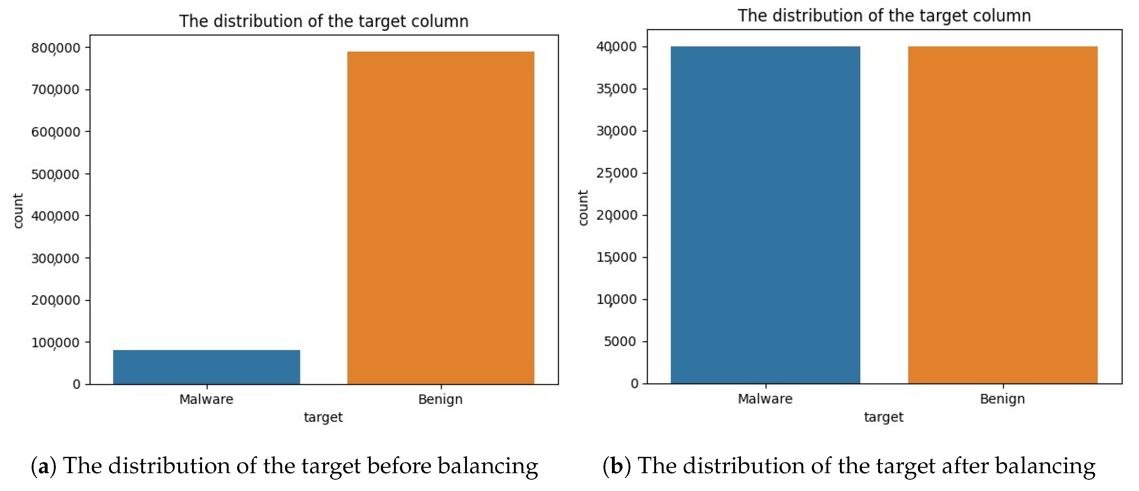
The dataset, sourced from multiple CSV files, contains approximately 800,000 benign samples and 80,000 malware samples across various families, with over 70 static and dynamic features. Columns with a single unique value were removed, and class imbalance was addressed by downsampling benign samples to 40,000, using a random seed of 42, and applying random oversampling to malware samples. This process resulted in balanced distributions, as illustrated in Figure 3, which compares the dataset before and after balancing. Such preprocessing ensures unbiased training [61].

4.3. Data Preprocessing and Model Architectures

Table 5 presents a comparative summary of the implemented deep learning architectures across two datasets (Android and CIC) and two experimental scenarios for each dataset. The table consolidates the structural details of five models: DNN, CNN, RNN, LSTM, and CNN-LSTM, highlighting their layers, the number of neurons, and training epochs.
For the Android dataset, both scenarios employed 100 epochs. Scenario 1 configurations focused on moderate depth, with CNN and CNN-LSTM using smaller convolutional kernels and fewer layers, while RNN and LSTM models relied on higher neuron counts (128–256). In contrast, Scenario 2 introduced deeper CNN layers with larger convolutional feature maps (128, 128), stronger dropout rates (0.5, 0.4), and more extensive use of batch normalization, reflecting a shift towards more regularized and complex architectures to enhance generalization.
For the CIC dataset, Scenario 1 architectures were relatively lightweight, with smaller neuron counts (32–64) and reduced convolutional complexity. This setup suggests that the initial focus was on computational efficiency and faster convergence. Scenario 2, however, scaled the architectures substantially, employing larger neuron counts (up to 256), deeper CNN layers with three convolutional stages, and stronger dropout regularization. The CNN-LSTM in this scenario also combined temporal modeling with higher-capacity convolutional feature extraction, reflecting the dataset’s complexity.
Overall, the architectural adjustments demonstrate a systematic attempt to balance computational efficiency (Scenario 1) with enhanced feature learning and generalization (Scenario 2), providing insights into how architectural depth and regularization strategies impact malware detection performance across heterogeneous datasets.
The progression from Scenario 1 to Scenario 2 in both datasets illustrates an experimental design that gradually increases model complexity, regularization, and representational power.

5. Results and Analysis

5.1. Computational Environment

The experimental environment was conducted using Google Colab with Python3.10 on the Google compute engine backend equipped with 12.7 GB RAM and 107.7 GB disk.
We first loaded the required analytical, visualization, and predictive modeling libraries such as Scikit-learn 1.6.0, Pandas 2.2.3, Seaborn 0.13.2, and numpy 1.26.4 to interact with Python’s logic and math libraries and handle several essential regressions and classifications [62], data manipulation and analysis, access datasets, visualization libraries like matplotlib [63], and support mathematics, statistics, and data manipulation. Also, we used Keras, which is an open-source API for high-level neural networks. Finally, we used the TensorFlow library, which provides powerful general-purpose numerical computation functions, including machine learning.

5.2. Performance Evaluation

Metrics included accuracy, F1-score, precision, recall, training/testing time, and CPU usage. Confusion matrices and learning curves (train/validation loss/accuracy) assessed convergence and bias.

5.2.1. Android Malware Dataset

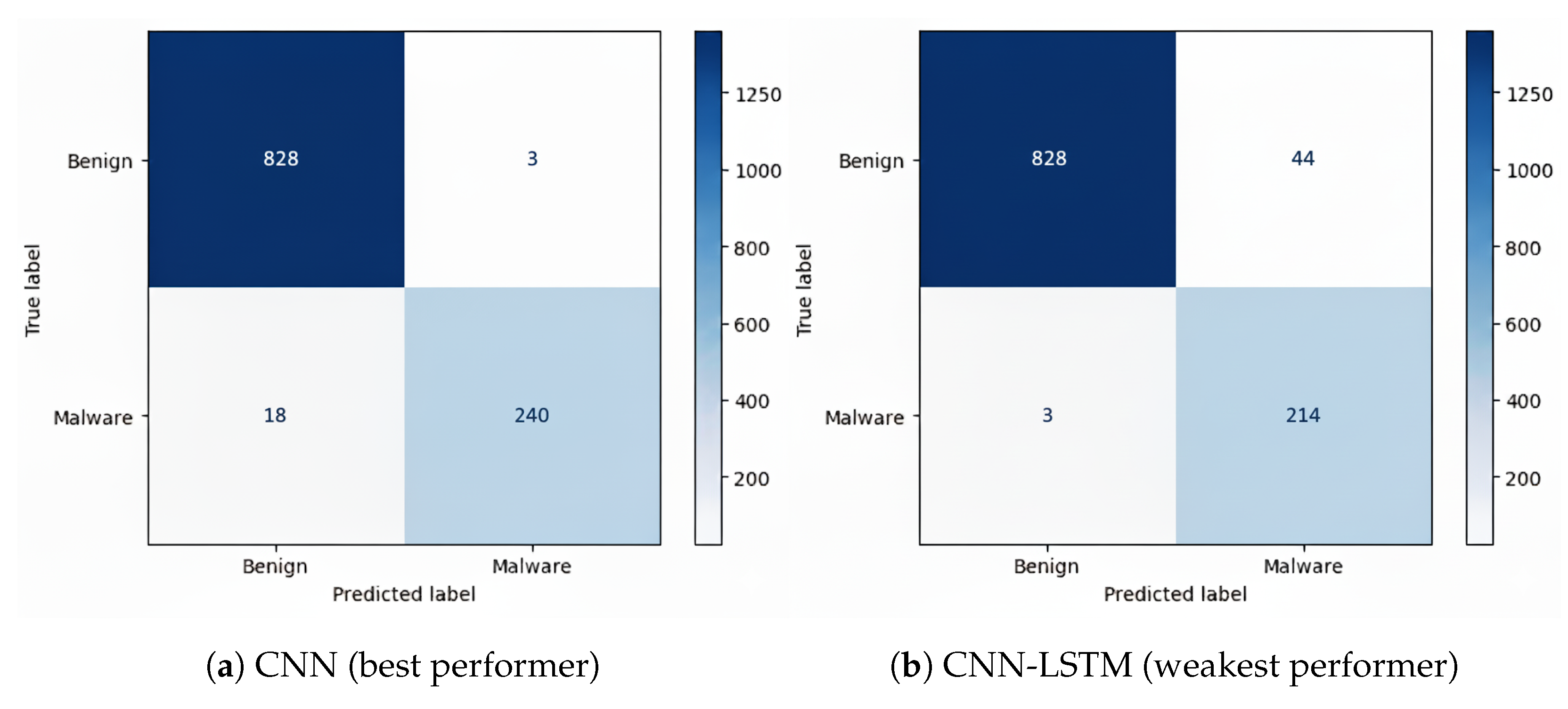
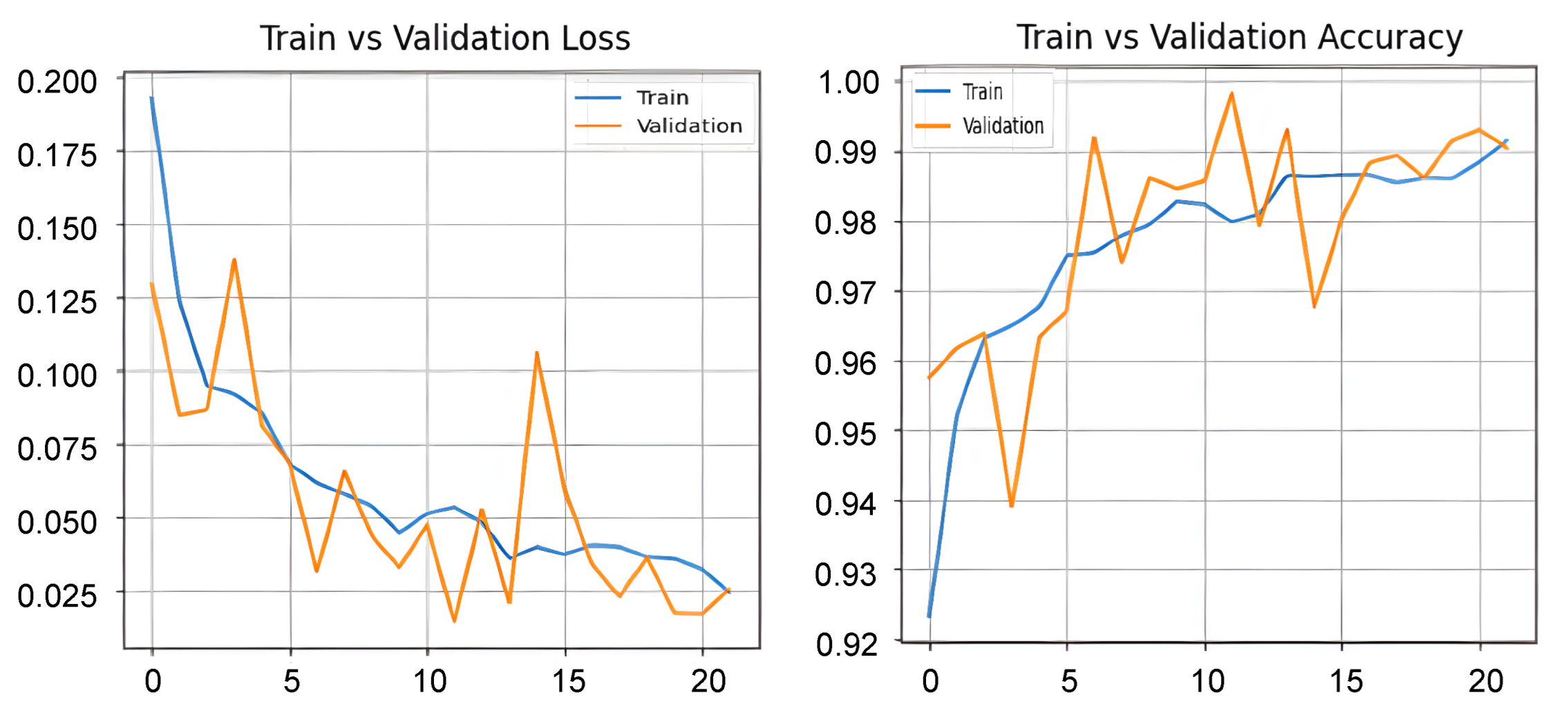
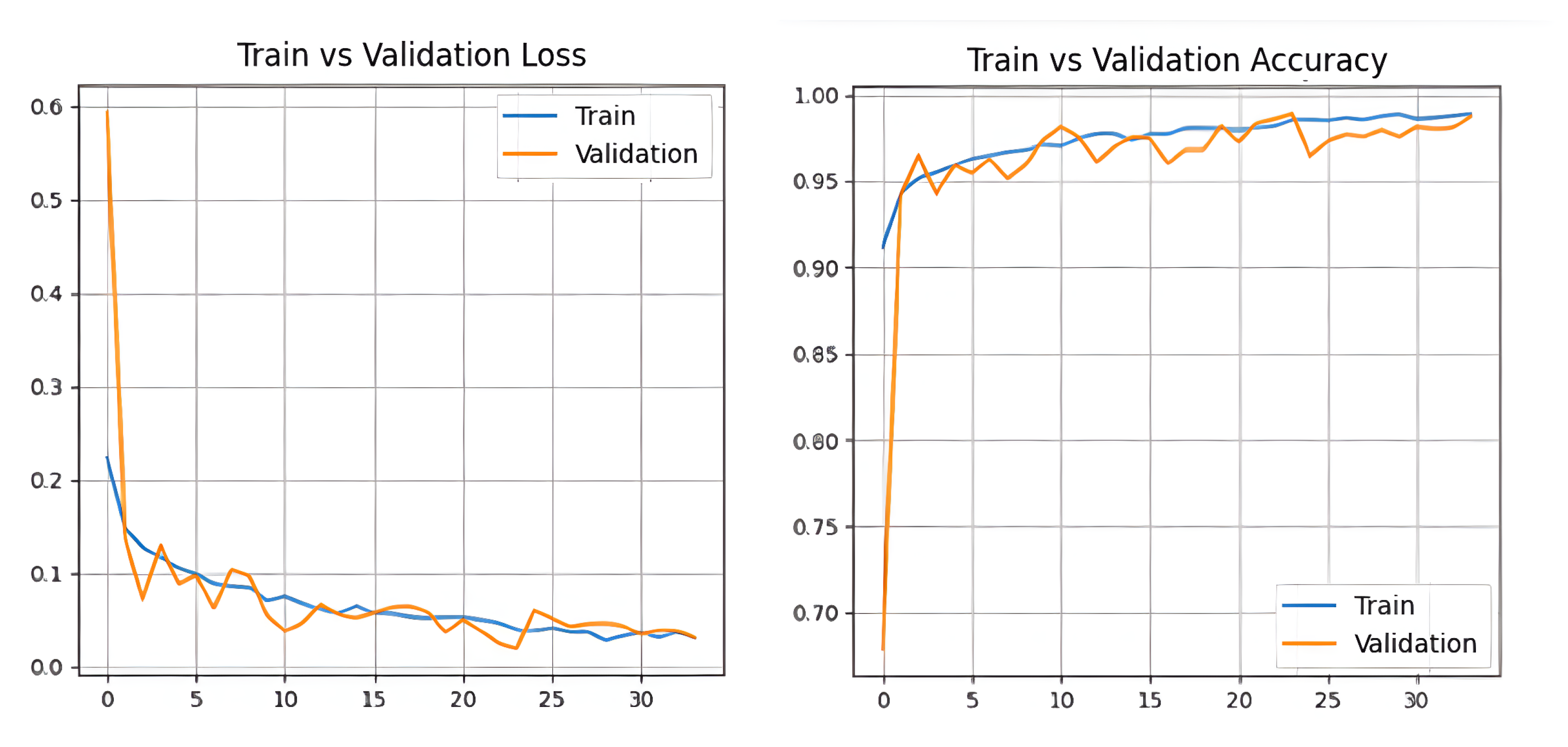
Scenario 1 (No Selection): All models achieved accuracies above 96%. The CNN and LSTM models attained the highest performance (98.07% accuracy, F1-score = 98%), with relatively few misclassifications (CNN: 3 false positives and 18 false negatives; LSTM: 7 false negatives). In contrast, the CNN-LSTM model exhibited the highest number of false positives (44), indicating reduced precision despite strong overall accuracy. The learning curves demonstrated consistent convergence across models, with CNN and LSTM showing minimal overfitting (Figure 4 and Figure 5). Also, CNN outperformed the other models in terms of computational efficiency, achieving the fastest execution time and the lowest CPU utilization (Table 6).
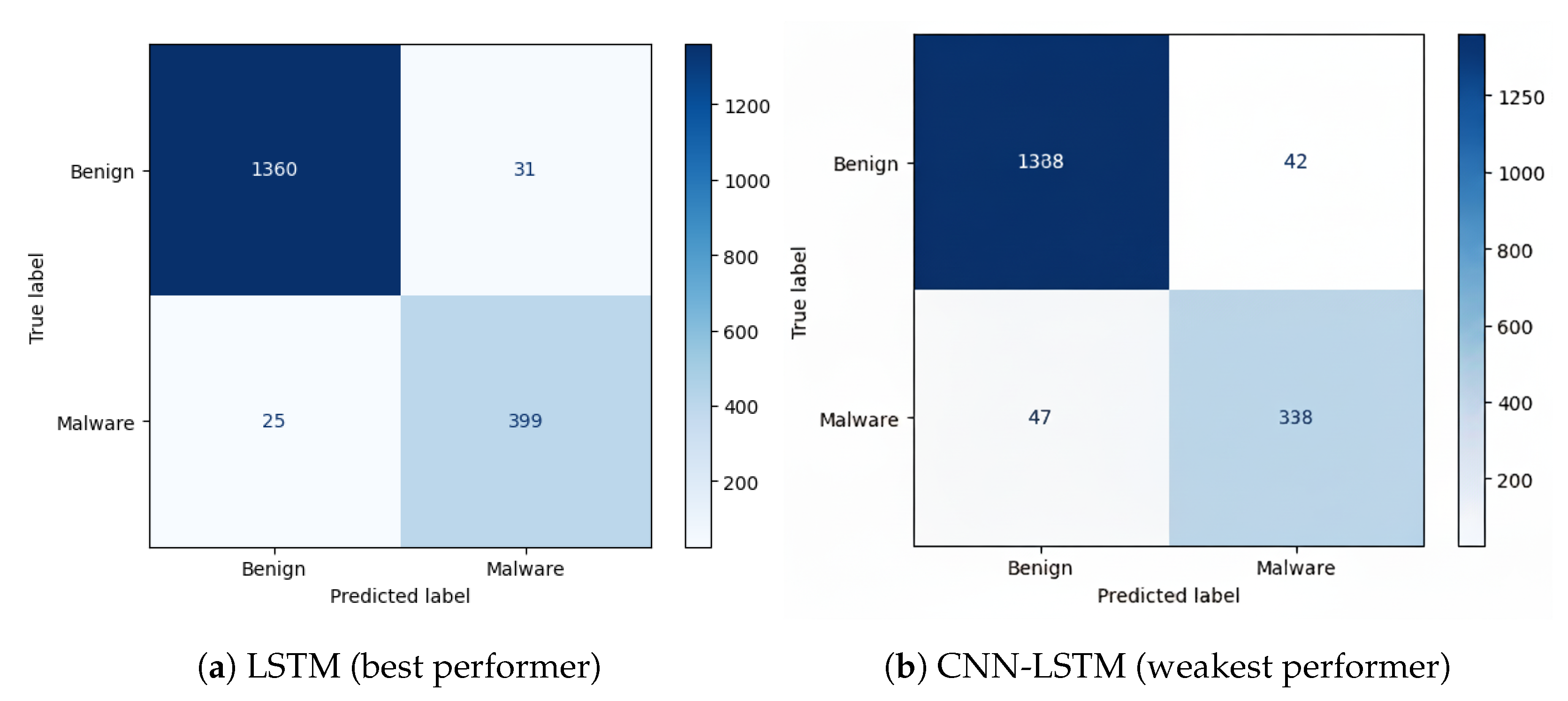
Scenario 2 (With Selection): The LSTM model achieved the highest performance (96.86% accuracy, F1-score = 97%), correctly identifying 399 true positives with 26 false negatives. However, overall accuracy decreased by approximately 1.4% compared to Scenario 1, likely due to the loss of discriminative features following feature selection. Among all models, the RNN demonstrated the most efficient computational profile, minimizing CPU utilization while maintaining competitive predictive performance (Table 7; Figure 6 and Figure 7).

5.2.2. CIC-InvesAndMal2019 Dataset

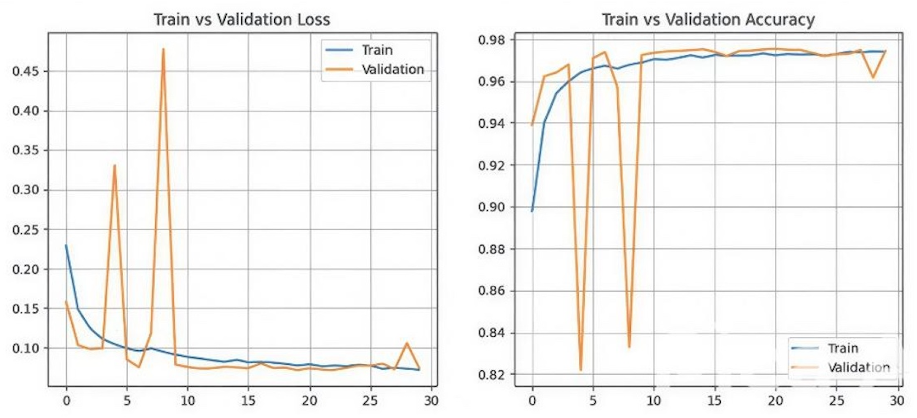
Scenario 1 (No Selection): Both CNN and CNN-LSTM achieved the highest performance (97.14–97.20% accuracy), with consistently low false positive and false negative rates. In contrast, the RNN model exhibited elevated false negatives, despite maintaining a strong recall rate. Overall, the learning curves demonstrated stable convergence across models, indicating robust training behavior (Table 8; Figure 8 and Figure 9).
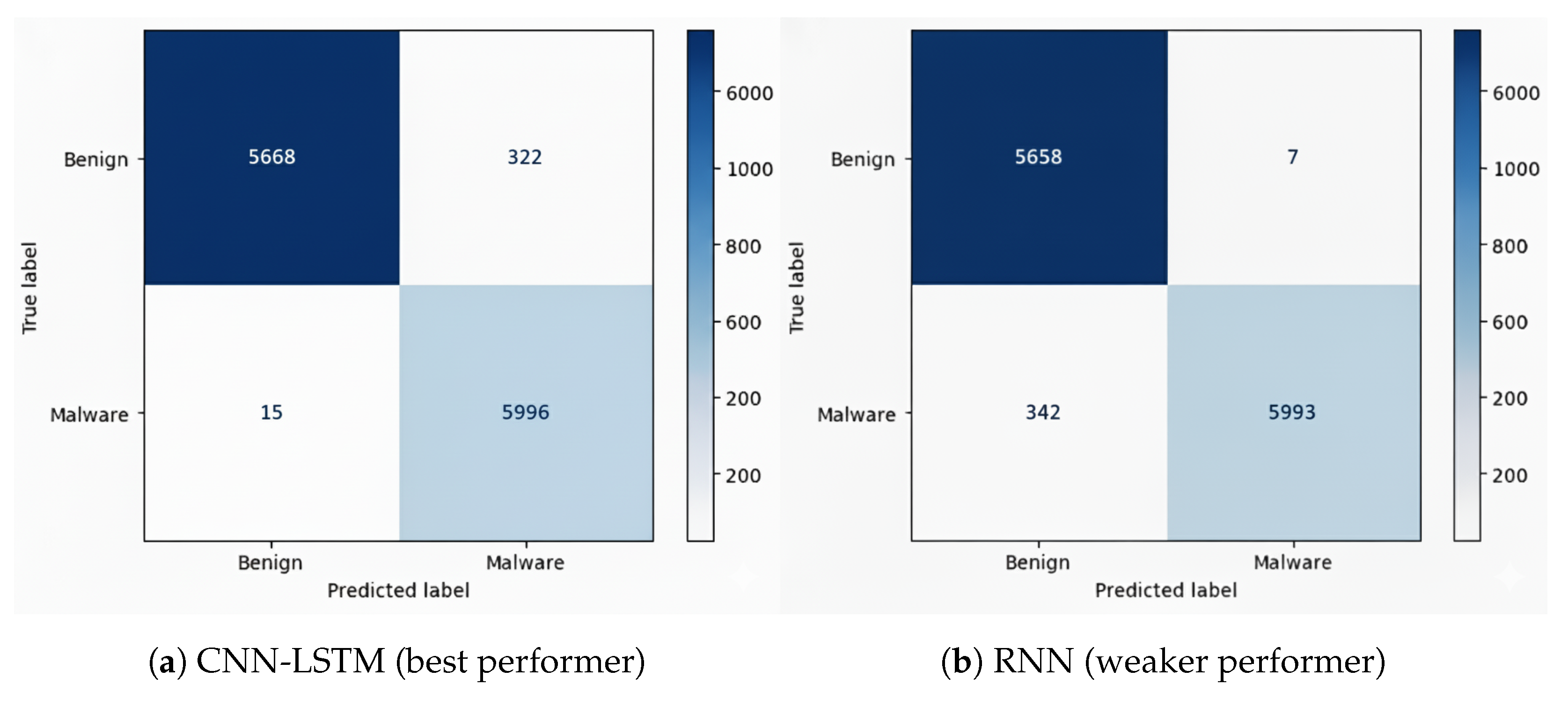
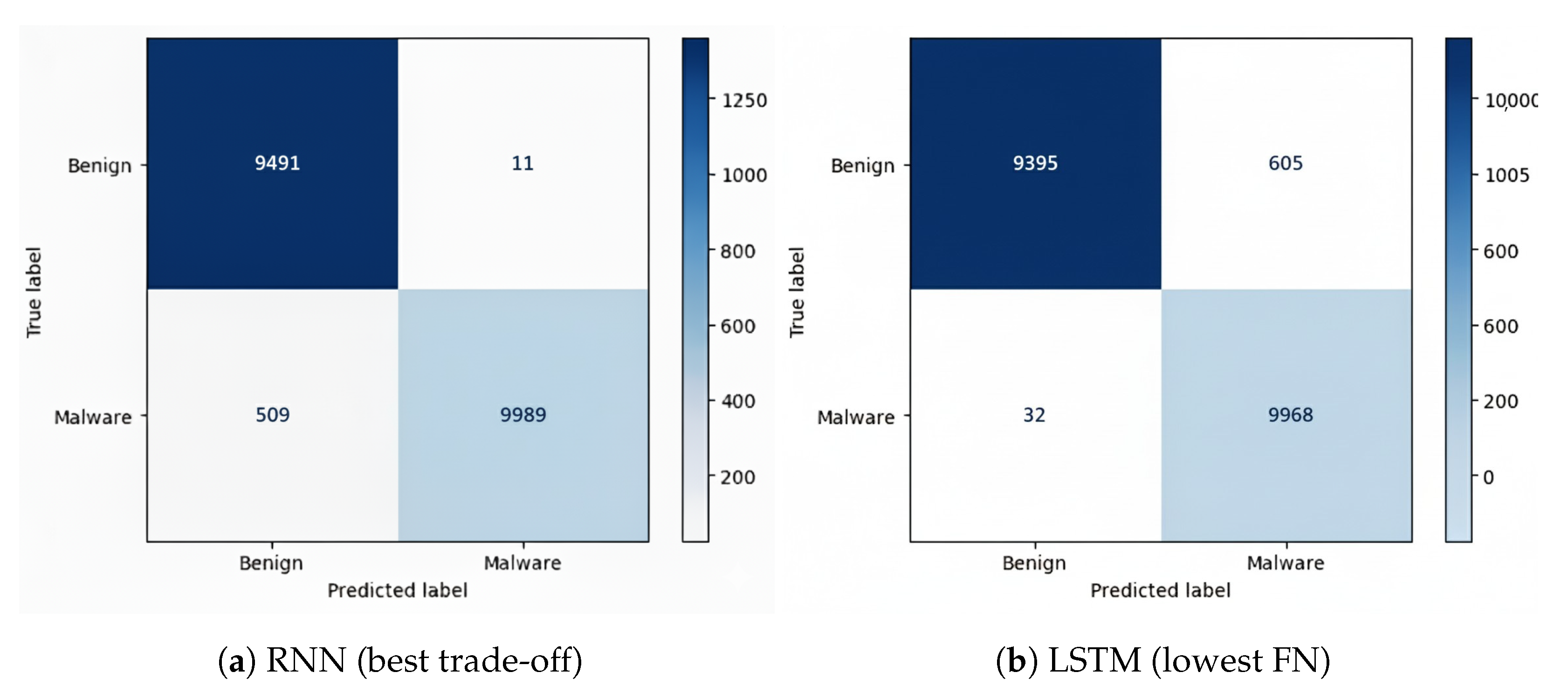
Scenario 2: With Feature Selection As shown in Figure 10, the confusion matrix analysis shows that all models achieved strong performance, but with varying trade-offs between false positives (FP) and false negatives (FN).
  • RNN achieved the best overall balance, with the lowest FP (11) and relatively low FN (509).
  • CNN also performed well, with the lowest FP (11) but higher FN (536).
  • LSTM minimized FN (32), but at the cost of higher FP (505).
  • DNN showed balanced but slightly weaker results compared to RNN and CNN.
  • CNN-LSTM had higher FP (481) than most models, though FN (36) was comparable to LSTM.
Overall, RNN provided the best trade-off, CNN favored low false alarms, while LSTM and CNN-LSTM prioritized minimizing missed malware.
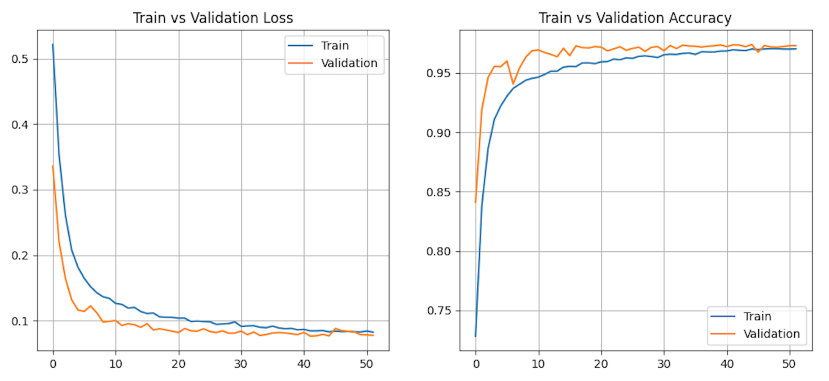
As mentioned in the first scenario, Figure 11 shows the learning curve for RNN, the model with the best overall trade-off. The curve indicates steady convergence, reflecting consistent training behavior.
The Table 9 shows that all models achieved high performance, with accuracies ranging from 96.82% (LSTM) to 97.42% (CNN-LSTM) and F1-scores closely aligned, indicating consistent detection capability. Precision values (94.28–95.39%) show low false positives, while recall values (99.64–99.89%) indicate most true malware instances were correctly identified. CNN and CNN-LSTM required the longest training times, whereas RNN and DNN were faster. LSTM had the fastest testing time (2.59 s), and CNN-LSTM offered a good balance of accuracy and efficiency. Overall, CNN-LSTM achieved the best overall performance, LSTM provided rapid inference, RNN was light on resources, and DNN served as a stable baseline.

5.3. Statistical Reliability and Aggregated Performance Analysis

Each experiment was repeated five times using different random seeds to ensure statistical reliability and reproducibility. For each model and dataset configuration, we report the mean and standard deviation across these runs. The resulting averages summarized in Table 10 confirm that the proposed framework delivers stable detection performance across multiple architectures and preprocessing scenarios.
Across all configurations, the models achieve an average accuracy of 96.91 % ± 0.82 , with an F1-score of 96.93 % ± 0.81 and a precision of 96.46 % ± 1.05 . Recall remains consistently high at 97.90 % ± 1.48 .
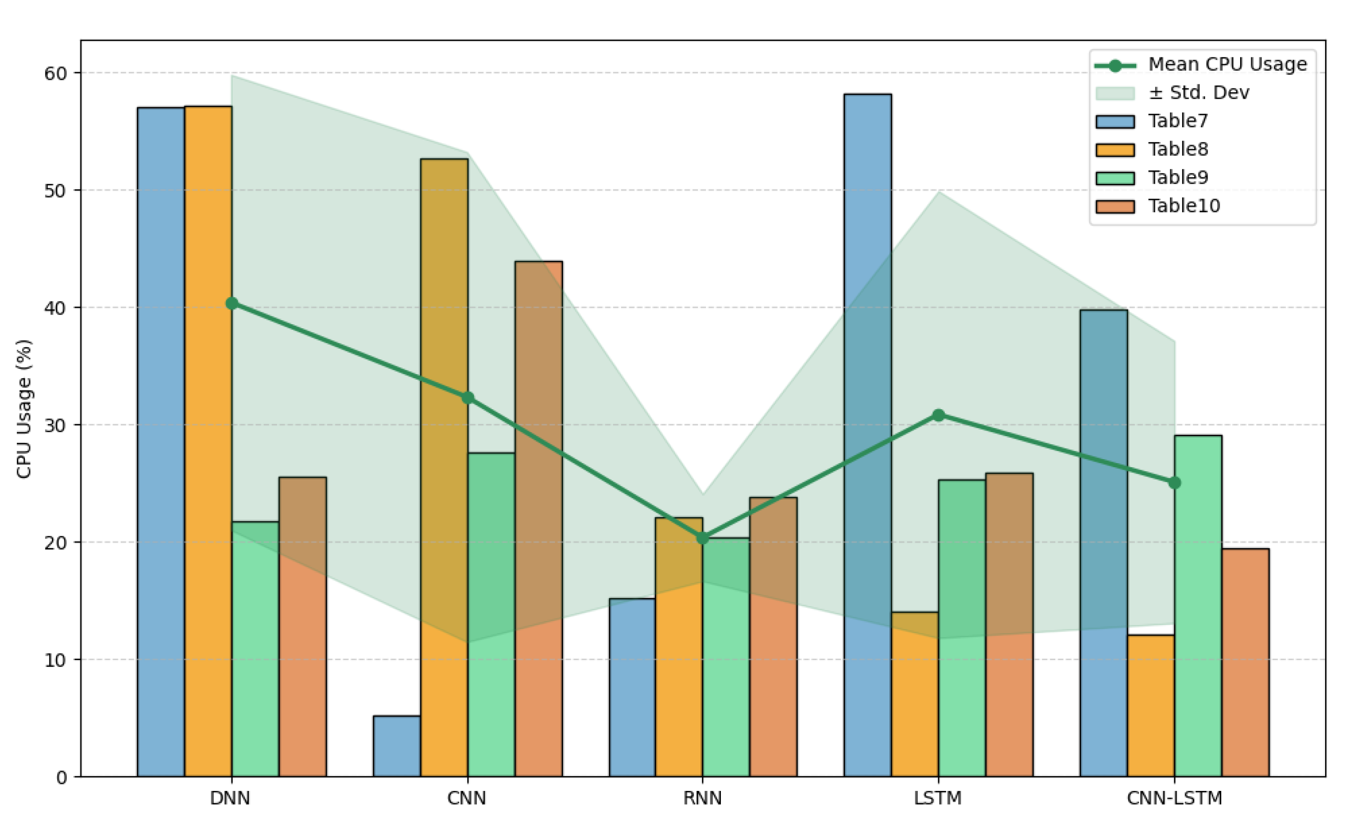
Figure 12 shows how CPU usage varies among the five models. CNN and hybrid CNN-LSTM architectures place heavier demands on processing power, while RNN and DNN consistently use less CPU. Overall, CPU utilization ranges from about 5% to 58%, depending on both the model design and the dataset type (Android or CIC). This balance between accuracy and efficiency ensures real-time or near-real-time feasibility for on-device inference.
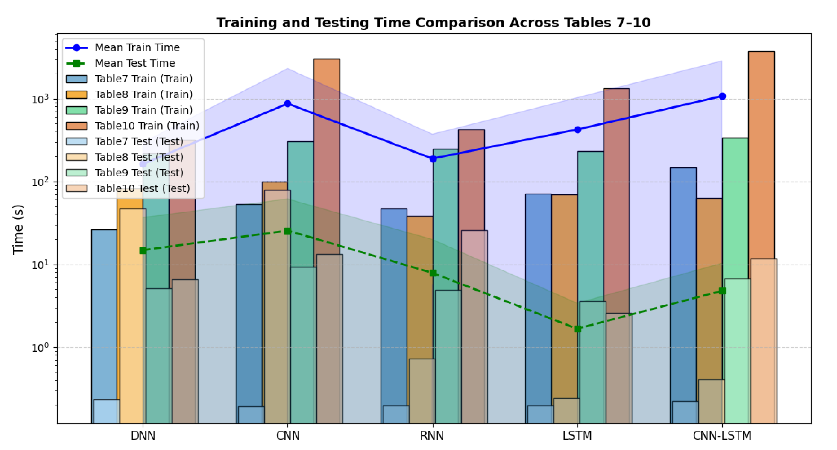
The comparison of training and testing times in Figure 13 shows clear differences in computational demand across the models. Training complexity shifts with model depth and dataset size, averaging 1112.18 s ± 1020.25, while testing stays lightweight at 25.31 s ± 12.05. This consistent inference efficiency confirms the suitability of the proposed models for resource-constrained deployments, maintaining a practical trade-off between accuracy and runtime cost.
These findings demonstrate consistent performance with limited variability across models and datasets, confirming the framework’s robustness, reproducibility, and efficiency under diverse computational conditions.

6. Android App Deployment

We integrated the proposed models into an Android app using TensorFlow Lite and tested them on a Pixel 8 emulator running Android 14.0. The emulator used an 8-core ARM Cortex-A78 processor and 4 GB RAM. We measured performance with the Android Studio Profiler. During on-device evaluation, we collected performance metrics, CPU utilization, and inference latency. The Supplementary Materials include the source code and mobile-testing scripts used in this study.

6.1. Model Conversion and Optimization

Trained Keras models were converted to TensorFlow Lite (.tflite) for on-device inference, using supported ops to minimize latency/privacy risks. The AI Malware Detection app (Android Studio 2025.2.1) serves as a sandbox for APK scanning, loading models dynamically based on CPU (e.g., lighter for high load). CNN was prioritized over LSTM for deployment: CNNs excel at spatial patterns (e.g., permission matrices as images), require fewer parameters/resources, and enable real-time scanning without sequential overhead.
The CPU usage (%) values represent total processor utilization aggregated over all device cores, as reported by the Android Studio Profiler. The values were normalized to the device’s maximum capacity (100 %), averaged over 30 inference runs to minimize transient fluctuations. The adaptive model-selection algorithm stayed active throughout deployment. But under normal CPU conditions, the system chose the CNN model by default because it offered the best balance between detection accuracy and inference speed. When CPU load passed the preset limits, the selector automatically switched to lighter models to keep the system responsive.

6.2. Deployment Results

Table 11 summarizes the app performance test results of five models (CNN, DNN, LSTM, CNN-LSTM, and RNN) on mid-range devices. Each model was evaluated using valid test images and compared in terms of accuracy, inference time, and reliability.
Also, the Table 11 reports the expected versus actual outputs, accuracy percentages, inference times, qualitative remarks, and final pass/fail outcomes. The CNN model achieved the highest accuracy with strong consistency, while other models demonstrated varying trade-offs between speed and accuracy. Mainly, the key results are:
  • CNN: Achieved the best overall performance with an accuracy of 98.5% and a reasonable inference time of 45 ms, making it the most reliable model.
  • DNN: Delivered faster inference (38 ms) but lower accuracy (91.3%), which was still acceptable, leading to a Pass outcome.
  • LSTM: Produced the lowest performance, with an accuracy of 87.6% and the slowest inference (105 ms), resulting in a Fail.
  • CNN-LSTM: Balanced accuracy (94.2%) and inference time (68 ms), representing a suitable trade-off between speed and reliability.
  • RNN: Showed unstable predictions with the lowest accuracy (83.9%) and high inference time (97 ms), leading to a Fail.
In summary, the CNN model is the most suitable choice for deployment on mid-range devices, followed by CNN-LSTM as a balanced alternative. LSTM and RNN are not recommended due to their poor accuracy and latency issues.

7. Discussion

The results demonstrate that deep learning models are effective for mobile malware detection, with CNN and LSTM standing out as the most promising candidates. Prior studies in mobile malware detection using machine learning have reported accuracies ranging from 85% to 95% [59]. More recent deep learning approaches have improved detection rates but often lack deployment evaluations [60]. In contrast, the proposed framework demonstrated superior performance across both datasets while incorporating additional system-level considerations as shown in Table 12 and Table 13.
For the Android dataset, our models matched or outperformed prior work. Specifically, the LSTM achieved 98.07% accuracy (without feature selection), closely aligning with the 98.3% reported by Alomari et al. [48], while outperforming their feature-selected setting (96.86% vs. 94.59%). Furthermore, our evaluation incorporated CPU utilization and testing time, metrics that were not addressed in their study. The application of oversampling to balance the dataset further enhanced the generalization capability compared to non-balanced approaches [38].
On the CIC dataset, our best-performing model (LSTM, without feature selection) achieved 97.09% accuracy, trailing the 98.80% reported by Calik et al. [64]. However, unlike their study, our framework explicitly accounted for mobile deployment constraints, including feature reduction and runtime performance, which contribute to practical applicability.
The difference comes from the characteristics of the datasets. CNN-LSTM performs poorly on the Android ML dataset that contains only static data with little temporal context, but it performs well on the CIC-InvesAndMal2019 dataset, which includes both static and dynamic behavioral features that let the model use its strength in sequential learning.
Finally, graph-based approaches such as those proposed by Guan et al. [65] provide valuable insights into malware family relationships but do not address the multi-model and hybrid architecture perspective considered in this work. These comparisons underscore the novelty and practical relevance of our framework in balancing accuracy with deployment feasibility.
A major strength of this framework is its adaptability. CNN is suitable for resource-constrained real-time use, while LSTM provides higher accuracy for offline or server-assisted scenarios.

8. Conclusions

The study primarily focused on designing and testing a robust architecture for identifying mobile malware using deep learning models, including DNN, CNN, RNN, LSTM, and CNN-LSTM. Their performance was evaluated with metrics such as accuracy, F1-score, precision, recall, training/testing time, and CPU usage. Two datasets were used to assess model performance and select the most accurate model for detecting mobile malware.
Our results show that CNN works best as the default choice for mid-range devices, balancing accuracy and latency under normal load. When the CPU has extra capacity, CNN-LSTM improves accuracy with only a small latency cost. Under heavy load, the selector shifts smoothly to lighter models like RNN or DNN to keep on-device responses fast. In this context, resilience refers to the framework’s ability to keep its detection features operational even when computational resources on mobile devices fluctuate.
Finally, the AI Malware Detection application demonstrates the integration of deep learning, image processing, and responsive interface design. It efficiently detects images, provides real-time or near-real-time (depending on the device’s interactive latency) feedback, and delivers consistent performance across devices.
The strength of this work is not just in its model accuracy. Rather, it lies in how it brings together management and benchmarking into a single dynamic process that chooses models based on device load, then proves its worth through deployment on Android devices using TensorFlow Lite. This complete evaluation links theory to real-world performance and offers a solid, repeatable base for developing future adaptive, energy-efficient malware detection systems.
In future research, we will aim to explore larger, continuously updated datasets to capture evolving malware and to test how well the models handle obfuscated and adversarial malware samples to strengthen their resistance to attacks. Also, we will study adversarial robustness and privacy-preserving detection techniques (e.g., federated learning) to further strengthen the resilience of the detection model. Finally, further research is needed to analyze the forensic admissibility of the model in identifying attack timing and to extend the deployment to diverse devices and IoT endpoints in several application domains [66].

Supplementary Materials

The following supporting information can be downloaded at: https://github.com/Aysha-Alfaw/AI-Malware-detection-for-mobile-device (accessed on 10 November 2025).

Author Contributions

Conceptualization, A.A. (Aysha Alfaw), A.A. (Aymen Akremi) and M.R.; methodology, A.A. (Aysha Alfaw), A.A. (Aymen Akremi), and M.R.; software, A.A. (Aysha Alfaw); validation, A.A. (Aysha Alfaw), A.A. (Aymen Akremi), and M.R.; formal analysis, A.A. (Aysha Alfaw), A.A. (Aymen Akremi), and M.R.; investigation, A.A. (Aysha Alfaw), A.A. (Aymen Akremi), and M.R.; resources, A.A. (Aysha Alfaw) and A.A. (Aymen Akremi); data curation, A.A. (Aysha Alfaw) and A.A. (Aymen Akremi); writing—original draft preparation, A.A. (Aysha Alfaw), A.A. (Aymen Akremi), and M.R.; writing—review and editing, A.A. (Aymen Akremi) and M.R.; visualization, A.A. (Aysha Alfaw) and A.A. (Aymen Akremi); supervision, A.A. (Aymen Akremi) and M.R.; project administration, A.A. (Aymen Akremi) and M.R.; funding acquisition, A.A. (Aymen Akremi). All authors have read and agreed to the published version of the manuscript.

Funding

This research work was funded by Umm Al-Qura University, Saudi Arabia under grant number: 25UQU4361220GSSR03.

Institutional Review Board Statement

Not applicable.

Informed Consent Statement

Not applicable.

Data Availability Statement

Data available in a publicly accessible repository. URL of the first dataset (Android Malware Dataset for Machine Learning) is at https://www.kaggle.com/datasets/shashwatwork/android-malware-dataset-for-machine-learning (accessed on 18 November 2025). The URL of the second dataset (CIC-InvesAndMal2019 Dataset) is at https://www.kaggle.com/datasets/malikbaqi12/cic-invesandmal2019-dataset (accessed on 18 November 2025).

Acknowledgments

The authors extend their appreciation to Umm Al-Qura University, Saudi Arabia, for funding this research work through grant number: 25UQU4361220GSSR03.

Conflicts of Interest

The authors declare no conflicts of interest.

Abbreviations

The following abbreviations are used in this manuscript:
Indicators of CompromiseIoC
Deep Neural NetworkDNN
Convolutional Neural NetworkCNN
Long Short-Term MemoryLSTM
Applicationapp
CICAndMal2019CIC

References

  1. Khanachivskyi, O. How Many Apps Are in the Google Play Store in 2025? A Look at the Mobile Landscape. 2025. Available online: https://litslink.com/blog/how-many-apps-are-in-the-google-play-store (accessed on 10 September 2025).
  2. Anees, A.; Hussain, I.; Khokhar, U.M.; Ahmed, F.; Shaukat, S. Machine learning and applied cryptography. Secur. Commun. Netw. 2022, 2022, 1–3. [Google Scholar] [CrossRef]
  3. Mbunge, E.; Muchemwa, B.; Batani, J.; Mbuyisa, N. A review of deep learning models to detect malware in Android applications. Cyber Secur. Appl. 2023, 1, 100014. [Google Scholar] [CrossRef]
  4. Preuveneers, D.; Joosen, W. Sharing machine learning models as indicators of compromise for cyber threat intelligence. J. Cybersecur. Priv. 2021, 1, 140–163. [Google Scholar] [CrossRef]
  5. Su, X.; Xiao, L.; Li, W.; Liu, X.; Li, K.C.; Liang, W. DroidPortrait: Android malware portrait construction based on multidimensional behavior analysis. Appl. Sci. 2020, 10, 3978. [Google Scholar] [CrossRef]
  6. Yerima, S.Y. High Accuracy Detection of Mobile Malware Using Machine Learning. Electronics 2023, 12, 1408. [Google Scholar] [CrossRef]
  7. Chowdhury, M.N.U.R.; Haque, A.; Soliman, H.; Hossen, M.S.; Fatima, T.; Ahmed, I. Android malware Detection using Machine learning: A Review. arXiv 2023, arXiv:2307.02412. [Google Scholar] [CrossRef]
  8. Augello, A.; De Paola, A.; Re, G.L. M2FD: Mobile malware federated detection under concept drift. Comput. Secur. 2025, 152, 104361. [Google Scholar] [CrossRef]
  9. Nayak, P.; Sharma, A. A review on machine learning in cryptography: Future perspective and application. In AIP Conference Proceedings; AIP Publishing LLC: Melville, NY, USA, 2025; Volume 3224, p. 020031. [Google Scholar]
  10. Catakoglu, O.; Balduzzi, M.; Balzarotti, D. Automatic extraction of indicators of compromise for web applications. In Proceedings of the 25th International Conference on World Wide Web, Montreal, QC, Canada, 11–15 April 2016; pp. 333–343. [Google Scholar]
  11. Zhou, S.; Long, Z.; Tan, L.; Guo, H. Automatic identification of indicators of compromise using neural-based sequence labelling. arXiv 2018, arXiv:1810.10156. [Google Scholar] [CrossRef]
  12. Asiri, M.; Saxena, N.; Gjomemo, R.; Burnap, P. Understanding indicators of compromise against cyber-attacks in industrial control systems: A security perspective. ACM Trans.-Cyber-Phys. Syst. 2023, 7, 1–33. [Google Scholar] [CrossRef]
  13. Akremi, A. A forensic-driven data model for automatic vehicles events analysis. PeerJ Comput. Sci. 2022, 8, e841. [Google Scholar] [CrossRef]
  14. Rouached, M.; Akremi, A.; Macherki, M.; Kraiem, N. Policy-Based Smart Contracts Management for IoT Privacy Preservation. Future Internet 2024, 16, 452. [Google Scholar] [CrossRef]
  15. Liu, Y.; Tantithamthavorn, C.; Li, L.; Liu, Y. Deep learning for android malware defenses: A systematic literature review. ACM Comput. Surv. 2022, 55, 1–36. [Google Scholar] [CrossRef]
  16. Song, Y.; Zhang, D.; Wang, J.; Wang, Y.; Wang, Y.; Ding, P. Application of deep learning in malware detection: A review. J. Big Data 2025, 12, 99. [Google Scholar] [CrossRef]
  17. Garg, S.; Baliyan, N. Comparative analysis of Android and iOS from security viewpoint. Comput. Sci. Rev. 2021, 40, 100372. [Google Scholar] [CrossRef]
  18. Senanayake, J.; Kalutarage, H.; Al-Kadri, M.O. Android mobile malware detection using machine learning: A systematic review. Electronics 2021, 10, 1606. [Google Scholar] [CrossRef]
  19. Akremi, A.; Sallay, H.; Rouached, M. An efficient intrusion alerts miner for forensics readiness in high speed networks. Int. J. Inf. Secur. Priv. (IJISP) 2014, 8, 62–78. [Google Scholar] [CrossRef]
  20. Aslan, Ö.A.; Samet, R. A comprehensive review on malware detection approaches. IEEE Access 2020, 8, 6249–6271. [Google Scholar] [CrossRef]
  21. Panman de Wit, J.; Bucur, D.; van der Ham, J. Dynamic detection of mobile malware using smartphone data and machine learning. Digit. Threat. Res. Pract. (DTRAP) 2022, 3, 1–24. [Google Scholar] [CrossRef]
  22. Senanayake, J.; Kalutarage, H.; Al-Kadri, M.O.; Petrovski, A.; Piras, L. Android source code vulnerability detection: A systematic literature review. ACM Comput. Surv. 2023, 55, 1–37. [Google Scholar] [CrossRef]
  23. Alromaihi, N.; Rouached, M.; Akremi, A. Design and Analysis of an Effective Architecture for Machine Learning Based Intrusion Detection Systems. Network 2025, 5, 13. [Google Scholar] [CrossRef]
  24. Ucci, D.; Aniello, L.; Baldoni, R. Survey of machine learning techniques for malware analysis. Comput. Secur. 2019, 81, 123–147. [Google Scholar] [CrossRef]
  25. Kaur, A.; Jain, S.; Goel, S.; Dhiman, G. A review on machine-learning based code smell detection techniques in object-oriented software system (s). Recent Adv. Electr. Electron. Eng. (Former. Recent Patents Electr. Electron. Eng. 2021, 14, 290–303. [Google Scholar] [CrossRef]
  26. Buczak, A.L.; Guven, E. A survey of data mining and machine learning methods for cyber security intrusion detection. IEEE Commun. Surv. Tutorials 2015, 18, 1153–1176. [Google Scholar] [CrossRef]
  27. Kolias, C.; Kambourakis, G.; Stavrou, A.; Voas, J. DDoS in the IoT: Mirai and other botnets. Computer 2017, 50, 80–84. [Google Scholar] [CrossRef]
  28. Meng, G.; Xue, Y.; Xu, Z.; Liu, Y.; Zhang, J.; Narayanan, A. Semantic modelling of android malware for effective malware comprehension, detection, and classification. In Proceedings of the 25th International Symposium on Software Testing and Analysis, Saarbrücken, Germany, 18–20 July 2016; pp. 306–317. [Google Scholar]
  29. Onwuzurike, L.; Mariconti, E.; Andriotis, P.; Cristofaro, E.D.; Ross, G.; Stringhini, G. Mamadroid: Detecting android malware by building markov chains of behavioral models (extended version). ACM Trans. Priv. Secur. (TOPS) 2019, 22, 1–34. [Google Scholar] [CrossRef]
  30. Mahindru, A.; Sangal, A. FSDroid:-A feature selection technique to detect malware from Android using Machine Learning Techniques: FSDroid. Multimed. Tools Appl. 2021, 80, 13271–13323. [Google Scholar] [CrossRef]
  31. Hasan, H.; Ladani, B.T.; Zamani, B. MEGDroid: A model-driven event generation framework for dynamic android malware analysis. Inf. Softw. Technol. 2021, 135, 106569. [Google Scholar] [CrossRef]
  32. Akremi, A. Software security static analysis false alerts handling approaches. Int. J. Adv. Comput. Sci. Appl 2021, 12, 1–10. [Google Scholar] [CrossRef]
  33. Liu, L.; Wang, B. Automatic malware detection using deep learning based on static analysis. In Proceedings of the Data Science: Third International Conference of Pioneering Computer Scientists, Engineers and Educators, ICPCSEE 2017, Changsha, China, 22–24 September 2017; Proceedings, Part I. pp. 500–507. [Google Scholar]
  34. Saxe, J.; Berlin, K. Deep neural network based malware detection using two dimensional binary program features. In Proceedings of the 2015 10th International Conference on Malicious and Unwanted Software (MALWARE), Fajardo, PR, USA, 20–22 October 2015; pp. 11–20. [Google Scholar]
  35. Xu, K.; Li, Y.; Deng, R.H.; Chen, K. DeepRefiner: Multi-layer Android Malware Detection System Applying Deep Neural Networks. In Proceedings of the 2018 IEEE European Symposium on Security and Privacy, London, UK, 24–26 April 2018; pp. 473–487. [Google Scholar] [CrossRef]
  36. Ullah, F.; Srivastava, G.; Ullah, S. A malware detection system using a hybrid approach of multi-heads attention-based control flow traces and image visualization. J. Cloud Comput. 2022, 11, 1–21. [Google Scholar] [CrossRef]
  37. Amin, M.; Tanveer, T.A.; Tehseen, M.; Khan, M.; Khan, F.A.; Anwar, S. Static malware detection and attribution in android byte-code through an end-to-end deep system. Future Gener. Comput. Syst. 2020, 102, 112–126. [Google Scholar] [CrossRef]
  38. Oak, R.; Du, M.; Yan, D.; Takawale, H.; Amit, I. Malware detection on highly imbalanced data through sequence modeling. In Proceedings of the 12th ACM Workshop on Artificial Intelligence and Security, London, UK, 15 November 2019; pp. 37–48. [Google Scholar]
  39. Alzaylaee, M.K.; Yerima, S.Y.; Sezer, S. DL-Droid: Deep learning based android malware detection using real devices. Comput. Secur. 2020, 89, 101663. [Google Scholar] [CrossRef]
  40. Mahindru, A.; Sangal, A. MLDroid—framework for Android malware detection using machine learning techniques. Neural Comput. Appl. 2021, 33, 5183–5240. [Google Scholar] [CrossRef]
  41. Vu, L.N.; Jung, S. AdMat: A CNN-on-matrix approach to Android malware detection and classification. IEEE Access 2021, 9, 39680–39694. [Google Scholar] [CrossRef]
  42. Arp, D.; Spreitzenbarth, M.; Hubner, M.; Gascon, H.; Rieck, K.; Siemens, C. Drebin: Effective and explainable detection of android malware in your pocket. In Proceedings of the NDSS, San Diego, CA, USA, 23–26 February 2014; Volume 14, pp. 23–26. [Google Scholar]
  43. Wei, F.; Li, Y.; Roy, S.; Ou, X.; Zhou, W. Deep ground truth analysis of current android malware. In Proceedings of the Detection of Intrusions and Malware, and Vulnerability Assessment: 14th International Conference, DIMVA 2017, Bonn, Germany, 6–7 July 2017; Proceedings 14. pp. 252–276. [Google Scholar]
  44. Lashkari, A.H.; Kadir, A.F.A.; Taheri, L.; Ghorbani, A.A. Toward Developing a Systematic Approach to Generate Benchmark Android Malware Datasets and Classification. In Proceedings of the 2018 International Carnahan Conference on Security Technology (ICCST), Montreal, QC, Canada, 22–25 October 2018; pp. 1–7. [Google Scholar] [CrossRef]
  45. Chen, K.; Wang, P.; Lee, Y.; Wang, X.; Zhang, N.; Huang, H.; Zou, W.; Liu, P. Finding unknown malice in 10 seconds: Mass vetting for new threats at the google-play scale. In Proceedings of the 24th {USENIX} Security Symposium ({USENIX} Security 15), Washington, DC, USA, 12–14 August 2015; pp. 659–674. [Google Scholar]
  46. Allix, K.; Bissyandé, T.F.; Klein, J.; Le Traon, Y. Androzoo: Collecting millions of android apps for the research community. In Proceedings of the 13th International Conference on Mining Software Repositories, Austin, TX, USA, 14–15 May 2016; pp. 468–471. [Google Scholar]
  47. Yerima, S.Y.; Sezer, S. DroidFusion: A Novel Multilevel Classifier Fusion Approach for Android Malware Detection. IEEE Trans. Cybern. 2019, 49, 453–466. [Google Scholar] [CrossRef]
  48. Alomari, E.S.; Nuiaa, R.R.; Alyasseri, Z.A.A.; Mohammed, H.J.; Sani, N.S.; Esa, M.I.; Musawi, B.A. Malware detection using deep learning and correlation-based feature selection. Symmetry 2023, 15, 123. [Google Scholar] [CrossRef]
  49. Alexandropoulos, S.A.N.; Kotsiantis, S.B.; Vrahatis, M.N. Data preprocessing in predictive data mining. Knowl. Eng. Rev. 2019, 34, e1. [Google Scholar] [CrossRef]
  50. Dogan, A.; Birant, D. Machine learning and data mining in manufacturing. Expert Syst. Appl. 2021, 166, 114060. [Google Scholar] [CrossRef]
  51. Acikmese, Y.; Alptekin, S.E. Prediction of stress levels with LSTM and passive mobile sensors. Procedia Comput. Sci. 2019, 159, 658–667. [Google Scholar] [CrossRef]
  52. Almahmoud, M.; Alzu’bi, D.; Yaseen, Q. ReDroidDet: Android malware detection based on recurrent neural network. Procedia Comput. Sci. 2021, 184, 841–846. [Google Scholar] [CrossRef]
  53. Bulut, I.; Yavuz, A.G. Mobile malware detection using deep neural network. In Proceedings of the 2017 25th Signal Processing and Communications Applications Conference (SIU), Antalya, Turkey, 15–18 May 2017; pp. 1–4. [Google Scholar]
  54. Kriegeskorte, N.; Golan, T. Neural network models and deep learning. Curr. Biol. 2019, 29, R231–R236. [Google Scholar] [CrossRef]
  55. Yeboah, P.N.; Baz Musah, H.B. NLP technique for malware detection using 1D CNN fusion model. Secur. Commun. Netw. 2022, 2022, 2957203. [Google Scholar] [CrossRef]
  56. Parameswaran Lakshmi, S. A lightweight 1-D CNN Model to Detect Android Malware on the Mobile Phone. Ph.D. Thesis, National College of Ireland, Dublin, Ireland, 2020. [Google Scholar]
  57. Sherstinsky, A. Fundamentals of recurrent neural network (RNN) and long short-term memory (LSTM) network. Phys. D Nonlinear Phenom. 2020, 404, 132306. [Google Scholar] [CrossRef]
  58. Lindemann, B.; Maschler, B.; Sahlab, N.; Weyrich, M. A survey on anomaly detection for technical systems using LSTM networks. Comput. Ind. 2021, 131, 103498. [Google Scholar] [CrossRef]
  59. Feizollah, A.; Anuar, N.B.; Salleh, R.; Wahab, A.W.A. A review on feature selection in mobile malware detection. Digit. Investig. 2015, 13, 22–37. [Google Scholar] [CrossRef]
  60. Wu, Y.; Li, M.; Zeng, Q.; Yang, T.; Wang, J.; Fang, Z.; Cheng, L. DroidRL: Feature selection for android malware detection with reinforcement learning. Comput. Secur. 2023, 128, 103126. [Google Scholar] [CrossRef]
  61. Mimura, M. Impact of benign sample size on binary classification accuracy. Expert Syst. Appl. 2023, 211, 118630. [Google Scholar] [CrossRef]
  62. Bisong, E.; Bisong, E. Introduction to Scikit-learn. Building Machine Learning and Deep Learning Models on Google Cloud Platform: A Comprehensive Guide for Beginners; Apress: Berkeley, CA, USA, 2019; pp. 215–229. [Google Scholar]
  63. McKinney, W. pandas: A foundational Python library for data analysis and statistics. Python High Perform. Sci. Comput. 2011, 14, 1–9. [Google Scholar]
  64. Calik Bayazit, E.; Koray Sahingoz, O.; Dogan, B. Deep learning based malware detection for android systems: A Comparative Analysis. Teh. Vjesn. 2023, 30, 787–796. [Google Scholar]
  65. Guan, J.; Jiang, X.; Mao, B. A method for class-imbalance learning in android malware detection. Electronics 2021, 10, 3124. [Google Scholar] [CrossRef]
  66. Akremi, A. ForensicTwin: Incorporating Digital Forensics Requirements Within a Digital Twin. Computers 2025, 14, 115. [Google Scholar] [CrossRef]
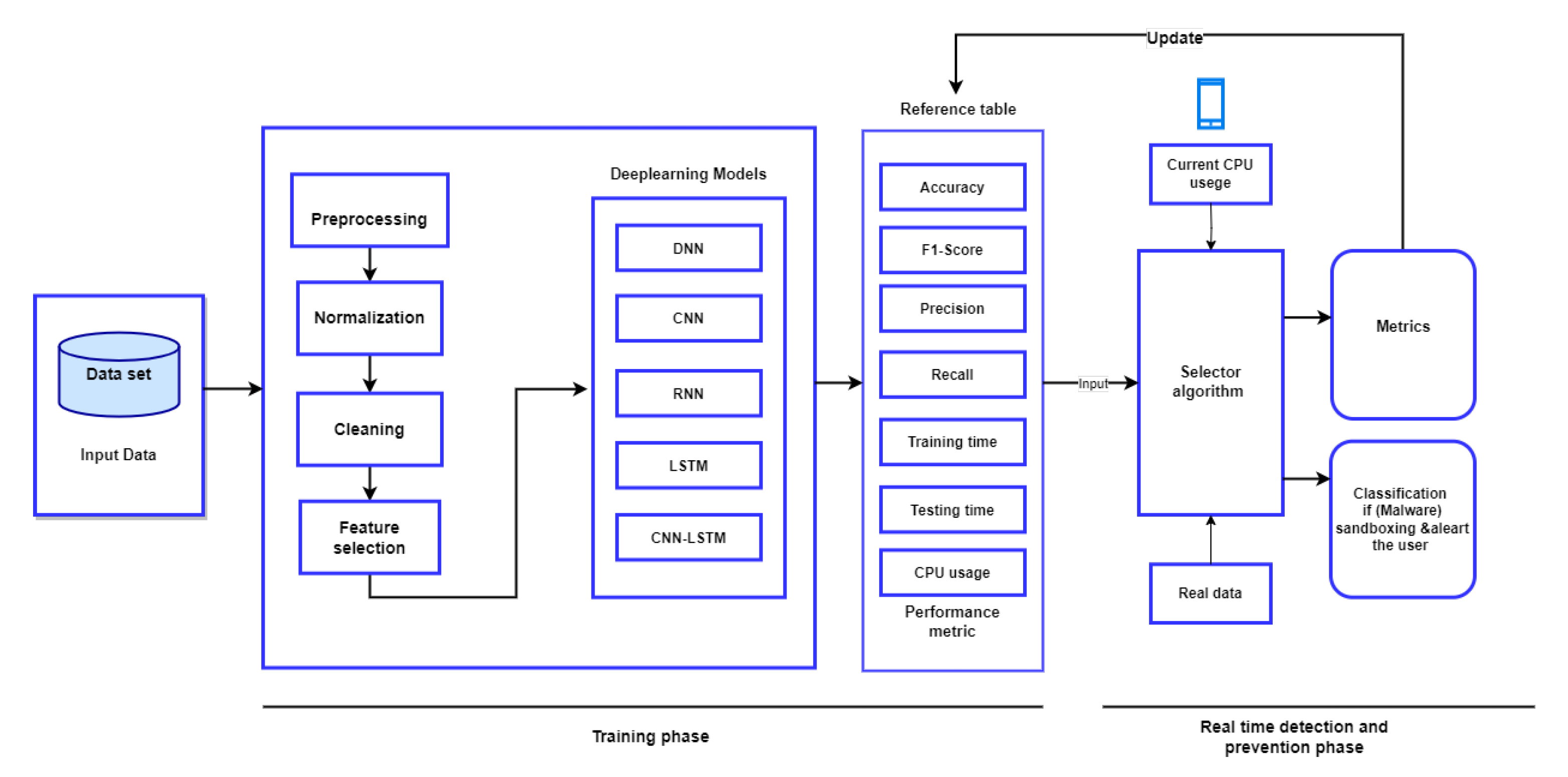
Figure 1. Proposed mobile malware detection architecture.
Futureinternet 17 00532 g001
Figure 2. Class distribution before and after balancing(first dataset).
Futureinternet 17 00532 g002
Figure 3. Class distribution before and after balancing (second dataset).
Futureinternet 17 00532 g003
Figure 4. Representative confusion matrices for Scenario 1 (Android dataset).
Futureinternet 17 00532 g004
Figure 5. Representative learning curve (CNN) for Scenario 1.
Futureinternet 17 00532 g005
Figure 6. Representative confusion matrices for Scenario 2 (Android dataset).
Futureinternet 17 00532 g006
Figure 7. Representative learning curve (LSTM) for Scenario 2.
Futureinternet 17 00532 g007
Figure 8. Representative confusion matrices for Scenario 1 (second dataset).
Futureinternet 17 00532 g008
Figure 9. Representative learning curve (CNN-LSTM) for Scenario 1.
Futureinternet 17 00532 g009
Figure 10. Representative confusion matrices for Scenario 2 (second dataset).
Futureinternet 17 00532 g010
Figure 11. Representative learning curve (RNN) for Scenario 2.
Futureinternet 17 00532 g011
Figure 12. CPU usage comparison across deep learning models on both Android and CIC datasets.
Futureinternet 17 00532 g012
Figure 13. Training and testing time comparison across deep learning models.
Futureinternet 17 00532 g013
Table 1. Machine learning-based malware detection approaches.
AuthorDetection ApproachFeature Extraction MethodDatasetML AlgorithmAccuracy
[28]Machine deterministic symbolism and semantic modeling for Android malware detection.Opcode/bytecode analysisDrebinRF97%
[29]Application call graphs modeled as Markov chains, extracting API call sequences with MaMaDroid.API call analysisDrebin, OldBenignRF94%
[30]Feature selection applied to static features for malware detection.Requested permissions, API calls, intents, URLs, strings200,000 Android appsLSSVM98.7%
[31]Decompilation, model discovery, transformation, integration, and event generation.Java class and intent analysisAMDMEGDroid91.6%
Table 2. Deep learning-based malware detection approaches.
AuthorDetection ApproachFeature Extraction MethodDatasetSelected DL ModelsAccuracy
[35]Applying two different detection layers to achieve efficient detection and validating with DeepRefiner.Opcode/bytecode analysisGoogle Play, VirusShare, MassVetLSTM97.74%
[36]Combining ACGs with malware images as a new feature extraction method.Bytecode analysisCIC-Inves, AndMal2019CNN99.27%
[37]Malware attributes detected by vectorizing opcodes with one-hot encoding before applying DL.Opcode analysisAMD, VirusShareBiLSTM99.9%
[38]Created a simulated real-world dataset (imbalanced) to evaluate malware detection with BERT.Opcode analysisGoogle PlayLSTM91.9%
[39]Used DynaLog to extract features from logs and DL Droid for classification.Code instrumentation analysis (Java)Intel SecurityDL99.6%
Table 3. Count of deep learning-based malware detection approaches.
AuthorDetection ApproachFeature Extraction MethodDatasetSelected DL ModelsAccuracy
[40]Feature selection for malware detection using ML/DL models.Java classes, API calls at runtime, permissionsAndroid Permissions Dataset, Security and Computer DatasetDL (MLDroid framework)98.8%
[41]Characterizing apps as images, creating adjacency matrices, then applying CNN with the AdMat framework.API calls, opcodes, information flowDrebin, AMDCNN98.2%
Table 4. Dataset sources for mobile malware.
DatasetTime of CollectionMalware SamplesSource
DREBINAugugst 2010–October 20125560https://drebin.mlsec.org/(accessed on 20 October 2025)
Android Malware Genome ProjectAugust 2010–October 20111260http://www.malgenomeproject.org(accessed on 10 March 2025)
ContagioDecember 2011–March 20131150https://contagiodump.blogspot.com
VirusShare2018–20204038https://virusshare.com(accessed on 10 March 2025)
CICAndMal20172017365https://www.unb.ca/cic/datasets/andmal2017.html (accessed on 12 March 2025)
MassVet2015127,429https://massvis.mit.edu (accessed on 12 March 2025)
VirusSign2011146https://www.virussign.com (accessed on 12 March 2025)
VirusTotal2012–2018Not availablehttps://www.virustotal.com (accessed on 10 March 2025)
AndroZooNot available1,000,000https://androzoo.uni.lu (accessed on 14 March 2025)
Android Malware Dataset for ML201815,036https://www.kaggle.com (accessed on 14 March 2025)
Table 5. Comparative Architectures across Scenarios and Datasets.
DatasetScenarioModel (Layers)NeuronsEpochs
Android1DNN: ReLU, 3 BatchNorm, Dropout(0.2, 0.3)(32, 64, 128)100
CNN: ReLU, 2 Conv(32, 64; k = 5), 2 MaxPool(2), Flatten, BatchNorm, Dropout(0.3, 0.3)(128, 200)100
RNN: RNN(128), tanh/ReLU, 3 BatchNorm, Flatten, Dropout(0.4)(128, 200)100
LSTM: LSTM(256), tanh, 3 BatchNorm, Flatten, ReLU, Dropout(0.3, 0.3)(64, 128)100
CNN-LSTM: ReLU, 2 Conv(64, 128; k = 4), 2 MaxPool(2), LSTM(64; tanh), 5 BatchNorm, Flatten, Dropout(0.4)(128)100
2DNN: ReLU, 3 BatchNorm, Dropout(0.5, 0.4)(32, 64, 128)100
CNN: ReLU, 2 Conv(128, 128; k = 3), 2 MaxPool(2), Flatten, 5 BatchNorm, Dropout(0.5, 0.4)(128, 256)100
RNN: RNN(256), tanh/ReLU, 2 BatchNorm, Flatten, Dropout(0.3)(64, 128)100
LSTM: LSTM(200), tanh, 3 BatchNorm, Flatten, ReLU, Dropout(0.4, 0.3)(128, 200)100
CNN-LSTM: ReLU, 2 Conv(128, 128; k = 4), 2 MaxPool(2), LSTM(200; tanh), 5 BatchNorm, Flatten, Dropout(0.4)(128)100
CIC1DNN: ReLU, 2 BatchNorm, Dropout(0.2, 0.3)(32, 64, 128)100
CNN: ReLU, 2 Conv(32, 64; k = 5), 2 MaxPool(2), 2 Flatten, BatchNorm, Dropout(0.2, 0.3)(32, 64)100
RNN: RNN(32), tanh/ReLU, 2 BatchNorm, 2 Flatten, Dropout(0.2, 0.3)(32, 64)100
LSTM: LSTM(64), tanh, BatchNorm, Flatten, Dropout(0.4, 0.4)(32, 64)100
CNN-LSTM: ReLU, 2 Conv(16, 32; k = 5), 2 MaxPool(2), LSTM(64; tanh), 2 BatchNorm, Flatten, Dropout(0.2)(32)100
2DNN: ReLU, 2 BatchNorm, Dropout(0.3, 0.4)(64, 128, 256)100
CNN: ReLU, 3 Conv(64, 128, 200; k = 5), 2 MaxPool(2), Flatten, BatchNorm, Dropout(0.3, 0.4)(64, 128)100
RNN: RNN(256), tanh/ReLU, 2 BatchNorm, Flatten, Dropout(0.3, 0.4)(64, 128)100
LSTM: LSTM(256), tanh, BatchNorm, Flatten, Dropout(0.4, 0.4)(64, 128)100
CNN-LSTM: ReLU, 2 Conv(64, 128; k = 3), 2 MaxPool(2), LSTM(200; tanh), 3 BatchNorm, Flatten, Dropout(0.3)(128)100
Table 6. Results of Scenario 1 on the Android dataset.
ModelsAccuracyF1-ScorePrecisionRecallTraining TimeTesting TimeCPU Usage
DNN97.98%98%98%98%26.42 s0.234 s57.10
CNN98.07%98%98%98%53.1 s0.195 s5.20
RNN98.00%98%98%98%47.01 s0.198 s15.20
LSTM98.07%98%98%98%70.75 s0.199 s58.20
CNN-LSTM96.00%96.0%96.0%96.0%145.97 s0.224 s39.80
Table 7. Results of Scenario 2 on the Android dataset.
ModelsAccuracyF1-ScorePrecisionRecallTraining TimeTesting TimeCPU Usage
DNN96.25%97%97%97%82.35 s47.24 s57.2%
CNN96.58%96%96%96%98.29 s78.75 s52.69%
RNN96%96%96%96%38.03 s0.722 s22.10%
LSTM96.86%97%97%97%70.38 s0.244 s14.0%
CNN-LSTM95.0%95.0%95.0%95.0%63.08 s0.4058 s12.09%
Table 8. Results of Scenario 1 on the second dataset.
ModelsAccuracyF1-ScorePrecisionRecallTraining TimeTesting TimeCPU Usage
DNN96.65%96.75%93.97%99.70%589.81 s37.54 s7.00
CNN97.14%97.21%94.83%99.72%2631.84 s3.70 s29.00
RNN97.09%97.17%94.60%99.88%416.69 s5.26 s23.29
LSTM97.09%97.17%94.71%99.75%1155.06 s11.66 s26.10
CNN-LSTM97.20%97.27%94.75%99.93%2594.23 s20.01 s16.70
Table 9. Results of Scenario 2 on the second dataset.
ModelsAccuracyF1-ScorePrecisionRecallTraining TimeTesting TimeCPU Usage
DNN97.14%97.22%94.72%99.85%319.58 s6.53 s25.50%
CNN97.26%97.33%94.91%99.89%3015.96 s13.36 s43.90%
RNN97.40%97.46%95.15%99.89%420.63 s25.65 s23.79%
LSTM96.82%96.90%94.28%99.68%1316.91 s2.59 s25.90%
CNN-LSTM97.42%97.47%95.39%99.64%3727.84 s11.68 s19.40%
Table 10. Aggregated Mean and Standard Deviation across all experiments.
Accuracy (%)F1-Score (%)Precision (%)Recall (%)Train Time (s)Test Time (s)CPU Usage (%)
Mean96.9196.9396.4697.901112.1825.3126.37
Std. dev.0.820.811.051.481020.2512.0515.64
Table 11. App Performance Test Results on Mid-Range Devices).
ModelDescriptionExpected OutputActual OutputAccuracy (%)Inference Time (ms)CPU Usage (%)RemarksPass/Fail
CNNInput valid test imageCorrect class labelCorrect98.5%45 ms48%Highest performance, best accuracy[✓] Pass
DNNInput valid test imageCorrect class labelMostly correct91.3%38 ms42%Faster but less accurate[✓] Pass
LSTMInput valid test imageCorrect class labelModerate87.6%105 ms67%Lower accuracy, slowest[✓] Fail
CNN-LSTMInput valid test imageCorrect class labelNear-correct94.2%68 ms55%Balanced trade-off[✓] Pass
RNNInput valid test imageCorrect class labelFluctuates83.9%97 ms63%Unstable predictions[✓] Fail
Table 12. Comparison: Android Dataset.
AuthorMethodologyAccuracy (%)Feature Sel.Test Time
[48]Dense/LSTM98.30No
This WorkLSTM98.07No0.199 s
[48]Dense/LSTM94.59Yes
This WorkLSTM96.86Yes0.244 s
Table 13. Comparison: CIC Dataset.
AuthorMethodologyAccuracy (%)Feature Sel.Test Time
[64]LSTM98.80No
This WorkLSTM97.09No11.66 s
Disclaimer/Publisher’s Note: The statements, opinions and data contained in all publications are solely those of the individual author(s) and contributor(s) and not of MDPI and/or the editor(s). MDPI and/or the editor(s) disclaim responsibility for any injury to people or property resulting from any ideas, methods, instructions or products referred to in the content.