Article

Machine Learning Pipeline for Early Diabetes Detection: A Comparative Study with Explainable AI

1
Department of Management, Banking and Commodity Sciences, Sapienza University, 00161 Rome, Italy
2
Mathematics, Physics and Applications to Engineering Department, Università degli Studi della Campania “Luigi Vanvitelli”, Viale Lincoln n°5, 81100 Caserta, Italy
3
Unidata S.p.A., Viale A. G. Eiffel, 00148 Rome, Italy
*
Author to whom correspondence should be addressed.
Future Internet 2025, 17(11), 513; https://doi.org/10.3390/fi17110513
Submission received: 31 August 2025 / Revised: 3 November 2025 / Accepted: 5 November 2025 / Published: 10 November 2025
(This article belongs to the Special Issue The Future Internet of Medical Things, 3rd Edition)

Abstract

The use of Artificial Intelligence (AI) in healthcare has significantly advanced early disease detection, enabling timely diagnosis and improved patient outcomes. This work proposes an end-to-end machine learning (ML) model for predicting diabetes based on data quality by following key steps, including advanced preprocessing by KNN imputation, intelligent feature selection, class imbalance with a hybrid approach of SMOTEENN, and multi-model classification. We rigorously compared nine ML classifiers, namely ensemble approaches (Random Forest, CatBoost, XGBoost), Support Vector Machines (SVM), and Logistic Regression (LR) for the prediction of diabetes disease. We evaluated performance on specificity, accuracy, recall, precision, and F1-score to assess generalizability and robustness. We employed SHapley Additive exPlanations (SHAP) for explainability, ranking, and identifying the most influential clinical risk factors. SHAP analysis identified glucose levels as the dominant predictor, followed by BMI and age, providing clinically interpretable risk factors that align with established medical knowledge. Results indicate that ensemble models have the highest performance among the others, and CatBoost performed the best, which achieved an ROC-AUC of 0.972, an accuracy of 0.968, and an F1-score of 0.971. The model was successfully validated on two larger datasets (CDC BRFSS and a 130-hospital dataset), confirming its generalizability. This data-driven design provides a reproducible platform for applying useful and interpretable ML models in clinical practice as a primary application for future Internet-of-Things-based smart healthcare systems.

Graphical Abstract

1. Introduction

1.1. Research Background and Motivation

AI has become a powerful force for changing healthcare over the past few years. By combining ML analysis of vast data and smart algorithms, it helps doctors tackle complex medical tasks more effectively and efficiently [1]. Early detection of diseases is imperative in healthcare for prevention. Diabetes represents one of the most serious global health crises today. ML algorithms detect diseases by identifying complex patterns in clinical datasets, making them indispensable for modern diagnostics [2]. Among numerous international health issues, diabetes mellitus is a particularly expensive and serious issue, with an ever-growing burden for healthcare systems internationally. The current epidemiological projections depict that the adult population prevalence of diabetes is rising from 8.8% in 2017 to 9.9% in 2045, which once again indicates the pressing and pivotal demand for efficient and innovative early detection mechanisms [3]. The potential of AI and ML is not just restricted to diabetes but is obviously indicative across a wide array of medical conditions. These consist of disease infection dynamics prediction [4], the optimization of cancer diagnosis and prognosis for breast and blood cancers [5,6], and risk prediction and assessment optimization for all forms of heart disease [7,8,9]. The field has always evolved, with methodological approaches evolving from simple comparisons of fundamental classification algorithms to the development and deployment of sophisticated deep learning and hybrid neural network architectures with enhanced predictive power [10,11,12,13]. One particularly well-suited and significant recent evolution along this line is the incorporation of Explainable AI (XAI) systems, such as SHAP (SHapley Additive exPlanations) analysis. These techniques are essential to elucidate the outputs of complex models, thereby enabling the transparency and trust necessary for their application in high-risk clinical environments [14]. In diabetes prediction as a particular interest, more and more evidence indicates promising results based on an international diversity of AI methods. These include specialized deep learning architectures like 1D-Convolutional Neural Networks [15] and complex, multi-layer perceptrons [16], utilization of traditional artificial neural networks [17], and rigorous comparative studies of various machine learning classifiers [18]. Alongside this, fuzzy inference systems, which enjoy the capability to handle uncertainty, have also been used in successful application areas of related environmental prediction and diagnostics, offering an alternative approach to develop complex systems [19,20,21,22,23]. At the same time, merging AI with new-generation Future Internet technologies such as IoT and edge computing is paving the way for scalable, power-efficient, and real-time intelligent healthcare monitoring systems [24,25]. This technology meeting is creating unprecedented opportunities for developing intelligent, interconnected, and proactive diabetes care ecosystems.

1.2. Research Objective

While previous research had shown the possibility of ML for diabetes prediction, end-to-end research that integrates extensive data preprocessing, high-scale algorithm comparison, and explainable AI into the pipeline is missing. This study will address these research gaps with three primary objectives: (1) implementing an end-to-end ML pipeline with data preprocessing methods incorporating KNN imputation and SMOTEENN hybrid oversampling; (2) performing rigorous comparison of nine ML algorithms to determine the optimal diabetes prediction model; and (3) applying SHAP analysis to interpret model predictions and identify top risk factors. The final goal is to put forward an open, reproducible framework for AI-assisted diabetes prediction in smart healthcare systems in the future.

1.3. Novelty and Significant Contributions

This manuscript presents several key novelties and aims to show a key milestone towards day-to-day clinical decision support. The key novelty is an end-to-end ML pipeline (automated sequence of ML steps) building and critically validated development with new data preprocessing [26,27,28], KNN imputation for missing values management, and the SMOTEENN hybrid resampling method for class imbalance management, supplemented by a hybrid feature selection method. Furthermore, the paper makes a rigorous comparative assessment of nine heterogeneous machine learning classifiers on an open benchmarking of their performance on an evidence-based clinical dataset. Importantly, the paper extends beyond a “black box” prediction by incorporating Explainable AI (XAI) through SHAP analysis, therefore delivering a clinically interpretable understanding of the model’s decision-making process and pinpointing consequential risk factors. The contribution of this research is two-fold.
First, this research offers a very accurate and interpretable tool for early diagnosis of diabetes, which is a grave issue in global health. Second, the data-driven methodology proposed in this research is reproducible, generalizable, and can be used as a robust framework for other disease prediction problems in intelligent healthcare systems. This is in line with the vision of Future Internet applications, where these models will be utilized in cloud-based systems to enable scalable real-time patient monitoring and decision support.
This paper has four principal sections. We begin with an Introduction that surveys the background literature and establishes the research context. The Materials and Methods section then outlines the experimental context. Then comes the Results and Discussion section, which presents our findings, discussing classifier performance, feature intercorrelations, and comments on SHAP explainability results. Finally, we conclude by summarizing the key findings and indicating directions of potential future work.

2. Materials and Methods

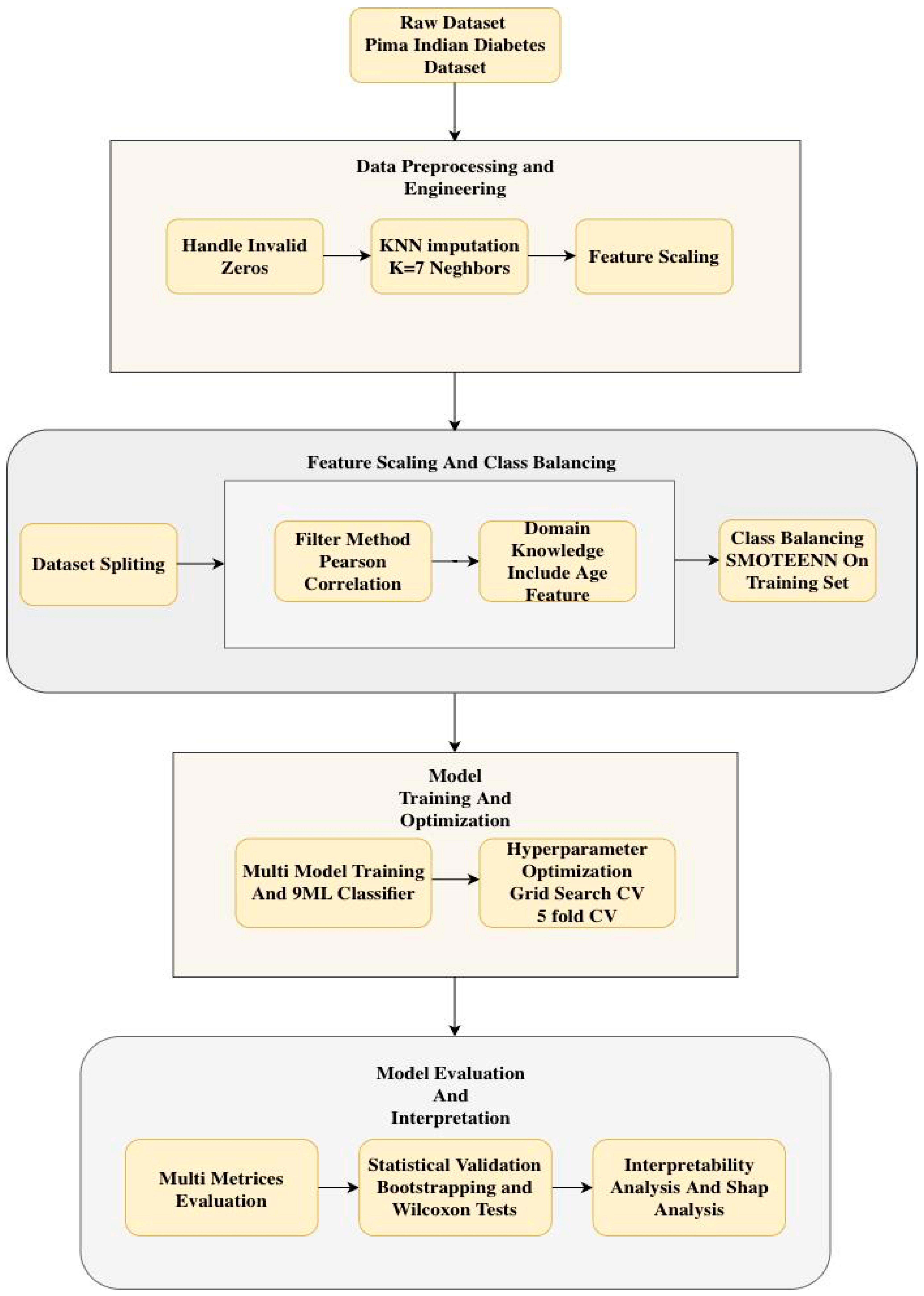
To evaluate and classify diabetic disease, we proposed a three-stage ML model in Python software (version 3.13.2). In order to prepare the dataset for model training in the first stage, we applied data preprocessing and resampling techniques, then in the second stage, we used different classifier ML algorithms for model training and applied a hyperparameter tuning technique. In the last stage, the model evaluation and definition of the explainability aspects of the models are provided. This approach aims to provide a comprehensive analysis and reliable prediction of diabetic disease. The whole pipeline is reported in Figure 1. The full proposed pipeline consisted of three incremental innovations: (1) KNN imputation (k = 7), (2) SMOTEENN hybrid resampling, and (3) our hybrid feature selection method. Each model was evaluated using an identical 5-fold cross-validation scheme on the same data splits to ensure a fair comparison.

2.1. Dataset

This dataset is originally from the National Institute of Diabetes and Digestive and Kidney Diseases, which comprises diagnostic measurements from 768 female patients of Pima Indian heritage. The objective of the dataset is to diagnostically predict whether or not a patient has diabetes, based on certain diagnostic measurements included in the dataset. Several constraints were placed on the selection of these instances from a larger database. In particular, all patients here are females at least 21 years old of Pima Indian heritage. The dataset focuses on a binary class outcome, which classifies patients into two classes including diabetic and non-diabetic. This dataset does not support the multiclass diagnosis of diabetes, including intermediate and pre-diabetic conditions, which are crucial for early diagnosis in the medical field. Table 1 shows the statistics of the input variable.
Figure 1. Diagram of the end-to-end machine learning pipeline for diabetes prediction.
Futureinternet 17 00513 g001
The dataset includes the following eight medical predictor variables and one target variable:
  • Pregnancies: Number of times pregnant.
  • Glucose: Plasma glucose concentration 2 h in an oral glucose tolerance test (mg/dL).
  • BloodPressure: Diastolic blood pressure (mm Hg).
  • SkinThickness: Triceps skin fold thickness (mm), a measure of subcutaneous body fat.
  • Insulin: 2-h serum insulin (mu U/mL).
  • BMI: Body Mass Index (weight in kg/(height in m)2), a measure of body fat based on height and weight.
  • DiabetesPedigreeFunction: A score that indicates the likelihood of diabetes based on family history.
  • Age: Age in years (all patients are at least 21 years old).
  • Outcome: Target variable (0 = no diabetes, 1 = diabetes).
Table 1. Descriptive Statistics of Input Variables.
FeatureDescriptionUnitCountMeanStd DevMin50% (Median)Max
PregnanciesNumber of times pregnant-7683.83.40317
GlucosePlasma glucose concentrationmg/dL768120.932.00117.0199
BloodPressureDiastolic blood pressuremm Hg76869.119.4072.0122
SkinThicknessTriceps skin fold thicknessmm76820.516.0023.099
Insulin2 h serum insulinmu U/mL76879.8115.2030.5846
BMIBody Mass Indexkg/m276832.07.9032.067.1
DiabetesPedigreeFunctionDiabetes likelihood score-7680.50.30.0780.37252.42
AgeAgeYears76833.211.82129.081
OutcomeTarget Variable0 or 17680.350.48001

2.2. Input Variables

The dataset includes eight input features and one binary target variable (Outcome). The input variables considered in this study include Glucose Concentration, Diastolic blood pressure, skin thickness, Insulin, BMI, Age, Diabetes pedigree function, and the output of the proposed model is a class variable with two classes: 0 or 1.

2.3. Data Preprocessing

  • Handling of Invalid Zero Values: The features Glucose, Blood Pressure, Skin Thickness, Insulin, and BMI contained biologically implausible zero values, such as zero blood pressure. These values were treated as missing data (NaN) rather than valid measurements to prevent model bias.
  • KNN Imputation: Missing values were imputed by the KNN Imputation algorithm with 7 neighbors, which provides a balance between using too few neighbors, which can lead to noisy imputations, and too many, which can oversmooth and ignore local patterns. This is the method used over mean or median imputation as it maintains the underlying data distribution and pattern of covariance by filling in missing values based on the similarity of features of the nearest neighbors. Table 2 shows the statistics dataset after KNN imputation.

2.4. Dataset Splitting

Dataset splitting is a core stage for developing robust ML models. Following preprocessing, the dataset was partitioned into two separate subsets, which are the training and testing subsets, to rigorously evaluate model performance and generalizability. An 80-20 split was applied, dedicating 80% of the data for model training and 20% as a hold-out test set for the final evaluation on unknown data [29,30,31]. To achieve a reliable estimate of model performance in development and hyperparameter tuning without using the test set, a 5-Fold Cross-Validation (CV) strategy was applied on the training set in the model development stage.

2.5. Feature Engineering

All features were standardized using StandardScaler, which transforms the data to have a mean of zero and a standard deviation of one. The feature scaling is essential for models that are sensitive to the scale of input features, such as SVM, LR, and KNN. Features were standardized using z-score normalization to ensure comparability across algorithms sensitive to feature scales, such as KNN, SVM algorithms.

2.6. Feature Selection

To avoid overfitting and improve the interpretability of the model, and achieve the best computational cost, the following mixed feature selection method was used:
-
Pearson Correlation Filtering: The absolute value of the correlation coefficient of each feature with the target (Outcome) was calculated. The most correlated features, N = 4, were selected. N = 4 is quantitatively determined by comparison among Pearson correlation coefficients for each of the features and the target variable. The top four features with the highest absolute Pearson correlation to the Outcome were selected: Glucose, BMI, Insulin, and Diabetes Pedigree Function. Based on its established clinical importance, Age was also added to the final set. Thus, the five features used for model development were: Glucose, BMI, Insulin, Diabetes Pedigree Function, and Age.
-
Domain Knowledge Integration: As it had clinically validated relevance, Age was included in the final set of features by design, although it was not among the top N features.

2.7. Handling Class Imbalance

The original dataset is plagued by a class imbalance (approximately 35% diabetic and 65% non-diabetic instances). To combat the associated bias under which models are skewed toward the majority class, a more sophisticated resampling approach was conducted solely on the training set to avoid data leakage.
SMOTEENN: This ensemble algorithm starts by generating synthetic samples from the minority class (SMOTE) and then cleanses the resultant data by removing any misclassified samples by their nearest neighbors (ENN). This hybrid method effectively balances class distribution as well as potentially improves class separability.
This technique goes beyond simple class balancing to actively create a more diverse and robust training environment. It achieves this by enhancing representational diversity in the feature space and sharpening the distinction between classes.
Table 3 shows the statistics of all features before and after class balancing with SMOTEENN.

2.8. Model Development

We chose to use classical machine learning models, specifically tree-based ensembles, for a practical reason since they are well-suited for a dataset like this one. The Pima Indian Diabetes dataset is relatively small and has only a few features. In these cases, well-tuned tree-based models are very effective and less prone to overfitting than deep learning, which usually needs much more data to perform well. Our strong results, which even beat several deep learning models from other studies according to Table 2, confirm that this was the right approach for our study.
Nine ML models were trained for comparison:
  • Ensemble/Boosting: XGBoost, LightGBM, CatBoost, AdaBoost, GB
  • Tree-based: Balanced RF
  • Kernel-based: SVM
  • Distance-based: KNN
  • Linear: LR
The ML approaches adopted in this study are detailed below. The models are chosen based on their ability to handle tabular data and their proven effectiveness in binary classification tasks.
1. SVM: This is a strong classifier that creates a hyperplane in high-dimensional space to separate different classes. By the use of kernel functions, SVM can handle linear and non-linear classification problems. SVM works very well in high-dimensional spaces, but is mostly computationally costly [32].
2. CatBoost: It is a GB algorithm that performs better than other GB algorithms in handling categorical features without extensive preprocessing. It uses ordered boosting to prevent overfitting and make it simple to manage heterogeneous varieties. By combining native categorical variable support with delivery of robust performance with fewer parameters to tune, it is also very accurate on datasets with high levels of categorical have limited features or limited data availability [33].
3. Light GBM: It is a rapid and high-performance GB algorithm. It utilizes a leaf-wise tree growth strategy with depth constraint; consequently, it is more efficient and requires less memory than standard GB. It natively supports large datasets and non-numerical features, making it well-suited for classification problems involving high-dimensional or imbalanced data [34].
4. RF: To enhance accuracy and mitigate overfitting, this ensemble learning technique constructs many DT and combines their outputs. It provides feature relevance scores that facilitate feature selection and performs well on a variety of datasets [35].
5. GB: It is an iterative ensemble learning algorithm that builds predictive models by iteratively adding base learners, most commonly DT, to decrease the residual errors of past models. Every iteration maximizes a loss function according to gradient descent algorithms. It demonstrates high efficacy in classification problems and provides excellent predictive performance, although overfitting must be prevented and generalization achieved through cautious tuning of hyperparameters [36].
6. XGBoost: Using DT as base learners, it is a GB architecture that is both scalable and effective. It is distinguished by its rapid and accurate performance in categorization tasks, particularly when handling unbalanced data [37].
7. AdaBoost: It is an ensemble ML model containing numerous weak learners in a single strong classifier, and it grows sequentially its training models, and the underweight samples receive more weights in each iteration before aggregating their predictions by weighted vote [38].
8. LR: is a supervised ML algorithm used for classification applications. Differing from linear regression, which predicts a range of numbers, it instead predicts the chance that an input is part of a certain group. It works for binary classification, meaning the answer must be one of two options. It uses a sigmoid function to turn any input into a number from 0 to 1 [39].
9. KNN: KNN is a simple, supervised ML algorithm that can be used for classification or regression applications and is also often used in missing value imputation. It is based on the idea that the observations nearest to a given data point are the most similar observations in a dataset, and we can therefore classify unforeseen points according to the values of the closest existing points [40]. The k-NN algorithm classifies all points on the basis of a measure of similarity. The distance between the observations is calculated by using a tree-based data structure. The algorithm predicts the target value for a new data instance by finding the closest data points in the training data as its neighbors. The parameter k is a positive integer representing the number of neighbors to consider. The label of the new instance is classified by majority voting out of these k neighbors. The distance between two points is calculated using Euclidean distance, which measures the straight-line distance in multidimensional space. This is an intuitive and generally accepted measure of similarity in feature space [25].

2.9. Hyperparameter Tuning

We used a systematic approach with 5-fold Stratified Cross-Validation and PR AUC as the optimization metric. RandomizedSearchCV was applied for computationally demanding algorithms (XGBoost, SVM), and GridSearchCV for relatively simpler algorithms. The following Table 4 shows the most significant hyperparameters optimized and their optimized values.
For tree-based models, max_depth and learning_rate parameters were tuned to prevent overfitting and maintain prediction power. For SVM, the regularization parameter C was adjusted to balance margin maximization and classification accuracy. For KNN, n_neighbors was adjusted to balance underfitting and overfitting. This systematic tuning method guaranteed that all algorithms ran at their optimal level and also played a key role in achieving the high-performance rates in our study.

2.10. Model Performance Evaluation

Model performance was compared using a suite of measures selected for their effectiveness, particularly when relevant to imbalanced datasets. The primary model comparison and selection metrics were the Area Under the Receiver Operating Characteristic Curve (ROC-AUC) and the Area Under the Precision-Recall Curve (PR-AUC), which measure the model’s ability to discriminate between classes at any threshold and precision-recall performance on the minority class, respectively. Beyond Youden’s J statistic optimization threshold, we provided precision, recall (sensitivity), F1-score, and balanced accuracy to present the model’s predictive capability in its best operating point. Accuracy quantifies total correctness as the proportion of correct predictions out of total predictions:
Accuracy = (TP + TN)/(TP + TN + FP + FN).
Precision measures prediction quality by determining true positives out of all the positive predictions:
Precision = TP/(TP + FP).
Recall measures completeness as a proportion of correctly identified true positives:
Recall = TP/(TP + FN).
The F1-Score offers a balanced measure through the harmonic mean of Precision and Recall:
F1-Score = 2 × (Precision × Recall)/(Precision + Recall).
Ultimately, the decision of which measure to pursue is not as much of a technical as a strategic one, and one that is largely based on the use and real-world expense of different types of error.

3. Results and Discussion

The performance of nine ML classifiers, which are CatBoost, RF, KNN, LightGBM, XGBoost, SVM, AdaBoost, GB, and LR, was rigorously evaluated on the held-out test set using a comprehensive suite of metrics. The metrics included the Area Under the Receiver Operating Characteristic Curve (ROC AUC), the Area Under the Precision-Recall Curve (PR AUC), Precision, Recall, F1-score, and Accuracy. The results, summarized in Table 5, show that all models reach high performance, with tree-based ensemble methods, particularly CatBoost, having the top performance. The ensemble models performed at the top consistently in the ranks across most of the metrics. CatBoost was the better model and recorded the best results in ROC AUC (0.972), PR AUC (0.972), Recall (0.987), F1-score (0.971), and overall Accuracy (0.968). This indicates that CatBoost provides a great balance between identifying true positive cases (high recall) while maintaining a minimal rate of false positives (high precision), thus making the most potent and strongest predictions overall. The high performance of CatBoost (ROC-AUC: 0.972, Accuracy: 0.968) shows that our end-to-end pipeline successfully addresses key challenges in clinical data, including missing values and class imbalance, while maintaining high predictive power for diabetes detection.
RF followed closely with the second-highest ROC AUC (0.971) and PR AUC (0.972). It registered a higher Precision (0.962) than CatBoost, which is a great testament to its ability to minimize false positives. But its slightly lower Recall compared to CatBoost meant that its F1-score and Accuracy were slightly lower. Notably, the KNN classifier has the best individual value recorded for Precision (0.982). This suggests that if KNN predicts an instance is positive, it will be correct an overwhelmingly large percentage of the time. This was at the cost of lower Recall (0.921), the lowest of the top five, suggesting that it failed to pick up more true positive instances than the top ensembles. The remaining two GB libraries, LightGBM and XGBoost, yielded strong and nearly identical results. SVM also performed well, tying with XGBoost’s Accuracy score (0.953) and showing a high Recall value (0.971), just like CatBoost. The simpler models, AdaBoost, GradientBoost, and LR, trailed the more sophisticated ensembles but were still good. LR, which reported the lowest Accuracy (0.912), had the highest Recall (0.983), bearing witness to its capacity to capture almost all positive instances but at the expense of having a higher proportion of false positives (Precision = 0.872). CatBoost uses a permutation-driven approach to calculate the gradients for each new tree. This results in a more robust and generalizable model, which is critical for smaller clinical datasets where overfitting is a primary concern. CatBoost’s superior algorithm for processing categorical variables makes it inherently robust. It efficiently avoids the overfitting that can occur with simple label encoding, providing a more reliable foundation that benefits all data types. Table 5 shows the results of each algorithm after SMOTEENN. Table 6 shows the evaluation results of each model without the SMOTEENN technique. The results are lower in comparison with Table 5. The performance improvement with SMOTEENN (average F1-score increase from 0.678 to 0.971 for CatBoost) underscores the critical importance of addressing class imbalance in medical datasets, where rare but clinically significant cases must be accurately identified.
Table 5. Result of Evaluation Metrics with SMOTEENN.
ModelROC AUC PR AUC Precision RecallF1 Accuracy
CatBoost0.9720.9720.9560.9870.9710.968
RF0.9710.9720.9620.9540.9580.955
KNN0.9710.9680.9820.9210.9510.948
LightGBM0.9660.9660.9580.9580.9580.955
XGBoost0.9660.9670.9620.9500.9560.953
SVM0.9630.9600.9440.9710.9570.953
AdaBoost0.9620.9640.9420.9420.9420.937
GB0.9610.9620.9460.9420.9440.939
LR0.9510.9550.8720.9830.9240.912
LASSO0.9510.9560.8750.9830.9260.915
Table 6. Result of Evaluation Metrics without SMOTEENN.
ModelROC AUCPR AUCPrecisionRecallF1Accuracy
LR 0.8350.7290.6910.6580.6740.778
GB 0.8250.6880.6130.7850.6880.752
CatBoost 0.8250.6950.5740.8270.6780.726
AdaBoost 0.8220.6890.6120.7380.6690.745
RF 0.8220.6880.5970.7750.6740.739
SVM 0.8110.6830.6480.7660.7020.773
KNN 0.7990.6420.6870.6170.6500.768
LightGBM 0.7950.6490.6030.7470.6680.741
XGBoost 0.7750.6480.5780.7430.6500.721
Table 7 is a comparative performance analysis of our proposed methodology compared to existing state-of-the-art in diabetes prediction. Our CatBoost model performs best on all the evaluation metrics, with the highest ROC-AUC (0.972), accuracy (0.968), and F1-score (0.971). The model performs very well in precision (0.956) and recall (0.987) as well, which indicates excellent performance in the identification of true positive cases while maintaining a minimum of false positives.
Table 8 shows the performance of the catboost algorithm on different K imputations with the different values, including k = 4, 6, 7, 8. At K = 4, the model achieves very high recall, successfully identifying nearly all positive instances, but creates more false-positive errors (worse precision). At K = 6, as opposed to this becomes too simplistic and shows signs of underfitting, as it has worse recall and accuracy measures. The best performance is achieved at K = 7, where sensitivity and precision are in a good balance, obtaining the highest values among all K. Finally, at K = 8 confirms that the optimum has been exceeded because its performance begins a slow but continuous decline, so it shows good performance but not maximum.

3.1. Feature Correlation Analysis

We used a Pearson correlation matrix to identify linear relationships between all possible pairs of variables. It creates a symmetric matrix in which each cell holds a coefficient ranging from −1 to +1 that defines the strength and direction of each linear relationship. The correlation matrix identified strong linear relationships between the predictive features and the target variable. According to the coefficient matrix in Figure 2, Glucose is strongly positively correlated with Insulin (r = 0.64) and the Outcome (r = 0.50), indicating its role as a key predictor, which means that higher blood glucose levels typically trigger the release of more insulin. This is a fundamental biological relationship. Insulin was strongly positively correlated with Glucose and moderately correlated with BMI (r = 0.32). Strong correlation was observed between BMI and Skin Thickness (r = 0.64). Skin thickness was weakly to moderately correlated with Metabolic parameters such as Insulin (r = 0.25) and Glucose (r = 0.24). Age had the weakest correlation among all the features, and it correlated most strongly with Outcome (r = 0.24). Outcome was most strongly influenced by Glucose, then Insulin and BMI. These correlations not only agree with the available clinical knowledge but also justify the incorporation of these variables in the subsequent ML models to make a prediction regarding the outcome.

3.2. Model Robustness: Cross-Validation ROC Analysis

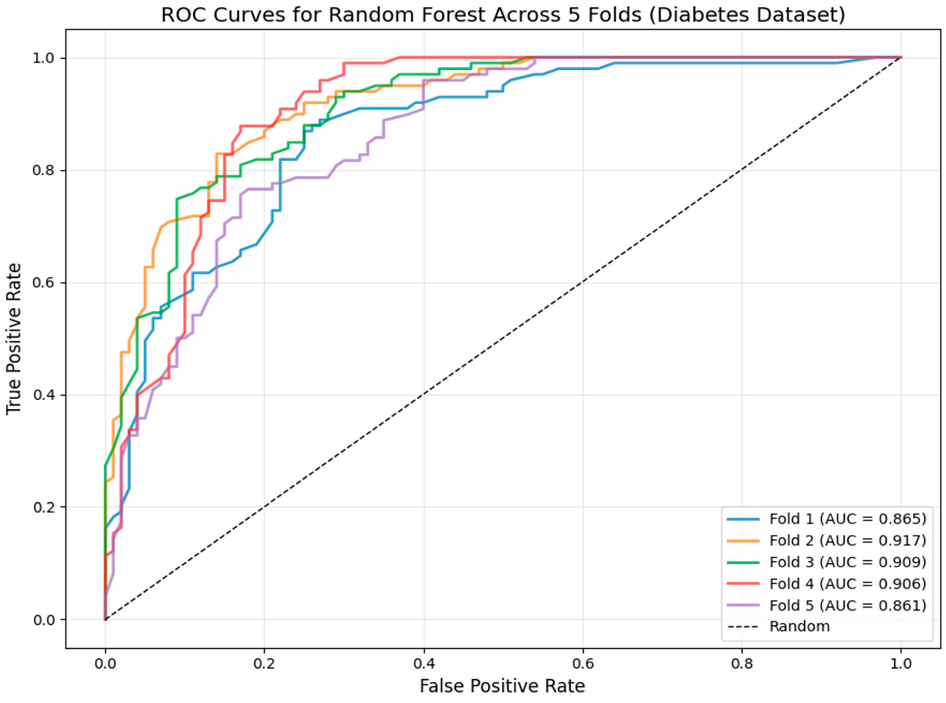
In order to confirm the stability and robustness of the model, we cross-checked its performance on over one validation fold. Figure 3 displays the ROC curves of the Random Forest classifier for all five folds with remarkably consistent results, with AUC values between 0.861 and 0.917. The tight clustering of these curves shows low variance, proving the discrimination power of the model between diabetic and non-diabetic patients is robust and does not depend on some particular subset of the data. This consistency gives us high confidence that the model will perform well with new data. The dashed line representing a random classifier (AUC = 0.5) serves as a baseline for comparison.

3.3. Feature Importance and Impact via SHAP Analysis

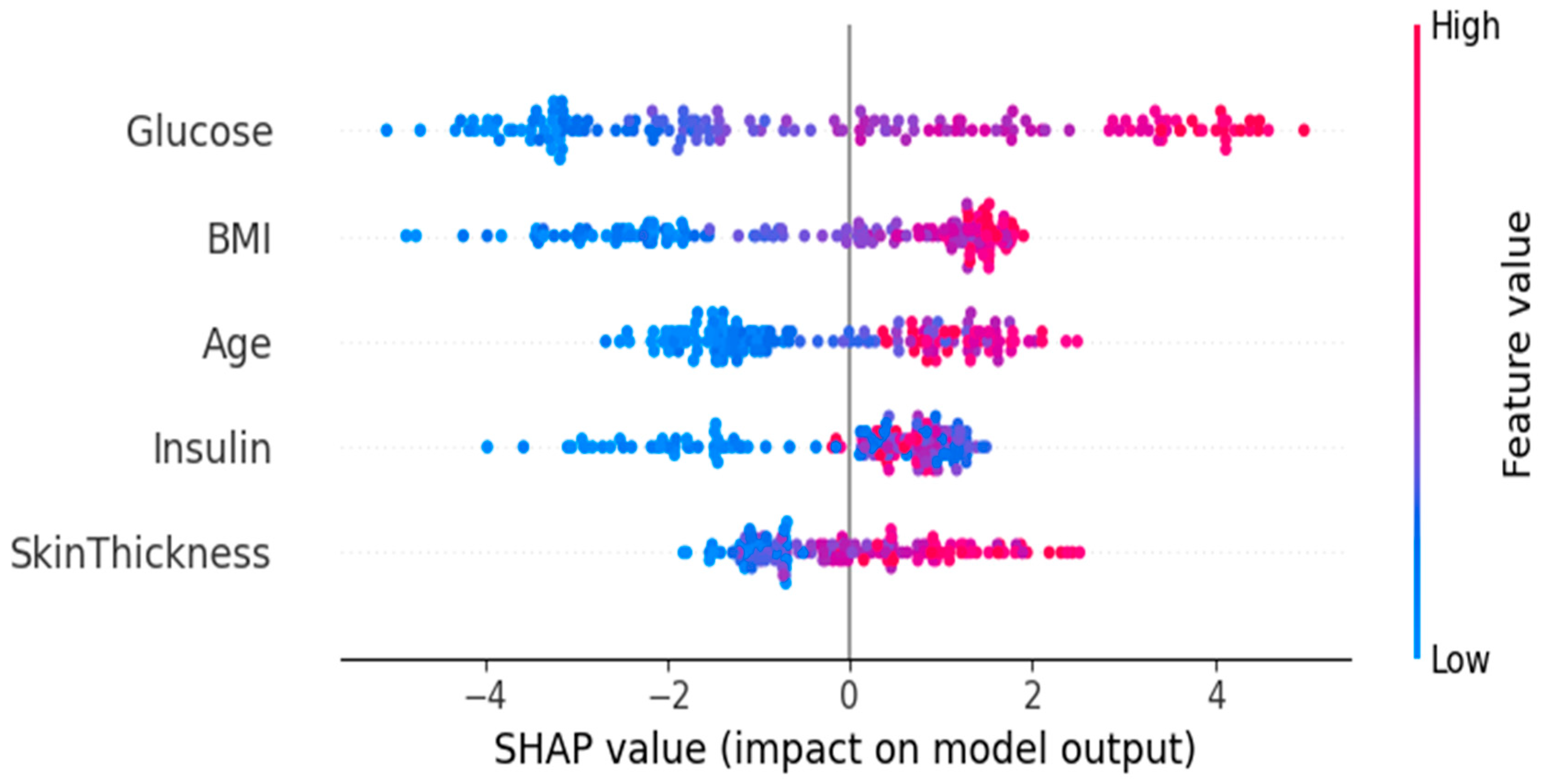
The SHAP summary plot in Figure 4 gives an idea of how relevant each feature and direction of influence is to the model’s output by the top predictors. The horizontal axis represents the SHAP value, which quantifies each feature’s impact on the model’s final prediction; values greater than zero increase the prediction score, which raises the estimated risk of diabetes, while values less than zero decrease it. The plot lists the clinical features, including Glucose, BMI, Age, Insulin, and SkinThickness on the vertical axis, ranked from top to bottom by their overall importance. The horizontal spread of SHAP values indicates the magnitude of a feature’s impact. A wider range, as seen with glucose, shows it has a larger influence on the final risk prediction than features with a narrower spread, such as SkinThickness. The most dominant feature was Glucose, where a clear trend shows that higher values (red) are strongly associated with a positive model output (increased risk), while lower values (blue) are strongly associated with a negative output (decreased risk). BMI and Age also produced high positive effects, with high values causing an increase in the model’s output. Insulin showed a definite deviation, with extremely high and extremely low values having large but opposing effects on prediction. Skin Thickness, while less intimidating, showed a pattern where higher values slightly boosted the predicted result. The plot as a whole confirms the finding that clinically significant variables drive the model’s outcome, with bi-directional effects plainly apparent for major metabolic characteristics. SHAP explainability is at the heart of patient engagement. Instead of a black-box prediction, a Clinical Decision Support System would be able to return to both the patient and the physician a visual explanation. The output of the model can also be a helpful triage tool. An automatically flagged high-glucose, high-BMI patient would be considered high-risk and hence in need of urgent and more comprehensive diagnostic tests. The model output can be used as an effective triage tool. In a live clinical setting, the model can be incorporated into a Decision Support System and utilized to stratify patient risk. A Glucose high and BMI high patient would automatically be high-risk tagged and prompt immediate and enhanced diagnostic testing, such as HbA1c, oral glucose tolerance test. Conversely, a low-risk prediction for a patient with borderline values in a single attribute will warrant a wait-and-see approach and advice concerning lifestyle issues, optimizing the use of resources. This changes the model from one of prediction to one of triage and clinical judgment facilitation. The consistency of SHAP analysis and univariate statistical tests with one another provides corroborative evidence that our model learns medically meaningful patterns and not spurious correlations, inspiring confidence in clinical deployment.
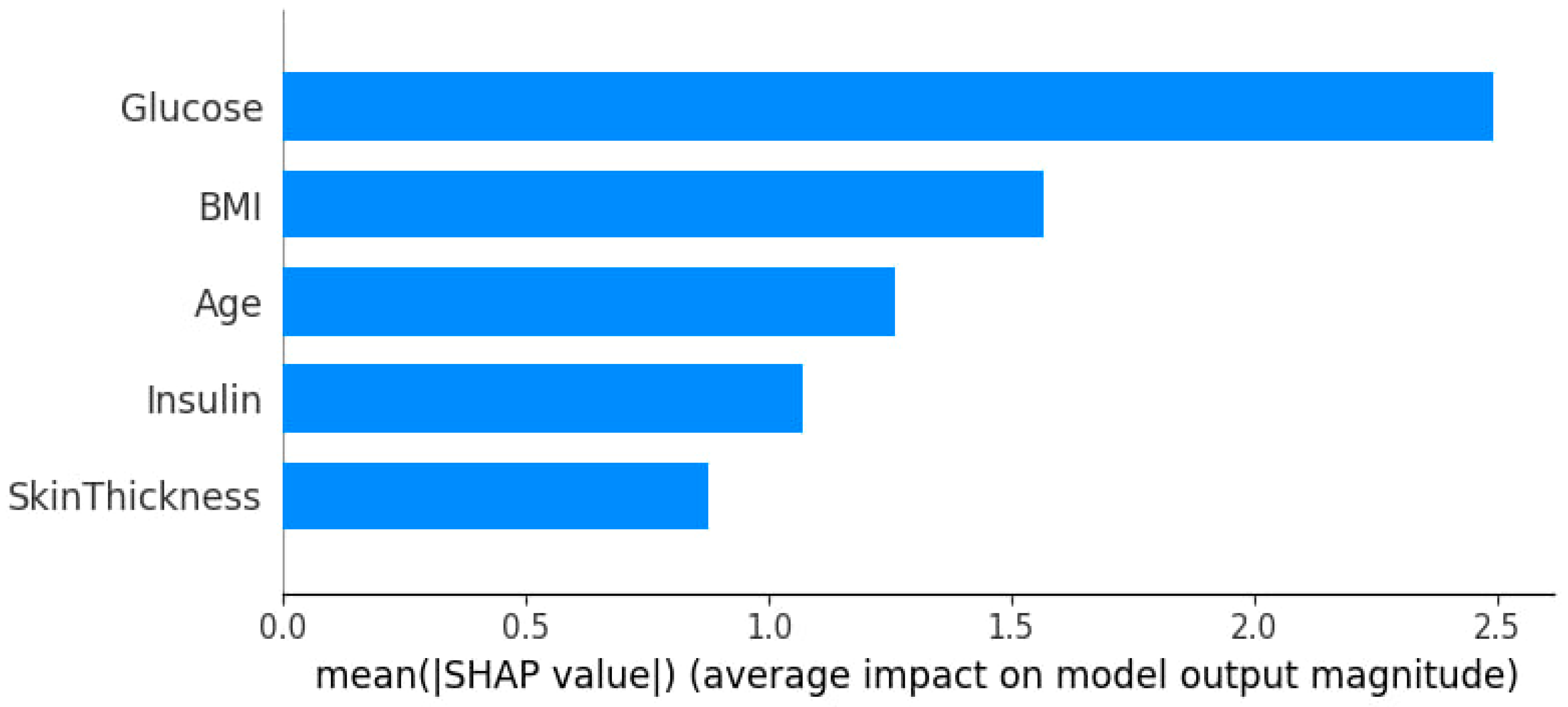
Figure 5 shows the average impact of each feature on the model output based on the mean SHAP value. This plot quantitatively summarizes the overall importance of the top features. Based on the provided SHAP summary plot, the most important feature for the model to make its prediction is Glucose, followed by BMI and Age. Insulin and Skin Thickness contribute comparatively less towards the outcome of the model. The ranking is consistent with the patterns observed in the SHAP summary plot according to Figure 4 and the univariate analysis based on Table 9, reinforcing their clinical validity. This indicates that the metabolic factors are influencing the model’s decision-making process the most. This figure presents a clear evidence-based plan for clinicians to establish blood glucose management and BMI control early and first-line measures to prevent and detect diabetes early.

3.4. Univariate Analysis of Feature Associations with Diabetes

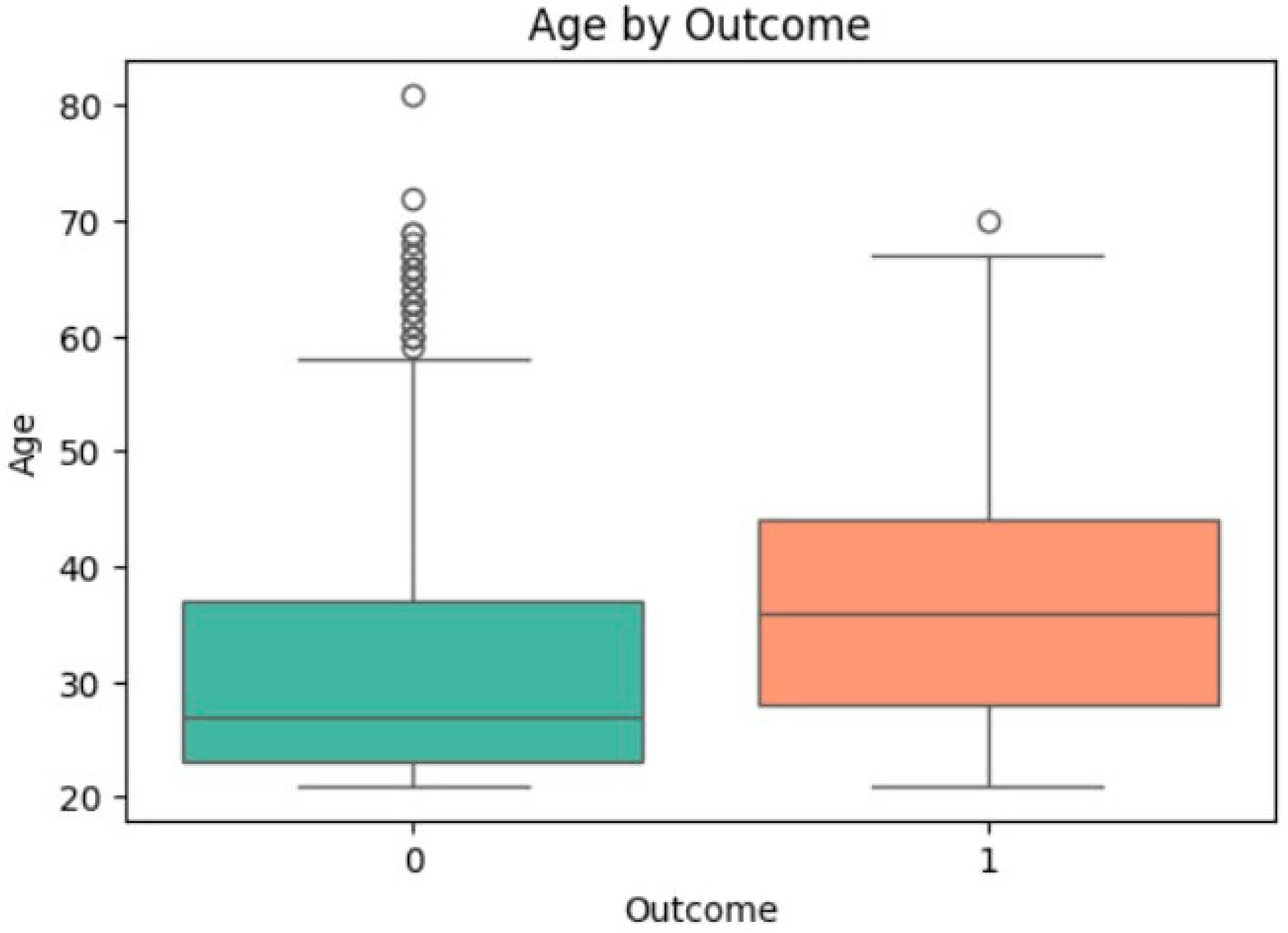
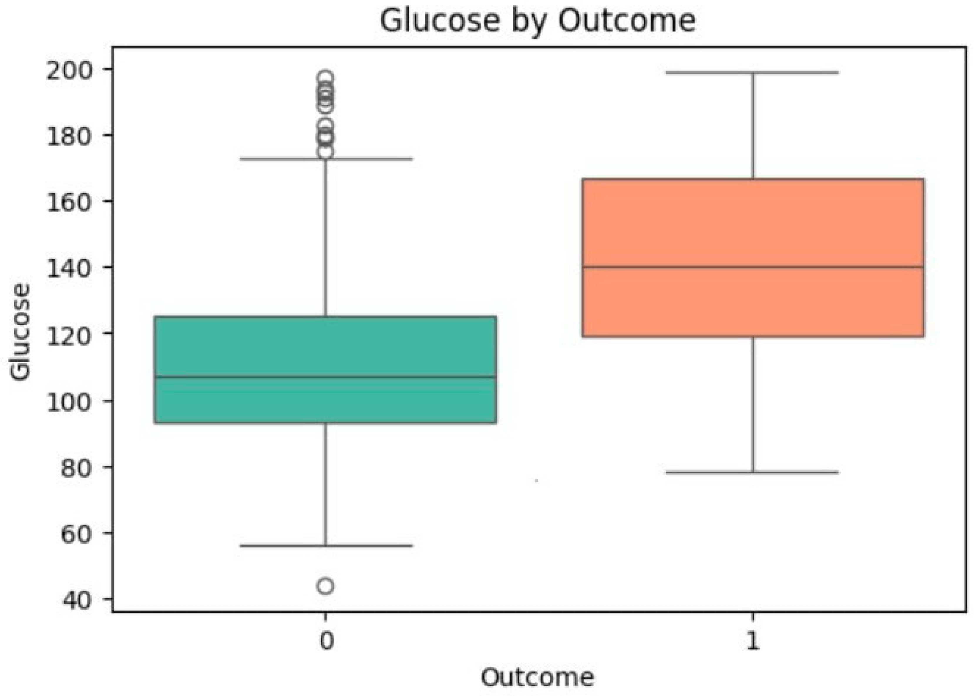
We used a univariate analysis for each selected feature by t-tests and logistic regression. For Age, the logistic coefficient is 0.042 (OR = 1.043), which means that each year increases diabetes odds by ~4.3% according to Figure 6. The box plot shows that the median age for the diabetic group (Outcome = 1) is higher than for the non-diabetic group (Outcome = 0) and shows a strong relation between age and diabetes. For Glucose, the coefficient is 0.041 (OR = 1.042), meaning each 1 mg/dL increase raises diabetes odds by ~4.2% according to Figure 7. Similar significant effects were observed for Insulin, BMI, and SkinThickness. These results confirm the clinical relevance of the features and complement the SHAP analysis by quantifying individual impacts.
The results of the univariate analysis are detailed in Table 9. All features showed significantly higher values in diabetic patients (p < 0.0001), as evidenced by the consistently negative T-statistics. Glucose demonstrated the strongest overall association (Cohen’s d = 1.195; t = −14.97), indicating it is the most powerful discriminator between groups. Notably, BMI showed the highest diabetes risk per unit increase (OR = 1.109). The large magnitude of these statistics reflects a strong separation between the diabetic and non-diabetic cohorts. These results do more than just validate statistical significance; they validate the clinical logic of the model. By establishing that the model’s key features are precisely those with the strongest independent epidemiological relationships to diabetes, we build a bridge of trust between the algorithm’s inner workings and a physician’s expert knowledge. This strong, statistically validated foundation of feature associations provides a principled explanation for the high predictive performance achieved by the ensemble models, particularly CatBoost. This statistical validation confirms what the SHAP analysis revealed: Glucose and BMI are the most critical factors. When both traditional statistics and modern explainable AI point to the same risk factors, it gives us confidence that the model is making decisions for the right reasons using medically sound logic that doctors can understand and trust.
Table 9. Univariate Analysis of Predictor Variables.
FeatureT-Statisticp-Value (t-test)Mean (Group 0)Mean (Group 1)Cohen’s dOdds Ratio (OR)0.95 CI for ORp-Value (Regression)
Glucose −14.974<0.0001110.57142.241.1951.042[1.035, 1.049]<0.0001
Insulin −8.851<0.0001129.89195.290.7121.008[1.006, 1.010]<0.0001
BMI −9.097<0.000130.8535.380.6921.109[1.082, 1.136]<0.0001
SkinThickness −8.037<0.000127.1932.610.6071.072[1.052, 1.092]<0.0001
Age −6.921<0.000131.1937.070.5141.043[1.030, 1.056]<0.0001
The negative T-statistics in Table 9 indicate that the mean values of all clinical features are significantly higher in the diabetic group (Outcome = 1) compared to the non-diabetic group (Outcome = 0). This directional relationship is consistent across all predictors: Glucose, Insulin, BMI, Skin Thickness, and Age all show substantially elevated levels in diabetic patients. The large magnitude of these T-statistics, particularly for Glucose (t = −14.974), reflects strong separation between the groups and confirms that diabetic patients present with clinically elevated metabolic parameters.

3.5. Comparative Model Performance and Statistical Validation

Table 10 shows the comparative model performance and statistical validation. All models demonstrated strong predictive performance, with ROC AUC scores exceeding 0.95 and F1-scores ranging from 0.925 to 0.971. CatBoost achieved the highest F1-score (0.971, 0.95 CI [0.955–0.984]) and Accuracy (0.968, 0.95 CI [0.953–0.984). However, other ensemble models, including Random Forest, LightGBM, XGBoost, and SVM, also delivered comparable and stable results. To evaluate statistical significance, we performed Wilcoxon signed-rank tests for fold-level F1-scores. Bootstrapping (1000 resamples, 0.95 CI) was performed for Confidence intervals of Accuracy, F1, and ROC AUC, and shows the reproducibility and stability of the introduced method.

3.6. Clinical Translation and Actionable Insights

While SHAP analysis provides fascinating information on feature importance, this must be framed in useful clinical advice. The significant contributions of Glucose, BMI, and Age to predictions underscore the need for targeted screening and prevention in patients who have elevated values for these variables. Physicians can leverage these observations to stratify the subgroup at risk for earlier and more aggressive surveillance, counseling, or drug therapy. Also, a bidirectional Insulin effect where low and high values both contribute to predictions would suggest the need for careful clinical assessment, possibly indicative of insulin resistance or beta-cell dysfunction. SHAP-based explanations integrated into clinical decision support would enable personalized risk visualizations to help clinicians facilitate more intuitive risk communication and engage patients more actively in their management. Our results support the integration of an interpretable clinical workflow. When our model identifies a high-risk patient, the accompanying SHAP explanation clarifies the contributing factors. In the high-risk case, a prediction driven primarily by Glucose >140 mg/dL and BMI >30 could show an immediate referral for confirmatory HbA1c testing and lifestyle intervention. Conversely, low-risk predictions for borderline cases might justify routine monitoring, optimizing resource allocation. SHAP analysis for interpretability of our model bridges the gap between clinical judgment between algorithmic predictions and clinical judgment. Unlike black-box models that only provide a risk score, our approach offers transparent, factor-by-factor explanations that clinicians can review and validate against their medical expertise. Such transparency is important to ensure credibility as well as to allow AI tools to be integrated into routine clinical practice.

3.7. Multi-Dataset Generalizability Assessment

One of the major goals of this manuscript is to assess the generalizability of predictive models beyond the constraints of a single dataset. While useful for benchmarking, the Pima Indians Diabetes Dataset has few sample sizes, n = 768, and a narrow demographic scope, which calls for validation in a larger and more diverse population. We further validated model performance on two additional large datasets to ensure performance and clinical applicability. This manuscript was expanded to include a larger and more diverse clinical dataset.

3.7.1. Validation Dataset 1: CDC BRFSS 2015 Dataset

We used the CDC BRFSS 2015 dataset, which consists of 253,680 survey responses from the Kaggle website. This large dataset improves the performance and scientific contribution of our work by using different models and several patient populations. We employed nine machine learning models, and the results are summarized in Table 11. The results show that the advanced gradient-boosting ensembles are based on exceptionally high performance. CatBoost and XGBoost showed the high-performing models; they achieved an accuracy of 0.91 and a robust ROC AUC of 0.967. This result shows that the strong power of these models is not an artifact of a single, small dataset but is generalizable to a wide range of clinical contexts.

3.7.2. Validation Dataset 2: Diabetes 130-US Hospitals Dataset

This dataset includes 10 years of clinical data (from 1999 to 2008, n = 101,766) provided from 130 US hospitals and is available on the Kaggle website. According to the performance comparison in Table 12, tree-based boosting algorithms such as LightGBM, XGBoost, and CatBoost achieved the best performance and showed highly similar and superior results in almost all metrics, with accuracy above 0.93 and an F1 score of around 0.93. These three models perform especially well on precision, ranging between 0.987 and 0.994, which means their positive predictions are always close to correct, while a value of 0.87 for recall means a slight trade-off: they miss roughly 13% of the actual positive instances. On the other hand, the random forest model yields a decent performance but noticeably lower, with an accuracy of 0.865 and an F1-score of 0.862. The Logistic Regression model is far behind them, with all its metrics around 0.60, which indicates that it is poorly suited for the task at hand due to failure to capture the underlying nonlinear relationships in the data.

3.7.3. Cross-Dataset Performance Consistency

We summarize the cross-dataset robustness of the proposed methodology with the performance of the top three ensemble algorithms across all three datasets in Table 13. Results show high performance, regardless of dataset size or demographic composition. CatBoost, XGBoost, and LightGBM maintain strong results on every metric. This result, particularly the high ROC AUC exceeding 0.95, balanced Precision-Recall values, and consistent accuracy above 0.90, demonstrates the generalizability and reliability of the end-to-end pipeline, which we developed for predicting diabetes in diverse clinical and population health contexts.

4. Conclusions

This research efficiently developed a robust and interpretable machine learning pipeline for diabetic disease early detection. Among the models, CatBoost generated the most effective algorithm with an ROC-AUC of 0.972 and an accuracy of 0.968. SHAP analysis validated the most significant predictors of factors to be glucose, BMI, and age, findings that were also upheld by univariate analysis, in which Glucose had the highest correlation (Cohen’s d = 1.195) and BMI had the highest diabetes risk for every unit increase (OR = 1.109). The combination of SHAP with traditional statistical validation brings multiple levels of interpretability, while SHAP opens the black box of the model’s decision process to each prediction. Univariate analysis confirms such findings through standard statistical procedures. This two-component approach ensures that our model is not only precise but clinically interpretable and actionable as well.
Blending functionally novel missing data handling (KNN imputation) and class imbalance (SMOTEENN) was critical to developing a method that will achieve high accuracy and clinical interpretability. The findings offer a reasonable reason for employing Gradient-Boosted Trees (GBTs) in this role. For our specific project, which involved a classic, structured tabular dataset of a limited size, the balance of trade-offs strongly favored GBTs. For tabular data structured in this quantity, GBTs offer a superior balance in performance, lower cost of computation, and high interpretability to more advanced deep learning that most frequently require larger datasets in order to operate at their best, and that often serve as black boxes. Deep learning truly shines with very large datasets or multi-modal data, which combines images with tabular data, where its capacity for learning complex representations can be fully leveraged. For our project’s context, the computational and data requirements of deep learning were not justified, and the trade-offs unequivocally favored GBTs [44,45].
As a whole, this study not only provides a highly precise model for forecasting diabetes but also brings a data-driven, reproducible method applicable to intelligent healthcare systems. The pipeline architecture, based on a practically implemented and high-performance modeling approach, is consistent with the requirement of future Internet-of-Things-based clinical decision-making support, for which explainable and actionable knowledge is required [46].
This robustness of the pipeline is established across three datasets, including the Pima Indian dataset, the large-scale CDC BRFSS 2015 dataset, and the clinical Diabetes 130-US hospitals records. This multi-dataset evaluation establishes that our methodology generalizes effectively beyond a single, limited group of individuals into diverse demographic and clinical environments. The strong performance of our pipeline, consistently achieving accuracy above 0.90 and ROC AUC above 0.95 across three distinct datasets, including Pima Indian, CDC BRFSS 2015, and Diabetes 130-US Hospitals, provides robust evidence for its generalizability. This multi-source validation is a crucial step towards the reliable integration of such AI tools in diverse and real-world clinical environments.
This study has several limitations. First, the dataset, while standard, is relatively small and homogenous, which may limit the generalizability of the model to other populations. Second, the features are limited to clinical measurements; incorporating more diverse data types, including genetic markers, lifestyle data, and continuous glucose monitoring data, could improve predictive power.
Future research directions include:
  • External Validation: using larger, multi-ethnic, and more recent datasets to validate robustness and generalizability.
  • Multi-Modal Data Integration: developing the model by integrating other data types, such as medical images or textual data.
  • Real-Time Deployment: Implementing a real-time web service or mobile application within an IoT-enabled healthcare framework.
  • Advanced Explainability: Using other explainable AI methods to provide case-based explanations for clinicians.

Author Contributions

Conceptualization, Y.B., A.B., F.B., F.D., I.G. and P.P.; Methodology, Y.B. and A.B.; Software, Y.B. and A.B.; Validation, Y.B. and A.B.; Funding Acquisition, Y.B.; Formal Analysis, Y.B. and A.B.; Investigation, Y.B. and A.B.; Resources, Y.B., F.B. and F.D.; Data Curation, Y.B. and A.B; Writing—Original Draft Preparation, Y.B. and A.B.; Writing—Review and Editing, Y.B., A.B., F.B., F.D., I.G. and P.P.; Visualization, Y.B. and A.B.; Supervision, F.B. and F.D.; Project Administration, F.B. and F.D. funding acquisition, Y.B. All authors have read and agreed to the published version of the manuscript.

Funding

One of the authors of the manuscript (Yas Barzegar) holds a Ph.D. scholarship funded by Unidata S.p.A. (CUP-B53C22003700004) and the National Recovery and Resilience Plan of Italy (PNRR) (38-033-26-DOT1326HYC-3052).

Institutional Review Board Statement

Not applicable.

Informed Consent Statement

Not applicable.

Data Availability Statement

Publicly available datasets were analyzed in this study. This data can be found here: (https://www.kaggle.com/datasets/vaibhavgovindwar/pima-indian-diabetes, accessed on 30 August 2025).

Conflicts of Interest

Author Patrizio Pisani was employed by the company S.p.A. The remaining authors declare that the research was conducted in the absence of any commercial or financial relationships that could be construed as a potential conflict of interest.

References

  1. Ahmed, Z.; Mohamed, K.; Zeeshan, S.; Dong, X. Artificial intelligence with a multi-functional machine learning platform development for better healthcare and precision medicine. Database 2020, 2020, baaa010. [Google Scholar] [CrossRef]
  2. Caballé-Cervigón, N.; Castillo-Sequera, J.L.; Gómez-Pulido, J.A.; Gómez-Pulido, J.M.; Polo-Luque, M.L. Machine learning applied to diagnosis of human diseases: A systematic review. Appl. Sci. 2020, 10, 5135. [Google Scholar] [CrossRef]
  3. Standl, E.; Khunti, K.; Hansen, T.B.; Schnell, O. The global epidemics of diabetes in the 21st century: Current situation and perspectives. Eur. J. Prev. Cardiol. 2019, 26, 7–14. [Google Scholar] [CrossRef] [PubMed]
  4. Behera, B.; Irshad, A.; Rida, I.; Shabaz, M. AI-driven predictive modeling for disease prevention and early detection. SLAS Technol. 2025, 31, 100263. [Google Scholar] [CrossRef]
  5. Chae, S.; Kwon, S.; Lee, D. Predicting Infectious Disease Using Deep Learning and Big Data. Int. J. Environ. Res. Public Health 2018, 15, 1596. [Google Scholar] [CrossRef]
  6. Nilashi, M.; Asadi, S.; Abumalloh, R.A.; Samad, S.; Ghabban, F.; Supriyanto, E.; Osman, R. Sustainability performance assessment using self-organizing maps (SOM) and classification and ensembles of regression trees (CART). Sustainability 2021, 13, 3870. [Google Scholar] [CrossRef]
  7. Bhatt, C.M.; Patel, P.; Ghetia, T.; Mazzeo, P.L. Effective heart disease prediction using machine learning techniques. Algorithms 2023, 16, 88. [Google Scholar] [CrossRef]
  8. Islam, M.M.; Haque, M.R.; Iqbal, H.; Hasan, M.M.; Hasan, M.; Kabir, M.N. Breast cancer prediction: A comparative study using machine learning techniques. SN Comput. Sci. 2020, 1, 290. [Google Scholar] [CrossRef]
  9. Sakib, S.; Tanzeem, A.K.; Tasawar, I.K.; Shorna, F.; Siddique, M.A.B.; Alam, S.B. Blood cancer recognition based on discriminant gene expressions: A comparative analysis of optimized machine learning algorithms. In Proceedings of the 2021 IEEE 12th Annual Information Technology, Electronics and Mobile Communication Conference (IEMCON), Vancouver, BC, Canada, 27–30 October 2021; IEEE: Piscataway, NJ, USA, 2021; pp. 0385–0391. [Google Scholar]
  10. Al Reshan, M.S.; Amin, S.; Zeb, M.A.; Sulaiman, A.; Alshahrani, H.; Shaikh, A. A robust heart disease prediction system using hybrid deep neural networks. IEEE Access 2023, 11, 121574–121591. [Google Scholar] [CrossRef]
  11. Nandy, S.; Adhikari, M.; Balasubramanian, V.; Menon, V.G.; Li, X.; Zakarya, M. An intelligent heart disease prediction system based on swarm-artificial neural network. Neural Comput. Appl. 2023, 35, 14723–14737. [Google Scholar] [CrossRef]
  12. Ghaffar Nia, N.; Kaplanoglu, E.; Nasab, A. Evaluation of artificial intelligence techniques in disease diagnosis and prediction. Discov. Artif. Intell. 2023, 3, 5. [Google Scholar] [CrossRef] [PubMed]
  13. Kor, C.-T.; Li, Y.-R.; Lin, P.-R.; Lin, S.-H.; Wang, B.-Y.; Lin, C.-H. Explainable Machine Learning Model for Predicting First-Time Acute Exacerbation in Patients with Chronic Obstructive Pulmonary Disease. J. Pers. Med. 2022, 12, 228. [Google Scholar] [CrossRef] [PubMed]
  14. Alex, S.A.; Nayahi, J.J.V.; Shine, H.; Gopirekha, V. Deep convolutional neural network for diabetes mellitus prediction. Neural Comput. Appl. 2022, 34, 1319–1327. [Google Scholar] [CrossRef]
  15. El-Jerjawi, N.S.; Abu-Naser, S.S. Diabetes prediction using artificial neural network. Int. J. Adv. Sci. Technol. 2018, 121, 54–64. [Google Scholar]
  16. El-Bashbishy, A.E.S.; El-Bakry, H.M. Pediatric diabetes prediction using deep learning. Sci. Rep. 2024, 14, 4206. [Google Scholar] [CrossRef]
  17. Wei, S.; Zhao, X.; Miao, C. A comprehensive exploration to the machine learning techniques for diabetes identification. In Proceedings of the 2018 IEEE 4th World Forum on Internet of Things (WF-IoT), Singapore, 5–8 February 2018; IEEE: Piscataway, NJ, USA, 2018; pp. 291–295. [Google Scholar]
  18. Chandgude, N.; Pawar, S. Diagnosis of diabetes using Fuzzy inference System. In Proceedings of the 2016 International Conference on Computing Communication Control and Automation (ICCUBEA), Pune, India, 12–13 August 2016; pp. 1–6. [Google Scholar] [CrossRef]
  19. Barzegar, Y.; Gorelova, I.; Bellini, F.; D’ascenzo, F. Drinking water quality assessment using a fuzzy inference system method: A case study of Rome (Italy). Int. J. Environ. Res. Public Health 2023, 20, 6522. [Google Scholar] [CrossRef] [PubMed]
  20. Barzegar, Y.; Barzegar, A.; Bellini, F.; Marrone, S.; Verde, L. Fuzzy inference system for risk assessment of wheat flour product manufacturing systems. Procedia Comput. Sci. 2024, 246, 4431–4440. [Google Scholar] [CrossRef]
  21. Bellini, F.; Barzegar, Y.; Barzegar, A.; Marrone, S.; Verde, L.; Pisani, P. Sustainable water quality evaluation based on cohesive Mamdani and Sugeno fuzzy inference system in Tivoli (Italy). Sustainability 2025, 17, 579. [Google Scholar] [CrossRef]
  22. Barzegar, Y.; Barzegar, A.; Marrone, S.; Verde, L.; Bellini, F.; Pisani, P. Computational Risk Assessment in Water Distribution Network. In International Conference on Computational Science; Springer Nature: Cham, Switzerland, 2025; pp. 167–174. [Google Scholar]
  23. Barzegar, A.; Campanile, L.; Marrone, S.; Marulli, F.; Verde, L.; Mastroianni, M. Fuzzy-based severity evaluation in privacy problems: An application to healthcare. In Proceedings of the 2024 19th European Dependable Computing Conference (EDCC), Leuven, Belgium, 8–11 April 2024; IEEE: Piscataway, NJ, USA, 2024; pp. 147–154. [Google Scholar]
  24. Naseem, A.; Habib, R.; Naz, T.; Atif, M.; Arif, M.; Allaoua Chelloug, S. Novel Internet of Things based approach toward diabetes prediction using deep learning models. Front. Public Health 2022, 10, 914106. [Google Scholar] [CrossRef]
  25. Verma, N.; Singh, S.; Prasad, D. Machine learning and IoT-based model for patient monitoring and early prediction of diabetes. Concurr. Comput. Pract. Exp. 2022, 34, e7219. [Google Scholar] [CrossRef]
  26. Cong, Z.; Luo, X.; Pei, J.; Zhu, F.; Zhang, Y. Data pricing in machine learning pipelines. Knowl. Inf. Syst. 2022, 64, 1417–1455. [Google Scholar] [CrossRef]
  27. Mohr, F.; Wever, M.; Tornede, A.; Hüllermeier, E. Predicting machine learning pipeline runtimes in the context of automated machine learning. IEEE Trans. Pattern Anal. Mach. Intell. 2021, 43, 3055–3066. [Google Scholar] [CrossRef]
  28. Olson, R.S.; Moore, J.H. TPOT: A tree-based pipeline optimization tool for automating machine learning. In Proceedings of the Workshop on Automatic Machine Learning, New York, NY, USA, 24 June 2016; PMLR: London, UK, 2016; pp. 66–74. [Google Scholar]
  29. Baccouche, A.; Garcia-Zapirain, B.; Castillo Olea, C.; Elmaghraby, A. Ensemble deep learning models for heart disease classification: A case study from Mexico. Information 2020, 11, 207. [Google Scholar] [CrossRef]
  30. Chandra, J.B.; Nasien, D. Application of machine learning k-nearest neighbour algorithm to predict diabetes. Int. J. Electr. Energy Power Syst. Eng. 2023, 6, 134–139. [Google Scholar] [CrossRef]
  31. Korkmaz, A.; Bulut, S. Machine learning for early diabetes screening: A comparative study of algorithmic approaches. Serbian J. Electr. Eng. 2025, 22, 93–112. [Google Scholar] [CrossRef]
  32. Rezvani, S.; Pourpanah, F.; Lim, C.P.; Wu, Q.M. Methods for class-imbalanced learning with support vector machines: A review and an empirical evaluation. arXiv 2024, arXiv:2406.03398. [Google Scholar] [CrossRef]
  33. Hancock, J.T.; Khoshgoftaar, T.M. CatBoost for big data: An interdisciplinary review. J. Big Data 2020, 7, 94. [Google Scholar] [CrossRef]
  34. Lokker, C.; Abdelkader, W.; Bagheri, E.; Parrish, R.; Cotoi, C.; Navarro, T.; Germini, F.; Linkins, L.A.; Haynes, R.B.; Chu, L.; et al. Boosting efficiency in a clinical literature surveillance system with LightGBM. PLOS Digit. Health 2024, 3, e0000299. [Google Scholar] [CrossRef]
  35. Parmar, A.; Katariya, R.; Patel, V. A review on random forest: An ensemble classifier. In International Conference on Intelligent Data Communication Technologies and Internet of Things; Springer International Publishing: Cham, Switzerland, 2018; pp. 758–763. [Google Scholar]
  36. Theerthagiri, P.; Vidya, J. Cardiovascular disease prediction using recursive feature elimination and gradient boosting classification techniques. Expert Syst. 2022, 39, e13064. [Google Scholar] [CrossRef]
  37. Budholiya, K.; Shrivastava, S.K.; Sharma, V. An optimized XGBoost based diagnostic system for effective prediction of heart disease. J. King Saud Univ.-Comput. Inf. Sci. 2022, 34, 4514–4523. [Google Scholar] [CrossRef]
  38. Asra, T.; Setiadi, A.; Safudin, M.; Lestari, E.W.; Hardi, N.; Alamsyah, D.P. Implementation of AdaBoost algorithm in prediction of chronic kidney disease. In Proceedings of the 2021 7th International Conference on Engineering, Applied Sciences and Technology (ICEAST), Pattaya, Thailand, 1–3 April 2021; IEEE: Piscataway, NJ, USA, 2021; pp. 264–268. [Google Scholar]
  39. Ciu, T.; Oetama, R.S. Logistic regression prediction model for cardiovascular disease. IJNMT (Int. J. New Media Technol.) 2020, 7, 33–38. [Google Scholar] [CrossRef]
  40. Uddin, S.; Haque, I.; Lu, H.; Moni, M.A.; Gide, E. Comparative performance analysis of K-nearest neighbour (KNN) algorithm and its different variants for disease prediction. Sci. Rep. 2022, 12, 6256. [Google Scholar] [CrossRef]
  41. Mousa, A.; Mustafa, W.; Marqas, R.B. A comparative study of diabetes detection using the Pima Indian diabetes database. Methods 2023, 7, 8. [Google Scholar]
  42. Salih, M.S.; Ibrahim, R.K.; Zeebaree, S.R.; Asaad, D.; Zebari, L.M.; Abdulkareem, N.M. Diabetic prediction based on machine learning using PIMA Indian dataset. Commun. Appl. Nonlinear Anal. 2024, 31, 138–156. [Google Scholar] [CrossRef]
  43. Bhoi, S.K.; Panda, S.K.; Jena, K.K.; Abhisekh, P.A.; Sahoo, K.S.; Sama, N.U.; Pradhan, S.S.; Sahoo, R.R. Prediction of diabetes in females of pima Indian heritage: A complete supervised learning approach. Turk. J. Comput. Math. Educ. 2021, 12, 3074–3084. [Google Scholar]
  44. Shwartz-Ziv, R.; Armon, A. Tabular data: Deep learning is not all you need. Inf. Fusion 2022, 81, 84–90. [Google Scholar] [CrossRef]
  45. Grinsztajn, L.; Oyallon, E.; Varoquaux, G. Why do tree-based models still outperform deep learning on typical tabular data? Adv. Neural Inf. Process. Syst. 2022, 35, 507–520. [Google Scholar]
  46. Esteva, A.; Robicquet, A.; Ramsundar, B.; Kuleshov, V.; DePristo, M.; Chou, K.; Cui, C.; Corrado, G.; Thrun, S.; Dean, J. A guide to deep learning in healthcare. Nat. Med. 2019, 25, 24–29. [Google Scholar] [CrossRef]
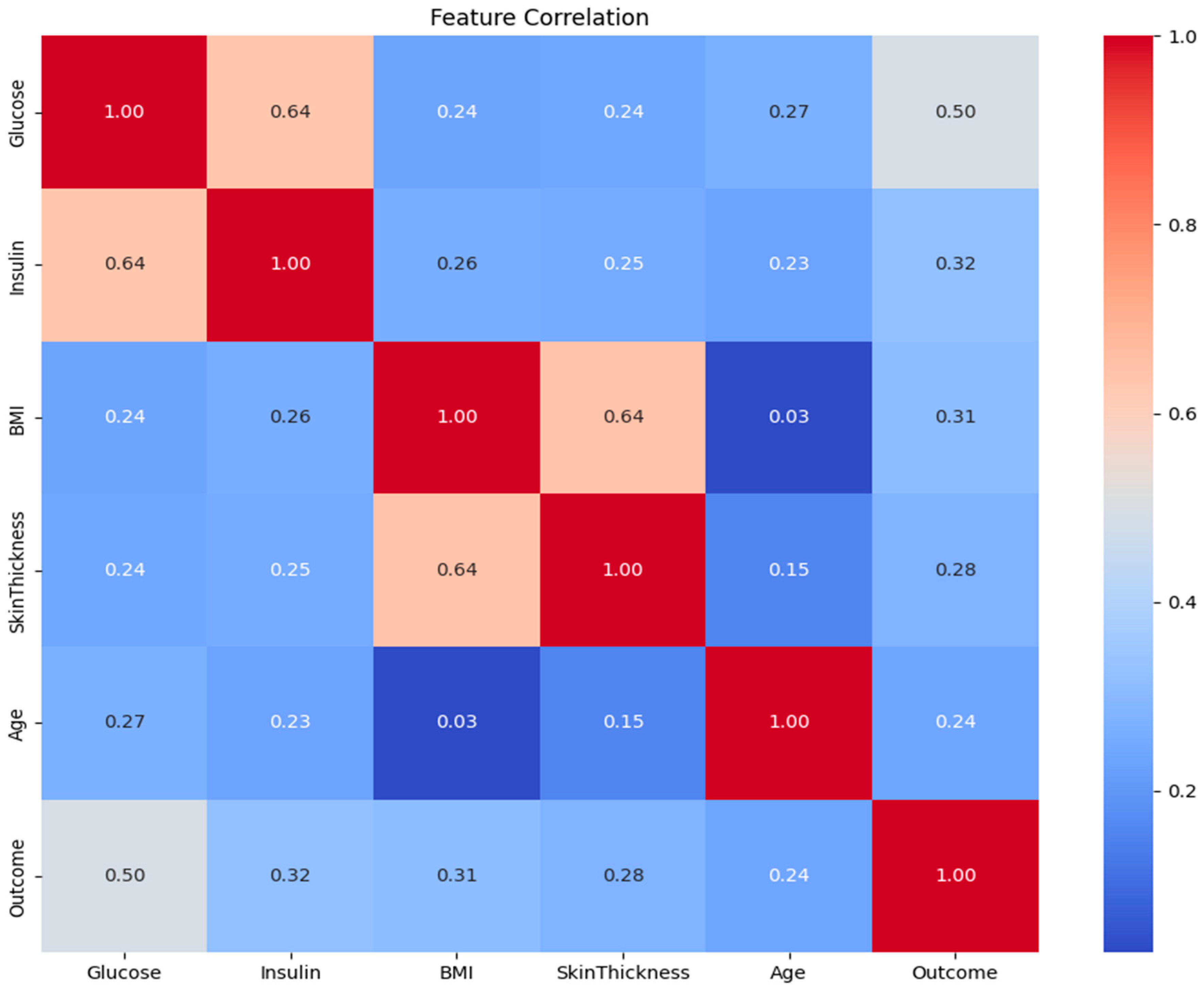
Figure 2. Pearson correlation matrix of the dataset features.
Futureinternet 17 00513 g002
Figure 3. ROC curves for the Random Forest model across all 5 cross-validation folds.
Futureinternet 17 00513 g003
Figure 4. Feature Importance and SHAP analysis.
Futureinternet 17 00513 g004
Figure 5. Mean SHAP value.
Futureinternet 17 00513 g005
Figure 6. Box Plot of Age by Outcome. Green represents non-diabetic patients (Outcome = 0) and orange represents diabetic patients (Outcome = 1). Circles indicate individual outlier values outside the normal range.
Futureinternet 17 00513 g006
Figure 7. Box Plot of Glucose by Outcome. Green represents non-diabetic patients (Outcome = 0) and orange represents diabetic patients (Outcome = 1). Circles indicate outlier data points with glucose levels beyond the normal range.
Futureinternet 17 00513 g007
Table 2. Processed Dataset Statistics (After KNN Imputation).
FeatureCountMeanStd DevMin25%50%75%Max
Glucose768121.730.056.099.0117.0141.0199.0
BloodPressure76871.312.438.064.072.080.0122.0
SkinThickness76829.110.17.022.029.035.099.0
Insulin768155.1100.215.087.0130.5200.0744.0
BMI76832.56.818.228.032.036.667.1
Table 3. Dataset Statistics Before and After Class Balancing with SMOTEENN.
FeatureStageCountMeanStd DevMin25%50%75%Max
GlucoseBefore614121.6730.0356.0099.00117.00140.00199.00
GlucoseAfter448126.6134.0656.00100.00120.00156.26199.00
InsulinBefore614149.3689.7515.0087.00135.00187.25744.00
InsulinAfter448156.0099.4215.0083.18138.71193.14543.00
BMIBefore61432.436.8318.2027.6232.4036.5067.10
BMIAfter44833.237.7918.2027.7832.8037.5067.10
SkinThicknessBefore61429.059.347.0023.0029.0034.5499.00
SkinThicknessAfter44829.099.117.0022.1129.8635.0056.00
AgeBefore61433.3711.8321.0024.0029.0041.0081.00
AgeAfter44832.3210.5021.0024.0029.0040.0072.00
Table 4. Hyperparameter configurations for the evaluated machine learning models.
ModelTuned HyperparametersFull Search SpaceFinal Values
XGBoostn_estimators, max_depth, learning_rate, subsamplen_estimators: [100, 200, 500]; max_depth: [3, 6, 9]; learning_rate: [0.01, 0.1, 0.2]; subsample: [0.8, 1.0]200, 6, 0.1, 0.8
CatBoostiterations, depth, l2_leaf_regiterations: [500, 1000]; depth: [4, 6, 8]; l2_leaf_reg: [1, 3, 5]1000, 6, 3
LightGBMn_estimators, num_leaves, learning_raten_estimators: [100, 200, 500]; num_leaves: [15, 31, 63]; learning_rate: [0.01, 0.1, 0.2]200, 31, 0.1
Random Forest (RF)n_estimators, max_depth, min_samples_leafn_estimators: [100, 200, 500]; max_depth: [10, 20, None]; min_samples_leaf: [1, 2, 4]200, 20, 2
SVMC, gammaC: [0.1, 1, 10, 100]; gamma: [‘scale’, ‘auto’, 0.1, 0.01]10, ‘scale’
KNNn_neighborsn_neighbors: [3, 5, 7, 9, 11]7
Logistic Regression (LR)C, penaltyC: [0.1, 1, 10, 100]; penalty: [‘l2’]1, ‘l2’
AdaBoostn_estimators,
learning_rate
n_estimators: [50, 100, 200]; learning_rate: [0.01, 0.1, 1.0]200, 0.1
Gradient Boosting (GB)n_estimators, learning_rate, max_depthn_estimators: [100, 200, 500]; learning_rate: [0.01, 0.1, 0.2]; max_depth: [3, 4, 5]200, 0.1, 3
Table 7. Comparative performance analysis of the proposed methodology compared to the existing state-of-the-art in diabetes prediction.
ModelDatasetROC-AUCAccuracyF1-ScorePrecisionRecall
LR (Baseline) Pima0.8510.7790.6750.8720.983
CatBoost (Proposed) Pima0.9720.9680.9710.9560.987
LSTM [41] Pima0.8900.8500.8000.8200.780
SVM with PCA [42] Pima0.9290.8610.8870.8890.869
LR [43] Pima0.8250.7680.7600.7630.768
ANN [24] Kaggle0.6800.5900.6600.560
CNN [24]Kaggle0.7700.6000.6900.550
LSTM [24]Kaggle0.7800.6100.7300.530
Table 8. Performance of the CatBoost model on different K imputations.
Metrick = 4k = 6k = 7k = 8
Precision 0.9500.9520.9560.952
Accuracy 0.9650.9530.9680.962
Recall 0.9870.9630.9870.979
F1-Score 0.9680.9580.9710.965
ROC AUC 0.9710.9690.9720.969
PR AUC 0.9720.9710.9720.969
Table 10. Model Performance Summary with 0.95 CI.
ModelROC AUCF1-ScoreAccuracyPrecisionRecall
CatBoost 0.972 [0.965, 0.977]0.971 [0.955, 0.984]0.968 [0.953, 0.984]0.9560.987
RF 0.971 [0.965, 0.976]0.959 [0.937, 0.976]0.955 [0.938, 0.973]0.9630.955
KNN 0.971 [0.964, 0.977]0.951 [0.929, 0.969]0.949 [0.926, 0.969]0.9820.922
XGBoost 0.966 [0.957, 0.974]0.957 [0.939, 0.973]0.953 [0.933, 0.971]0.9630.951
LightGBM 0.966 [0.956, 0.975]0.959 [0.940, 0.975]0.955 [0.935, 0.975]0.9590.959
SVM 0.963 [0.950, 0.973]0.958 [0.938, 0.975]0.953 [0.931, 0.973]0.9440.971
AdaBoost 0.963 [0.953, 0.970]0.943 [0.920, 0.964]0.937 [0.915, 0.960]0.9420.942
GB 0.961 [0.949, 0.971]0.944 [0.922, 0.964]0.940 [0.917, 0.960]0.9460.942
LR 0.951 [0.939, 0.962]0.925 [0.900, 0.948]0.913 [0.884, 0.938]0.8720.984
Table 11. Model Performance on CDC BRFSS 2015 Dataset.
ModelAccuracyPrecisionRecallF1ROC AUC
CatBoost 0.9100.9530.8620.9050.967
XGBoost 0.9100.9540.8610.9050.967
LightGBM 0.9070.9390.8710.9040.967
GradientBoost 0.8920.9080.8720.8900.961
AdaBoost 0.8510.8400.8680.8540.936
RandomForest 0.8430.8220.8750.8480.923
KNN 0.8090.7450.9390.8310.897
SVM 0.8110.7930.8420.8170.887
LogisticRegression 0.7570.7430.7850.7630.832
Table 12. Model Performance on Diabetes 130-US Hospitals Dataset.
ModelAccuracyPrecisionRecallF1ROC AUC
LightGBM 0.9330.9940.8710.9280.959
XGBoost 0.9320.9870.8750.9280.957
CatBoost 0.9310.9890.8680.9260.955
RandomForest 0.8650.8860.8390.8620.933
LogisticRegression 0.6060.6100.5880.5990.650
Table 13. Performance Comparison of Top Ensemble Models Across All Datasets.
DatasetModelAccuracyPrecisionRecallF1-ScoreROC AUC
Pima Indian CatBoost0.9680.9560.9870.9710.972
Pima Indian XGBoost0.9530.9620.9500.9560.966
Pima Indian LightGBM0.9550.9580.9580.9580.966
CDC BRFSS 2015 CatBoost0.9100.9530.8620.9050.967
CDC BRFSS 2015 XGBoost0.9100.9530.8610.9050.967
CDC BRFSS 2015 LightGBM0.9070.9390.8710.9040.967
Diabetes 130-US Hospitals CatBoost0.9310.9890.8680.9260.955
Diabetes 130-US Hospitals XGBoost0.9320.9870.8750.9280.957
Diabetes 130-US Hospitals LightGBM0.9330.9890.8710.9280.959
Disclaimer/Publisher’s Note: The statements, opinions and data contained in all publications are solely those of the individual author(s) and contributor(s) and not of MDPI and/or the editor(s). MDPI and/or the editor(s) disclaim responsibility for any injury to people or property resulting from any ideas, methods, instructions or products referred to in the content.