Beyond Accuracy: Benchmarking Machine Learning Models for Efficient and Sustainable SaaS Decision Support

Abstract

Machine learning (ML) methods have been successfully employed to support decision-making for Software as a Service (SaaS) providers. While most of the published research primarily emphasizes prediction accuracy, other important aspects, such as cloud deployment efficiency and environmental impact, have received comparatively less attention. It is also critical to effectively use factors such as training time, prediction time and carbon footprint in production. SaaS decision support systems use the output of ML models to provide actionable recommendations, such as running reactivation campaigns for users who are likely to churn. To this end, in this paper, we present a benchmarking comparison of 17 different ML models for churn prediction in SaaS, which include cloud deployment efficiency metrics (e.g., latency, prediction time, etc.) and sustainability metrics (e.g., CO₂ emissions, consumed energy, etc.) along with predictive performance metrics (e.g., AUC, Log Loss, etc.). Two public datasets are employed, experiments are repeated on four different machines, locally and on the cloud, while a new weighted Green Efficiency Weighted Score (GEWS) is introduced, as steps towards choosing the simpler, greener and more efficient ML model. Experimental results indicated XGBoost and LightGBM as the models capable of offering a good balance on predictive performance, fast training, inference times, and limited emissions, while the importance of region selection towards minimizing the carbon footprint of the ML models was confirmed.

1. Introduction

SaaS refers to cloud-based application services without the need for installation or local maintenance [1]. The applications are, therefore, hosted by providers, can be accessed from any device as long as there is an internet connection, and are typically under a recurring subscription. SaaS has empowered businesses and individuals with flexibility, lower costs and fast deployment [2]. Yet, billing issues, low engagement, lack of product fit to customer needs and vivid competition between different SaaS tools may lead to churn [3,4]. Customers cancel or fail to renew their subscription, which directly impacts providers’ revenue, growth and long-term viability.

In a SaaS environment, machine learning (ML) models are often employed towards real-time decision support. In this context, ML models repeatedly analyze users’ engagement metrics and behavior, along with transactional data, to determine potential churn risks and provide actionable recommendations such as running reactivation campaigns for users that are likely to churn [3,5]. For the latter task, speed and cost-efficiency are considered crucial for sustainable SaaS ML models; real-time inference is essential to timely provide information for signs of disengagement, while efficient models are required to reduce overheads, considering the related costs to run ML models at scale in cloud resources. Thus, it is important to ensure that ML models are able to provide accurate, fast and cost-efficient predictions to assure sustainability in cloud environments [6]. The environmental footprint of cloud-based ML in SaaS is also a great concern, since nowadays, sustainability is a competitive edge, influencing decisions of customers that increasingly tend to favor SaaS providers with green AI practices [1,7]. Sustainable AI refers to the development and use of AI systems in ways that minimize their environmental impact, promoting long-term ecological and social well-being [8]. Sustainability in cloud environments focuses on the optimal cloud infrastructure so as to reduce energy consumption and carbon emissions [9]. Moreover, it should be noted that, especially in Europe, regulations regarding carbon accountability, such as the EU AI Act [10], are becoming obligatory.

To this end, this work examines ML in SaaS for churn prediction. The aim is to benchmark several ML models, regarding speed, efficiency and emissions. In this work, a total of 17 ML models are tested, and two public datasets are employed for transparency and reproducibility. Results on energy consumption, emissions, training time and prediction time (latency, Throughput), are provided, as well as predictive performance measures AUC (classic) and Log loss, which are valuable for SaaS providers. Moreover, experiments in different cloud settings are performed to show how it affects the generated emissions. In this context, we introduce a Green Efficiency Weighted Score (GEWS) to evaluate ML models based on all these aspects towards choosing simpler and greener alternatives while not sacrificing predicting performance. More specifically, the contributions of this work can be summarized in the following points:

• The benchmarking of 17 ML models in SaaS for churn prediction. Related works also focus on benchmarking ML models in SaaS for churn prediction, yet, the proposed work is the first to examine such an extended set of ML models; Sanches et al. [4] examined seven ML models, Rahman et al. [11] examined four models, Tékouabou et al. [12] examined six models, De Lima Lemos et al. [13] examined six models, Al-Najjar et al. [14] examined five models, Suh [15] examined one model, Lalwani et al. [16] examined four models, Rautio [17] used three models and Maan et al. [18] used four models. Moreover, a literature review on ML in SaaS [6] highlights that the recent literature on ML methods used for decision support in SaaS, including churn prediction, has not reported a single work benchmarking more than 12 ML models.
• An exhaustive evaluation using predictive, efficiency and sustainability measures for SaaS churn prediction, which, to the best of our knowledge, is first reported in the literature covering all those aspects in such an exhaustive experimental setup.
• Employment of two public datasets, KKBOX and Telco. Related works mainly use private datasets; while working with public sets, no benchmark results have been presented together for both datasets, KKBOX and Telco. KKBOX has been used separately [19,20,21,22]; the same applies to the Telco dataset [23,24,25,26].
• Presentation of multiple experiments (PC, Google Cloud VMs, different Regions), focusing on cloud-based environments in realistic circumstances for SaaS applications. Specifically, experiments are performed in three different regions (the United States (US), Europe and Asia) in Google Cloud VMs, with both datasets. The differences when using VMs in different regions and times have already been investigated by Dodge et al. in [27]. The authors explicitly measured operational emissions across different cloud regions and times of day (on Microsoft Azure) and concluded that region choice had the largest impact. It should be noted that most of the related research focused solely on the accuracy of the predictions, neglecting aspects such as cloud deployment efficiency and environmental impact.
• Calculation of carbon emissions and energy consumption. Together with Dodge et al. [27], there is only one work, that of Sanchez Ramirez et al. [28], that assessed the carbon footprint of machine learning models for SaaS decision support. The authors examined the use of usage data for churn prediction and assessed the carbon footprint of five different machine learning models. Yet, the calculation of carbon footprint was conducted based on the estimation of energy consumption rather than real-time computation.
• Benchmark against training time, prediction time (latency) and Throughput in cloud-based systems that are important for production-ready systems.
• Benchmark relative gain in predictive performance over energy consumption and emissions again to identify the most eco-friendly ML models to use for churn prediction in SaaS (AUC/Emissions, Log Loss/Emissions).
• Exhausting investigation of trade-offs between performance–efficiency based on the Pareto frontier analysis.
• Introduction of a novel metric, namely the GEWS, defined as a weighted sum of normalized metrics AUC, Log Loss, training time, Total Emissions and Mean Latency, aiming to evaluate ML models based on all these aspects towards choosing simpler, greener and efficient ML models.

While the proposed methodology uses well-known ML models, its scientific novelty mainly lies in its multi-dimensional and sustainable-aware benchmarking framework, focused on ML-based churn prediction in SaaS environments. The proposed methodology includes an unprecedented range of models’ benchmarking, a holistic evaluation framework, a realistic cloud-based experimental deployment and a novel metric to guide the selection of greener and more efficient ML models. Based on the above, this work aims to provide a framework that combines AI performance, cloud engineering and environmental sustainability, a combination not previously fully explored in the academic literature.

The rest of the paper is structured as follows. Section 2 presents materials and methods used in this work. Results for all experiments are included in Section 3. Section 4 discusses the results, while Section 5 concludes the paper.

2. Materials and Methods

2.1. Proposed Methodology

The proposed methodology is illustrated in Figure 1. First, the data used for the experiments were acquired. Two public datasets were used for our experimentation process to make our work more transparent and reproducible, as most of the related work uses private datasets, making it harder to evaluate the relative performance of different ML methods on SaaS decision support. In the next step, preprocessing of the datasets took place and they were split into a train and holdout set. The preprocessing involved the steps of handling missing values, encoding categorical variables and feature scaling (after splitting the datasets into folds and train/holdout). The data were split into two parts, 80% and 20%, using stratification based on the class variable that represents whether a user would churn or not. The percentage of 80% was used for performing 10-fold cross-validation (CV), while the 20% was used as a holdout set. For handling a class imbalance of the target variable, sample weighting was used, which computes a per-instance weight by giving the minority class larger weights.

A total of 17 different ML algorithms were tested on the same folds and train/holdout set. The selection of models was based on their reported performance for churn prediction as indicated in [6], while classic ML methods were also considered. For each of the ML methods tracked we calculated performance, efficiency and sustainability metrics. All experiments were conducted on four different machines, on a PC and on three Google Cloud Virtual Machines (VMs), each in a different geographical region.

2.2. Datasets

The Telco Customer Churn dataset [29], available at https://www.kaggle.com/datasets/blastchar/telco-customer-churn (accessed on 12 September 2025), is a public dataset widely used in churn prediction research [30]. It contains data from a telecommunication company operating on a subscription basis. Although it is not exactly SaaS, its subscription nature offers quite a similar structure, and thus it has been used in research for SaaS churn prediction [30,31]. In particular, Telco operates on a subscription basis similar to SaaS. The profitability of subscription-based companies generally depends on customer retention. So even small changes in churn rate can significantly impact the generated revenue. Telco contains features such as tenure, contract type, payment method and service usage, which resemble SaaS feature variables such as subscription length, plan type, payment method and product usage. Specifically, it consists of 7043 rows, each one representing one customer, and 21 columns (features) containing information regarding customer attributes, services’ content and subscription.

The second public dataset employed in this study is the one provided by KKBOX’s Churn prediction challenge [32], available at https://www.kaggle.com/competitions/kkbox-churn-prediction-challenge/ (accessed on 12 September 2025). KKBOX is a music streaming service provider with millions of users. It provides a generous, free subscription plan, by the end of which users either churn or renew. The challenge provided data up to March 2017 and asked the participants to predict churn for April 2017. Since the ground truth for April 2017 is not provided in the dataset, we used data up to February (28 February 2017) and used it to predict churn for March 2017. The provided data are in the form of four different .csv files containing information regarding user characteristics, user logs and subscription information, making it suitable to use for benchmarking churn prediction models. Specifically, the KKBOX dataset contains raw data in four different .csv files:

• train_v2 file, contains the user IDs and whether they have churned (97.0961 records);
• transactions_v2 file, contains information regarding users’ membership, payment plans and payment details (1.048.575 records);
• user_logs_v2 file, contains user logs for daily listening behavior (1.048.575 records);
• members_v3 file, contains user information like city and gender (1.048.575 records).

The dataset was preprocessed so as to obtain data per user, resulting in a dataset of 970.960 records and 35 features, where each row contains information about a specific user. Although KKBOX was released in 2017, it is one of the largest real datasets publicly available [30]; therefore, the age of the dataset does not undermine its relevance and does not limit the practical applicability of our findings.

2.3. Data Preprocessing

The Telco dataset is a relatively clean dataset which contains one row per customer and no missing values. However, it contains many categorical variables. One-hot encoding was used to represent those features with numeric values. The continuous numeric features (TotalCharges and MonthlyCharges) were normalized in the [0,1] using MinMaxScaler, after splitting into train/test to ensure no leakage between them. Finally, the resulting dataset contained 33 features and 7043 rows.

Regarding the KKBOX dataset, the row data from the four .csv files were merged with a left joint in order to maintain all data. Then, we kept only data up to 28 February 2017 for training, while data from March 2017 was kept for testing. Thus, no user logs or transactions for March were contained in the train set. From the transactions file, the most recent transaction represented the current payment state of each user. Based on this information, feature engineering was performed, creating features regarding days since registration, subscription length, month and weekday of registration and last transaction. The user logs file contained log events for the users regarding app usage. So, for a user, there might be more than one row or even none, if the user has no activity. Each row contained the user ID, date and features regarding listening activity:

• num_25/50/75/985/100, refers to the number of songs played less than 25%, 25–50%, 50–75%, 75–98.5% and 98.5–100% of the song length;
• num_unq refers to unique songs played;
• total_secs refers to the total seconds played.

We grouped those rows per user and computed sums and means for num_25/50/75/985/100, num_unq and total_secs. From the date column, date_min, date_max and date_unique were derived from the user’s earliest log date, latest log date and number of active days. Then, the following features were defined:

• log_span_days, as date_max minus date_min, to represent user lifespan;
• avg_secs_per_song, defined as the sum of total_secs for each user divided by the number of unique songs played (sum of num_unq);
• days_since_last_log_missing, which is 1 if there are no logs, otherwise it is 0;
• days_since_last_log, for the number of days since the last log.

Following feature engineering, the handling of missing values took place. For the transactional related features like payment_plan_days and actual_amount_paid, we filled missing values with zero. Similarly, user log features were filled with zero when there were no values to show the absence of user activity and the days_since_last_log feature was filled with 999 since zero would mean very recent activity. Columns of raw dates and IDs (msno, bd, registration_init_time, membership_expire_date and transaction_date) were removed. Next, the categorical variable gender was encoded to integer values 1 and 2. For continuous numeric features like “payment_plan_days” and “actual_amount_paid”, normalization was performed by applying MinMaxScaler, separately for the train and test sets. The resulting dataset contained 970.960 rows and 35 features.

2.4. Machine Learning Models

Stratified splits of 80–20% were performed for both datasets to formulate the train and holdout sets. The percentage of 80% was used for performing a 10-fold stratified cross-validation. The splits were saved, and all ML classifiers were trained and tested in the same parts. The utility function of sklearn compute_sample_weight with class_weight = ‘balanced’ was used as a universal way to handle class imbalance [33]. This function computes sample weights, assigning larger values to the minority class, which is used when training the ML model.

The ML methods used in our benchmarking study were selected based on the related research on SaaS decision support in [6], specifically for churn prediction. Therefore, according to the literature review conducted in [6], the most reported ML models for churn prediction in SaaS were selected. In our benchmark, we included Random Forest, which was proposed for SaaS Churn prediction in [31,34,35,36], XGBoost, which was efficiently used in [37,38], Decision Tree used in [5], LightGBM proposed in [39] and Logistic Regression reported in [28]. Moreover, we used a multi-layer perceptron (MLP) for including feed-forward neural network (NN) implementation in our experiments, as in [40,41]. Similarly, we used a Stacking ensemble (StackGBM), as proposed in the recent publication of Li [42], which uses Random Forest, XGBoost, LightGBM and CatBoost as base learners and XGBoost as a meta-learner. We also included an ensemble combination of XGBoost and LightGBM inspired by the winning solution in the KKBOX Challenge [19]. Two other ensemble combinations were included in order to test their relative performance, VoteAllGBM, which used XGBoost, LightGBM and CatBoost in a soft voting scheme and Vote_Mix, which used XGBoost, Logistic Regression, Decision Tree and Naïve Bayes in a soft voting scheme. Classic ML models such as Multinomial and Bernoulli Naïve Bayes were also included in benchmarking in order to compare their performance with the rest of the selected methods. Finally, the Bagging of Decision Trees, Logistic Regression with stochastic gradient descent (SGD) learning and an ensemble of SGD with Naïve Bayes were also included.

At this point, no deep learning (DL) architectures were selected, despite their relevance in large-scale SaaS. The latter was due to the model selection process that was based on the findings of [6], as well as because DL architectures are not best fitted for tabular data, such as in our case. The use of DL models would require different preprocessing and format of the dataset. Considering DL models in our methodology would be technically possible, yet it would be methodically unfair to compare their results directly with the results obtained by our ML models in the current setup. Moreover, recall the scope of this work, which is to provide a methodology for benchmarking ML models for SaaS churn prediction, focusing on efficiency and sustainability.

Table 1. Parameter setup of ML models used in the benchmarking process.

Model [Ref.]	Setup Parameters
XGBoost [43]	XGBClassifier (eval_metric =“logloss”) (xgboost library)
LightGBM [44]	LGBM classifier (lightgbm library)
CatBoost [45]	CatBoost classifier (catboost library)
Logistic Regression [46]	LogisticRegression (max_iter = 1000)
Decision Tree [47]	DecisionTree
Random Forest [48]	RandomForest
Naïve Bayes [49]	GaussianNB
MLP [50]	MLPClassifier(max_iter = 300)
Vote_XGB_LGBM (Voting of XGBoost and LightGBM)	VotingClassifier. Estimators: XGBClassifier (eval_metric = “logloss”, LGBMClassifier, Voting = “soft”
Vote_AllGBM (Voting of XGBoost, LightGBM and CatBoost)	VotingClassifier. Estimators: XGBClassifier (eval_metric = “logloss”, LGBMClassifier, CatBoostClassifier. Voting = “soft”
Vote_Mix (Voting of XGBoost, Logistic Regression, Decision Tree and Naïve Bayes)	VotingClassifier. Estimators: XGBClassifier (eval_metric = “logloss”), LogisticRegression(max_iter = 1000), DecisionTreeClassifier, GaussianNB. Voting = “soft”
StackGBM (Stacking Ensemble of Random Forest, XGBoost, LightGBM, CatBoost and final estimator XGBoost) [51]	StackingClassifier. Estimators: RandomForestClassifier, XGBClassifier (eval_metric = “logloss”), LGBMClassifier, CatBoostClassifier. Final_estimator: XGBClassifier(use_label_encoder = False, eval_metric = “logloss, passthrough = True))
BernoulliNB [52]	BernoulliNB
Multinomial NB [53]	MultinomialNB
Bagging (Bagging of Decision Trees) [54]	BaggingClassifier. Estimator: DecisionTreeClassifier(n_estimators = 10)
SGD (Logistic Regression with Stochastic Gradient Descent) [55]	SGDClassifier(loss = “log_loss”, max_iter = 2000)
SGD_NB_Ensemble (Voting of SGD and Naïve Bayes)	VotingClassifier. Estimators: SGDClassifier (loss = “log_loss”, max_iter = 2000, GaussianNB()), Voting: soft

contains all the ML models used in our benchmarking. The implementation (in Python 3.11.13) employed Python library scikit-learn 1.7.1 for all ML models except XGBoost, LightGMB and CatBoost, and XGBoost 3.0.3 for XGBoost models, LightGBM 4.6.0 for LightGBM models and CatBoost 1.2.8 for CatBoost models. For all the models, random_state = 42 was set. For all the models, the default hyperparameters were used, as defined in

Table A1. Default parameters of ML models used in the benchmarking process. The rest of the models’ parameters are set to ‘none’.

Model [Ref.]	Default Parameters
XGBoost [43]	‘objective’: ‘binary:logistic’, ‘eval_metric’: ‘logloss’, ‘random_state’: 42, ‘use_label_encoder’: False
LightGBM [44]	‘boosting_type’: ‘gbdt’, ‘colsample_bytree’: 1.0, ‘learning_rate’: 0.1, ‘max_depth’: -1, ‘min_child_samples’: 20, ‘min_child_weight’: 0.001, ‘min_split_gain’: 0.0, ‘num_leaves’: 31, ‘random_state’: 42, ‘reg_alpha’: 0.0, ‘reg_lambda’: 0.0, ‘subsample’: 1.0, ‘subsample_for_bin’: 200,000, ‘subsample_freq’: 0, ‘objective’: ‘binary’, ‘metric’: [‘binary’], ‘num_threads’: 16, ‘num_iterations’: 100
CatBoost [45]	nan_mode: Min, eval_metric: Logloss, iterations: 1000, sampling_frequency: PerTree, leaf_estimation_method: Newton, random_score_type: NormalWithModelSizeDecrease, grow_policy: SymmetricTree, penalties_coefficient: 1, boosting_type: Plain, model_shrink_mode: Constant, feature_border_type: GreedyLogSum, bayesian_matrix_reg: 0.10000000149011612, eval_fraction: 0, force_unit_auto_pair_weights: False, l2_leaf_reg: 3, random_strength: 1, rsm: 1, boost_from_average: False, model_size_reg: 0.5, pool_metainfo_options: {‘tags’: {}}, subsample: 0.800000011920929, use_best_model: False, class_names: [0,1], random_seed: 42, depth: 6, posterior_sampling: False, border_count: 254, classes_count: 0, sparse_features_conflict_fraction: 0, leaf_estimation_backtracking: AnyImprovement, best_model_min_trees: 1, model_shrink_rate: 0, min_data_in_leaf: 1, loss_function: Logloss, learning_rate: 0.020607000216841698, score_function: Cosine, task_type: CPU, leaf_estimation_iterations: 10, bootstrap_type: MVS, max_leaves: 64
Logistic Regression [46]	‘C’: 1.0, ‘dual’: False, ‘fit_intercept’: True, ‘intercept_scaling’: 1, ‘max_iter’: 1000, ‘multi_class’: ‘deprecated’, ‘penalty’: ‘l2’, ‘random_state’: 42, ‘solver’: ‘lbfgs’, ‘tol’: 0.0001, ‘verbose’: 0, ‘warm_start’: False
Decision Tree [47]	‘ccp_alpha’: 0.0, ‘criterion’: ‘gini’, ‘min_impurity_decrease’: 0.0, ‘min_samples_leaf’: 1, ‘min_samples_split’: 2, ‘min_weight_fraction_leaf’: 0.0, ‘random_state’: 42, ‘splitter’: ‘best’
Random Forest [48]	‘bootstrap’: True, ‘ccp_alpha’: 0.0, ‘criterion’: ‘gini’, ‘max_features’: ‘sqrt’, ‘min_impurity_decrease’: 0.0, ‘min_samples_leaf’: 1, ‘min_samples_split’: 2, ‘min_weight_fraction_leaf’: 0.0, ‘n_estimators’: 100, ‘oob_score’: False, ‘random_state’: 42, ‘verbose’: 0, ‘warm_start’: False
Naïve Bayes [49]	‘var_smoothing’: 1e-09
MLP [50]	‘activation’: ‘relu’, ‘alpha’: 0.0001, ‘batch_size’: ‘auto’, ‘beta_1’: 0.9, ‘beta_2’: 0.999, ‘early_stopping’: False, ‘epsilon’: 1e-08, ‘hidden_layer_sizes’: (100,), ‘learning_rate’: ‘constant’, ‘learning_rate_init’: 0.001, ‘max_fun’: 15000, ‘max_iter’: 300, ‘momentum’: 0.9, ‘n_iter_no_change’: 10, ‘nesterovs_momentum’: True, ‘power_t’: 0.5, ‘random_state’: 42, ‘shuffle’: True, ‘solver’: ‘adam’, ‘tol’: 0.0001, ‘validation_fraction’: 0.1, ‘verbose’: False, ‘warm_start’: False
Vote_XGB_LGBM (Voting of XGBoost and LightGBM)	enable_categorical = False, eval_metric = ‘logloss’, missing = nan, (‘lgbm’, LGBMClassifier(random_state = 42))], ‘flatten_transform’: True, ‘verbose’: False, ‘voting’: ‘soft’, ‘xgb’: XGBClassifier(enable_categorical = False, eval_metric = ‘logloss’, missing = nan), ‘lgbm’: LGBMClassifier(random_state = 42), ‘xgb__objective’: ‘binary:logistic’, ‘xgb__enable_categorical’: False, ‘xgb__eval_metric’: ‘logloss’, ‘xgb__missing’: nan, ‘xgb__random_state’: 42, ‘xgb__use_label_encoder’: False, ‘lgbm__boosting_type’: ‘gbdt’, ‘lgbm__colsample_bytree’: 1.0, ‘lgbm__importance_type’: ‘split’, ‘lgbm__learning_rate’: 0.1, ‘lgbm__max_depth’: -1, ‘lgbm__min_child_samples’: 20, ‘lgbm__min_child_weight’: 0.001, ‘lgbm__min_split_gain’: 0.0, ‘lgbm__n_estimators’: 100, ‘lgbm__num_leaves’: 31, ‘lgbm__random_state’: 42, ‘lgbm__reg_alpha’: 0.0, ‘lgbm__reg_lambda’: 0.0, ‘lgbm__subsample’: 1.0, ‘lgbm__subsample_for_bin’: 200,000, ‘lgbm__subsample_freq’: 0
Vote_AllGBM (Voting of XGBoost, LightGBM and CatBoost)	{‘estimators’: [(‘xgb’, XGBClassifier(enable_categorical = False, eval_metric = ‘logloss’, missing = nan)), (‘lgbm’, LGBMClassifier(random_state = 42)), (‘cat’, <catboost.core.CatBoostClassifier object at 0x000002516EF9A0D0 >)], ‘flatten_transform’: True, ‘verbose’: False, ‘voting’: ‘soft’, ‘xgb’: XGBClassifier(enable_categorical = False, eval_metric = ‘logloss’, missing = nan), ‘lgbm’: LGBMClassifier(random_state = 42), ‘cat’: <catboost.core.CatBoostClassifier object at 0x000002516EF9A0D0 >, ‘xgb__objective’: ‘binary: logistic’, ‘xgb__enable_categorical’: False, ‘xgb__eval_metric’: ‘logloss’, ‘xgb__missing’: nan, ‘xgb__random_state’: 42, ‘xgb__use_label_encoder’: False, ‘lgbm__boosting_type’: ‘gbdt’, ‘lgbm__colsample_bytree’: 1.0, ‘lgbm__importance_type’: ‘split’, ‘lgbm__learning_rate’: 0.1, ‘lgbm__max_depth’: -1, ‘lgbm__min_child_samples’: 20, ‘lgbm__min_child_weight’: 0.001, ‘lgbm__min_split_gain’: 0.0, ‘lgbm__n_estimators’: 100, ‘lgbm__num_leaves’: 31, ‘lgbm__random_state’: 42, ‘lgbm__reg_alpha’: 0.0, ‘lgbm__reg_lambda’: 0.0, ‘lgbm__subsample’: 1.0, ‘lgbm__subsample_for_bin’: 200,000, ‘lgbm__subsample_freq’: 0, ‘cat__verbose’: 0, ‘cat__random_state’: 42}
Vote_Mix (Voting of XGBoost, Logistic Regression, Decision Tree and Naïve Bayes)	‘estimators’: [(‘xgb’, XGBClassifier(enable_categorical = False, eval_metric = ‘logloss’, missing = nan)), (‘lr’, LogisticRegression(max_iter = 1000, random_state = 42)), (‘dt’, DecisionTreeClassifier(random_state = 42)), (‘nb’, GaussianNB())], ‘flatten_transform’: True, ‘verbose’: False, ‘voting’: ‘soft’, ‘xgb’: XGBClassifier(enable_categorical = False, eval_metric = ‘logloss’, missing = nan), ‘lr’: LogisticRegression(max_iter = 1000, random_state = 42), ‘dt’: DecisionTreeClassifier(random_state = 42), ‘nb’: GaussianNB(), ‘xgb__objective’: ‘binary:logistic’, ‘xgb__enable_categorical’: False, ‘xgb__eval_metric’: ‘logloss’, ‘xgb__missing’: nan, ‘xgb__random_state’: 42, ‘xgb__use_label_encoder’: False, ‘lr__C’: 1.0, ‘lr__dual’: False, ‘lr__fit_intercept’: True, ‘lr__intercept_scaling’: 1, ‘lr__max_iter’: 1000, ‘lr__multi_class’: ‘deprecated’, ‘lr__penalty’: ‘l2’, ‘lr__random_state’: 42, ‘lr__solver’: ‘lbfgs’, ‘lr__tol’: 0.0001, ‘lr__verbose’: 0, ‘lr__warm_start’: False, ‘dt__ccp_alpha’: 0.0, ‘dt__criterion’: ‘gini’, ‘dt__min_impurity_decrease’: 0.0, ‘dt__min_samples_leaf’: 1, ‘dt__min_samples_split’: 2, ‘dt__min_weight_fraction_leaf’: 0.0, ‘dt__random_state’: 42, ‘dt__splitter’: ‘best’, ‘nb__var_smoothing’: 1e-09
StackGBM (Stacking Ensemble of Random Forest, XGBoost, LightGBM, CatBoost and final estimator XGBoost) [51]	‘estimators’: [(‘rf’, RandomForestClassifier(random_state = 42)), (‘xgb’, XGBClassifier(enable_categorical = False, eval_metric = ‘logloss’, missing = nan, m)), (‘lgbm’, LGBMClassifier(random_state = 42)), (‘cat’, <catboost.core.CatBoostClassifier object at 0x0000025159667F90 >)], ‘final_estimator__objective’: ‘binary:logistic’, ‘final_estimator__enable_categorical’: False, ‘final_estimator__eval_metric’: ‘logloss’, ‘final_estimator__missing’: nan, ‘final_estimator__random_state’: 42, ‘final_estimator__use_label_encoder’: False, ‘final_estimator’: XGBClassifier(enable_categorical = False, eval_metric = ‘logloss’, missing = nan), ‘passthrough’: True, ‘stack_method’: ‘auto’, ‘verbose’: 0, ‘rf’: RandomForestClassifier(random_state = 42), ‘xgb’: XGBClassifier(eval_metric = ‘logloss’, missing = nan), ‘lgbm’: LGBMClassifier(random_state = 42), ‘cat’: <catboost.core. CatBoostClassifier object at 0x0000025159667F90 >, ‘rf__bootstrap’: True, ‘rf__ccp_alpha’: 0.0, ‘rf__criterion’: ‘gini’, ‘rf__max_features’: ‘sqrt’, ‘rf__min_impurity_decrease’: 0.0, ‘rf__min_samples_leaf’: 1, ‘rf__min_samples_split’: 2, ‘rf__min_weight_fraction_leaf’: 0.0, ‘rf__n_estimators’: 100, ‘rf__oob_score’: False, ‘rf__random_state’: 42, ‘rf__verbose’: 0, ‘rf__warm_start’: False, ‘xgb__objective’: ‘binary: logistic’, ‘xgb__enable_categorical’: False, ‘xgb__eval_metric’: ‘logloss’, ‘xgb__missing’: nan, ‘xgb__use_label_encoder’: False, ‘lgbm__boosting_type’: ‘gbdt’, ‘lgbm__colsample_bytree’: 1.0, ‘lgbm__importance_type’: ‘split’, ‘lgbm__learning_rate’: 0.1, ‘lgbm__max_depth’: -1, ‘lgbm__min_child_samples’: 20, ‘lgbm__min_child_weight’: 0.001, ‘lgbm__min_split_gain’: 0.0, ‘lgbm__n_estimators’: 100, ‘lgbm__num_leaves’: 31, ‘lgbm__random_state’: 42, ‘lgbm__reg_alpha’: 0.0, ‘lgbm__reg_lambda’: 0.0, ‘lgbm__subsample’: 1.0, ‘lgbm__subsample_for_bin’: 200,000, ‘lgbm__subsample_freq’: 0, ‘cat__verbose’: 0, ‘cat__random_state’: 42}
BernoulliNB [52]	‘alpha’: 1.0, ‘binarize’: 0.0, ‘fit_prior’: True, ‘force_alpha’: True
MultinomialNB [53]	‘alpha’: 1.0, ‘fit_prior’: True, ‘force_alpha’: True
Bagging (Bagging of Decision Trees) [54]	‘bootstrap’: True, ‘bootstrap_features’: False, ‘estimator__ccp_alpha’: 0.0, ‘estimator__criterion’: ‘gini’, ‘estimator__min_impurity_decrease’: 0.0, ‘estimator__min_samples_leaf’: 1, ‘estimator__min_samples_split’: 2, ‘estimator__min_weight_fraction_leaf’: 0.0, ‘estimator__random_state’: 42, ‘estimator__splitter’: ‘best’, ‘estimator’: DecisionTreeClassifier(random_state = 42), ‘max_features’: 1.0, ‘max_samples’: 1.0, ‘n_estimators’: 10, ‘oob_score’: False, ‘random_state’: 42, ‘verbose’: 0, ‘warm_start’: False
SGD (Logistic Regression with Stochastic Gradient Descent) [55]	‘alpha’: 0.0001, ‘average’: False, ‘early_stopping’: False, ‘epsilon’: 0.1, ‘eta0’: 0.0, ‘fit_intercept’: True, ‘l1_ratio’: 0.15, ‘learning_rate’: ‘optimal’, ‘loss’: ‘log_loss’, ‘max_iter’: 2000, ‘n_iter_no_change’: 5, ‘penalty’: ‘l2’, ‘power_t’: 0.5, ‘random_state’: 42, ‘shuffle’: True, ‘tol’: 0.001, ‘validation_fraction’: 0.1, ‘verbose’: 0, ‘warm_start’: False
SGD_NB_Ensemble (Voting of SGD and Naïve Bayes)	‘estimators’: [(‘SGD’, SGDClassifier(loss = ‘log_loss’, max_iter = 2000, random_state = 42)), (‘nb’, GaussianNB())], ‘flatten_transform’: True, ‘verbose’: False, ‘voting’: ‘soft’, ‘SGD’: SGDClassifier(loss = ‘log_loss’, max_iter = 2000, random_state = 42), ‘nb’: GaussianNB(), ‘SGD__alpha’: 0.0001, ‘SGD__average’: False, ‘’SGD__early_stopping’: False, ‘SGD__epsilon’: 0.1, ‘SGD__eta0’: 0.0, ‘SGD__fit_intercept’: True, ‘SGD__l1_ratio’: 0.15, ‘SGD__learning_rate’: ‘optimal’, ‘SGD__loss’: ‘log_loss’, ‘SGD__max_iter’: 2000, ‘SGD__n_iter_no_change’: 5, ‘SGD__penalty’: ‘l2’, ‘SGD__power_t’: 0.5, ‘SGD__random_state’: 42, ‘SGD__shuffle’: True, ‘SGD__tol’: 0.001, ‘SGD__validation_fraction’: 0.1, ‘SGD__verbose’: 0, ‘SGD__warm_start’: False, ‘nb__var_smoothing’: 1e-09

of the Appendix A Section.

Table A2. Implementation links for all models.

Model [Ref.]	Implementation Links
XGBoost [43]	https://xgboost.readthedocs.io/en/stable/parameter.html (assessed on 12 September 2025)
LightGBM [44]	https://lightgbm.readthedocs.io/en/latest/Parameters.html (assessed on 12 September 2025)
CatBoost [45]	https://catboost.ai/docs/en/references/training-parameters/ (assessed on 12 September 2025)
Logistic Regression [46]	https://scikit-learn.org/stable/modules/generated/sklearn.linear_model.LogisticRegression.html#sklearn.linear_model.LogisticRegression (assessed on 12 September 2025)
Decision Tree [47]	https://scikit-learn.org/stable/modules/generated/sklearn.tree.DecisionTreeClassifier.html#sklearn.tree.DecisionTreeClassifier (assessed on 12 September 2025)
Random Forest [48]	https://scikit-learn.org/stable/modules/generated/sklearn.ensemble.RandomForestClassifier.html#sklearn.ensemble.RandomForestClassifier (assessed on 12 September 2025)
Naïve Bayes [49]	https://scikit-learn.org/stable/modules/generated/sklearn.naive_bayes.GaussianNB.html#sklearn.naive_bayes.GaussianNB (assessed on 12 September 2025)
MLP [50]	https://scikit-learn.org/stable/modules/generated/sklearn.neural_network.MLPClassifier.html#sklearn.neural_network.MLPClassifier (assessed on 12 September 2025)
Vote_XGB_LGBM (Voting of XGBoost and LightGBM)	https://scikit-learn.org/stable/modules/generated/sklearn.ensemble.VotingClassifier.html#sklearn.ensemble.VotingClassifier (assessed on 12 September 2025)
Vote_AllGBM (Voting of XGBoost, LightGBM and CatBoost)	https://scikit-learn.org/stable/modules/generated/sklearn.ensemble.VotingClassifier.html#sklearn.ensemble.VotingClassifier (assessed on 12 September 2025)
Vote_Mix (Voting of XGBoost, Logistic Regression, Decision Tree and Naïve Bayes)	https://scikit-learn.org/stable/modules/generated/sklearn.ensemble.VotingClassifier.html#sklearn.ensemble.VotingClassifier (assessed on 12 September 2025)
StackGBM (Stacking Ensemble of Random Forest, XGBoost, LightGBM, CatBoost and final estimator XGBoost) [51]	https://scikit-learn.org/stable/modules/generated/sklearn.ensemble.StackingClassifier.html#sklearn.ensemble.StackingClassifier (assessed on 12 September 2025)
BernoulliNB [52]	https://scikit-learn.org/stable/modules/generated/sklearn.naive_bayes.BernoulliNB.html (assessed on 12 September 2025)
MultinomialNB [53]	https://scikit-learn.org/stable/modules/generated/sklearn.naive_bayes.MultinomialNB.html (assessed on 12 September 2025)
Bagging (Bagging of Decision Trees) [54]	https://scikit-learn.org/stable/modules/generated/sklearn.ensemble.BaggingClassifier.html#sklearn.ensemble.BaggingClassifier (assessed on 12 September 2025)
SGD (Logistic Regression with Stochastic Gradient Descent) [55]	https://scikit-learn.org/stable/modules/generated/sklearn.linear_model.SGDClassifier.html#sklearn.linear_model.SGDClassifier (assessed on 12 September 2025)
SGD_NB_Ensemble (Voting of SGD and Naïve Bayes)	https://scikit-learn.org/stable/modules/generated/sklearn.ensemble.VotingClassifier.html#sklearn.ensemble.VotingClassifier (assessed on 12 September 2025)

of the Appendix A Section also provides the referenced implementation links for all models, aiming to provide full access to the readers to source codes towards reproducing the benchmarking process. In case a specific value of a hyperparameter, different from the default is used, it is mentioned in Table 1.

In this work, optimization of the models’ hyperparameters is not considered. Hyperparameter tuning can enhance model performance and potentially affect comparative fairness. However, our decision to evaluate all models using default hyperparameters was intentional, due to the following reasons: (1) to establish a reproducible benchmarking baseline across all models, allowing for a fair comparison of models in their most accessible form; (2) to align with our sustainability goals and reflect realistic deployment scenarios where tuning may not be feasible due to resource constrains; (3) to train and evaluate all models under the same conditions, pursuing fairness through uniformity, ensuring methodological consistency and avoiding bias introduced by uneven tuning efforts.

2.5. Training and Evaluation

The experimentation process was conducted in four different machines by following the same steps. First, the preprocessing of the datasets was made as explained in Section 2.2, as well as the splitting into train/test (folds) and holdout sets. Then, all the ML models were trained in the same folds, performing 10-fold CV. Finally, the ML models were trained in the full training set and tested with the holdout set.

The process was repeated in four different machines, a PC and three Google Cloud VMs in different regions. The deployment of the SaaS prediction models could be performed in various ways, for example, using serverless containers such as Cloud Run or platforms like VertexAI. However, those environments offer less control compared to VMs, making them unsuitable for reliably tracking energy consumption and emissions. Therefore, for the proposed benchmarking study, VMs were used for reliably measuring energy consumption and emissions.

More specifically, first, all experiments were conducted on a PC Intel i5-9400F, 64-bit RAM, 32 GB with Ubuntu 24.04.3 LTS, 64-bit kernel, which runs in Kavala, Greece. In Google Cloud, we set 3 VMs of type c4-standard-4 [56] (4 vCPUs, 15 GB Memory) in regions in Asia (Tokyo), Europe (Frankfurt) and the USA (Oregon). The generated emissions differ among different regions due to the way energy is produced.

Table 2. Google Cloud VMs, regions and grid carbon intensity.

VM	Google Cloud Region	Location	Grid Carbon Intensity (gCO2eq/kWh)	CO2 Intensity Characterization
VM1	asia-northeast1-b 19:00 UTC	Asia (Tokyo)	453	High
VM2	europe-west3 19:00 UTC	Europe (Frankfurt)	276	Medium
VM3	us-west1 19:00 UTC	US (Oregon)	>200	High

includes the selected regions and grid carbon intensity (gCO₂eq/kWh) as reported in the “Carbon free energy for Google Cloud regions” report, available at https://cloud.google.com/sustainability/region-carbon (accessed on 12 September 2025). As it is shown in Table 2, VM3 is the “greenest” option since it is considered “Low CO₂”, VM2 is of medium grid carbon intensity and VM1 is of high grid carbon intensity. This setup aims to measure the relative differences in the emissions generated by running the same ML models in regions with different grid carbon intensities.

For all experiments, the evaluation metrics included in

Table 3. Evaluation metrics per objective.

Evaluation Metrics	Objective
AUC	Predictive performance
Log-Loss
Accuracy
Precision
Recall
F-measure
Training time	Efficiency
Prediction time
Mean Latency
Throughput
Model Size	Sustainability
Energy_consumed
Emissions CO2

are calculated. Predictive performance metrics include classic metrics like AUC, accuracy, precision, recall and F-measure, as well as Log Loss, which is the evaluation metric used in KKBOX challenges, and it is considered valuable for SaaS providers running reactivation campaigns. For the calculation of energy consumption and emissions generated, the CodeCarbon library available at https://codecarbon.io/ (accessed on 12 September 2025) was used. CodeCarbon monitors energy consumption when running code and maps it to carbon emissions based on the carbon intensity of electricity in the region where the code is running. Energy consumption and CO₂ emissions, along with model size and training time, were tracked for both 10-fold CV and train/holdout experiments. Prediction time, Mean Latency and Throughput were calculated by loading the saved ML models that were trained in the full train set, predicting the output for the complete holdout set.

3. Results

In this section, the experiment results are presented. Section 3.1 presents the results regarding the predictive performance of the ML models, efficiency is evaluated in Section 3.2 and sustainability in Section 3.3., either on PC or on the cloud. Trade-offs between performance and efficiency are discussed in Section 3.4, concluding with the introduction of a novel Green Efficiency Weighted Score (GEWS) aiming to help identify both the most efficient and greener alternatives.

3.1. Performance Evaluation

Apart from accuracy, precision, recall and F1-score, a common evaluation metric for churn prediction is the Area Under the Curve (AUC). AUC shows how well the model can separate churners from non-churners. Additionally, Log Loss is also calculated, as it is the evaluation metric used in the KKBOX challenge. Log Loss is considered important for SaaS providers because it is linked to the reliability of predictions of churn models for each user. SaaS vendors use them to select which users to target in their retention campaigns. Retention campaigns can become costly, so it is essential to target the right users to ensure resources are used efficiently and not wasted.

The Log Loss value for an instance with true class label $y\in$ {0,1} and probability estimate p for y = 1 is defined as shown in Equation (1) [57]:

$$L{og Loss}_i\left(y,p\right)=-(y\ast (\log \left(p\right)+\left(1-y\right)\ast \mathrm{l}\mathrm{o}\mathrm{g}(1-p)$$

(1)

Then, for N instances, the average Log Loss value is computed.

3.1.1. Performance on 10-Fold CV

Table 4. Evaluation metrics for 10-fold CV on dataset KKBOX (PC).

ML Model	Mean Accuracy	Mean Precision	Mean Recall	Mean F1-Score	Mean AUC (CV)	Mean Log Loss (CV)
XGBoost	0.72	0.21	0.74	0.32	0.80	0.52
LightGBM	0.72	0.21	0.74	0.32	0.80	0.52
CatBoost	0.73	0.21	0.73	0.32	0.80	0.52
Logistic Regression	0.71	0.16	0.53	0.25	0.68	0.63
Decision Tree	0.83	0.24	0.42	0.30	0.59	2.51
Random Forest	0.85	0.27	0.37	0.31	0.64	0.73
Naïve Bayes	0.85	0.18	0.19	0.18	0.67	2.04
MLP	0.73	0.21	0.71	0.32	0.79	0.54
Vote_XGB_LGBM	0.92	0.93	0.16	0.27	0.80	0.24
Vote_AllGBM	0.92	0.92	0.16	0.27	0.80	0.24
Vote_Mix	0.92	0.75	0.16	0.26	0.74	0.27
StackGBM	0.92	0.91	0.16	0.27	0.80	0.24
BernoulliNB	0.75	0.15	0.37	0.21	0.64	0.81
MultinomialNB	0.82	0.17	0.26	0.20	0.66	0.66
Bagging	0.86	0.27	0.36	0.31	0.64	1.16
SGD	0.71	0.16	0.54	0.25	0.68	0.64
SGD_NB_Ensemble	0.85	0.18	0.19	0.18	0.66	0.33

presents the evaluation results for the 10-fold CV in the KKBOX dataset. As it is shown, XGBoost, CatBoost, LightGBM and the ensemble approaches Voting and Stacking (Vote_AllGBM, Vote_XGB_LGBM and StackGBM) achieved an AUC of 0.80. Similarly, MLP achieved an AUC of 0.79. The rest of the ML models noted an AUC value of less than 0.75. Specifically, Vote_Mix noted an AUC of 0.74, Logistic Regression of 0.68, Naïve Bayes of 0.67, MultinomialNB of 0.66 and BernoulliNB of 0.64. Bagging noted an AUC of 0.64, while SGD and SGD_NB_Ensemble, of 0.68 and 0.66, respectively.

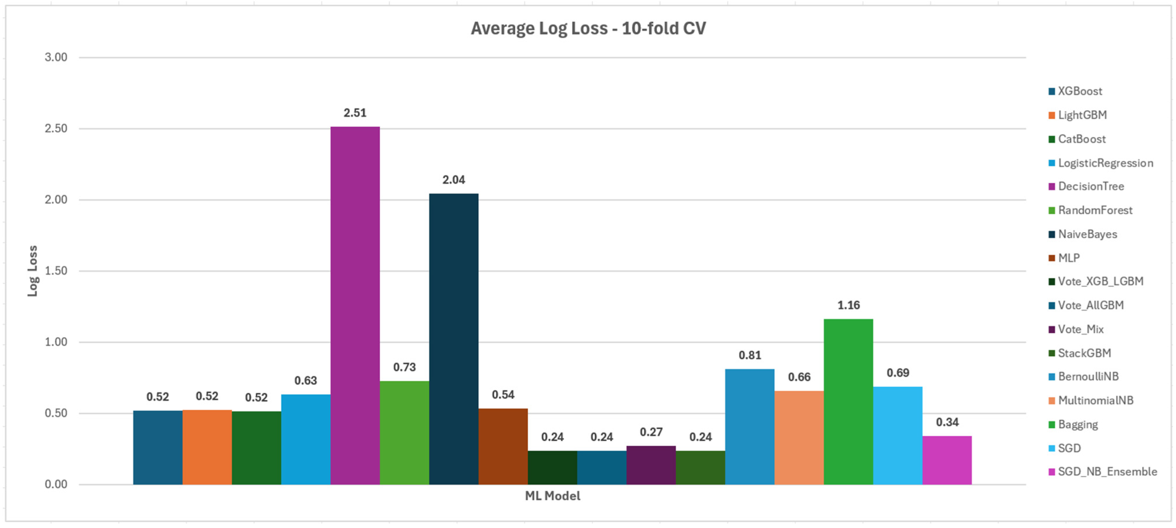
Regarding Log Loss values, the best results were noted by the ensemble approaches Vote_AllGBM, Vote_XGB_LGBM and StackGBM, which showed Log Loss values of 0.24 and Vote_Mix of 0.27. The ML models SGD_NB_Ensemble showed a relatively good Log Loss of 0.33, while CatBoost and XGBoost followed with 0.52. MLP noted a similar Log Loss of 0.54, while the rest of the ML models followed with mediocre results ranging from 0.63 for Logistic Regression to 2.51 for Decision Tree.

Figure 2 illustrates the AUC for each of the ML models, while Figure 3 illustrates the Log Loss. Although ensemble approaches Vote_AllGBM, Vote_XGB_LGBM and StackGBM reported the best results in Log Loss, they showed low levels of recall (less than 0.2) and high precision (0.75–0.92). Thus, those ML models could be characterized as “conservative” in terms of predicting churned users. However, when they characterize a user as churned, their decision is mostly accurate.

XGBoost, CatBoost and LightGBM achieved the best results in recall (0.74, 0.74 and 0.73, respectively), indicating that they can classify most churners correctly. MLP showed similar results with 0.71 recall. Therefore, for SaaS providers that run expensive campaigns and want to minimize the risk of targeting users that are not likely to churn, ML models such as Vote_AllGBM, Vote_XGB_LGBM and StackGBM are a better fit (based only on the predictive performance).

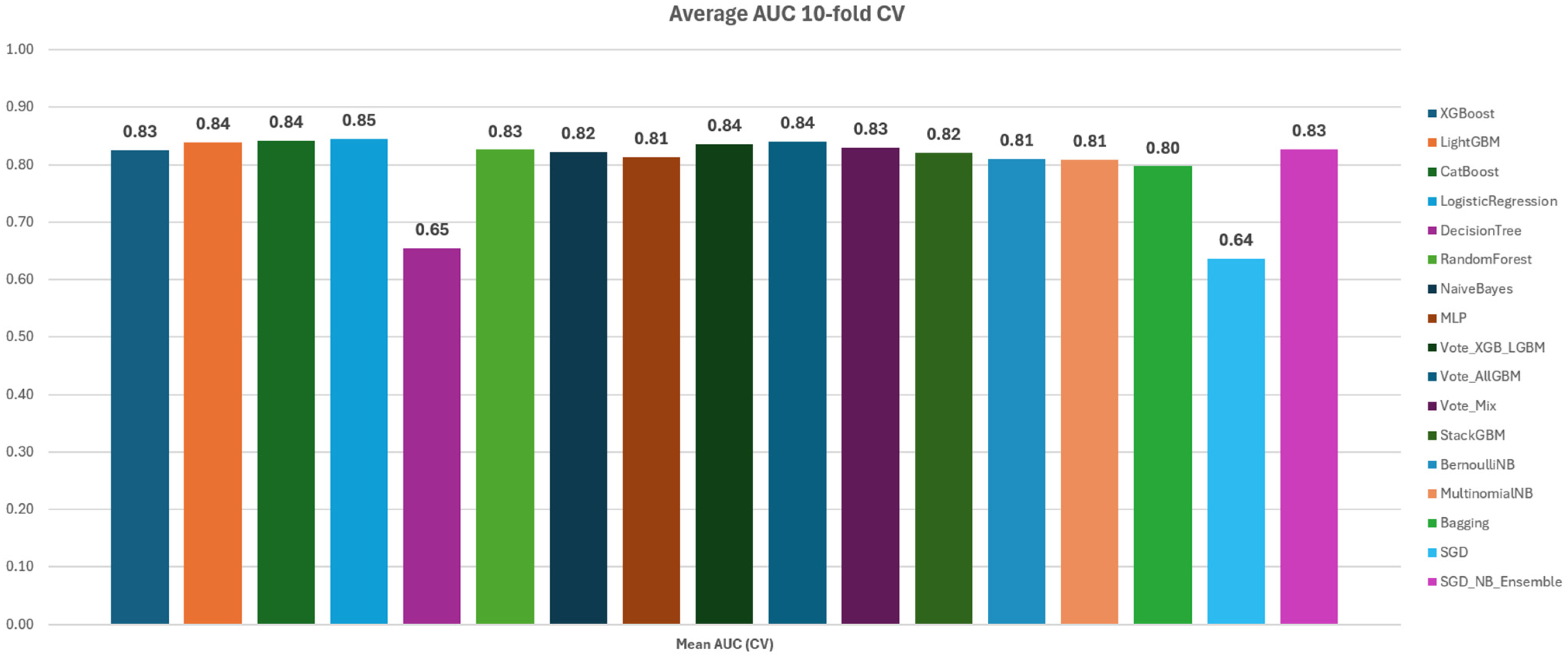
Figure 4 illustrates the corresponding AUC values for all ML models on the Telco dataset (10-fold CV). As it is observed, Logistic Regression achieved the highest AUC (0.85). The ML models Vote_AllGBM, Vote_XGB_LGBM, LightGBM and CatBoost reported an AUC of 0.84. Random Forest, Vote_Mix, MultinomialNB and SGD_NB_Ensemble showed an AUC of 0.83. Naïve Bayes, StackGBM and SGD achieved an AUC of 0.82 while MLP and BernoulliDB noted an AUC of 0.81. Bagging followed with an AUC of 0.80 and, finally, Decision Tree with an AUC of 0.65.

Figure 5 visualizes the results of the Log Loss values for the Telco dataset. Vote_XGB_LGBM achieved 0.44 Log Loss while Vote_AllGBM noted the lowest Log Loss of 0.43. Logistic Regression achieved 0.49 Log Loss, StackGBM had Log Loss of 0.5, while the rest of the ML models noted Log Loss values higher than 0.50 (Random Forest 0.51, MLP 0.55, MultinomialNB 0.82, SGD_NB_Ensemble 0.84, Bagging 1.31, BernoulliNB 1.09 and Naïve Bayes 2.88).

Interestingly, Logistic Regression achieved a good AUC of 0.85 and Log Loss of 0.49. The Telco dataset has many categorical features encoded with one-hot encoding that make it a good candidate for applying Logistic Regression. Based on the results of the Telco dataset, which are included in

Table 5. Evaluation metrics for 10-fold CV, on dataset Telco (PC).

ML Model	Mean Accuracy	Mean Precision	Mean Recall	Mean F1-Score	Mean AUC (CV)	Mean Log Loss (CV)
XGBoost	0.76	0.54	0.67	0.60	0.83	0.50
LightGBM	0.76	0.54	0.74	0.62	0.84	0.47
CatBoost	0.76	0.54	0.75	0.63	0.84	0.47
Logistic Regression	0.75	0.52	0.80	0.63	0.85	0.49
Decision Tree	0.73	0.50	0.48	0.49	0.65	9.53
Random Forest	0.79	0.63	0.47	0.54	0.83	0.51
Naïve Bayes	0.65	0.43	0.89	0.58	0.82	2.88
MLP	0.74	0.51	0.73	0.60	0.81	0.55
Vote_XGB_LGBM	0.80	0.65	0.52	0.58	0.84	0.44
Vote_AllGBM	0.80	0.65	0.51	0.57	0.84	0.43
Vote_Mix	0.77	0.57	0.63	0.60	0.83	0.47
StackGBM	0.79	0.62	0.49	0.55	0.82	0.50
BernoulliNB	0.67	0.44	0.87	0.58	0.81	1.09
MultinomialNB	0.73	0.50	0.79	0.61	0.83	0.82
Bagging	0.78	0.61	0.43	0.50	0.80	1.31
SGD	0.77	0.61	0.60	0.58	0.82	2.69
SGD_NB_Ensemble	0.75	0.54	0.72	0.61	0.83	0.84

, the ensemble approaches of Vote_AllGBM and Vote_XGB_LGBM seem more suitable for SaaS providers looking to obtain more reliable churn probabilities for their users and thus, targets users that are more likely to churn. However, those models “catch” fewer churners as opposed to models such as XGBoost, LightGBM, CatBoost and Logistic Regression, which showed better recall values (0.67, 0.74, 0.75 and 0.80, respectively), as shown in Table 5.

Therefore, SaaS providers that implement less expensive campaigns and are more concerned with not “missing” churners than targeting users that are more likely to churn, should prefer models such as XGBoost, LightGBM, CatBoost or even simpler models such as Logistic Regression.

3.1.2. Performance on Holdout

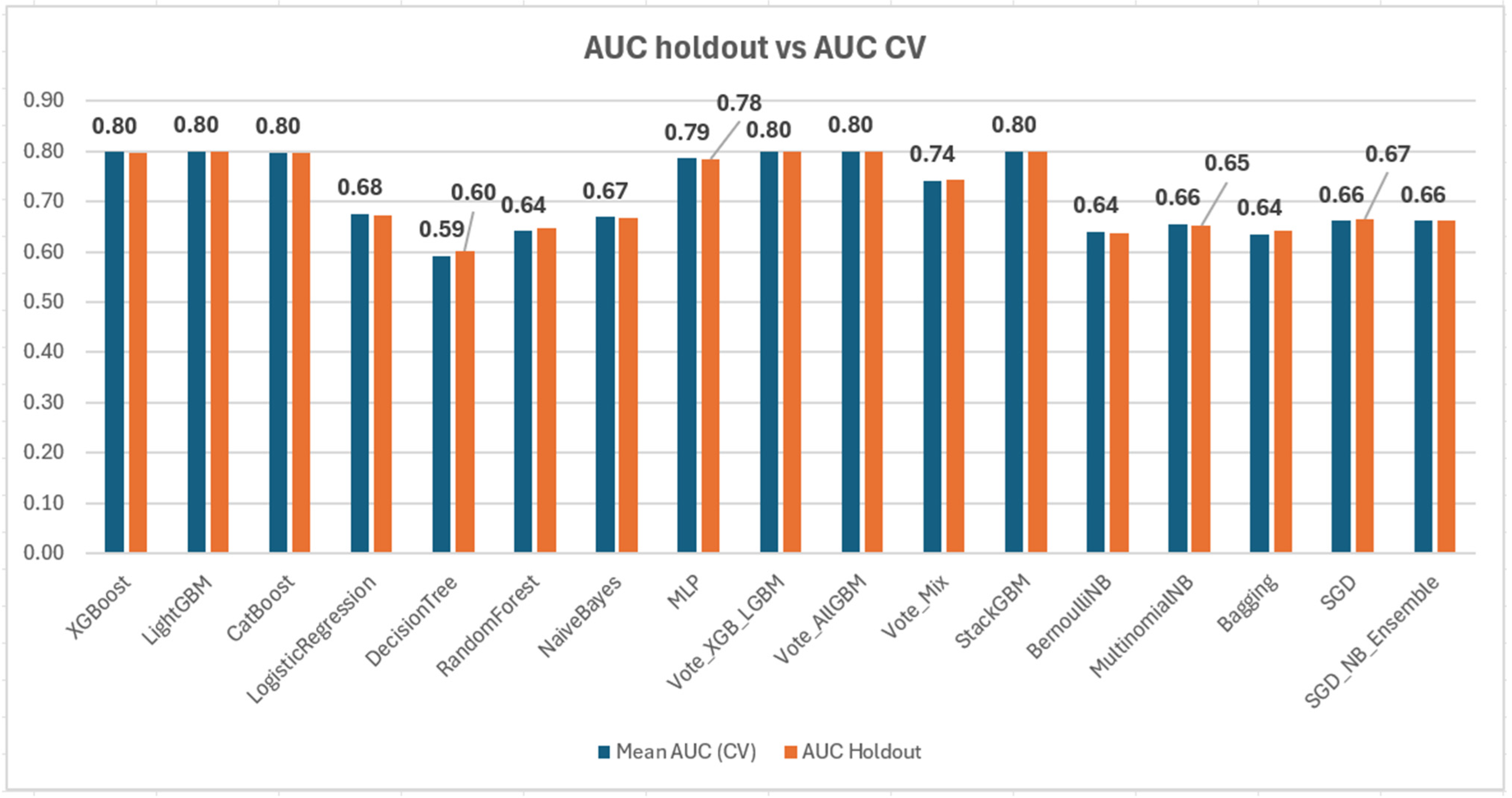
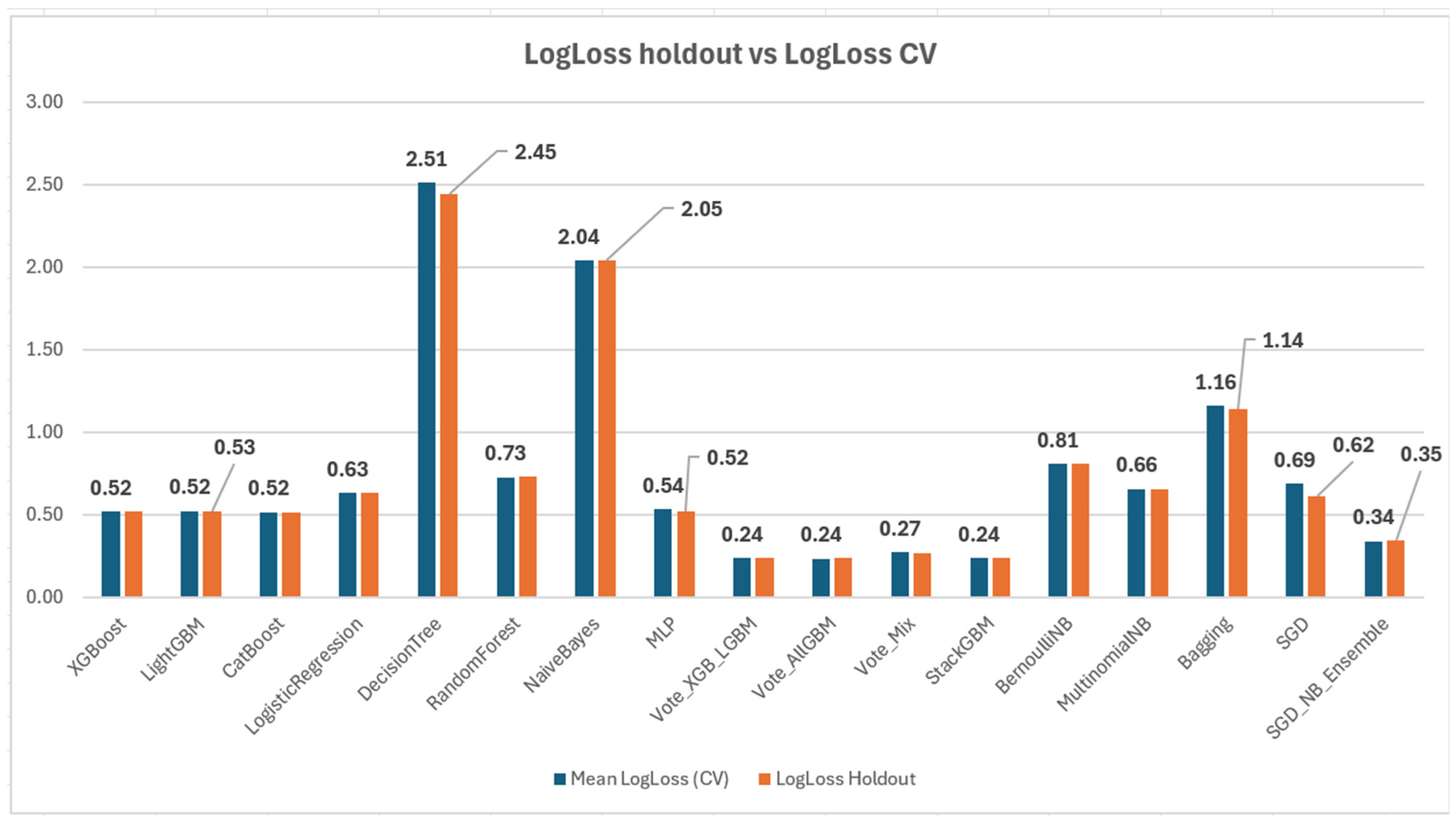
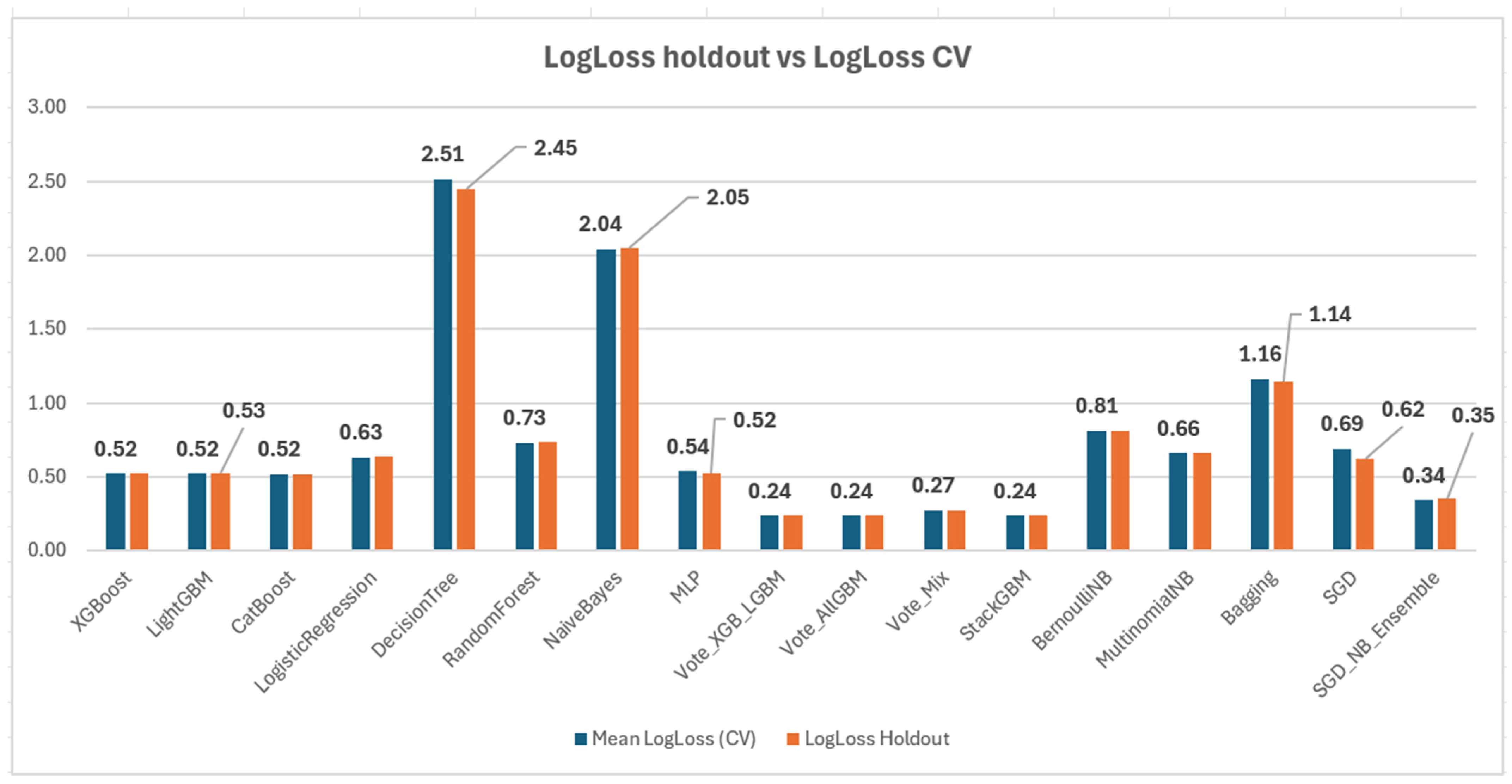
Comparing the evaluation results of the CV with the holdout evaluation results, there were noted small differences indicating that the cross-validation process was performed correctly and the ML models generalize well. Models with strong predictive performance showed tiny differences (≤0.01) while ML models with less predictive power noted larger differences such as Decision Tree, which achieved Log Loss of 2.51 in cross-validation and 2.45 in holdout showing a more unstable behavior due to their weak predictive performance (AUC 0.59–0.60). Figure 6 and Figure 7 illustrate AUC and Log Loss, respectively, for holdout versus CV for all models on the KKBOX dataset.

Similar were the results for the Telco dataset, as illustrated in Figure 8 and Figure 9. Most of the models noted almost identical evaluation metrics except ML models such as SDG and Decision Tree, which showed low predictive performance and more unstable behavior.

3.2. Efficiency Evaluation

3.2.1. Training Time on PC and Cloud

MLP and StackGBM required much more time to train compared to the rest of the models, as shown in Figure 10, illustrating the training time per ML model when performing 10-fold CV on the KKBOX dataset, running on PC. Specifically, MLP required 78.88 min, while similarly, StackGBM noted 76.43 min on the same settings. The rest of the ML models required less than half of the time spent on MLP and StackGBM. Specifically, Logistic Regression required 11.36 min, CatBoost 6.48 min, Random Forest 8.61 min and Vote_Mix 6.70 min. Bagging training needed 2.51 min and SGD 1.87 min. The rest of the ML models (XGBoost, LightGBM, Decision Tree, Vote_XGB_LGBM, BernoulliNB, MultinomialNB and SGD_NB_Ensemble) reported training times less than 1 min.

Similarly, when training the models on the cloud, the training time for MLP and StackGBM were quite larger than the rest of the models. As shown in

Table 6. Training time (min) for 10-fold CV, on dataset KKBOX (Google Cloud VMs).

Model	VM1	VM2	VM3	Average	Standard Deviation
XGBoost	0.42	0.41	0.43	0.42	0.01
LightGBM	0.47	0.47	0.48	0.47	0.00
CatBoost	8.57	8.50	9.23	8.77	0.33
Logistic Regression	13.53	12.95	15.41	13.96	1.05
Decision Tree	0.36	0.36	0.40	0.38	0.02
Random Forest	7.58	7.40	8.46	7.82	0.46
Naïve Bayes	0.15	0.14	0.16	0.15	0.01
MLP	101.49	102.13	102.76	102.13	0.52
Vote_XGB_LGBM	0.86	0.85	0.92	0.87	0.03
Vote_AllGBM	8.91	8.88	9.82	9.21	0.44
Vote_Mix	7.71	7.56	9.15	8.14	0.72
StackGBM	84.25	83.56	93.06	86.96	4.33
BernoulliNB	0.18	0.16	0.19	0.17	0.01
MultinomialNB	0.12	0.10	0.12	0.12	0.01
Bagging	2.26	2.24	2.54	2.34	0.14
SGD	2.17	2.07	2.90	2.38	0.37
SGD_NB_Ensemble	0.83	0.79	1.09	0.90	0.13

, MLP noted the larger training time of 102.13 min on average on the three Google Cloud VMs we used in the experiments. StackGBM followed with 86.96 min on average. Logistic Regression required 13.96 min and Vote_AllGBM 9.21 min The rest of the ML models required less than 10 min to train. In particular, CatBoost, Random Forest and Vote_Mix required 8.77, 7.82 and 8.14 min, respectively. Bagging training lasted 2.34 min. Extremely fast ML models with less than 1 min to train were Vote_XGB_LGBM (0.87 min), LightGBM (0.47 min), XGBoost (0.42 min), Decision Tree (0.38 min), SGD (0.37 min), BernoulliNB (0.17 min), SGD_Ensemble (0.13 min) and MultinomialNB (0.12 min).

Training times for the Telco dataset, visualized in Figure 11, were much smaller compared to KKBOX, as expected, since it is a much smaller dataset. However, there were still notable differences among the models. StackGBM had the highest training time of 105.15 s. MLP was next with 34.89 s. Vote_AllGBM followed with 16.61 s and CatBoost with 13.67. Random Forest and Vote_Mix noted 4.37 and 2.32 s, respectively. Vote_XGM_LGBM’s training lasted 2.08 s. XGBoost and Logistic Regression were very fast, noting training times less than 2 s (1.34 s and 1.27 s, respectively). LightGBM was even faster to train, noting 0.91 s of training time quite close to and SGD_NB_Ensemble (0.95 s). The fastest to train were the simpler models like SGD (0.63 s), Decision Tree (0.36 s), Naïve Bayes (0.16 s), BernoulliNB (0.18 s) and MultinomialNB (0.15 s).

Table 7. Training time (seconds) for 10-fold CV, on the Telco dataset (Google Cloud VMs).

Model	VM1	VM2	VM3	Average	Standard Deviation
XGBoost	0.75	0.76	0.78	0.77	0.01
LightGBM	0.74	0.74	0.77	0.75	0.01
CatBoost	18.14	18.12	18.50	18.25	0.17
Logistic Regression	0.84	0.84	0.89	0.86	0.02
Decision Tree	0.33	0.33	0.34	0.33	0.00
Random Forest	4.61	4.60	4.68	4.63	0.04
Naïve Bayes	0.12	0.12	0.13	0.12	0.01
MLP	26.89	26.60	26.67	26.72	0.12
Vote_XGB_LGBM	1.54	1.54	1.57	1.55	0.01
Vote_AllGBM	19.09	19.12	19.51	19.24	0.19
Vote_Mix	2.29	2.18	2.22	2.23	0.05
StackGBM	128.47	128.17	130.69	129.11	1.12
BernoulliNB	0.14	0.14	0.13	0.14	0.00
MultinomialNB	0.11	0.11	0.11	0.11	0.00
Bagging	1.69	1.69	1.71	1.69	0.01
SGD	0.49	0.50	0.49	0.49	0.00
SGD_NB_Ensemble	0.77	0.78	0.77	0.77	0.00

summarizes the training time for each ML model when performing 10-fold CV on Google Cloud VMs. StackGBM showed the largest training time compared to the rest of the ML models (129.11 s). MLP followed with 26.72 s, Vote_AllGBM with 19.24 s and CatBoost with 18.25 s. Random Forest, Vote_Mix and Vote_XGB_LGBM noted training times of 4.62, 2.23 and 1.55 s, respectively. Extremely fast training with less than 1 s was noted in the case of XGBoost (0.77 s), SGD_NB_Ensemble (0.77 s), LightGBM (0.75 s), SGD (0.49 s), Decision Tree (0.33 s), Naïve Bayes (0.12 s), BernoulliNB (0.14 s) and MultinomialNB (0.11 s).

3.2.2. Prediction Time, Mean Latency and Throughput on the Cloud

The training time of ML models is important, yet, in order to efficiently use a model in real-time production, it is important to also consider other factors such the time needed for generating predictions. For that reason, we conducted another set of experiments in the three VMs where we trained the ML models in the 80% train set, saved that model in the VM and called it for generating predictions for the holdout set (the remaining 20%). The following metrics are calculated for each model:

• Total prediction time for the complete holdout set.
• Mean Latency, referring to the time needed for generating prediction for one sample.
• Throughput, as the number of predictions per second.

Table 8. Prediction time, Mean Latency and Throughput metrics on different VMs for 10-fold CV, on the KKBOX dataset.

VM- Region	VM1: Asia -Northeast1-b 19:00 UTC			VM2: EU—West3 19:00 UTC			VM3: US West1 19:00 UTC			Average
Model	Prediction Time (s)	Mean Latency (ms)	Throughput (Sample/s)	Prediction Time (s)	Mean Latency (ms)	Throughput (Sample/s)	Prediction Time (s)	Mean Latency (ms)	Throughput (Sample/s)	Prediction Time (s)	Mean Latency (ms)	Throughput (Sample/s)
XGBoost	0.26	0.0014	734,685	0.26	0.0014	738,269	0.27	0.0014	7,173,49	0.27	0.0014	730,101
LightGBM	0.72	0.0037	268,879	0.72	0.0037	271,588	0.73	0.0037	267,240	0.72	0.0037	269,236
CatBoost	0.15	0.0008	1,289,414	0.15	0.0008	1,279,011	0.15	0.0008	1,282,835	0.15	0.0008	1,283,753
Logistic Regression	0.04	0.0002	5,544,422	0.03	0.0002	5,779,359	0.04	0.0002	4,831,150	0.04	0.0002	5,384,977
Decision Tree	0.12	0.0006	1,571,370	0.12	0.0006	1,652,179	0.15	0.0008	1,314,524	0.13	0.0007	1,512,691
Random Forest	8.36	0.0430	23,230	8.42	0.0433	23,076	9.44	0.0486	20,566	8.74	0.0450	222,91
Naïve Bayes	0.20	0.0010	956,918	0.20	0.0010	973,352	0.30	0.0015	650,896	0.23	0.0012	860,389
MLP	0.75	0.0039	259,671	0.72	0.0037	268,738	0.81	0.0042	240,661	0.76	0.0039	256,357
Vote_XGB_LGBM	0.96	0.0049	202,767	0.94	0.0049	205,789	0.98	0.0050	198,943	0.96	0.0049	202,500
Vote_AllGBM	1.08	0.0055	180,425	1.06	0.0055	182,626	1.11	0.0057	175,146	1.08	0.0056	179,399
Vote_Mix	0.61	0.0031	319,971	0.59	0.0030	330,234	0.69	0.0036	281,362	0.63	0.0032	310,522
StackGBM	9.78	0.0504	19,854	9.85	0.0507	19,711	10.88	0.0561	17,840	10.17	0.0524	19,135
BernoulliNB	0.30	0.0015	648,956	0.30	0.0015	656,327	0.41	0.0021	477,180	0.33	0.0017	594,154
MultinomialNB	0.18	0.0009	1,084,657	0.18	0.0009	1,062,531	0.26	0.0013	750,543	0.21	0.0011	965,910
Bagging	1.06	0.0055	183,303	1.05	0.0054	185,121	1.37	0.0070	141,957	1.16	0.0060	170,127
SGD	0.03	0.0002	5,623,307	0.03	0.0002	6,072,912	0.04	0.0002	4,569,442	0.04	0.0002	5,421,887
SGD_NB_Ensemble	0.21	0.0011	938,350	0.19	0.0010	1,024,291	0.28	0.0014	699,297	0.22	0.0012	887,313

contains the prediction metrics for each ML model and their average values across all VMs, on the KKBOX dataset. Results are almost identical for different regions for the same ML model and the marginal differences can be due to other reasons as well, ML models can slightly vary even when trained on the same data and same conditions. However, there are notable differences among the prediction metrics for each ML model. As shown in Figure 12, StackGBM and Random Forest have much higher Mean Latency compared to the rest of the models (0.0524 ms and 0.045 ms, respectively). Bagging followed with 0.0060 ms, VoteAllGBM with 0.0056 ms and Vote_XGB_LGBM with 0.0049 ms. MLP came next with 0.0039 ms, LightGBM with 0.0037 ms and Vote_Mix with 0.0032 ms. CatBoost and XGBoost were even faster, noting values of 0.008 ms and 0.0014, outperforming simpler models like BernoulliNB (0.0017 ms). CatBoost outperformed even Naïve Bayes and MultinomialNB which achieved a Mean Latency of 0.0012 ms and 0.0011 ms, respectively. Similarly, SGD_NB_Ensemble noted a value of 0.0012 ms. The fastest ones where Logistic Regression and SGD with 0.0002 ms followed by the Decision Tree which noted 0.0006 ms of Mean Latency.

The same conclusions regarding how fast the ML models are on inference can be drawn when looking at the total prediction time, since it is the Mean Latency multiplied by the number of instances on the holdout set. The same stands for Throughput. As shown in Table 8, fast models like CatBoost can provide predictions for more than 1 million records in a second, and simple models like Logistic Regression and Decision Tree can give predictions for more almost 10× million records in one second. On the contrary, models such as StackGBM and Random Forest can predict on average 19.135 and 22.291 instances per second, respectively. This is an important aspect to consider when using those ML models in production, since for SaaS providers with many users, this can cause delays if they use the ML models frequently. So, ML models like StackGBM and Random Forest are not among the best options if the models are meant to be used frequently. Complementary Figure 12 visualizes the Mean Latency (ms) in VMs (average on regions) for all models, on the KKBOX dataset.

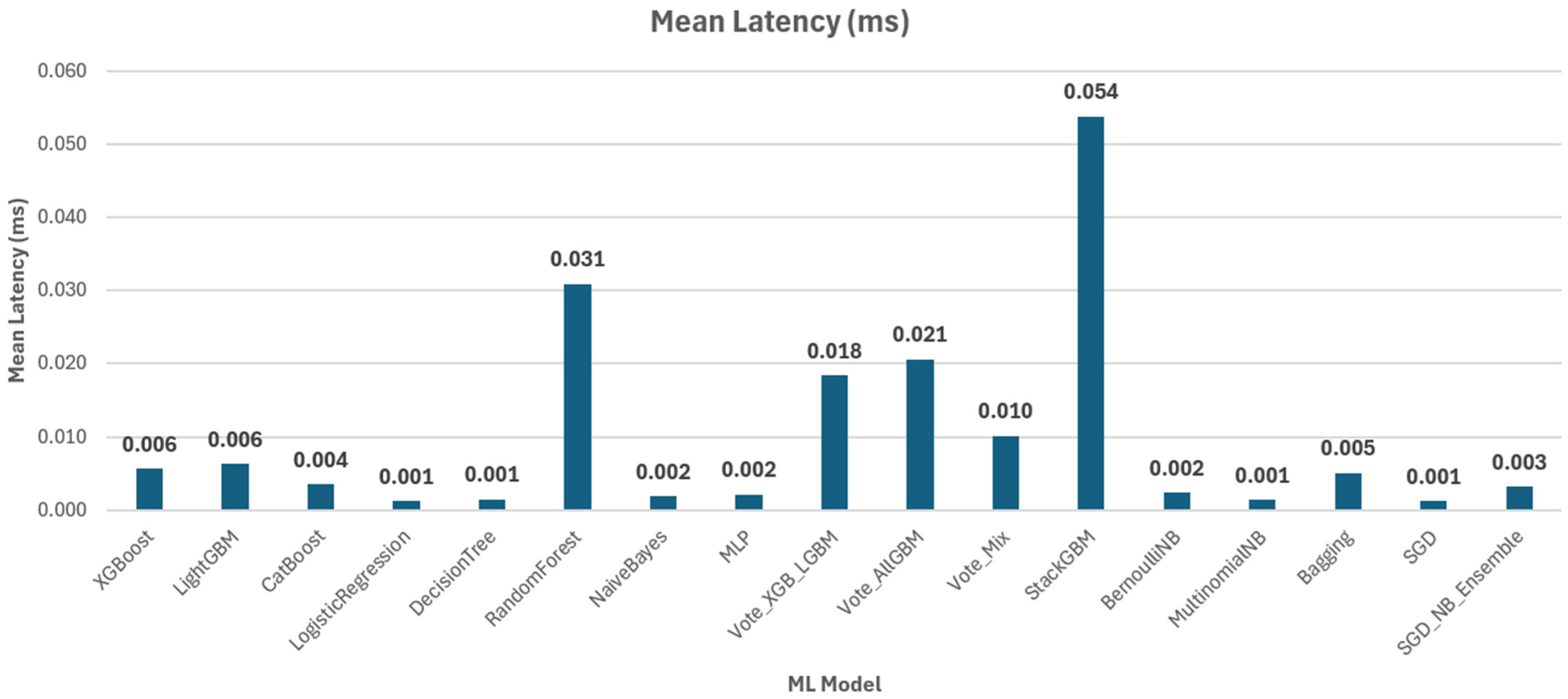
Smaller prediction times were witnessed for the Telco dataset, which was as expected due to its small size. However, there are still differences among the ML models’ prediction times. The relative difference among the prediction time of models is similar to the ones noted for the KKBOX dataset.

Table 9. Prediction time, Mean Latency and Throughput metrics on different VMs for 10-fold CV, on the Telco dataset.

VM- Region	VM1: Asia -Northeast1-b 19:00 UTC			VM2: EU—West3 19:00 UTC			VM3: US West1 19:00 UTC			Average
Model	Prediction Time (s)	Mean Latency (ms)	Throughput (Sample/s)	Prediction Time (s)	Mean Latency (ms)	Throughput (Sample/s)	Prediction Time (s)	Mean Latency (ms)	Throughput (Sample/s)	Prediction Time (s)	Mean Latency (ms)	Throughput (Sample/s)
XGBoost	0.0079	0.0056	178,923	0.0078	0.0056	180,002	0.0081	0.0058	173,669	0.0079	0.0056	177,532
LightGBM	0.0088	0.0063	159,260	0.0087	0.0062	161,350	0.0089	0.0063	157,521	0.0088	0.0063	159,377
CatBoost	0.0050	0.0035	282,768	0.0047	0.0033	302,419	0.0053	0.0038	264,270	0.0050	0.0035	283,152
Logistic Regression	0.0017	0.0012	829,499	0.0016	0.0011	872,892	0.0017	0.0012	822,225	0.0017	0.0012	841,539
Decision Tree	0.0020	0.0014	695,009	0.0019	0.0014	727,719	0.0021	0.0015	685,792	0.0020	0.0014	702,840
Random Forest	0.0430	0.0305	32,787	0.0421	0.0299	334,56	0.0455	0.0323	30,939	0.0435	0.0309	32,394
Naïve Bayes	0.0025	0.0018	556,942	0.0025	0.0018	561,396	0.0027	0.0019	516,470	0.0026	0.0018	544,936
MLP	0.0031	0.0022	449,947	0.0027	0.0019	523,212	0.0031	0.0022	460,401	0.0030	0.0021	477,853
Vote_XGB_LGBM	0.0245	0.0174	57,597	0.0264	0.0188	53,283	0.0267	0.0190	52,724	0.0259	0.0184	54,534
Vote_AllGBM	0.0316	0.0224	44,575	0.0280	0.0198	50,403	0.0277	0.0196	50,956	0.0291	0.0206	48,645
Vote_Mix	0.0142	0.0101	99,065	0.0138	0.0098	102,061	0.0148	0.0105	95,424	0.0143	0.0101	98,850
StackGBM	0.0792	0.0562	17,793	0.0740	0.0525	19,035	0.0743	0.0527	18,958	0.0758	0.0538	18,595
BernoulliNB	0.0034	0.0024	418,840	0.0032	0.0023	436,877	0.0036	0.0025	395,853	0.0034	0.0024	417,190
MultinomialNB	0.0020	0.0014	713,098	0.0020	0.0014	720,366	0.0020	0.0015	688,440	0.0020	0.0014	707,301
Bagging	0.0070	0.0049	202,235	0.0069	0.0049	203,858	0.0074	0.0053	189,930	0.0071	0.0050	198,674
SGD	0.0016	0.0012	861,509	0.0016	0.0011	874,215	0.0018	0.0013	796,528	0.0017	0.0012	844,084
SGD_NB_Ensemble	0.0045	0.0032	315,807	0.0044	0.0031	319,760	0.0047	0.0034	297,607	0.0045	0.0032	311,058

includes the prediction time metrics for all VMs and models, while Figure 13 illustrates the Mean Latency (ms) in VMs (average on regions) for all models, on the Telco dataset.

The fastest ML models were Logistic Regression, Decision Tree, MultinomialNB and SGD with 0.001 ms Mean Latency. MLP, Naïve Bayes and BernoulliNB achieved 0.002 ms Mean Latency. SGD_NB_Ensemble was fast with 0.003 ms Mean Latency followed by CatBoost with 0.004 ms. Bagging was the next fastest with 0.005 ms followed by XGBoost and LightGBM, which achieved 0.006 ms Mean Latency. The voting schemes Vote_XGB_LGBM, VoteAllGBM and Vote_Mix achieved 0.018, 0.021 and 0.010 ms, respectively. StackGBM was again the slowest at 0.054 ms followed by Random Forest and Multinomial NB with 0.02 ms.

3.3. Sustainability Evaluation

3.3.1. Energy and Emissions on PC

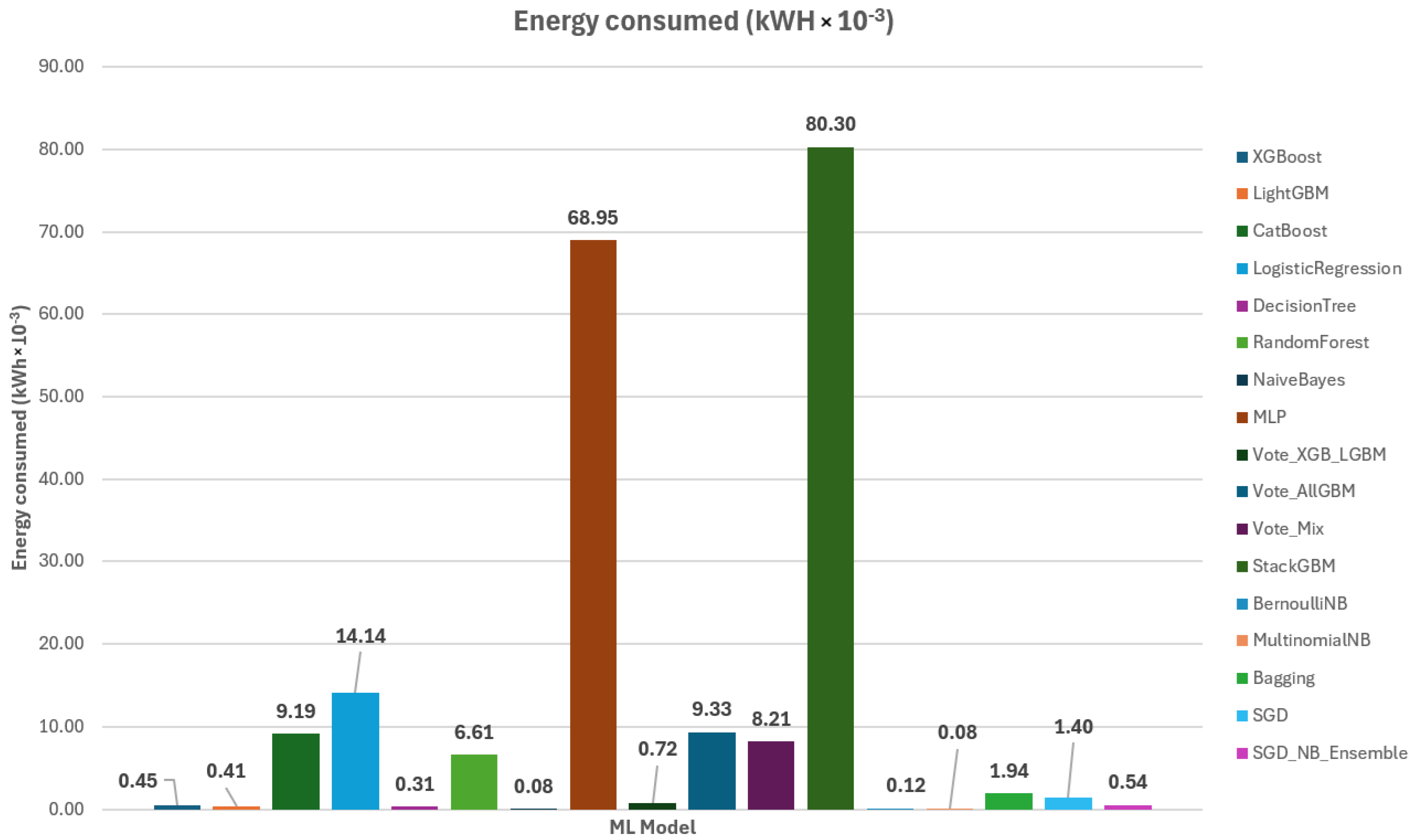
Figure 14 presents the total energy consumption for a 10-fold CV on the KKBOX dataset when running on a PC as measured by the CodeCarbon library, taking into account the geographical region as detected by the IP address. The experiments took place in Kavala, Greece. The highest energy consumption was noted by the ML model StackGBM (80.30 × 10⁻³ kWh). In similar levels, MLP consumed 68.95 × 10⁻³ kWh. The rest of the ML models consumed a smaller amount of energy. In particular, Logistic Regression required 14.4 × 10⁻³ kWh, CatBoost required 9.19 × 10⁻³ kWh, Vote_AllGBM required 9.33 × 10⁻³ kWh, Vot_Mix required 8.21 × 10⁻³ kWh and Random Forest required 6.61 × 10⁻³ kWh. The rest of the ML models consumed lower levels of energy. Specifically, XGBoost consumed 0.45 × 10⁻³ kWh, LightGBM consumed 0.41 × 10⁻³ kWh, Vote_XGB_LGBM consumed 0.72 × 10⁻³ kWh, Bagging consumed 1.94 × 10⁻³ kWh and Vote_Mix (1.13 × 10⁻³ kWh) and SGD (0.54 × 10⁻³ kWh). Even smaller levels of consumed energy were noted for Decision Tree (0.31 × 10⁻³ kWh), Naïve Bayes (0.08 × 10⁻³ kWh), BernoulliNB (0.12 × 10⁻³ kWh), MultinomialNB (0.08 × 10⁻³ kWh) and SGD_NB_Ensemble (0.54 × 10⁻³ kWh).

For the Telco dataset (Figure 15), the levels of energy consumption were much less than in the KKBOX dataset since it is much smaller, and the ML models completed training very quickly. However, there were still notable differences among the energy consumption levels that different ML models required and are relatively similar to the consumption levels noted for the KKBOX dataset, with the exception of Logistic Regression, which had the third highest energy consumption for KKBOX but a very low value for the Telco dataset. The Telco dataset has only 5634 training records (7043 total). On the contrary, the KKBOX dataset is almost 100× times the size of the Telco, with a training set of 551.401 records (745.593 total). So Logistic Regression’s training lasted longer than in KKBOX since it had many more training records to process. StackGBM consumed the highest level of energy of 2.179 × 10⁻³ kWh. The next highest values were noted by MLP, CatBoost, and VoteAllGBM (0.539, 0.298 and 0.366 × 10⁻³ kWh). Random Forest came next with 0.056 × 10⁻³ kWh, Vote_Mix with 0.046 × 10⁻³ kWh, Vote_XGB_LGBM with 0.046 × 10⁻³ kWh and Bagging with 0.025 × 10⁻³ kWh. The rest of the ML models followed with even less energy consumption. Specifically, XGBoost and Logistic Regression noted 0.026 × 10⁻³ kWh, followed by LightGBM with 0.018 × 10⁻³ kWh. The least amount of energy consumption (0.002 × 10⁻³ kWh) was noted by Naïve Bayes and MultinomialNB. Slightly higher values of consumed energy were shown by BernoulliNB (0.003 × 10⁻³ kWh), Decision Tree (0.005 × 10⁻³ kWh), SGD (0.008 × 10⁻³ kWh) and SGD_NB_Ensemble (0.012 × 10⁻³ kWh).

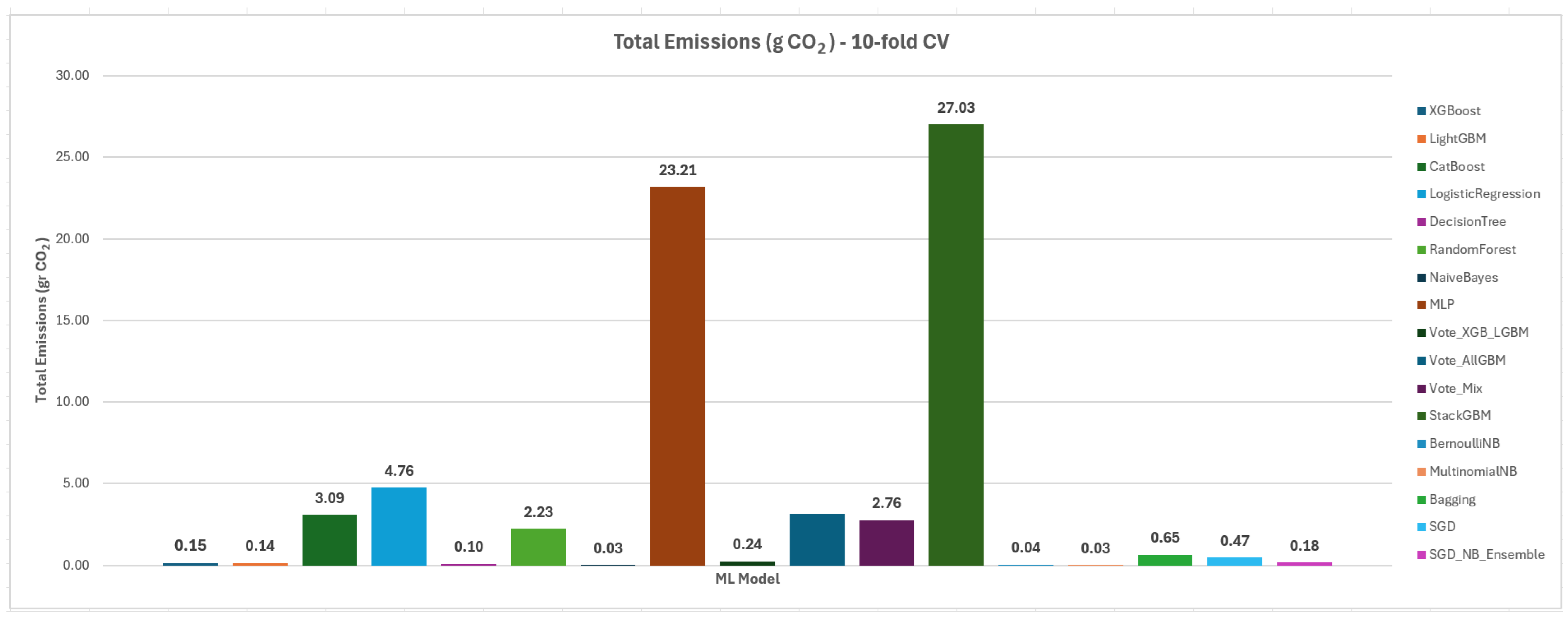
Figure 16 presents the emissions generated when training the ML models on a 10-fold CV on PC for the KKBOX dataset. As expected, the ML models that required more time to complete the training generated higher levels of emissions. CO₂ emissions and energy consumption are interrelated. Cloud computing and ML workloads consume electricity, resulting in CO₂ emissions, this also depends on the energy mix of the grid (coal-powered grid, renewable-powered grid). The evaluation of ML models should therefore also be based on energy and emissions data, in the steps towards identifying eco-friendly options. StackGBM generated the highest value of emissions (27.03 g CO₂) compared to the rest of the ML models. MLP followed at similar levels with a value of 23.21 g CO₂. The rest of the ML models noted much less emissions ranging from 4.76 g CO₂ for Logistic Regression to 0.02 g CO₂ for Naïve Bayes and MultinomialNB.

Similarly, for the Telco dataset (Figure 17) the emissions generated were much higher for MLP and StackGBM than for the rest of the ML models. Thus, the highest emissions were generated by StackGBM (73.36 × 10⁻² g CO₂). MLP came next with 18.13 × 10⁻² g CO₂, while the smallest values of generated emissions were noted by the Bayes models (Naïve Bayes 0.07 × 10⁻² g CO₂, BernoulliNB 0.09 × 10⁻² g CO₂, MultinomialNB × 10⁻² g CO₂) followed by Decision Tree (0.16 × 10⁻² g CO₂) and SGD (0.29 × 10⁻² g CO₂).

In the case of the Telco dataset, energy consumption values as well as emissions are small for all models, yet with relative differences. Given the fact that those processes run repeatedly and by many different SaaS providers, their cumulative effect across runs results in negligible values to add up, leading to non-trivial energy consumption and emissions at scale. Moreover, the actual values increase as the size of the datasets increases; the values for the KKBOX dataset are much higher compared to the respective ones for the Telco dataset. Moreover, it should also be considered that, based on SaaS providers’ business policy, churn prediction models are trained and called for inference frequently, so as to be updated with new data, aggregating in a meaningful carbon footprint.

3.3.2. Energy and Emissions on the Cloud

The same training process was also followed for the three Google Cloud VMs with the exact same specifications and settings, yet in a different geographical region. The aim of this experiment is to compare the generated emissions when training ML models in different regions.

The emissions generated on the cloud are less for all ML models, compared to the corresponding emissions generated when the models run on the PC, although a one-to-one comparison is not valid since the PC machine does not have the same specifications as the VMs.

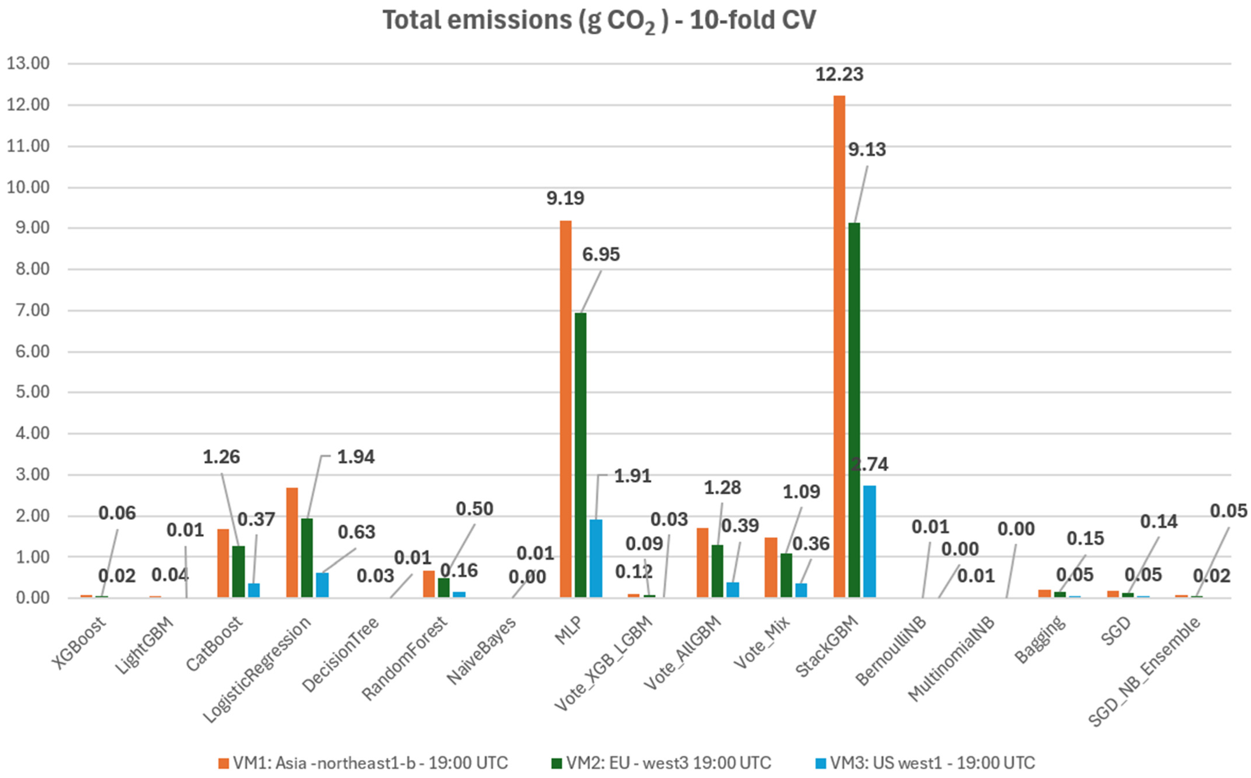
Figure 18 contains the emissions generated per ML model when running on the three Google Cloud VMs for the KKBOX dataset. For all the ML models, the emissions generated when running in VM1 of the Asia-northeast1-b region were found to be higher compared to those of the other two regions. On the contrary, the emissions generated in the US-west1 region were the lowest when compared to the emissions generated in the other regions. As is presented in

Table 10. Total emissions (g CO₂) in different regions for 10-fold CV, on the KKBOX dataset.

Model	VM1	VM2	VM3	Emission VM1/ Emissions VM2	Emission VM2/ Emissions VM3	Emission VM1/ Emissions VM3
XGBoost	0.08	0.06	0.02	1.34	3.56	4.78
LightGBM	0.05	0.04	0.01	1.35	3.61	4.87
CatBoost	1.69	1.26	0.37	1.34	3.37	4.53
Logistic Regression	2.69	1.94	0.63	1.39	3.09	4.29
Decision Tree	0.03	0.03	0.01	1.34	3.31	4.43
Random Forest	0.69	0.50	0.16	1.36	3.21	4.38
Naïve Bayes	0.01	0.01	0.00	1.40	3.17	4.43
MLP	9.19	6.95	1.91	1.32	3.65	4.82
Vote_XGB_LGBM	0.12	0.09	0.03	1.35	3.38	4.55
Vote_AllGBM	1.71	1.28	0.39	1.33	3.31	4.42
Vote_Mix	1.47	1.09	0.36	1.35	3.03	4.10
StackGBM	12.23	9.13	2.74	1.34	3.33	4.46
BernoulliNB	0.02	0.01	0.00	1.43	3.19	4.55
MultinomialNB	0.01	0.01	0.00	1.54	3.10	4.77
Bagging	0.20	0.15	0.05	1.34	3.24	4.34
SGD	0.20	0.14	0.05	1.39	2.63	3.66
SGD_NB_Ensemble	0.08	0.05	0.02	1.41	2.69	3.79

, the emissions generated in the VM1 region were 3.66× to 4.87× times higher than the emissions generated in the VM3 region. By comparing the emissions generated when training the models on VM2 and VM3, we noticed that the emissions generated for all models were more than 2.5× times higher than in VM3, ranging from 2.63 for SGD to 3.65 for MLP. Lastly, when comparing the emissions generated by the ML models in VM1 and VM2, we noticed that VM1 emissions were 1.32× to 1.54× times the emissions in VM2 for all ML models.

Table 11. Total emissions (g × 10⁻² CO₂) in different regions for 10-fold CV, on the Telco dataset.

Model	VM1	VM2	VM3	Emission VM1/ Emissions VM2	Emission VM2/ Emissions VM3	Emission VM1/ Emissions VM3
XGBoost	0.20	0.15	0.04	1.32	3.54	4.68
LightGBM	0.19	0.14	0.04	1.32	3.58	4.74
CatBoost	5.92	4.45	1.22	1.33	3.63	4.83
Logistic Regression	0.27	0.20	0.06	1.35	3.18	4.28
Decision Tree	0.12	0.09	0.03	1.34	3.64	4.87
Random Forest	0.77	0.58	0.16	1.33	3.61	4.81
Naïve Bayes	0.09	0.07	0.02	1.33	3.60	4.79
MLP	4.18	3.11	0.85	1.35	3.66	4.93
Vote_XGB_LGBM	0.36	0.27	0.08	1.34	3.57	4.78
Vote_AllGBM	6.04	4.54	1.23	1.33	3.69	4.91
Vote_Mix	0.74	0.54	0.15	1.37	3.62	4.97
StackGBM	36.73	27.50	7.69	1.34	3.58	4.78
BernoulliNB	0.10	0.07	0.02	1.33	3.68	4.89
MultinomialNB	0.09	0.07	0.02	1.33	3.67	4.87
Bagging	0.33	0.25	0.07	1.33	3.64	4.83
SGD	0.15	0.11	0.03	1.33	3.69	4.89
SGD_NB_Ensemble	0.19	0.14	0.04	1.32	3.70	4.88

contains the emissions generated when performing a 10-fold CV on the Telco dataset on the three VMs. Although the emissions are much less compared to when training on the KKBOX dataset, there are still noted differences when training on different regions. The emissions generated when training on VM1 were 4.28× to 4.97× times higher than the emissions generated on VM3. In comparison with the emissions generated when training on VM2, we noticed 3.18× to 3.70× times higher emissions than the emissions generated when training on VM3, as shown in Table 9. Finally, when comparing the emissions of VM1 to those of VM2, we reported 1.32× to 1.37× times higher emissions for all the ML models.

3.3.3. Models’ Size

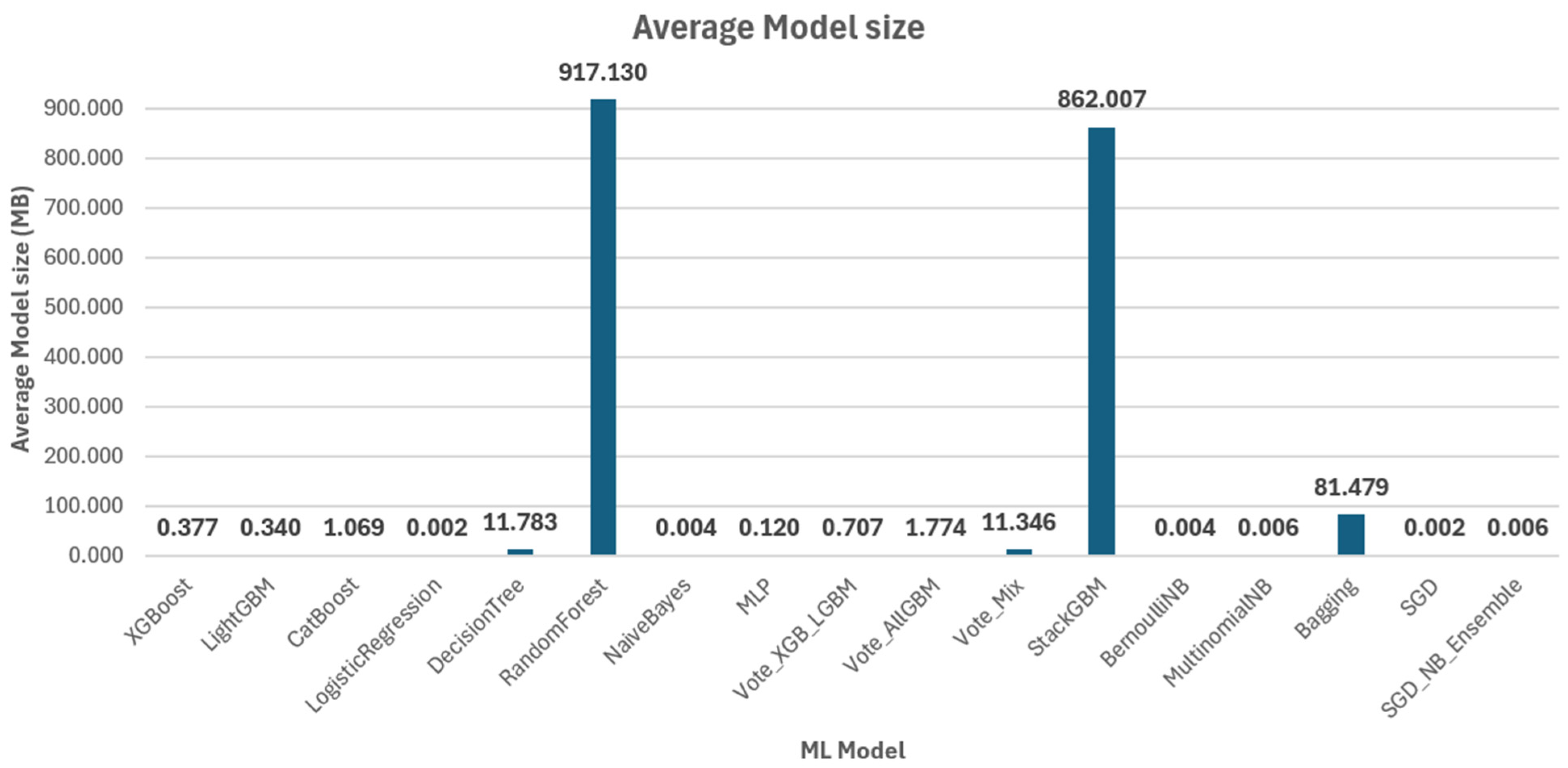
Another interesting aspect to consider for the efficient use and sustainability of the ML models for SaaS decision support is their size. Large models are harder to maintain in the cloud since they require more space to be saved. It is important to notice that the models that were the slowest at inference (StackGBM and Random Forest) showed to have the largest model size. As is shown in Figure 19 regarding the KKBOX dataset, the slowest models, StackGBM and Random Forest, had the largest sizes of 862.007 mb and 917.13 mb, respectively. The next largest model was generated by Bagging (81.479 mb). The Decision Tree model was 11.783 mb and Vote_Mix 11.346 mb. Vote_AllGBM’s size was 1.774 mb and CatBoost’s size was 1.069 mb. The rest of the models had sizes less than 1 mb.

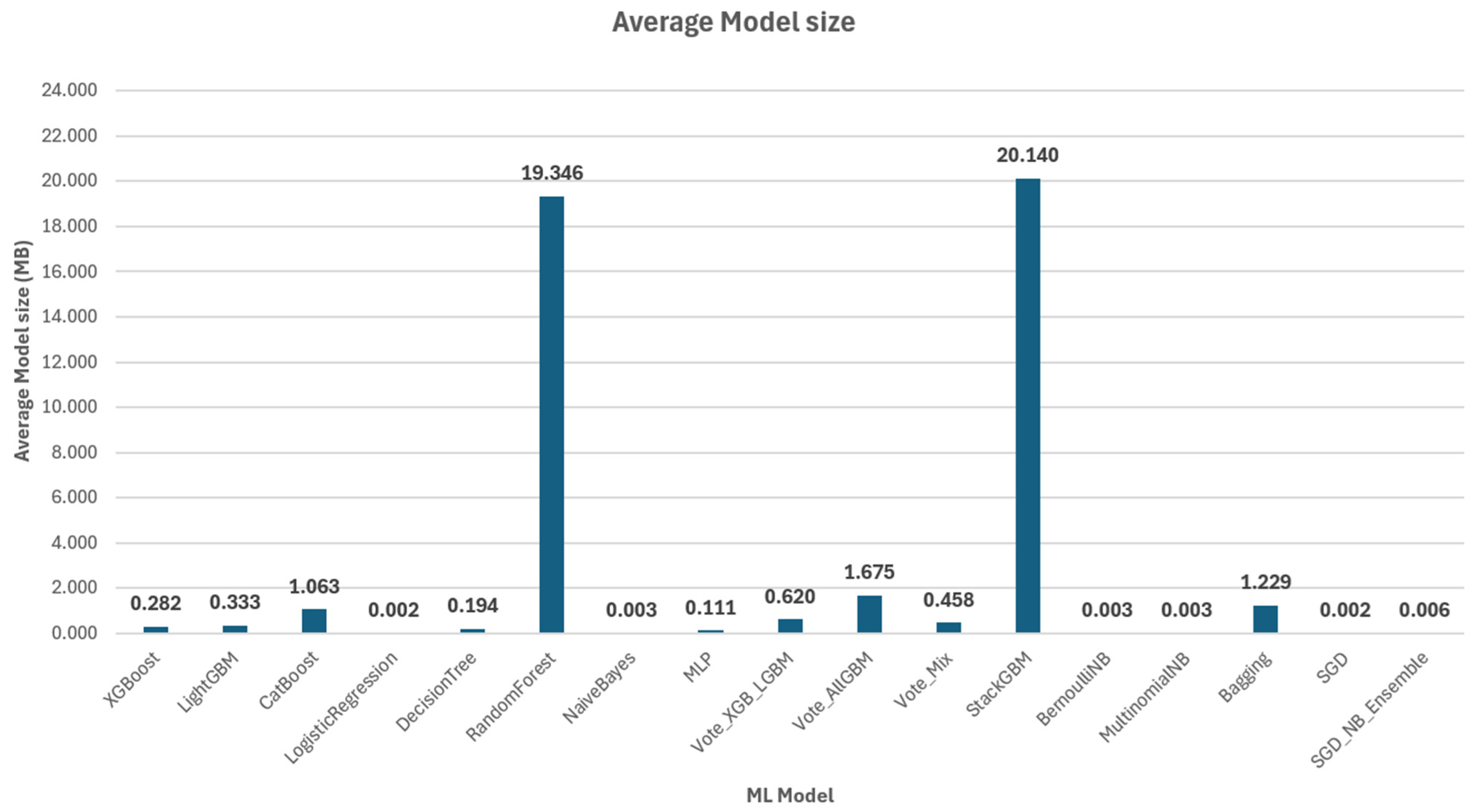
Similarly, for the Telco dataset (Figure 20), the largest models in size were the slowest ones, namely StackGBM (20.140 mb) and Random Forest (19.346 mb), as shown in Figure 20. Vote_AllGBM model’s size was 1.675 mb, Bagging’s was 1.229 mb, and CatBoost’s was 1.069 mb. The rest of the ML models had sizes less than 1 mb.

3.4. Overall Evaluation

3.4.1. Pareto Frontiers Analysis

In order to select an ML model supporting SaaS providers, multiple objectives should be considered. Predictive performance is undoubtedly important. However, objectives like emissions, training time and latency of the ML models should also be considered to have a sustainable and efficient solution to be used in production.

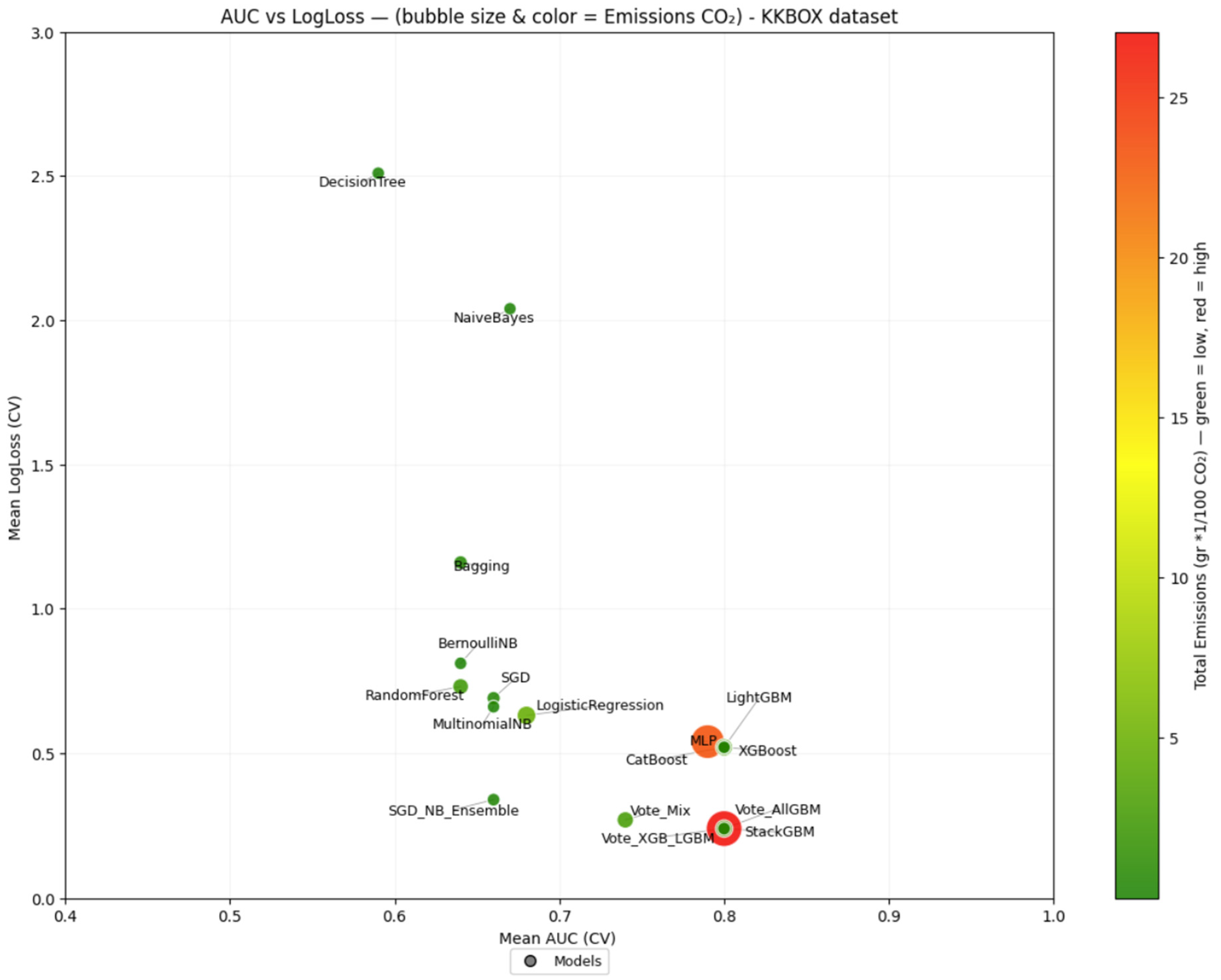
Figure 21 contains the Mean AUC in the x-axis and the Mean Log Loss in the y-axis for 10-fold CV when running on a PC on the KKBOX dataset. Each ML model is represented with a circle. A third parameter, the total emissions (g CO₂) in the same settings (10-fold CV, PC), were added by changing the color and size of the circles. The ML models that have the best predictive performance fall into the right-bottom side of the figure since the AUC is higher and Log Loss is lower. When a circle is small and green, it means that the ML model generated small amounts of emissions. When a circle is larger and redder (color scale from green to red), it generates higher emissions.

For example, Decision Tree, Naïve Bayes and Bagging are worse than MLP and LightGBM since they are positioned more to the left and top. MLP, XGBoost, CatBoost, LightGBM, StackGBM, Vote_AllGBM and Vote_XGB_LGBM noted the best predictive performance since they are on the right and bottom part of the figure. However, MLP and StackGBM circles are bigger than the rest and red, indicating that those models generated higher levels of emissions than the rest of the models. Thus, ML models such as XGBoost, LightGBM, CatBoost and Vote_XGB_LGBM are better to choose than StackGBM and MLP since they have similar predictive performance and are more eco-friendly.

Similarly, for the Telco dataset (Figure 22), the ML models LightGBM, Logistic Regression, CatBoost, Vote_XGB_AllGBM, Vote_XGB_LGBM, XGBoost and StackGBM noted good predictive performance and thus, they are in the bottom right corner of the figure. However, the StackGBM circle is larger and redder, indicating that it generated higher emissions, and it is not an eco-friendly option.

In order to compare the ML models based on multiple objectives such as predictive performance, generated emissions, training time and inference time, we employed the Pareto frontier analysis [58] to identify the ML models that are the best candidate solutions. The aim is to determine which ML models have a high AUC, low Log Loss, low training time and low prediction time. The selected criteria are interrelated; AUC and Log Loss are interrelated since they both calculate predictive performance. Specifically, the AUC shows how well the ML model can separate the two classes of churners and non-churners and Log Loss measures how reliable the predicted probabilities are. Similarly, training time and emissions are interrelated since the longer the training time, the bigger the emissions. Latency could also be considered interrelated with training time, considering that an ML model that takes more time to train, probably needs more time to generate a prediction, since models’ complexity can affect both training time and inference latency.

To this end,

Table 12. Trade-offs between performance–efficiency based on Pareto frontier analysis, on the KKBOX dataset.

Model	Mean AUC	Mean Log Loss	Total Training Time (min)	Total Emissions (g CO2)	Mean Latency (ms)	Pareto Frontier
XGBoost	0.80	0.52	0.34	0.15	1.37 × 10−6	Pareto
LightGBM	0.80	0.52	0.30	0.14	3.71 × 10−6	Pareto
CatBoost	0.80	0.52	6.48	3.09	7.79 × 10−7	Pareto
Logistic Regression	0.68	0.63	11.36	4.76	1.87 × 10−7	Pareto
Decision Tree	0.59	2.51	0.40	0.10	6.67 × 10−7	Pareto
Random Forest	0.64	0.73	8.61	2.23	4.5 × 10−5	Dominated
Naïve Bayes	0.67	2.04	0.10	0.03	1.2 × 10−6	Pareto
MLP	0.79	0.54	78.88	23.21	3.91 × 10−6	Dominated
Vote_XGB_LGBM	0.80	0.24	0.52	0.24	4.94 × 10−6	Pareto
Vote_AllGBM	0.80	0.24	6.58	3.14	5.58 × 10−6	Dominated
Vote_Mix	0.74	0.27	6.70	2.76	3.24 × 10−6	Pareto
StackGBM	0.80	0.24	76.43	27.03	5.24 × 10−5	Dominated
BernoulliNB	0.64	0.81	0.13	0.04	1.72 × 10−6	Dominated
MultinomialNB	0.66	0.66	0.08	0.03	1.07 × 10−6	Pareto
Bagging	0.64	1.16	2.51	0.65	5.97 × 10−6	Dominated
SGD	0.66	0.69	1.87	0.47	1.87 × 10−7	Pareto
SGD_NB_Ensemble	0.66	0.34	0.69	0.18	1.16 × 10−6	Pareto

contains, for each ML model, the mean AUC, mean Log Loss, total training time, total emissions and Mean Latency when ML models run on a PC on the KKBOX dataset. A model is considered a Pareto frontier when it is better than or equal to all objectives and better than at least one. For example, XGBoost is a Pareto frontier because there are no other ML models better on all parameters. On the contrary, VoteAllGBM is dominated by Vote_XGM_LGBM because although they have the same AUC and Log Loss, VoteAllGBM had higher training time, emissions and latency. The last column of Table 12 contains “Pareto” if it is a Pareto frontier and “Dominated” if there are solutions that are better alternatives.

For the Telco dataset, a similar analysis was conducted.

Table 13. Trade-offs between performance–efficiency based on Pareto frontier analysis, on the Telco dataset.

Model	Mean AUC	Mean Log Loss	Total Training Time (min)	Total Emissions (g CO2)	Mean Latency (ms)	Pareto Frontier
XGBoost	0.83	0.50	1.34	0.87	0.000008	Pareto
LightGBM	0.84	0.47	0.91	0.59	0.000005	Pareto
CatBoost	0.84	0.47	13.67	10.02	0.000009	Pareto
Logistic Regression	0.85	0.49	1.27	0.88	0.000001	Pareto
Decision Tree	0.65	9.53	0.36	0.16	0.000002	Pareto
Random Forest	0.83	0.51	4.37	1.88	0.000028	Dominated
Naïve Bayes	0.82	2.88	0.16	0.07	0.000004	Pareto
MLP	0.81	0.55	34.89	18.13	0.000003	Dominated
Vote_XGB_LGBM	0.84	0.44	2.08	1.34	0.000030	Pareto
Vote_AllGBM	0.84	0.43	16.61	12.31	0.000038	Pareto
Vote_Mix	0.83	0.47	2.32	1.56	0.000031	Pareto
StackGBM	0.82	0.50	105.15	73.36	0.000082	Pareto
BernoulliNB	0.81	1.09	0.18	0.09	0.000004	Pareto
MultinomialNB	0.83	0.82	0.15	0.08	0.000002	Pareto
Bagging	0.80	1.31	1.64	0.84	0.000005	Dominated
SGD	0.82	2.69	0.63	0.29	0.000001	Pareto
SGD_NB_Ensemble	0.83	0.84	0.95	0.42	0.000004	Pareto

contains the results, with the last column indicating the Pareto frontier models. For AUC ≥ 0.8 and Log Loss ≤ 0.6, the best candidate solutions are XGBoost, LightGBM, CatBoost, Logistic Regression, Vote_XGB_LGBM, Vote_AllGBM, Vote_Mix and StackGBM.

3.4.2. Green Efficiency Weighted Score (GEWS)

In order to select the best solutions among the best candidates, we defined a Green Efficiency Weighted Score (GEWS). The GEWS is defined as a weighted sum of normalized metrics, the AUC, Log Loss, training time, total emissions and Mean Latency Equation (2), and it is based on the Simple Additive Weighting (SAW) method proposed by MacCrimmon (1968) [59]. The values of the metrics were normalized with the min–max scaling method.

$$GEWS=w_{AUC}\ast AUC+w_L\ast LogLoss+w_T\ast TrainingTime+w_{{co}_2}\ast Emissions+w_{Pr}\ast Latency$$

(2)

The GEWS is considered a useful performance metric for decision makers, as it aims to facilitate SaaS providers towards selecting the most suitable ML model for their needs, based on a set of evaluation metrics, covering (1) predictive performance by considering AUC and Log Loss, (2) efficiency by considering training time and Mean Latency and (3) sustainability by considering CO₂ emissions.

In our case, weights were set as follows: $w_{AUC}$= 0.3, $w_L$= 0.2, $w_T$= 0.15, $w_{{co}_2}$= 0.2 and $w_{Pr}$ = 0.15. In this way, we gave a higher weight to the AUC performance measure, 0.2 for Log Loss, 0.2 for emissions and 0.15 for training and latency. The selection of the weights was defined by our team of computer scientist experts, aiming to represent the case of a typical SaaS provider who is considering predictive performance as a slightly more important metric.

The latter selection of weights is indicative; weights can be adjusted based on the SaaS providers’ preferences. Log Loss is more important for SaaS providers that run expensive campaigns and therefore, are interested in having churn prediction probability scores that can be relied on, while training time is more important for SaaS providers that train churn prediction models frequently. Similarly, latency is more important for SaaS providers that run retention actions based on triggers and use the models in real time, e.g., when a user browses the cancelation page, a personalized discount to appear based on the user’s likelihood of churn. If the latency of the ML model is high, this will impact on the end user experience. For SaaS providers that run predictions in bulk to run retention campaigns, latency may not be that important since it does not affect the end user experience. Finally, emissions may not be of equal importance to all SaaS providers. An SaaS that runs in low-carbon regions generates much less emissions; thus, the emissions measure would be more important for an SaaS that runs on high-carbon regions.

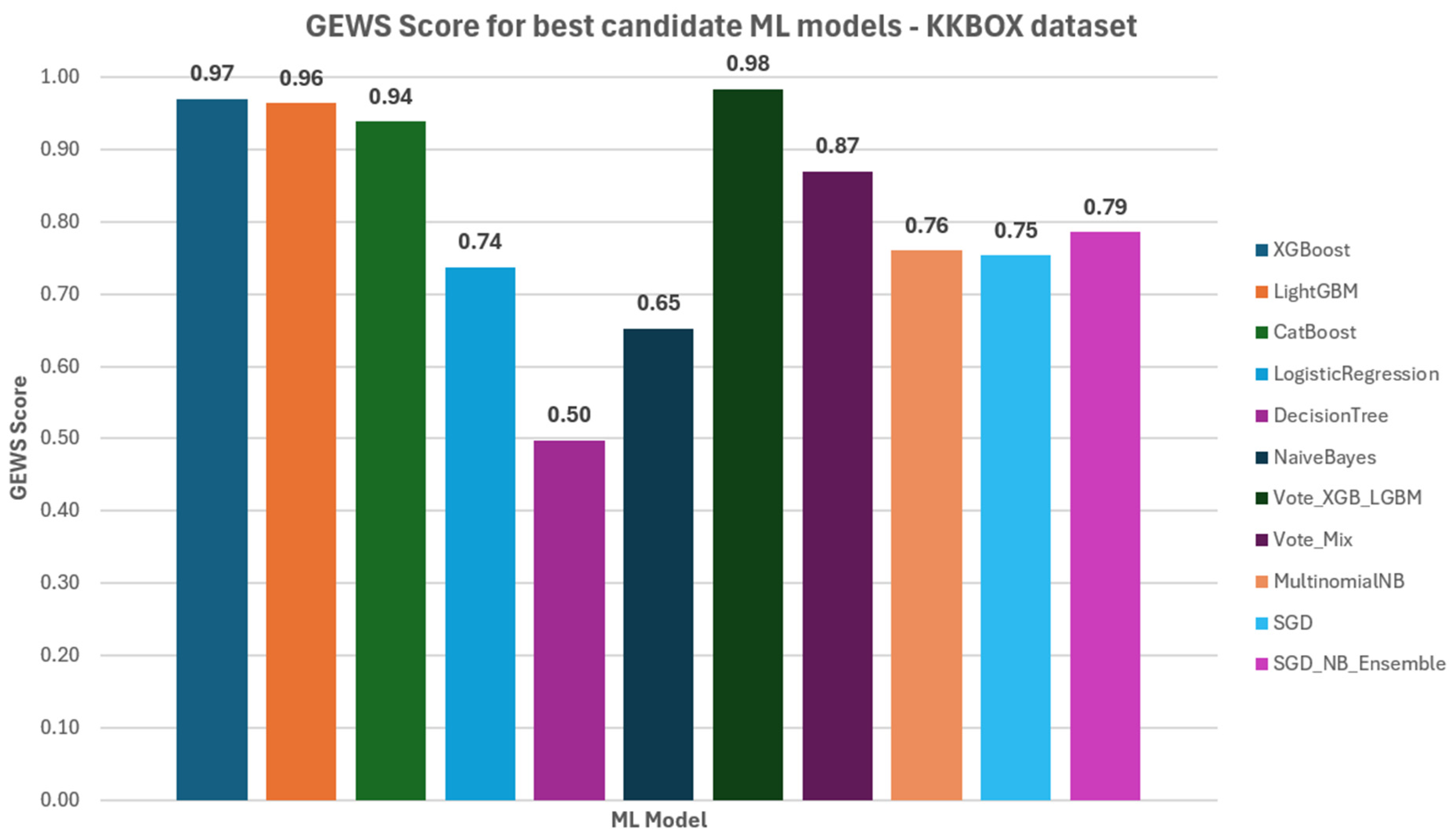
Figure 23 contains the computed GEWSs for the best candidate ML models for the KKBOX dataset on 10-fold CV (as presented in Table 12).

As it is depicted in Figure 23, the best GEWS was achieved by Vote_XGB_LGBM (0.98). The next best scores were noted by XGBoost, which scored 0.97, followed by LightGBM, which scored 0.96. CatBoost had the same AUC and Log Loss with LightGBM but achieved 0.94 GEWS since it had higher training time, emissions and latency. Similarly, Vote_Mix, which noted good AUC and Log Loss measures, but is less eco-friendly and slower than XGBoost and LightGBM, achieved a lower GEWS of 0.87. Finally, ML models that had much lower predictive performance but are fast and generated low emissions achieved scores of 0.79 for Logistic Regression, 0.65 for Naïve Bayes, 0.76 for MultinomialNB and 0.79 for SGD and SGD_NB_Ensemble. Acceptance criteria could also be set in order to exclude solutions that do not meet specific criteria. For example, MultinomialNB, which scored 0.79 because it had a high AUC (0.81), very low values on the training time, prediction time and emissions, but noted a log loss of 0.87, could be excluded from the list of candidates before computing the GEWSs (e.g., acceptance criterion of Log-Loss <0.6).

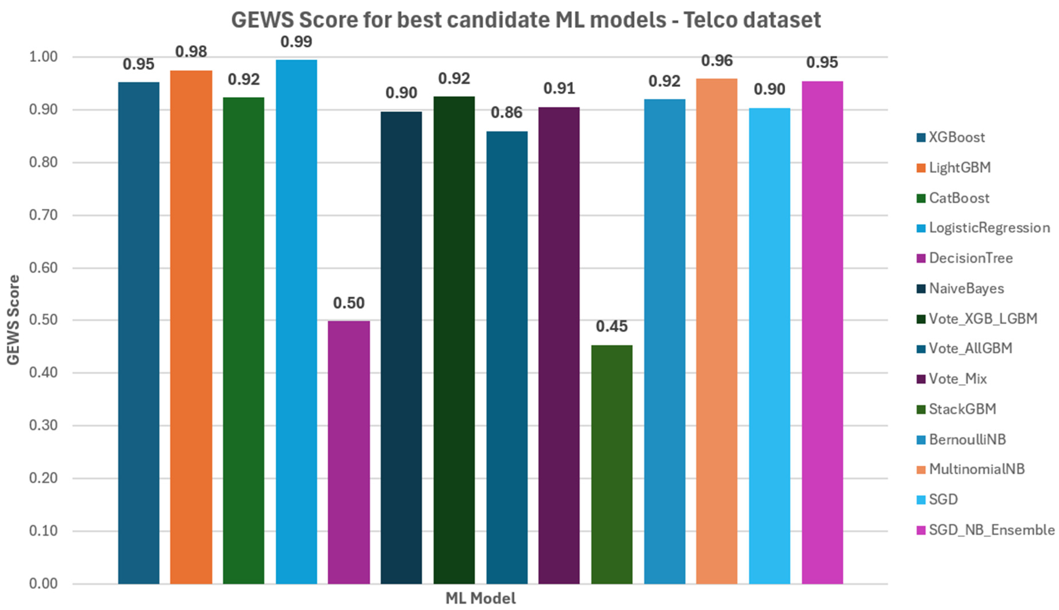
Figure 24 presents the GEWSs for the Telco dataset for the best candidate models. The best GEWS was achieved by Logistic Regression (0.99), followed by LightGBM with 0.98. On the contrary, Vote_XGB_LGBM, which achieved the highest score in the KKBOX dataset, achieved 0.90 on Telco, indicating that simpler alternatives like Logistic Regression are preferable for smaller datasets like Telco. StackGBM, which has a similar AUC and Log Loss (0.82 and 0.5, respectively), achieved a much lower score of 0.45 due to its high training time, emissions and latency. The Bayes models (Naïve Bayes 0.90, BernoulliNB 0.92 and MultinomialNB 0.96) also achieved good scores due to their good AUC and very small training time, emissions and latency. However, if acceptance criteria of Log Loss < 0.6 are set, those ML models do not qualify since they all noted higher values of Log Loss.

4. Discussion

The present work focused on decision support systems for SaaS and, more specifically, for churn prediction, which is of great importance for SaaS providers, on both local and international levels. For regional markets, churn prediction aims to promote business sustainability and resource optimization; churn prediction could help small local businesses to retain their customers through targeted retention strategies and stabilize their revenue, since they often operate on limited budgets and face intense competition. At the international level, churn prediction models can be adapted globally across markets to improve customer retention. Big international firms could benefit from benchmarking to refine their own ML models and lead to innovative retention strategies. Finally, ML models that reduce churn as well as cloud usage are preferable towards contributing to greener AI efforts. To this end, the results of our research are mainly interesting for direct stakeholders that seek actionable insights to reduce churn, like SaaS companies, as well as for data scientists and product managers who use ML models to improve customers’ experience. Moreover, providers of cloud services could also benefit from the presented results, to gain additional insight into efficient deployment and resource usage. Finally, the proposed methodology aims to contribute to the academic sector, and most specifically, to the evolving field of applied ML in the business context. The presented benchmarking should be considered by SaaS developers to refine their churn prediction models, by cloud infrastructure teams to ensure both ML models’ efficiency and sustainability and by researchers interested in sustainability, to evaluate the environmental impact of ML for SaaS in cloud environments.

Most of the related research focused on the accuracy of predictions, neglecting aspects such as training time, inference time, energy consumption and the carbon footprint of the training and deployment of churn-prediction ML models. Therefore, with this work, we benchmarked different ML algorithms in two public datasets and tracked their predictive performance with well-known metrics such as the AUC and more specific ones like Log Loss, which is valuable for SaaS providers that run retention campaigns. Moreover, with our extensive benchmarking process in the cloud, we aimed to determine the relative differences in ML models regarding their carbon footprint and how these change when they run in different regions. Finally, we provided a way to quantify the relative differences and select the best ML models that achieve good trade-offs across the different metrics by introducing a new weighted score, namely the Green Efficiency Weighted Score (GEWS).

The experimentation process revealed that in small datasets, like Telco, simple methods like Logistic Regression can be a good fit, offering a good balance between predictive performance, efficiency and sustainability. In larger datasets like KKBOX, simple ML models like Logistic Regression could not capture the underlying relationships well, showing low AUC and increased energy consumption and carbon footprint, noting the third highest values. On the contrary, XGBoost, LightGBM and the voting schemes of both showed better results. Voting schemes such as Vote_XGB_LGBM and VoteAllGBM were more “conservative” in their predictions, noting low recall values indicating that they missed a lot of churners. However, they noted much lower Log Loss values than the rest of the ML models. Therefore, the probabilities that those ML models generated were more reliable and thus, more suitable for SaaS providers that run expensive campaigns or have limited resources. ML models like XGBoost, LightGBM and CatBoost showed the capability of “catching” more churners; therefore, they seem to be a better alternative for SaaS providers that look to target as many churners as possible.

More complex ensemble approaches like StackingGBM and Vote_Mix did not outperform the simpler voting scheme of XGBoost and LightGBM (Vote_XGB_LGBM) in predictive performance, which noted the same predictive performance metrics (AUC, Log-Loss, accuracy, recall, F-measure and a little higher precision (0.93 vs. 0.91)). The Stacking ensemble (StackGBM) was the most energy-consuming ML model, generating 111 times higher emissions than Vote_XGB_LGBM when run locally. When run on the cloud, StackGBM’s emissions were reported 102 times higher than the emissions of Vote_XGB_LGBM in a high-carbon intensity region (VM1), 101 times higher in a “medium” intensity region (VM2) and 91 times higher in a low-carbon region (VM3). The emissions of training StackGBM in a high-carbon intensity region (VM1) were more than 400 times higher than the emissions when running Vote_XGB_LGBM in a low-carbon region (VM3). Moreover, the training time of StackGBM was 100 times higher than Vote_XGB_LGBM, while the latency was 10 times higher.

Similarly, MLP showed good predictive performance, yet it did not outperform ML methods such as XGBoost and LightGBM, while it showed the second highest training and inference time and higher energy consumption and emissions. The emissions generated were more than five times higher than CatBoost’s emissions, 180 times higher than LightGBM and 100 times higher than the emissions of XGBoost. CatBoost’s training generated 20 times higher emissions than XGBoost and 33 times higher than LightGBM. When MLP was run in a high-carbon intensity region (VM1), it generated 459 times higher emissions than XGBoost, 919 times higher than LightGBM and 25 times higher emissions than CatBoost when run in a low-carbon region (VM3). The experimentation results showed that for the same churn prediction models, the generated emissions can be even up to almost five times higher when running in regions that have higher grid carbon intensity. Therefore, the selection of the region is very crucial for minimizing the carbon footprint of the ML models.

XGBoost, LightGBM, CatBoost and MLP showed to be very fast, noting low latency and high throughput values comparable to the simpler and very fast Bayes models, Decision Tree and SGD. Voting schemes such Vote_XGB_LGBM, Vote_Mix and VoteAllGBM showed higher inference times, which was as expected since they generate the final prediction by more than one ML model. The slowest among the voting schemes was VoteAllGBM, noting 4× Latency than XGBoost, 1.5× latency than LightGBM and 7× latency than CatBoost for the KKBOX dataset and 3.68× latency than XGBoost, 3.27 × latency than LightGBM and 5.89 × latency than CatBoost. Finally, Random Forest and StackGBM showed much higher inference times, indicating that they are not good choices for SaaS providers that use the churn prediction models frequently and have a large user base. For example, StackGMB latency for the KKBOX dataset was 37 times higher than XGBoost, 14 times higher than LightGBM, 65 times higher than CatBoost and 10 times higher than Vote_XGBoost_LGBM. Similarly, for the Telco dataset, StackGBM’s latency was 9.61 times higher than XGBoost, 8.54 times higher than LightGBM and 15.37 times higher than CatBoost.

For selecting the best ML model to use for SaaS churn prediction, we suggested a unified metric, the GEWS, that considers different aspects such as predictive performance, training time, inference time and carbon footprint. This way, SaaS providers can pick the ML model that is more suitable for their case, balancing predictive performance, efficiency and sustainability. Based on the experimentation results, the highest GEWS for the Telco dataset was noted by Logistic Regression, showing that for small datasets, simple models can be sufficient. For the KKBOX dataset, the highest GEWS was achieved by the voting ensemble Vote_XGBoost_LightGBM, offering a good balance of predictive performance, training and inference times along with carbon footprint.

Future work could include experimentation with different hyperparameters for each ML model. Hyperparameters’ optimization could further refine the models’ performance; efficient tuning strategies could be explored to balance performance gains with sustainability concerns. Moreover, the impact of different feature selection, feature engineering and feature transformation approaches could be examined, as well as the use of more deep learning architectures. Different resampling and under-sampling techniques could also be tested, while more state-of-the-art SaaS native datasets could be used.

Most of the ML models in this benchmarking are CPU-based. However, ML models like XGBoost, LightGBM and CatBoost can be trained while using GPU resources. Future work could examine the impact on training time and generated emissions when using GPU compared with CPU training, and how this is consumed by the different computational resources. Parallel computing is also important to explore how it affects the carbon footprint of the SaaS churn prediction models. Finally, future work could also test how training and running the ML models at different times of the day affect the generated emissions.

5. Conclusions

This study performed an extensive benchmark of ML models for SaaS churn prediction, taking into account not only predictive performance metrics but also metrics measuring efficiency of use and environmental impact. To this end, 17 different ML models were trained in two public datasets locally and on the cloud, in three different regions.

Results revealed that for small datasets like Telco, simple models like Logistic Regression can be both fast and eco-friendly. However, when used in larger datasets like KKBOX, Logistic Regression struggled to achieve good predictive performance while consuming increased amounts of energy.

XGBoost and LightGBM shone in both cases, offering a good balance of predictive performance, fast training and inference times and limited emissions. Experimental results confirmed that the selection of a region for running the ML model in the cloud is very crucial for minimizing the carbon footprint of the ML model. The same churn prediction models generated about five times higher emissions when running in a high carbon intensity region compared to when running in a low carbon one. The fastest models were found to be the simplest ones that had weak predictive performance, such as Naïve Bayes, MultinomialNB and SGD.

Most importantly, in this work, a GEWS metric was proposed for ranking ML models based on their predictive performance, training time, inference time and carbon footprint. Consequently, by using the GEWS metric, SaaS providers can easily select ML models that are not only accurate but also efficient and sustainable, achieving good training and inference times while minimizing their carbon footprint.

References

1. Ibrahim, A.M.A.; Abdullah, N.S.; Bahari, M. Software as a Service Challenges: A Systematic Literature Review. In Proceedings of the Future Technologies Conference (FTC) 2022, Vancouver, BC, Canada, 20–21 October 2022; Lecture Notes in Networks and Systems. Springer: Cham, Switzerland, 2023; Volume 3, pp. 257–272, ISBN 9783031183430. [Google Scholar]
2. Gupta, M.; Gupta, D.; Rai, P. Exploring the Impact of Software as a Service (SaaS) on Human Life. EAI Endorsed Trans. Internet Things 2024, 10. [Google Scholar] [CrossRef]
3. Sanches, H.E.; Possebom, A.T.; Aylon, L.B.R. Churn Prediction for SaaS Company with Machine Learning. Innov. Manag. Rev. 2025, 22, 130–142. [Google Scholar] [CrossRef]
4. Phumchusri, N.; Amornvetchayakul, P. Machine Learning Models for Predicting Customer Churn: A Case Study in a Software-as-a-Service Inventory Management Company. Int. J. Bus. Intell. Data Min. 2024, 24, 74–106. [Google Scholar] [CrossRef]
5. Dias, J.R.; Antonio, N. Predicting Customer Churn Using Machine Learning: A Case Study in the Software Industry. J. Mark. Anal. 2025, 13, 111–127. [Google Scholar] [CrossRef]
6. Charizanis, G.; Mavridou, E.; Vrochidou, E.; Kalampokas, T.; Papakostas, G.A. Data-Driven Decision Support in SaaS Cloud-Based Service Models. Appl. Sci. 2025, 15, 6508. [Google Scholar] [CrossRef]
7. Bolón-Canedo, V.; Morán-Fernández, L.; Cancela, B.; Alonso-Betanzos, A. A Review of Green Artificial Intelligence: Towards a More Sustainable Future. Neurocomputing 2024, 599, 128096. [Google Scholar] [CrossRef]
8. Tabbakh, A.; Al Amin, L.; Islam, M.; Mahmud, G.M.I.; Chowdhury, I.K.; Mukta, M.S.H. Towards Sustainable AI: A Comprehensive Framework for Green AI. Discov. Sustain. 2024, 5, 408. [Google Scholar] [CrossRef]
9. Iqbal, M.S.A.; Haroon, M. Sustainable Cloud. In Advances in Science, Engineering and Technology; CRC Press: London, UK, 2025; pp. 457–462. [Google Scholar]
10. The European Parliament and the Council of the European Union Regulation (EU) 2024/1689. Available online: https://eur-lex.europa.eu/legal-content/EN/TXT/HTML/?uri=OJ:L_202401689 (accessed on 5 September 2025).
11. Rahman, M.; Kumar, V. Machine Learning Based Customer Churn Prediction In Banking. In Proceedings of the 2020 4th International Conference on Electronics, Communication and Aerospace Technology (ICECA), Coimbatore, India, 5–7 November 2020; pp. 1196–1201. [Google Scholar]
12. Tékouabou, S.C.K.; Gherghina, Ș.C.; Toulni, H.; Mata, P.N.; Martins, J.M. Towards Explainable Machine Learning for Bank Churn Prediction Using Data Balancing and Ensemble-Based Methods. Mathematics 2022, 10, 2379. [Google Scholar] [CrossRef]
13. de Lima Lemos, R.A.; Silva, T.C.; Tabak, B.M. Propension to Customer Churn in a Financial Institution: A Machine Learning Approach. Neural Comput. Appl. 2022, 34, 11751–11768. [Google Scholar] [CrossRef]
14. AL-Najjar, D.; Al-Rousan, N.; AL-Najjar, H. Machine Learning to Develop Credit Card Customer Churn Prediction. J. Theor. Appl. Electron. Commer. Res. 2022, 17, 1529–1542. [Google Scholar] [CrossRef]
15. Suh, Y. Machine Learning Based Customer Churn Prediction in Home Appliance Rental Business. J. Big Data 2023, 10, 41. [Google Scholar] [CrossRef]
16. Lalwani, P.; Mishra, M.K.; Chadha, J.S.; Sethi, P. Customer Churn Prediction System: A Machine Learning Approach. Computing 2022, 104, 271–294. [Google Scholar] [CrossRef]
17. Rautio, A.J.O. Churn Prediction in SaaS Using Machine Learning. Master’s Thesis, Tampere University, Tampere, Finland, 2019. [Google Scholar]
18. Maan, J.; Maan, H. Customer Churn Prediction Model Using Explainable Machine Learning. arXiv 2023, arXiv:2303.00960. [Google Scholar] [CrossRef]
19. Gregory, B. Predicting Customer Churn: Extreme Gradient Boosting with Temporal Data. arXiv 2018, arXiv:1802.03396. [Google Scholar] [CrossRef]
20. Hu, X.; Zhang, T. Research on User Churn Prediction of Music Platform Based on Integrated Learning. In Proceedings of the 2024 4th International Conference on Artificial Intelligence, Big Data and Algorithms, Zhengzhou, China, 21–23 June 2024; pp. 267–271. [Google Scholar]
21. Nimmagadda, S.; Subramaniam, A.; Wong, M.L. Churn Prediction of Subscription User for a Music Streaming Service; Stanford University: Standford, CA, USA, 2017. [Google Scholar]
22. Gaddam, L. Comparison of Machine Learningalgorithms on Predicting Churn Within Music Streaming Service; Blekinge Institute of Technology: Karlskrona, Sweden, 2022. [Google Scholar]
23. Wu, S.; Yau, W.-C.; Ong, T.-S.; Chong, S.-C. Integrated Churn Prediction and Customer Segmentation Framework for Telco Business. IEEE Access 2021, 9, 62118–62136. [Google Scholar] [CrossRef]
24. Fujo, S.W.; Subramanian, S.; Khder, M.A. Customer Churn Prediction in Telecommunication Industry Using Deep Learning. Inf. Sci. Lett. 2022, 11, 185–198. [Google Scholar] [CrossRef]
25. Saha, S.; Saha, C.; Haque, M.M.; Alam, M.G.R.; Talukder, A. ChurnNet: Deep Learning Enhanced Customer Churn Prediction in Telecommunication Industry. IEEE Access 2024, 12, 4471–4484. [Google Scholar] [CrossRef]
26. Arockia Panimalar, S.; Krishnakumar, A.; Senthil Kumar, S. Intensified Customer Churn Prediction: Connectivity with Weighted Multi-Layer Perceptron and Enhanced Multipath Back Propagation. Expert Syst. Appl. 2025, 265, 125993. [Google Scholar] [CrossRef]
27. Dodge, J.; Prewitt, T.; Tachet des Combes, R.; Odmark, E.; Schwartz, R.; Strubell, E.; Buchanan, W. Measuring the Carbon Intensity of Ai in Cloud Instances. In Proceedings of the 2022 ACM Conference on Fairness, Accountability, and Transparency, Seoul, Republic of Korea, 21–24 June 2022; pp. 1877–1894. [Google Scholar]
28. Sanchez Ramirez, J.; Coussement, K.; De Caigny, A.; Benoit, D.F.; Guliyev, E. Incorporating Usage Data for B2B Churn Prediction Modeling. Ind. Mark. Manag. 2024, 120, 191–205. [Google Scholar] [CrossRef]
29. BlastChar Telco Customer Churn. Available online: https://www.kaggle.com/datasets/blastchar/telco-customer-churn (accessed on 13 September 2025).
30. Geiler, L.; Affeldt, S.; Nadif, M. A Survey on Machine Learning Methods for Churn Prediction. Int. J. Data Sci. Anal. 2022, 14, 217–242. [Google Scholar] [CrossRef]
31. Kolomiiets, A.; Mezentseva, O.; Kolesnikova, K. Customer Churn Prediction in the Software by Subscription Models It Business Using Machine Learning Methods. In Proceedings of the CEUR Workshop Proceedings, Ternopil, Ukraine, 16–18 November 2021. [Google Scholar]
32. Addison, H.; Chiu, A.; McDonald, M.; Kan, W. Yianchen WSDM-KKBox’s Churn Prediction Challenge. Available online: https://www.kaggle.com/competitions/kkbox-churn-prediction-challenge/ (accessed on 12 September 2025).
33. Sckit Learn Compute_Sample_Weight. Available online: https://scikit-learn.org/stable/modules/generated/sklearn.utils.class_weight.compute_sample_weight.html#sklearn.utils.class_weight.compute_sample_weight (accessed on 12 September 2025).
34. Saias, J.; Rato, L.; Gonçalves, T. An Approach to Churn Prediction for Cloud Services Recommendation and User Retention. Information 2022, 13, 227. [Google Scholar] [CrossRef]
35. Rothmeier, K.; Pflanzl, N.; Hullmann, J.A.; Preuss, M. Prediction of Player Churn and Disengagement Based on User Activity Data of a Freemium Online Strategy Game. IEEE Trans. Games 2021, 13, 78–88. [Google Scholar] [CrossRef]
36. ÇALLI, L.; KASIM, S. Using Machine Learning Algorithms to Analyze Customer Churn in the Software as a Service (SaaS) Industry. Acad. Platf. J. Eng. Smart Syst. 2022, 10, 115–123. [Google Scholar] [CrossRef]
37. Ge, Y.; He, S.; Xiong, J.; Brown, D.E. Customer Churn Analysis for a Software-as-a-Service Company. In Proceedings of the 2017 Systems and Information Engineering Design Symposium (SIEDS), Charlottesville, VA, USA, 28 April 2017; pp. 106–111. [Google Scholar]
38. Hoang, H.D.; Cam, N.T. Early Churn Prediction in Freemium Game Mobile Using Transformer-Based Architecture for Tabular Data. In Proceedings of the 2024 IEEE 3rd World Conference on Applied Intelligence and Computing (AIC), Gwalior, India, 27–28 July 2024; pp. 568–573. [Google Scholar]
39. Chakraborty, A.; Raturi, V.; Harsola, S. BBE-LSWCM: A Bootstrapped Ensemble of Long and Short Window Clickstream Models. In Proceedings of the 7th Joint International Conference on Data Science & Management of Data (11th ACM IKDD CODS and 29th COMAD), Bangalore, India, 4–7 January 2024; ACM: New York, NY, USA, 2024; pp. 350–358. [Google Scholar]
40. Gajananan, K.; Loyola, P.; Katsuno, Y.; Munawar, A.; Trent, S.; Satoh, F. Modeling Sentiment Polarity in Support Ticket Data for Predicting Cloud Service Subscription Renewal. In Proceedings of the 2018 IEEE International Conference on Services Computing (SCC), San Francisco, CA, USA, 2–7 July 2018; pp. 49–56. [Google Scholar]
41. Morozov, V.; Mezentseva, O.; Kolomiiets, A.; Proskurin, M. Predicting Customer Churn Using Machine Learning in IT Startups. In Lecture Notes on Data Engineering and Communications Technologies; Springer: Cham, Switzerland, 2022; pp. 645–664. [Google Scholar]
42. Li, R. Bank Customer Churn Prediction Based on Stacking Model. Adv. Econ. Manag. Political Sci. 2025, 185, 42–51. [Google Scholar] [CrossRef]
43. Chen, T.; Guestrin, C. XGBoost: A Scalable Tree Boosting System. In Proceedings of the 22nd ACM SIGKDD International Conference on Knowledge Discovery and Data Mining, San Francisco, CA, USA, 13–17 August 2016; ACM: New York, NY, USA, 2016; pp. 785–794. [Google Scholar]
44. Ke, G.; Meng, Q.; Finley, T.; Wang, T.; Chen, W.; Ma, W.; Ye, Q.; Liu, T.Y. LightGBM: A Highly Efficient Gradient Boosting Decision Tree. In Proceedings of the Advances in Neural Information Processing Systems, Long Beach, CA, USA, 4–9 December 2017; pp. 3149–3157. [Google Scholar]
45. Dorogush, A.V.; Ershov, V.; Gulin, A. CatBoost: Gradient Boosting with Categorical Features Support. arXiv 2018, arXiv:1810.11363. [Google Scholar] [CrossRef]
46. LaValley, M.P. Logistic Regression. Circulation 2008, 117, 2395–2399. [Google Scholar] [CrossRef] [PubMed]
47. Loh, W. Classification and Regression Trees. WIREs Data Min. Knowl. Discov. 2011, 1, 14–23. [Google Scholar] [CrossRef]
48. Breiman, L. Random Forests. Mach. Learn. 2001, 45, 5–32. [Google Scholar] [CrossRef]
49. Frank, E.; Trigg, L.; Holmes, G.; Witten, I.H. Naive Bayes for Regression. Mach. Learn. 2000, 41, 5–25. [Google Scholar] [CrossRef]
50. Glorot, X.; Bengio, Y. Understanding the Difficulty of Training Deep Feedforward Neural Networks. Proc. J. Mach. Learn. Res. 2010, 9, 249–256. [Google Scholar]
51. Wolpert, D.H. Stacked Generalization. Neural Netw. 1992, 5, 241–259. [Google Scholar] [CrossRef]
52. McCallum, A.; Nigam, K. A Comparison of Event Models for Naive Bayes Text Classification. In Proceedings of the AAAI-98 Workshop on Learning for Text Categorization, Madison, WI, USA, 26–27 July 1998; Volume 752, pp. 41–48. [Google Scholar]
53. Manning, C.D.; Raghavan, P.; Schütze, H. Introduction to Information Retrieval; Cambridge University Press: Cambridge, UK, 2008; ISBN 9780521865715. [Google Scholar]
54. Breiman, L. Bagging Predictors. Mach. Learn. 1996, 24, 123–140. [Google Scholar] [CrossRef]
55. Bottou, L. Stochastic Gradient Descent Tricks. In Lecture Notes in Computer Science (Including Subseries Lecture Notes in Artificial Intelligence and Lecture Notes in Bioinformatics); Springer: Berlin/Heidelberg, Germany, 2012; pp. 421–436. ISBN 9783642352881. [Google Scholar]
56. Google. General-Purpose Machine Family for Compute Engine: c4 Machine Series. Available online: https://cloud.google.com/compute/docs/general-purpose-machines#c4_series (accessed on 14 September 2025).
57. Bishop, C.M. Pattern Recognition and Machine Learning (Information Science and Statistics), 1st ed.; Springer: New York, NY, USA, 2006. [Google Scholar]
58. Jahan, A.; Edwards, K.L.; Bahraminasab, M. Multi-Criteria Decision Analysis, 2nd ed.; Elsevier: Amsterdam, The Netherlands, 2013. [Google Scholar]
59. MacCrimmon, K.R. Decision Making Among Multiple–Attribute Alternatives: A Survey and Consolidated Approach; Arpa Order; RAND: Santa Monica, CA, USA, 1968; No. RM4823ARPA. [Google Scholar]
Figure 1. Flow of the proposed methodology.
Futureinternet 17 00467 g001
Figure 2. Average AUC for 10-fold CV, on the KKBOX dataset (PC).
Futureinternet 17 00467 g002
Figure 3. Average Log Loss for 10-fold CV, on the KKBOX dataset (PC).
Futureinternet 17 00467 g003
Figure 4. Average AUC for 10-fold CV, on dataset Telco (PC).
Futureinternet 17 00467 g004
Figure 5. Average Log loss for 10-fold CV, on dataset Telco (PC).
Futureinternet 17 00467 g005
Figure 6. AUC on holdout vs. average AUC for 10-fold CV, on KKBOX dataset (PC).
Futureinternet 17 00467 g006
Figure 7. Log Loss on holdout vs. average Log Loss for 10-fold CV, on KKBOX dataset (PC).
Futureinternet 17 00467 g007
Figure 8. AUC on holdout vs. average AUC for 10-fold CV, on Telco dataset (PC).
Futureinternet 17 00467 g008
Figure 9. Log Loss on holdout vs. average Log Loss for 10-fold CV, on Telco dataset (PC).
Futureinternet 17 00467 g009
Figure 10. Total training time for 10-fold CV, on KKBOX dataset (PC).
Futureinternet 17 00467 g010
Figure 11. Total Training time (seconds) for 10-fold CV, on Telco dataset (PC).
Futureinternet 17 00467 g011
Figure 12. Mean Latency (ms) on VMs (average on regions), on the KKBOX dataset.
Futureinternet 17 00467 g012
Figure 13. Mean Latency (ms) on VMs (average on regions), on the Telco dataset.
Futureinternet 17 00467 g013
Figure 14. Energy consumption of ML models on the KKBOX dataset (PC).
Futureinternet 17 00467 g014
Figure 15. Energy consumption of ML models for the Telco dataset (PC).
Futureinternet 17 00467 g015
Figure 16. Total Emissions of ML models for 10-fold CV on the KKBOX dataset (PC).
Futureinternet 17 00467 g016
Figure 17. Total Emissions of ML models for 10-fold CV on the Telco dataset (PC).
Futureinternet 17 00467 g017
Figure 18. Total emissions for 10-fold CV, on the KKBOX dataset (Google Cloud VMs).
Futureinternet 17 00467 g018
Figure 19. Average model size in VMs (average in regions), on the KKBOX dataset.
Futureinternet 17 00467 g019
Figure 20. Average model size in VMs (average in regions), on the Telco dataset.
Futureinternet 17 00467 g020
Figure 21. AUC vs. Log Loss vs. emissions CO2, on the KKBOX dataset.
Futureinternet 17 00467 g021
Figure 22. AUC vs. Log Loss vs. emissions CO2, on the Telco dataset.
Futureinternet 17 00467 g022
Figure 23. GEWSs for the best candidate ML models for the KKBOX dataset.
Futureinternet 17 00467 g023
Figure 24. GEWSs for the best candidate ML models for the Telco dataset.
Futureinternet 17 00467 g024