1. Introduction
A Digital Twin (DT) is defined as a multiphysics, multiscale, and probabilistic simulation, integrated with a series of complex data that uses the best available physical models, updating information based on sensors, cameras, and other computer elements capable of representing its corresponding twin [
1].
Technological advances in recent decades in various areas, such as the Internet of Things (IoT), Artificial Intelligence, and the cloud, have allowed the digitization of different assets, processes, and systems in the civil engineering sectors, more specifically in road infrastructure. Data models have been introduced for the maintenance and operation of road infrastructures, such as in the maintenance of tunnels, bridges, or pavements [
2].
A key component in developing a DT for road infrastructure is the ability to compute pavement responses, such as deformations, stresses, and deflections, under varying traffic loads and environmental conditions. These structural indicators are essential for predicting pavement performance issues like cracking and rutting.
Real-time data collected from on-site measurements and surveys of vehicles, pavement, and environmental conditions can be used to calculate the stress and strain states within the pavement structure. This information is then integrated into its DT to enable performance prediction. For this, a constant update of the properties of the materials that make up the pavement structure such as wearing course, base, subbase, and subgrade material is necessary [
3].
Since the properties of pavement materials depend on the environment, the relationship between them and environmental parameters must be considered in the DT’s physical model [
4]. In flexible pavements, the asphalt mixture exhibits viscoelastic behavior, meaning its mechanical response is highly sensitive to factors such as temperature, vehicle speed, and load. Tensile deformation in the surface layer can shift from compressive to tensile stress if the bond with the underlying layer deteriorates, which may result from construction flaws or moisture infiltration [
5], therefore, accurate introduction of asphalt mixture conditions is important for simulating pavement responses.
A DT for roads relies on the continuous exchange of data with its environment, including the road itself, which cannot be achieved with traditional infrastructure. To enable this, the physical infrastructure can be equipped with sensors that collect data and transmit it to the DT for storage and further processing [
6].
Several studies have addressed the development of DT for road infrastructure. In [
1], a DT is proposed that acquires and integrates multiple sources of information, including LiDAR samples, environmental conditions, and traffic data. The model also incorporates neural networks (NN) for photogrammetric reconstruction, enabling the monitoring of pavement surface texture and environmental conditions. The NN is trained using high-resolution photographs. Similarly, Ref. [
2] presents a DT framework to support road maintenance, where DT is combined with decision support systems and artificial intelligence (AI) techniques are applied to extract knowledge from data. In [
3], an asphalt pavement modeling software is developed within a DT framework, considering several aspects of vehicle–tire–pavement interaction, such as three-dimensional non-uniform tire contact stress, interface bonding conditions, the viscoelastic behavior of asphalt, and dynamic vehicular loading. Finally, in the work of El Marai et al. [
6], various challenges that DT can help to address are discussed. Their approach employs a fully rotatable camera and Internet of Things devices connected to the DT, which transmit data, including video streams, to both edge and cloud platforms. The recent literature in DT has increasingly focused on data-driven methods for detection. For instance, in the context of DC microgrids, one study [
7] introduced a data-driven framework to detect and localize false data injection attacks. This approach utilizes subspace identification methods to build an input–output model from process data, enabling the design of adaptive residual generators and observers that can identify malicious activity without relying on a precise physical model of the system. Similarly, to address malware threats in resource-constrained embedded systems, another work [
8] developed a data-driven anomaly detection method that uses subcomponent timing information from software execution as its key features. By employing non-intrusive hardware detectors and machine learning classifiers, such as a one-class Support Vector Machine (SVM), this technique effectively identifies sophisticated malware with high accuracy and low false-positive rates, demonstrating the adaptability of data-driven detection to systems with limited computational resources.
Although prior studies have advanced the field, the literature still reveals important gaps. Most approaches continue to depend on high-end and costly sensors such as LiDAR and high-resolution cameras, while the role of AI in leveraging low-cost, widely available sensors remains insufficiently explored. In addition, many works remain at a conceptual level, lacking rigorous mathematical formalization of Digital Twin components and the associated data flows. The mechanisms for efficient transmission and processing of large-scale datasets are also rarely detailed. Finally, there is often no clear framework for translating raw sensor signals into actionable, high-level alerts that can directly support automated and optimized maintenance decisions.
This paper aims to address these gaps by proposing a comprehensive and formalized DT framework for the preventive maintenance of road infrastructure. Our work concentrates on pavement condition assessment through a data-driven methodology that leverages widely accessible sensing technologies. Another contribution is the formalization of the highway’s physical state through a series of state vectors, which quantitatively describe key domains such as structural deformation and surface condition. Furthermore, the proposed conceptual design explicitly outlines a data pipeline architecture that incorporates fog computing nodes for efficient data handling and integrates a rule-based system for generating automated alerts, directly linking sensor data to decision support. To demonstrate this framework, and the use of AI to enhance and extract value from more accessible, low-cost sensor technology, we present a case study that serves as a proof-of-concept for the data-driven modeling component of the proposed DT. The study describe the process of converting raw, vehicle-mounted sensor data into actionable maintenance insights, in this case, pavement surface condition, using a specialized deep learning model as the DT’s analytical engine.
2. Maintenance Systems in Road Infrastructures
The evolution of Pavement Management Systems has been driven by the rapid expansion of road networks and the increasing need for technical, economic, and sustainable decision-making in infrastructure maintenance [
9]. Today, the application of DT technology in road infrastructure it is transforming maintenance practices by enabling predictive, data-driven decision-making [
2]. A DT is a dynamic virtual model of a physical asset, continuously updated with real-time data. In the case of roadways, it integrates sensor inputs and environmental data to simulate current conditions, forecasts deterioration, and plans optimal interventions [
1,
10]. This approach moves beyond reactive maintenance, offering efficiency, extended life, and alignment with sustainability goals. DTs include the use of IoT sensors, remote sensing, cloud computing, and machine learning. Sensors embedded in or near pavements collect structural and environmental data, such as strain, temperature, and high-resolution cameras, drones, generate detailed imagery and 3D surface models [
11,
12]. These data streams are processed in cloud-based platforms and analyzed using ML algorithms capable of automatically detecting and classifying surface distress [
13]. This automation replaces traditional manual inspections, increasing accuracy, safety, and monitoring frequency across large networks. The integration of Building Information Modeling (BIM), big data analytics, and AI allows for holistic asset management throughout the pavement life cycle. DTs now support real-time tracking, life-cycle cost analysis, and sustainability assessments, including energy use and environmental impact of interventions [
14]. As these technologies mature, DTs are becoming new tools for consideration in infrastructure strategies, enhancing resilience, optimizing maintenance, and contributing to the development of intelligent transportation systems.
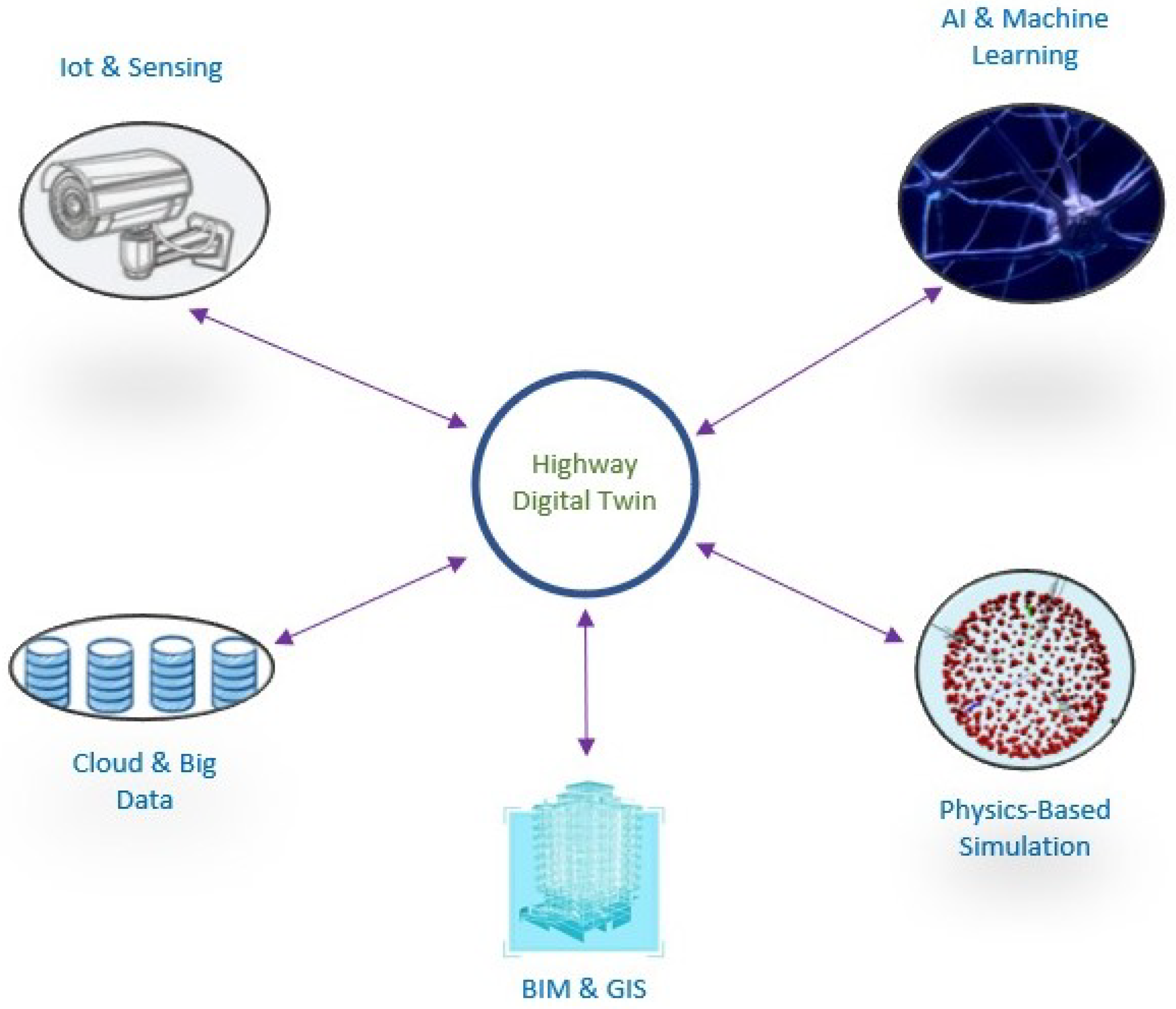
The evolution of DTs in road infrastructure is rooted in several precursor technologies, see
Figure 1, notably Structural Health Monitoring systems, initially developed for bridges and large-scale civil structures [
15]. Another key enabler has been the advancement of BIM, which introduced digital representations of infrastructure assets [
16]. BIM allows data standardization, object classification, and lifecycle documentation, which has influenced the transition from static models to dynamic, real-time DTs [
17].
Although traditional approaches such as Pavement Management Systems, mechanistic-empirical models, and Structural Health Monitoring systems have yielded important advances, they typically operate in isolation and lack an integrated, real-time, and predictive perspective. There remains a critical need for a unified framework that combines physical behavior modeling with continuous data streams across the entire life cycle of road infrastructure assets. This study addresses that gap by proposing a DT based framework, emphasizing the use of vehicle-mounted sensors as mobile data acquisition platforms. These systems enable continuous, automated monitoring, significantly reducing reliance on costly and sporadic manual inspections. Additionally, the integration of a validated machine learning model into the DT architecture illustrates a use case of intelligent and resource-efficient asset management.
3. Materials and Methods
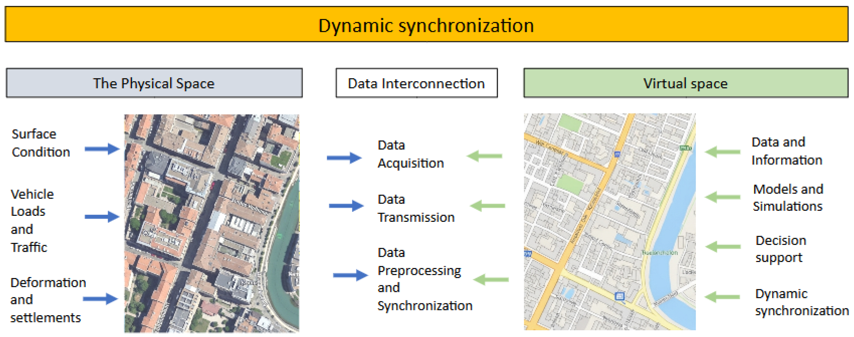
The framework of DT-based for highway infrastructure consists of three parts, involving the physical space, data interconnection, and virtual space, see
Figure 2.
In the physical space, entities involve the highway and the IoT sensors. The IoT devices sense the conditions of the pavement and its surrounding, data from the sensors are collected and transmitted to the virtual space. In addition, IoT devices could execute in real time or not, according to the decision feedback from the DT.
The virtual space consists of four parts, involving data and information module, models and simulations, a decision support module, and a dynamic synchronization process. Each of these components of the proposed DT is described and formalized below. The section is organized into three main subsections.
Section 3.1 describes the Physical Space,
Section 3.2 focuses on the Data Interconnection, and
Section 3.3 introduces the Virtual Space.
3.1. The Physical Space
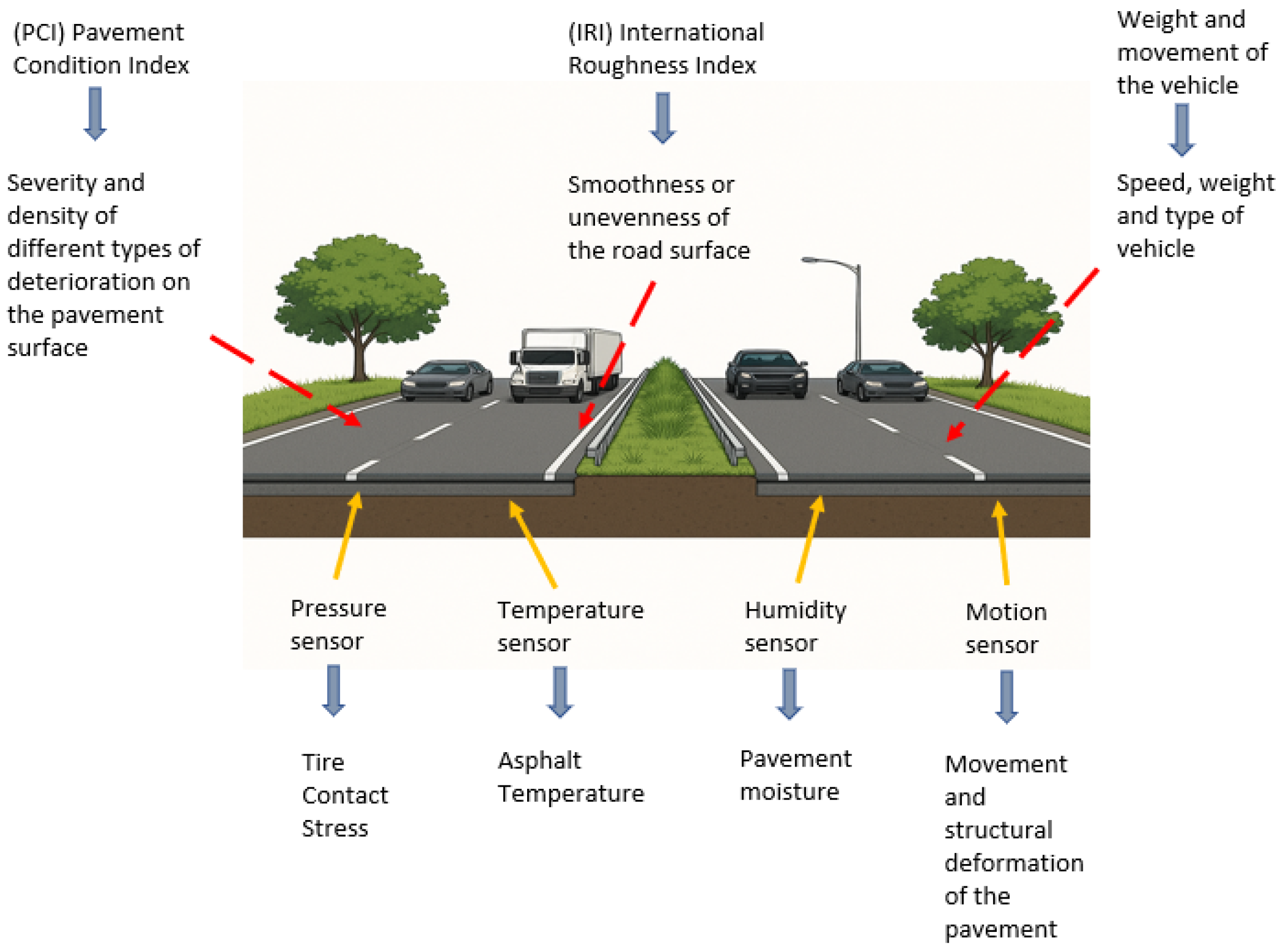
The physical object is the main source for data acquisition, with the highway itself serving as the origin of the data. In the case of the proposed DT, the physical space of interest consists of the highway or road to be monitored. It is worth noting that this physical object cannot be observed, completely, with the naked eye; it is perceived indirectly and partially. A common human observer, when looking at the road, can only perceive the asphalt and the traffic, but cannot quantitatively determine the vehicular load, internal temperature, structural deformations, or subgrade moisture, see
Figure 3.
The purpose of the DT is to provide the observer with an expanded level of detail of the physical object, beyond what is commonly evident. The fidelity of the DT, how closely it represents the physical world, can be quantified by the level of detail of its model and the accuracy of the transferred data.
For the DT to be an effective management and maintenance tool, it must be capable of measuring and modeling the parameters of the physical space that indicate its health status and help detect deterioration early. We are interested in the following monitoring domains and how they are addressed by using modern techniques such as machine learning, in order to be included in the proposal for the DT.
3.1.1. Surface Condition
This domain evaluates the state of the wearing course, which affects safety and comfort. The state is represented by the vector
Selected parameters are Crack Classification (CC) a categorical variable where we adopt the classification from [
18,
19], which categorizes cracks into Block, Longitudinal, Transverse, and Alligator types; the Pavement Condition Index (PCI) [
20], a standard numerical score (0–100) indicating overall surface health; the International Roughness Index (IRI) [
21], which is an indicator used worldwide as a measure of road roughness and correlated with ride quality [
22]; and the Friction Coefficient (
), which indicates the skid resistance of a pavement and has long been acknowledged as a key factor in minimizing traffic accidents, particularly under wet road conditions [
23]. Machine learning has been considered to determine road surface condition classification in [
24] and prediction of PCI in [
25].
3.1.2. Vehicle Loads and Traffic
This domain focuses on quantifying the primary sources of pavement deterioration. The main parameters monitored include Traffic Flow, which involves counting and classifying vehicles. A modern sensing approach for this is the use of video, as demonstrated in [
26]. Another key parameter is the Equivalent Single Axle Loads (ESALs), which converts various vehicle types into an equivalent standard axle load to estimate accumulated traffic damage. The concept of ESAL was introduced by the American Association of State Highway Officials (AASHO) [
27]. In [
28], artificial intelligence techniques have been applied to estimate ESAL values. Additional parameters include vibrations
, representing acceleration signals from structures. These signals can be analyzed in the frequency domain using the Fourier Transform,
, to detect potential structural damage [
29].
3.1.3. Deformations and Settlements
This domain tracks geometric changes in the pavement structure, represented by the state vector
The components include Rutting (
), the depth of longitudinal wheel path depressions; Settlement (
), the vertical displacement of the pavement surface; Strain (
), the material’s stretching or compression under load, defined as
; and Displacement (
), the 3D movement of a pavement section from its original position. Several works in the literature have addressed tracking of these parameters; for example, in [
30] monitoring of road pavement deformations from UAV images is proposed, and in [
31] a prediction of structural numbers in flexible pavements using machine learning is suggested.
The resulting state vectors and models provide a quantitative snapshot of the highway’s condition at any given moment. This multi-domain characterization serves to feed the virtual representation of the twin. The next step consists of defining the data interconnection framework responsible for transferring this information from the physical world to the digital model.
3.2. Data Interconnection
This component acts as the bridge between the physical and virtual domains. Data interconnection enables bidirectional, real-time communication between the physical highway and its virtual representation. Without a robust, accurate, and timely data flow, the DT would become static and obsolete. This layer functions as the nervous system of the DT, here we define three components: data acquisition, data transmission, and data processing for synchronization with the virtual model.
3.2.1. Data Acquisition
This component corresponds to the sensor layer, where physical phenomena are converted into digital signals. As previously discussed in
Section 3.1, each parameter of interest requires a specific sensor type. For highways, the set of sensors, denoted by
, can be expressed as
These sensors are categorized into static and mobile. Static sensors are permanently embedded in the infrastructure and include strain gauges (measuring strain, ), Weigh-In-Motion (WIM) stations (for axle loads, ), inductive loops (for vehicle flow, Q), bridge accelerometers (for vibrations, ), and pavement temperature and moisture sensors (, ). Mobile sensors, on the other hand, are mounted on inspection vehicles and include laser profilometers for measuring the IRI and high-resolution cameras for crack detection and PCI estimation. These sensors typically generate georeferenced outputs, such as tuples .
Each sensor produces a time-dependent signal , resulting in a collection of heterogeneous, asynchronous, and unprocessed data streams.
3.2.2. Data Transmission
After acquisition, data must be transmitted from its location on the highway to a central server or cloud platform for processing. The selected communication technology depends on the sensor’s power requirements, bandwidth needs, and deployment location. High-bandwidth applications, such as video feeds and laser profiling data, may rely on fiber optics or cellular (4G/5G) infrastructure deployed along the highway. In contrast, static sensors with lower data rates may use low power wide area networks such as LoRaWAN, Bluetooth, and SPI.
Additionally, the proposed conceptual design incorporates the use of Fog Computing, which places intermediate fog nodes between the sensors and the cloud. These nodes are responsible for processing and fusing the data locally before transmitting it to the cloud. This approach helps reduce data transmission loads and minimizes latency, as significantly less data needs to be sent over the network. It is assumed that fog nodes are located much closer to the data sources (i.e., the sensors) than the centralized cloud servers.
For instance, in a traffic monitoring application, instead of transmitting raw video streams of a highway to the cloud, which would require substantial bandwidth, the fog node can perform real-time video processing locally and send only the extracted information, such as vehicle positions and classification parameters, to the cloud.
This processed information can be represented as a parameter vector:
where:
: the spatial coordinates of the vehicle,
: the velocity components along the x and y directions,
: an attribute representing the type or load of the vehicle.
This vector encapsulates the essential features required to characterize traffic conditions. Since it is considerably smaller in size compared to raw video data, it results in a substantial reduction in bandwidth consumption during transmission to the cloud, where the DT resides.
This scenario is illustrated in
Figure 4, where the video signal is sent to a fog node located near the camera. In this case, the fog node consists of three modules: two preprocessing modules, denoising and fusion; and a processing module. The denoising module applies a denoising algorithm to each frame of the input video. For optical cameras, the most common noise type is Gaussian noise, although other types of noise may also occur. Several algorithms exist for image denoising that are computationally efficient; one of the most celebrated is the Block-Matching and 3D Filtering (BM3D) algorithm [
32], which has a low computational cost and is suitable for most applications. The next module integrates the output of several algorithms through medium-level fusion [
33], using features obtained by algorithms based on optical flow to determine position and velocity from video [
26,
34]. Finally, the processing module tracks the state vector of each detected vehicle and transmits it to the cloud.
3.2.3. Data Preprocessing and Synchronization
This component preprocesses the input data, because the raw sensor data may be noisy, incomplete, or misaligned in time. Therefore, several operations must be performed before integration.
Noise filtering is the first step. For example, a moving average filter applied to a signal
produces a smoothed version
, computed as
For more dynamic or uncertain systems, filters like the Kalman Filter are used, other specialized denoisers target specific noise types, including Poisson, multiplicative, and salt-and-pepper noise.
Next is data aggregation and fusion. Aggregation refers to computing summary statistics from multiple sensors of the same type. For example, the average temperature across
M sensors in a road section is
Fusion combines data from different sensor types to infer properties not directly measurable. For instance, axle load data () can be fused with strain data () to estimate pavement elasticity.
Finally, synchronization aligns all processed signals to a unified timeline to construct the DT’s state vector:
Each element is a validated and time-aligned parameter. For example, might represent the average IRI at kilometer 5, the vehicle flow Q on a bridge, the maximum strain in a test section, and a categorical surface condition (e.g., dry, wet, icy).
This vector, , constitutes the final output of the interconnection layer. Its structure and accuracy directly determine the reliability and value of the highway’s DT.
3.3. Virtual Space
The virtual object, also referred to as the virtual entity, is the digital representation of its physical counterpart its DT. In the context of a highway DT, it serves as the central block for data integration, analysis, and simulation. It consists of the following components.
3.3.1. Data and Information
This component functions as the primary repository for all data acquired from the physical highway and its surrounding environment throughout its lifecycle. In the context of a highway DT, this repository consists of a highly diverse and large-scale dataset. The total data repository, denoted as
, can be conceptualized as a collection of distinct data types:
The first component, , corresponds to operational and behavioral data, which includes real-time or near-real-time information captured from the highway. This set, referred to as the state vector, comprises structured, semi-structured, and unstructured data. Structured data typically involves time-series readings from sensors, such as strain and temperature , as well as historical traffic tables expressed in terms of Equivalent Single Axle Loads (ESALs), and lists of material properties. Semi-structured data includes formats like JSON or XML derived from external sources such as weather APIs, or graph-based representations of traffic flow. Meanwhile, unstructured data consists of images and video feeds from inspection cameras used for crack detection, audio signals from noise monitoring devices, and raw point cloud data obtained from LiDAR scans.
The second component, , contains the design and specification data that define the original engineering information of the highway. This includes 2D and 3D models, such as CAD drawings of structural elements like bridges and culverts, GIS layers that define the road alignment, and BIM, which integrate both geometric and semantic data. Additionally, this component could make use of specification documents, such as pavement design reports, e.g., asphalt mix designs, specified concrete compressive strength and bills of materials for construction and structural components.
The third component, , refers to historical maintenance data, which provides the DT with the necessary context to learn from past interventions. This includes comprehensive records of maintenance actions—such as the dates and locations of patching, crack sealing, or overlays—as well as historical traffic volumes and documented impacts of extreme weather events. These data allow the DT to incorporate temporal dynamics and inform more accurate predictions and decision-making processes.
3.3.2. Models and Simulations
This is the DT analytical engine module, equipped with a suite of computational models that enable data processing, behavior simulation, and future state prediction. One category of these models is the physics-based approach, which relies on established physical laws and is primarily used for structural analysis.
In this work, we examine traffic simulation, which can be formally characterized by the tuple
as defined by [
35]. The map
M consists of two components: the static semantic map
, which represents drivable areas such as lanes and intersections, and the dynamic environment
, which includes elements such as traffic signals. The dynamic state of the
N actors at time
t is denoted as
, while the collection of decisions at time
t is denoted as
. Each decision
is chosen from a decision space
, decisions could be “go”, “turn”, and “brake”. The objective of traffic simulation is to predict the future actions of all controllable actors given the environment information and the sequence of historical states,
H, through a behavioral model parameterized by
[
35]:
where
f is the model that outputs the future actions for each actor
at time
t and
.
In addition to physics-based models, the DT incorporates data-driven models that learn patterns directly from historical and operational datasets. These are particularly useful for representing phenomena that are too complex to model analytically. For instance, deterioration models employ machine learning algorithms—such as Gradient Boosting or Neural Networks—to predict future pavement conditions.
Moreover, image recognition models based on Convolutional Neural Networks (CNNs) are trained on inspection images to automatically detect and classify pavement cracks. These outputs could be used to compute key condition metrics like the PCI. As a concrete example, a Gated Recurrent Unit (GRU) layers based neural network is presented in
Section 4 as a case study for evaluating pavement surface smoothness and detecting irregularities. The input data for this network originates from recordings obtained during vehicle traversal over the road infrastructure. Specifically, the measurements are captured using an Inertial Measurement Unit (IMU) mounted on the vehicle. The IMU provides time-synchronized multiaxial signals, including linear accelerations and angular velocities along the three spatial axes (x, y, z). It is expected that the sensor readings reflect the dynamic response of the vehicle to pavement surface irregularities. As the vehicle moves, variations in road smoothness—such as bumps, depressions, or potholes—induce characteristic patterns in the IMU signals. By capturing these temporal patterns, the model can learn to distinguish between normal and degraded pavement conditions. The formulation of this model is as follows. We define the input sequence
as a multivariate time series composed of six sensor signals: three-axis accelerometer data and three-axis gyroscope data. Formally, each time step
t contains the following vector:
This time series is used as input to a deep learning model that we designed to classify pavement surface conditions into two categories: normal and depression.
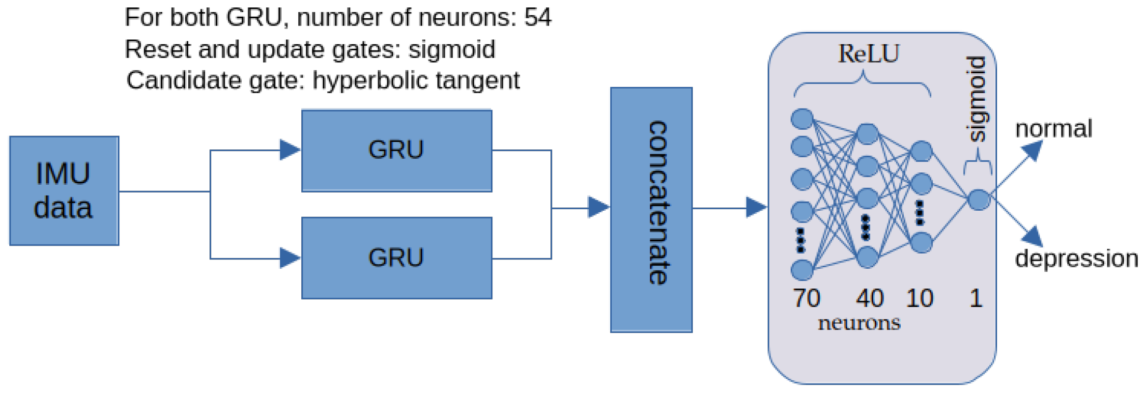
The model architecture consists of two parallel GRU, each processing the full input sequence independently. The output tensors of both GRU layers are then concatenated along the feature dimension and passed through a fully connected (dense) neural network that performs the final classification. This process can be expressed as
Here,
and
denote the outputs of the two parallel GRU layers, ⊕ represents the concatenation operator along the feature axis, and
is a dense neural network responsible for mapping the combined GRU features to a binary classification output indicating pavement condition. This architecture is designed to enhance the model’s capacity to capture diverse temporal patterns from the sensor data by allowing each GRU branch to focus on different aspects of the time series.
Figure 5 shows the network architecture in detail.
Finally, the DT employs 3D and 4D visualization models, integrating geospatial data from systems like GIS and BIM with real-time sensor readings. This integration facilitates an interactive, four-dimensional representation (three spatial dimensions plus time) of the highway’s evolving condition, enhancing decision-making and communication among stakeholders.
3.3.3. Decision Support
The virtual object needs to provide a set of capabilities for highway asset management. This refers to using the prediction and simulation for decision support, for example, through alerts. Prediction enables forecasting the evolution of key performance indicators over time. For instance, it allows predicting degradation curve of the Pavement Condition Index [
36].
Another key feature is the simulation of scenarios, which allows testing the impact of different decisions before their implementation. The system also supports predictive maintenance and anomaly detection, facilitating a shift from reactive to proactive maintenance strategies. Automated alerts can be generated based on predefined rules. One such rule can be formalized as
were
is a predicted parameter at time
t and
is its maximum o minimum safe limit, and common parameters could include the IRI index or the visibility affected by weather conditions.
3.3.4. Dynamic Synchronization
The virtual object is not a static representation; rather, it co-evolves with its physical counterpart through a continuous process of model calibration and data assimilation, commonly referred to as twinning.
This dynamic synchronization is accomplished by constantly updating the virtual object using the state vector , which is retrieved from the interconnection layer. As new data streams in, the state of the virtual object is adjusted to reflect the most current condition of the physical system.
An essential aspect of this process is model calibration. Since predictive models are inherently approximate, they must be recalibrated periodically to maintain accuracy. Calibration ensures that the DT maintains a high level of fidelity over time by aligning the model’s output with empirical observations. This process can be formulated as an optimization problem, where the objective is to determine the set of model parameters, denoted by a vector
. These could be the pavement temperature or traffic for example, and we aim to minimize the discrepancy between the model status or the model predicted responses and the actual sensor measurements. Mathematically, this can be expressed as
Here, represents the model predicted parameters, and is the corresponding measured parameters by sensors from physical object. This continuous feedback loop is necessary to maintaining the alignment between the virtual and physical object across the road’s lifecycle.
4. Results
To validate the practical application of the data-driven models outlined in the Virtual Space
Section 3.3, this section presents a case study focused on road anomaly detection. This experiment is designed to serve as a proof-of-concept, demonstrating how the DT framework can transform low-cost sensor data (from a vehicle’s IMU) into a high-value, automated assessment of pavement condition. The following results validate the effectiveness of the analytical engine component within our proposed architecture.
For the case study, we employed the dataset introduced in [
37], which was designed to support the detection of road surface anomalies using inertial and visual data. The dataset contains synchronized data from three sources collected during urban driving routes: IMU sensors, which record accelerations and rotations; GPS, which provides geographic positioning; and camera images, which capture the visual context simultaneously.
The dataset is stored in pickle (.pkl) files and includes synchronized IMU measurements; accelerometer in m/s2 and gyroscope in rad/s across x, y, z axes. Synchronized GPS information: longitude, latitude, speed, track, and timestamps. Camera data: JPEG images with associated timing. Optionally, annotation labels are provided to indicate anomalies such as manholes, depressions, bumps, and cracks, along with transversity and severity levels (small, medium, high).
The dataset corresponds to a driving session recorded in the city of Larisa, Greece. All three data streams are time-synchronized, so each sample contains IMU readings, GPS coordinates, and the corresponding camera image aligned in time. For a comprehensive description of the dataset, refer to [
37].
In our study, we focused solely on the IMU data, which consists of linear accelerations and angular velocities along three axes (x, y, z). The IMU signals were sampled at 100 Hz. The sensor orientation was calibrated such that the z-axis is perpendicular to the plane defined by the vehicle’s wheels and points upward, the x-axis aligns with the direction of motion, and the y-axis is orthogonal to both x and z.
Each IMU measurement vector is represented as in Equation (
10). To prepare the data for classification, we segmented the IMU recordings into time series windows of 100 samples. Each time window was then labeled according to the majority class among its constituent samples. Using this approach, we extracted a total of 188 time series: 100 labeled as normal road conditions and 88 as road depressions.
To assess the performance of different time series classification approaches, we evaluated a total of six classifiers: Random Forest (RF), Gradient Boosting (GB), AdaBoost (AB), ROCKET from [
38], a recurrent neural network consisting of a Gated Recurrent Unit (GRU) layer followed by a one neuron dense layer, and a custom neural network architecture proposed in Equation (
11), which is composed of two parallel GRU layers.
These classifiers were chosen to represent a diverse set of techniques, including ensemble methods (RF, GB, AB), convolution-based feature extraction ROCKET, and deep learning approaches for sequential data modeling (the GRU-based architecture). The proposed network with parallel GRUs was designed to capture multiple temporal patterns in the input sequence simultaneously, potentially improving the model’s ability to distinguish between subtle class differences in the data.
The dataset was partitioned into training and testing subsets using an 80:20 ratio. That is, 80% of the samples were used for training the models, while the remaining 20% were reserved for evaluating their generalization performance. The models were trained using only the training data and evaluated exclusively on the test set to avoid information leakage and ensure a fair comparison.
Performance was measured using standard classification metrics, including accuracy, precision, recall, F1-score, and Matthews correlation coefficient (MCC) [
39]. These metrics provide complementary insights into the behavior of the classifiers, especially in imbalanced scenarios or when class-specific performance is of interest. The detailed results for each classifier are summarized in
Table 1.
Table 1 summarizes the performance of the evaluated classifiers using six commonly used metrics: accuracy, precision, recall, F1-score, specificity, and MCC.
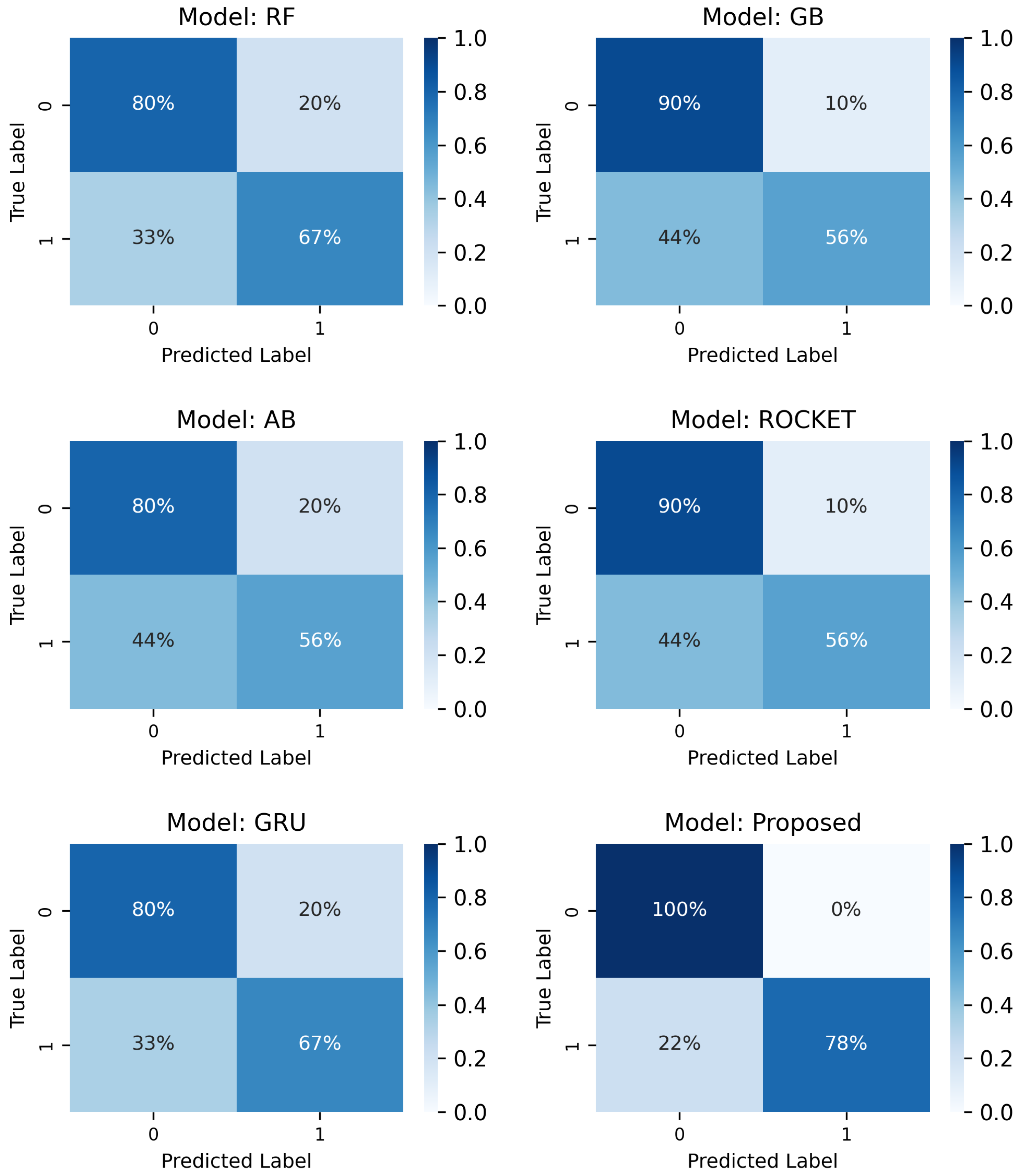
Figure 6 shows the corresponding confusion matrices, and
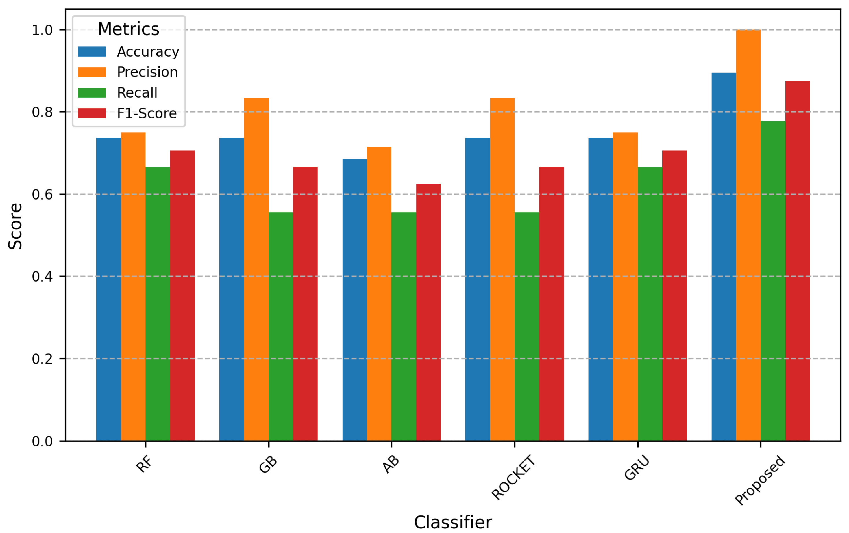
Figure 7 complements the table with a bar chart. These metrics provide evaluation of classification performance, particularly in scenarios where class imbalance or asymmetric costs of misclassification may influence model behavior.
Among the traditional ensemble classifiers, Random Forest (RF), Gradient Boosting (GB), and AdaBoost (AB) yielded similar overall accuracies, ranging from 0.6842 to 0.7368. ROCKET and the GRU-based neural network also achieved accuracies in the same range, with values of 0.7368. Notably, although GB and ROCKET reached high precision values (0.8333), this came at the cost of a lower recall (0.5556), indicating that these models were more conservative and likely biased toward the majority class. This trade-off is also reflected in their moderate F1-scores (0.6667) and MCC values (0.4893).
In contrast, the proposed model—featuring two parallel GRU layers—achieved superior performance across all evaluation metrics. It attained the highest accuracy of 0.8947 and perfect precision of 1.0, meaning it did not produce any false positives on the test set. Additionally, the recall value of 0.7778 suggests the model successfully identified a large proportion of the positive class, with only a small number of false negatives. This balance between precision and recall is reflected in its F1-score of 0.8750, the highest among all classifiers.
Furthermore, the proposed model achieved perfect specificity (1.0), indicating that all negative instances were correctly classified. Its Matthews correlation coefficient (MCC) of 0.8051 significantly outperforms the other models, suggesting a strong correlation between the predicted and true labels, even when considering both classes. This reinforces the robustness and reliability of the proposed architecture for the classification task.
Also, we applied a 5-fold cross-validation procedure to obtain five accuracy values for each classifier. To assess statistical significance, we then performed paired t-tests on the accuracy scores, comparing our proposed method with the baseline classifiers. In all cases, the p-values were below 0.05, confirming that the improvements achieved by the proposed method are statistically significant. The p-values were as follows: Proposed vs. RF: 0.0382, Proposed vs. GB: 0.0388, Proposed vs. AB: 0.0086, Proposed vs. ROCKET: 0.0064, and Proposed vs. GRU: 0.0442.
From these results it can be seen that while conventional ensemble methods and baseline deep learning models provide moderate and similar performance, the proposed parallel GRU network consistently outperforms all others across all metrics. These results highlight the importance of capturing temporal dependencies effectively in time series data and suggest that the architectural choice of parallel recurrent units enhances the model’s capacity to generalize from limited training data.
To provide a more detailed analysis of the parallel GRU model, with respect to the misclassifications for the `pothole’ class (label 1), it can be seen from the confusion matrix of the proposed model,
Figure 6, that 78% of the pothole samples are correctly identified, while 22% are misclassified as normal. Compared to other classifiers, the proposed parallel GRU exhibits a lower false negative rate for potholes, indicating improved sensitivity. This could suggest that most misclassified potholes correspond to extreme or atypical samples, which could represent noisy or highly irregular road conditions. Despite these outliers, the model maintains robust performance, as reflected in the recall of 0.778 and the precision of 1.0.
We now provide an empirical basis for the structural choice of using a parallel GRU architecture. Each GRU is expected to contribute different information to the classification process. Since each GRU has its own independent forget and update gates, this design allows each layer to determine on its own which information to discard and which to retain. Therefore, we expect that the internal states of both GRUs together contain complementary information that can be effectively leveraged by the subsequent dense layer for classification.
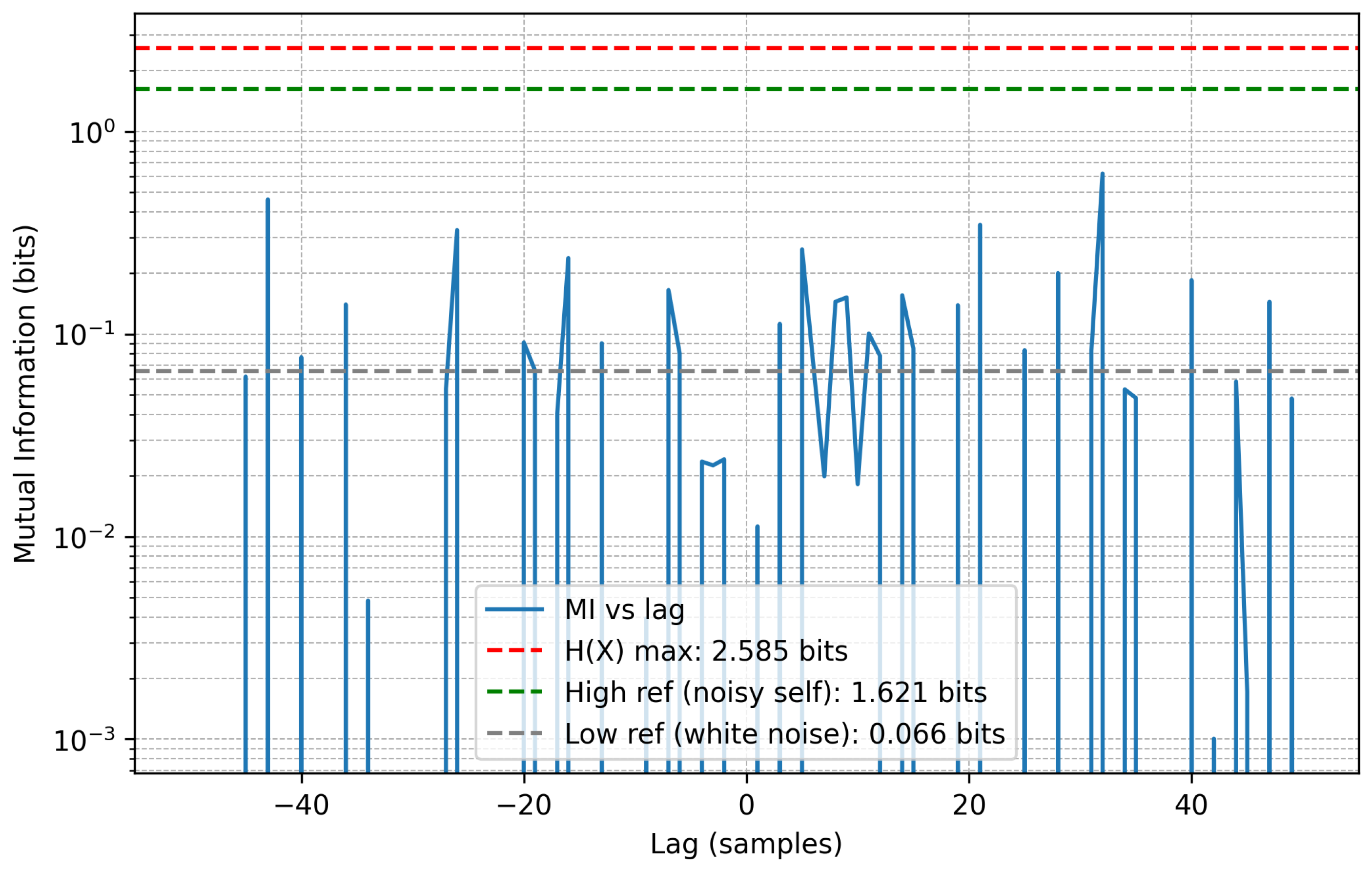
To empirically support this, we computed the mutual information (MI) between the internal states of the two GRUs at different lags, in order to assess whether both states contribute the same information or different information.
Figure 8 shows the empirical MI between the states. The maximum MI occurs at a lag of 32 samples, with a value of 0.620 bits. For reference, the maximum expected MI (the entropy of the state) is 2.585 bits, a high reference obtained from the noisy self is 1.621 bits, and the MI with white noise is 0.066 bits. These results indicate a weak dependency between the GRU states, suggesting that each state contains relevant and non-redundant information.
Finally, it is worth noting that the proposed approach requires parameter calibration; however, this is not pursued further in the present study.
5. Conclusions
This paper presented a formalized framework for a highway DT, detailing the necessary components from physical sensing and data interconnection to virtual simulation and decision support and focusing on pavement condition through surface evaluation. The architecture provides a structured pathway for incorporating a data-driven process for road maintenance. The practical viability of the framework’s data-driven modeling component was demonstrated through a case study on road anomaly detection for assessment of pavement condition. We proposed a parallel-GRU network for anomaly detection, achieving an accuracy of 89.5% and outperforming established classifiers in identifying pavement depressions from low-cost IMU data. This result underscores the potential of using vehicle-mounted sensors as mobile data collection platforms for continuous and automated road monitoring, and could reduce the need for costly and infrequent manual inspections.
The integration of such a validated machine learning model within the broader DT architecture represents a significant step towards intelligent and cost-effective asset management. By enabling real-time condition assessment, authorities can move from scheduled interventions to targeted, on-demand maintenance, thereby enhancing public safety, extending pavement lifecycle, and optimizing the allocation of limited resources. The case of study also shows the fusing old low-cost sensor data with the DT by using the proposed deep learning architecture. The solution in the case study is that the fusion is achieved not by simple data merging, but through a specialized deep learning model, the parallel GRU network, that acts as the fusion engine. The fusion vector being the GRU’s internal states. This model successfully transforms the noisy, high-frequency data from the low-cost IMU sensor into a high-level, actionable insight: the classification of the pavement’s condition.
We acknowledge that the current case study, while successful, focuses on a specific data-driven task. The full potential of the framework will be realized through the integration of this data-driven component with physics-based simulation models and the continuous calibration of the complete twin with real-world data.
Future research will focus on three key areas: (1) expanding the anomaly detection model to classify a wider range of pavement distresses, such as cracks, ruts, and other surface deformations. Many of these anomalies can be detected through an IMU device; this would require expanding the dataset and potentially incorporating more sophisticated layers into the neural network, such as attention mechanisms; (2) implementing physical model calibration using the data pipeline established in our framework. This process will involve fine-tuning key parameters, including the viscoelastic coefficient of asphalt, temperature-dependent material behaviors, and load-response characteristics, to enhance model accuracy and predictive capability; and (3) deploying the end-to-end DT on a physical road segment to validate its performance and utility in a live operational environment.
