User Mobility Modeling in Crowdsourcing Application to Prevent Inference Attacks

Abstract

With the rise of the Internet of Things (IoT), mobile crowdsourcing has become a leading application, leveraging the ubiquitous presence of smartphone users to collect and process data. Spatial crowdsourcing, which assigns tasks based on users’ geographic locations, has proven to be particularly innovative. However, this trend raises significant privacy concerns, particularly regarding the precise geographic data required by these crowdsourcing platforms. Traditional methods, such as dummy locations, spatial cloaking, differential privacy, k-anonymity, and encryption, often fail to mitigate the risks associated with the continuous disclosure of location data. An unauthorized entity could access these data and infer personal information about individuals, such as their home address, workplace, religion, or political affiliations, thus constituting a privacy violation. In this paper, we propose a user mobility model designed to enhance location privacy protection by accurately identifying Points of Interest (POIs) and countering inference attacks. Our main contribution here focuses on user mobility modeling and the introduction of an advanced algorithm for precise POI identification. We evaluate our contributions using GPS data collected from 10 volunteers over a period of 3 months. The results show that our mobility model delivers significant performance and that our POI extraction algorithm outperforms existing approaches.

1. Introduction

The rise of mobile Internet has radically changed the way we access services, ideas, and content. Companies and institutions that once relied exclusively on their employees or specific suppliers to accomplish tasks are now opening up to a wide range of talent worldwide thanks to the magic of crowdsourcing. Jeff Howe first used the term “crowdsourcing” to describe this trend in Wired Magazine in June 2006, highlighting the idea of outsourcing tasks to a large network of people via an open call [1]. In the field of crowdsourcing, one branch stands out: spatial crowdsourcing. This is a practice in which individuals are asked to perform tasks relating to certain places, which frequently involve sharing their physical location. This method can range from the simple transmission of geolocated data, such as real-time traffic reporting or air quality assessment, to more complicated duties that need on-site presence, such as parcel delivery. Uber, for example, uses spatial crowdsourcing to connect drivers and passengers, demonstrating the efficacy of this approach.

However, with the rapid expansion of crowdsourcing, major concerns are emerging about the security and confidentiality of personal data, especially with regard to the location of participants. Crowdsourcing platforms need usually to know the precise geographic location of participants to properly assign tasks, causing a dilemma between the need to share location data and the risks associated with such disclosure. A variety of techniques have been proposed to mitigate the dangers connected with the confidentiality of location data in crowdsourcing. These methods include the use of dummy locations [2,3], spatial cloaking [4], differential privacy [5], k-anonymity [5,6], and encryption [7,8,9]. However, these techniques fail to adequately assess the risk caused by the constant disclosure of participants’ location information to crowdsourcing service providers. Furthermore, a critical but often overlooked feature of location security is vulnerability to inference attacks [10,11], which can infer sensitive information from shared data. Malicious attackers can retrieve sensitive information from location data, even if it is anonymized or masked. Analysis of travel patterns can reveal deeply private personal information, such as individual’s habits, dates, or frequently visited locations, including home and workplace [12]. German politician Malte Spitz used Deutsche Telekom to release six months of his phone’s location data, later publishing it as an interactive map [13]. This case vividly illustrated how combining location data with contextual information could lead to severe privacy breaches. Similarly, a Wall Street Journal report revealed that tech giants like Apple and Google collect vast amounts of location data to develop location-based services, sparking widespread privacy concerns [14]. To safeguard individual privacy, worldwide regulatory initiatives have been launched, including in Europe, the USA, Japan, Australia, and the Asia-Pacific Economic Cooperation. These aim to bolster privacy via bodies like France’s CNIL, proposing standards such as ISO/IEC 29100 for IT security and privacy and AICPA/CICA for personal information risk evaluation [15,16,17,18].

Despite these efforts, regulations alone can’t ensure privacy without data sanitation. Additionally, accurately measuring privacy risks remains a significant challenge. Specifically, when exploring the construction of a user mobility model to bolster privacy protections in crowdsourcing ecosystems, a set of fundamental but challenging issues can be encountered to delve deeper into the realm of data privacy and user behavior:

1.

How can one model user mobility effectively to prevent inference attacks?

2.

How does one accurately pinpoint Points of interest (POIs) to reflect an individual’s movement within a user mobility model?

3.

How does one ensure that the user mobility model remains adaptable to dynamic contexts so as to cope with the flowing nature of user behavior and urban environments?

4.

How does one deal with the challenge of countering inference attacks—what measures to effectively mitigate such threats within crowdsourcing platforms?

These issues form the backbone of our research, guiding us toward developing a nuanced and context-aware framework for privacy protection. In this paper, we primarily focus on the first two challenges and aim to develop a mobility model for implementing inference attacks on crowdsourcing application, with the aim of gaining a deeper understanding of privacy leakage. The mobility model, constructed from the location history of users, provides rich and detailed insight into their movement behaviors. To summarize, our main contributions are as follows:

1.

Offering a comprehensive user mobility graph that provides an unprecedented view of spatial movements and interactions. This contribution is pivotal for designing secured crowdsourcing systems, ensuring that privacy-preserving measures are embedded at the core of digital infrastructures.

2.

Developing an algorithm for the precise identification of POIs, which goes beyond traditional approaches by effectively categorizing significant locations in users’ movement patterns. This enhances not only privacy protection strategies but also provides insights into urban mobility and spatial behavior, potentially influencing urban planning and smart city initiatives.

3.

Evaluating location data disclosure risks via predictive inference attacks that unveil the latent vulnerabilities in existing privacy mechanisms. This critical insight empowers the development of next-generation privacy technologies, making it possible to proactively defend against potential breaches and safeguard sensitive personal information.

The rest of this paper is organized as follows. Section 2 introduces the motivational scenario, discussing the specific challenges our approach aims to address. This clarifies the problems and gaps in current methodologies that our research seeks to fill. Section 3 reviews previous studies on extracting POIs and modeling user mobility. Next, Section 4 describes our proposed approach and the various algorithms we have developed to tackle the identified issues, detailing the theoretical foundation and practical mechanisms of our solution. Section 5 presents the set of experiments conducted to validate our approach, including the experimental methodology, the datasets used, and an analysis of the results obtained. Finally, Section 7 concludes this study by summarizing our main contributions and provides several future directions that we are willing to explore.

2. Motivating Scenario, Challenges, and Objectives

In this section, we explore a real-life scenario to highlight the privacy risks that may arise when a user shares her location with a crowdsourcing platform. Then, we outline our research challenges associated with these risks and describe our dedicated approach.

2.1. Running Example

Let us consider RideEase, an application developed by the company BeeTeam to streamline vehicle sharing among its employees. Environmentally conscious and committed to ecological transition, this initiative offers reward points to encourage the use of sustainable transport solutions, thus motivating employees to adopt eco-friendly carpooling practices. Each year, employees who earn the most points are rewarded. Alice and Bob, two BeeTeam employees, actively use the application to increase their chances of receiving a reward at the end of the year. Bob frequently contributes as a driver, offering rides that coincide with his work schedule and preferred routes. Alice, on the other hand, uses the application to find rides that match her specific needs and schedule. Figure 1 describes how this application works. To effectively recommend routes, Bob must continuously share his location with the application, while Alice only does so when she wants to make a trip. The displayed map (on the right) shows Bob’s usual routes (blue markers) and Alice’s preferred destinations (red markers). The arrows indicate the regular routes taken by Bob, while the dotted lines represent Alice’s potential routes.

However, the use of RideEase raises privacy concerns. For example, if Bob offers rides from his home every morning, this could reveal his home address to regular passengers. Additionally, the history of shared routes could show precise movement patterns, allowing deductions about not only his home but also other frequently visited places (like a gym or a specific supermarket). Similarly, if Alice always chooses routes that drop her off near a clinic she visits regularly, it could inadvertently disclose sensitive information about her private life (such as health details). Repeated use of the application for similar routes might lead other users or even the application’s administrators (who have access to the logs) to notice specific habits, leading to privacy breaches. Assume that Oscar, another employee, secretly exploits RideEase to track his colleagues’ whereabouts, including Bob and Alice, without their consent. By exploiting the system vulnerabilities, Oscar can clandestinely monitor their movements and frequent stops, uncovering many details about their daily routines and compromising their privacy. For example, he could deduce Bob’s precise work hours, his personal activities after work, or Alice’s regular medical visits, thereby severely compromising their security and confidentiality. Here are some examples of the privacy issues that could arise from Oscar’s malicious use of RideEase:

• Blackmail: By discovering sensitive information about their movements, such as visits to health clinics, Oscar could threaten to disclose this information to extort money or other favors from them.
• Stalking or Harassment: Oscar can analyze the frequency and timing of Bob’s and Alice’s visits to certain locations to predict their future movements, allowing for physical stalking or digital harassment.
• Commercial Exploitation: Oscar could sell Bob’s and Alice’s location data to interested companies or individuals, further compromising their privacy and exposing them to unwanted solicitations (e.g., targeted advertising).

However, such semi-reliable nature of RideEase introduces significant privacy concerns.

2.2. Challenges

The primary aim of this research is to construct a user mobility model that facilitates the implementation of inference attacks. This makes it possible to determine what types of sensitive information can be extrapolated from the model, which could potentially compromise an individual’s privacy. The intent is to subsequently use this model to enhance privacy protections for participants in crowdsourcing ecosystems. To develop this nuanced and context-aware framework, one needs to cope with several key scientific challenges, but mainly the following ones that we aim to address here:

1.

Challenge 1: How to understand and analyze user mobility? This challenge requires the consideration of user mobility in order to understand and analyze movements with precision, which safeguards privacy. It involves analyzing data to recognize the regularity of visits to POIs, the paths taken between these points, and the fluctuations in these routines. Advanced data analytics and modeling techniques, such as graphs, are required to encapsulate this complexity in a mobility model. The model must maintain a high degree of accuracy to be effective for inference attacks while implementing robust privacy-preserving measures to protect individual identities.

2.

Challenge 2: How to integrate dynamic contexts? The flowing nature of user behavior and urban environments requires that the user mobility model remains adaptable to dynamic contexts. Taking into account the dynamic context to accommodate different scenarios and environments is essential for it to remain relevant across various user behaviors and conditions. This adaptability involves not only the integration of dynamic and possibly real-time data but also the capacity to adjust to the evolving nature of urban landscapes and user interactions with them. Techniques such as context-aware computing and adaptive algorithms play a pivotal role in ensuring the model’s resilience and relevance.

3.

Challenge 3: How to identify POIs? A pivotal challenge is pinpointing POIs to reflect an individual’s movements within a user mobility model. This necessitates the precise detection and classification of locations that users frequently visit.

3. Related Work

In this section, we establish the foundation by reviewing key studies and methodologies that support our research. First, we examine the strategies for modeling user mobility, as discussed in Section 3.1. Then, we explore the various techniques used for extracting Points of Interest (POIs), as outlined in Section 3.2.

3.1. User Mobility Modeling Techniques

Liu et al. [19] developed an advanced recurrent model called Spatial Temporal Recurrent Neural Networks (ST-RNNs) to improve location prediction accuracy by integrating spatial and temporal contextual information. Utilizing recurrent neural networks, such as LSTM or GRU, this approach is tailored for processing temporal sequences and capturing long-term dependencies, which allow for predictions that are not only accurate but also rich in contextual detail. Traditional methods like the Factorizing Personalized Markov Chain (FPMC) and Tensor Factorization (TF) are limited by independence assumptions and cold start issues. The ST-RNNs model uses time-specific and distance-specific transition matrices to handle continuous time intervals and geographical distances.

In Ref. [20], Li et al. introduced a hybrid model that distinguishes between long-term and short-term preferences using multi-dimensional auxiliary information. The model addresses the limitations of existing methods that often struggle with users having few interactions and overlook the impact of multi-dimensional auxiliary information, such as check-in frequency and POI categories, on user preferences. The proposed model includes a static LSTM module to capture users’ long-term static preferences, a dynamic meta-learning module to capture dynamic preferences, and a POI category filter to comprehensively simulate user preferences.

Gan et al., in [21], employed a hyper-spherical space representation to map user interests utilizing spherical geometry to enhance the accuracy of similarity measurements and the efficiency of clustering algorithms. This innovative approach addresses the limitations of traditional vector spaces by reducing the dimensional curse and improving the interpretability of data points in high-dimensional spaces. This paper explores several case studies where the proposed method has been applied, demonstrating its potential to significantly refine recommendation systems in e-commerce and social networking contexts.

Xu et al. [22] used prediction techniques based on semantic analysis and behavioral data to recommend future visit locations. Employing natural language processing models, they interpreted the semantic context of user activities, which, when combined with machine learning algorithms to analyze behavioral patterns, provides highly personalized and contextually relevant location recommendations. The paper elaborates on the technical challenges and solutions involved in integrating semantic understanding with user behavior modeling, offering insights into the system’s architecture and its application in personalized advertising and urban mobility.

Ganti et al. [23] utilized location traces from taxis to infer human mobility patterns. By employing advanced analytical methods such as trajectory analysis and stochastic process modeling, their study offers valuable insights for urban planning and traffic management. The paper discusses how these data-driven insights can be leveraged to optimize traffic flow and public transportation systems, and it highlights the role of big data analytics in shaping the future of urban mobility.

The comparative analysis presented in

Table 1. Comparison of location modeling techniques.

Criteria
Related Work	Relationships	Spatial and Temporal Dynamics	Scalability and Flexibility	Real-Time Data Handling
Liu et al. [19]	Low	Yes	Medium	No
Li et al. [20]	High	Yes	Medium	Yes
Mingxin et al. [21]	Low	No	Low	No
Xu et al. [22]	High	Yes	High	No
Ganti et al. [23]	Low	Yes	No	Yes
Our Graph-Based Approach
Our Approach	High	Yes	High	Yes

examines several leading user mobility modeling techniques. The evaluation is grounded in four critical criteria: Relationship Modeling, Spatial–Temporal Integration, Scalability, and Real-Time Data Handling. Each criterion assesses a fundamental aspect of the models’ capabilities and performance in real-world scenarios.

• Relationships: This criterion evaluates the model’s ability to depict complex interactions among POIs, which enhances the understanding of user movement patterns and the relevance of contextual data. The evaluation is categorized into three levels. A low level indicates minimal or no depiction of interactions among POIs. A medium level shows some depiction of interactions, but it is not comprehensive. A high level signifies a detailed and comprehensive depiction of complex interactions among POIs.
• Enhanced Spatial and Temporal Dynamics: This criterion focuses on the model’s integration of spatial and temporal data, which is essential for dynamic modeling and providing context-aware recommendations that adapt to real-time environmental changes. The evaluation is binary: either there is no integration of spatial and temporal data, or there is an effective integration of these data types.
• Scalability and Flexibility: This criterion considers the model’s capability to accommodate new data inputs and user preferences efficiently, allowing for updates and customizations without necessitating a complete system overhaul. The evaluation levels are categorized as follows: a low level indicates a limited ability to scale and integrate new data inputs, a medium level denotes a moderate ability to scale and integrate new data inputs, and a high level represents a high capability to scale and integrate new data inputs efficiently.
• Real-Time Data Handling: This criterion examines the model’s effectiveness in processing and integrating data in real-time, which is a critical feature for applications requiring immediate response, such as traffic management and event-driven adaptation strategies. The evaluation is binary: either the model is ineffective in real-time data handling, or it is effective in processing and integrating real-time data.

Table 1 offers an insightful overview of various user mobility models highlighting their diverse capabilities and limitations. Liu et al.’s model [19] excels in spatial–temporal dynamics but face challenges in relationship management and real-time data handling. Li et al.’s modeling [20] has been noted for its effective handling of complex relationships and real-time data, although its scalability is moderate. Mingxin et al.’s work [21] struggles with scalability and real-time responsiveness, though they manage spatial–temporal dynamics to varying degrees. Xu et al.’s work [22] stands out with strong scalability and adept spatial–temporal integration but lacks real-time capabilities.

In contrast, our graph-based model sets a benchmark with high scalability and excellent real-time data handling, effectively adapting to dynamic urban environments without the need for constant recalibration. This model’s integration of advanced graph-based techniques provides precise, contextually-aware insights into urban mobility, leveraging real-time data to enhance traffic management and urban planning significantly. Ganti et al. [23], while their work is capable of real-time data handling, were limited by their model’s lack of scalability, restricting broader application. Our approach, with its comprehensive features, not only matches but surpasses existing models, making it exceptionally suited for sophisticated user mobility solutions.

3.2. Poi Extraction Techniques

The process of pinpointing POIs constitutes a type of inferential attack, leveraging either a heuristic approach or a clustering technique to detect locations that reflect individual’s interests. These POIs could include, for example, someone’s home, workplace, or frequented spots like a gym, cinema, or a political party’s main office. Disclosing an individual’s specific POIs could potentially compromise their privacy, since such data might be exploited to deduce sensitive information.

The vast majority of published work uses threshold-based spatiotemporal clustering methods, where the clusters represent stay segments of the trajectory.

In Ref. [24], the authors introduced an algorithm designed to identify significant places from a series of geographic coordinates. These significant places, characterized by clusters of locations where a user spends a considerable amount of time, are not effectively identified by traditional clustering algorithms. The authors highlight three main limitations of conventional approaches: the need for predefined cluster numbers, the inclusion of irrelevant locations in clusters, and the high computational demand.

The authors of [25] presented a novel approach for evaluating user similarity based on their location histories. The significant contribution of this study is the development of a methodology that leverages spatial and temporal aspects of users’ location data to identify patterns of movement and frequent locations. This method enables the discovery of similarities between users not just based on shared locations but also considering the temporal patterns of their visits.

Löwens et al. in [26] introduced DeepStay, a transformer-based model trained under weak and self-supervision on location trajectories to predict stay regions. This model, the first of its kind in deep learning evaluated on a public, labeled dataset, outperformed existing methods in extracting stay regions. DeepStay also significantly enhancedre the detection of transportation modes from GPS trajectories, demonstrating its utility beyond mere POI extraction.

Zhou et al. introduced in [27] a method for POIs utilizing a spatiotemporal adaptation of DBSCAN, termed DJ cluster. This algorithm adjusts to the specific mobility patterns of the individual being analyzed, differing from k-means where the quantity of clusters must be predetermined. Specifically, the DJ cluster algorithm requires only the maximum radius of clusters and the minimum number of mobility traces within a cluster as input parameters, making it a flexible approach for POI extraction based on individual behavior.

In their study, Khetrapaul et al. [28] analyzed data from 62 Geolife [29] users to identify common POIs by detecting stops—locations where a user remains beyond a set time and distance threshold—merging these stops into POIs based on distance, time, and frequency criteria. Krumm [11] introduced a heuristic based on the likelihood of a user being at home at specific times, suggesting the highest probability occurs from 6PM to 8AM, with a median home location error of 61 m in a study of 172 drivers. Similarly, Scellato et al. [30] extracted POIs through analyzing temporal patterns of arrivals and durations at locations using GPS and WiFi logs, offering insights into movement patterns and significant locations.

Table 2. Comparison of POI extraction approaches.

Criteria
Approaches	Parameter Sensitivity	Noise Sensitivity	Temporal Granularity Dependency	Semantic Consideration
Kang et al. [24,31]	high	medium	no	no
Li et al. [25]	high	medium	yes	no
Löwens et al. [26]	medium	low	no	no
Zhou et al. [27]	high	high	no	no
Khetarpaul et al. [28]	low	medium	no	no
Krumm et al. [11]	low	medium	yes	yes
Scellato et al. [30]	low	high	no	no
Our Approach	low	medium	yes	yes

provides a comparative analysis of various POI extraction approaches based on four key criteria: parameter sensitivity, noise sensitivity, temporal granularity dependency, and semantic consideration.

• Parameter Sensitivity: This criterion evaluates how changes in parameters, such as distance thresholds or the minimum number of points in a cluster, affect the extraction results. The sensitivity levels are categorized as follows: high sensitivity indicates that minor parameter adjustments significantly affect the outcomes, medium sensitivity means that changes in parameters lead to moderate variations in the results, and low sensitivity shows that the results are stable and exhibit little variation despite changes in parameters.
• Noise Sensitivity: This criterion evaluates the method’s robustness in handling noisy data, including outliers or irrelevant data points. Sensitivity levels are defined as follows: high sensitivity means that the presence of noise substantially degrades the accuracy of the extraction, medium sensitivity indicates that noise affects the results but the impact is generally manageable, and low sensitivity shows that the method retains accuracy even with significant levels of noise.
• Temporal Granularity Dependency: This criterion assesses whether the effectiveness of the method is influenced by the temporal resolution of the data. It is analyzed as follows: if the accuracy of POI extraction improves with finer temporal granularity, the answer is yes; if the method delivers consistent performance regardless of the temporal resolution, the answer is no.
• Semantic Consideration: This criterion indicates whether the method utilizes semantic analysis to understand the context or significance of locations. Semantic consideration can be evaluated as follows: if semantic analysis is integral and enhances the contextual relevance of the extracted POIs, the answer is yes; if the method relies solely on geographical and temporal data without incorporating semantic interpretations, the answer is no.

Approaches employing clustering, exemplified by Kang et al. [24,31], Li et al. [25], and others, generally exhibit high parameter sensitivity and moderate noise sensitivity, with minimal dependency on temporal granularity and lacking in semantic consideration. Conversely, heuristic-based methods, as seen with Krumm et al. [11], show varied sensitivity to parameters and noise, but they are distinctive in their occasional integration of semantic analysis.

Our approach distinguishes itself by demonstrating low sensitivity to parameters, enabling stable and robust POI extraction. It uniquely benefits from fine temporal granularity and incorporates comprehensive semantic analysis, which significantly enhances the contextual relevance and accuracy of the extracted POIs. This makes it an advanced solution within the spectrum of existing methodologies, offering substantial improvements in both the precision and utility of POI extraction for user privacy.

4. Proposed Approach

In this section, we present our model designed for mobility analysis and the corresponding algorithm for extracting POIs. The main objective of our approach is to leverage advanced graph-based techniques to dynamically interpret and analyze user movement patterns within urban environments. We aim to provide predictive insights that are not only accurate but also rich in contextual relevance. Here, we describe the model’s architecture, focusing on how we generate the mobility graph and the algorithmic strategies employed for data processing, graph formalism, and POI extraction.

4.1. Contribution Insights

Figure 2 provides an overview of our approach which is able to generate user mobility within the context of crowdsourcing. It contains several phases. The initial phase begins with the collection of raw GPS trajectory data. These data typically consist of sequential location points captured at regular intervals, representing the routes taken by participants. However, raw GPS data often contain a significant level of noise and redundant information due to GPS signal inaccuracies and other environmental factors. Therefore, we apply a preprocessing process on the historical location data in order to clean and organize them in several ways.

In fact, this preprocessing algorithm allows us to reduce noise, extract metadata, eliminate short stays and redundancy, and filter out unimportant locations. This process transforms the raw data into a more usable format for the subsequent stages of analysis. Once the data are preprocessed, the graph generation phase starts. In this phase, as presented in Section 4.4, significant locations are identified and defined as nodes. Then, edges are created to represent the paths between these nodes and annotated with corresponding weights while preserving the temporal sequence of the journeys. The final phase includes the POI extraction algorithm, which is detailed in Section 4.5. This algorithm refines the graph by identifying significant POIs, which are locations of particular interest to the participants. This helps to simplify the graph, highlighting the main movement patterns and key locations. The reduced graph contains actual, detailed information about the user’s movements and locations. While this reduction process focuses on relevant data points, it still maintains significant information that could potentially reveal sensitive details about the user. The nodes and edges in the reduced graph represent real POIs and transitions, which can include personal places such as home, work, or frequently visited locations. As a result, the graph retains the potential to expose private aspects of the user’s life. In our future work, we will implement measures to protect user privacy within the reduced graph, ensuring that sensitive information remains secure.

This approach ensures that the generated graph accurately represents the true movement patterns of users. It enhances the efficiency of the analysis by reducing data complexity and provides deeper insights into user mobility, enabling a better understanding of user movement behaviors.

In the following section, we present several preliminary definitions before detailing each step of our approach.

4.2. Preliminaries

Definition 1. 

Mobility Graph is a structured directed graph that represents the historical location data of a user in crowdsourcing application. Formally, our Mobility Graph G is represented as follows:

$$\begin{array}{c}\hfill G=(\mathcal{V},\mathcal{E},\mathcal{M},\mathcal{W},f_W,f_M)\mathit{where}:\end{array}$$

• $\mathcal{V}=\{v_1,v_2,...,v_n\}$ is a set of vertices. Each vertex $v_i$ represents a significant location defined as a specific location frequently visited by a user and uniquely identified (e.g., UUIDs, system-specific codes, or addresses).
• $\mathcal{E}=\{e_1,e_2,...,e_n\}$ is a set of edges, where each edge $e_i=(s,t)$ represents a relation between two locations, with s (source) and t (target) being vertices in $\mathcal{V}$.
• $\mathcal{M}$ is a set of contextual metadata elements designed to enrich the understanding of $\mathcal{V}$ and $\mathcal{E}$ in a graph. These elements encapsulate a variety of contextual details related to significant locations and their connections, extending insights beyond simple geographical or categorical data. The diversity and richness of $\mathcal{M}$ facilitate sophisticated analyses and interpretations, enabling nuanced interactions and informed decisions. Each metadata value m is represented as a key–value pair as follows:

  $$\begin{array}{c}\hfill m=\langle attribute:value\rangle \end{array}$$

  where

  -

  $attribute$ (string): The key ($attribute$) is a string that denotes the name of the metadata component (such as “name” or “address”).

  -

  $value$: The value ($value$) is the specific information corresponding to the attribute, which can vary in type.

  It is worthy to note that some standard metadata components such as name, address, coordinates, and category play a crucial role in providing a comprehensive and unified understanding of each significant location. They enable efficient data processing, facilitate accurate geolocation, enhance searchability, and support semantic querying across different systems and applications. The following are the standard metadata components along with their descriptions:

  -

  Name (string): The significant location official or commonly used name. Examples include “Eiffel Tower” and “Central Park”.

  -

  Address (string): The physical location of the significant location, including street address, city, state, and country. An example is “5 Avenue Anatole France, 75007 Paris, France”.

  -

  Coordinates (C): Geographical coordinates that delineate the significant locations boundaries. These can form simple shapes or complex polygons, offering a precise geographical footprint (cf. Definition 2).

  -

  Category (string[]): A hierarchical structure describing the category of the significant location (cf. Definition 3).

• $\mathcal{W}$ is a set of numeric values representing weights.
• $f_W:\mathcal{E}\to \mathcal{P}\left(W\right)$ is a weighting function that maps each edge e in the set of edges $\mathcal{E}$ to the following statistics attribute S, offering a detailed characterization of the relationship between two significant locations:

  $$\begin{array}{c}\hfill S=\langle ts,td,fs,st,dt\rangle \end{array}$$

  where

  -

  $ts$ (integer): Denotes the time segment during which the movement occurs, offering a time-bound context to the frequency and duration of trips.

  -

  $td$ (integer): Classifies the movements based on the type of day, such as weekdays, weekends, or holidays, adding a layer of temporal classification to the analysis.

  -

  $fs$ (integer): Denotes the frequency of visits between s and t within a given time frame $ts$, highlighting the regularity or irregularity of these movements.

  -

  $st$ (integer): Represents the duration of the user’s stay at location s before departing to location t at $ts$ and $td$, respectively.

  -

  $dt$ (double): Represents the average duration of travel from s to t, providing a temporal measurement of the movement.

  This enriched representation allows for a nuanced understanding of the edges, offering insights into the temporal patterns, intensity of connections, and spatial dynamics among significant locations.
• $f_M:(\mathcal{V}\cup \mathcal{E})\to \mathcal{P}\left(\mathcal{M}\right)$ is a function that associates each vertex $v\in \mathcal{V}$ or each edge $e\in \mathcal{E}$ with a subset of contextual metadata elements from the power set $\mathcal{P}\left(\mathcal{M}\right)$, which is the set of all subsets of $\mathcal{M}$. This association allows for a highly flexible and comprehensive enrichment of each graph component, whether points of interest or their connections, with a wide range of contextual information.

Definition 2. 

Geographical Coordinate is a tuple that contains latitude and longitude. This can be formally represented as follows:

$$c=\langle \mathit{lat},\mathit{lng}\rangle \mid \mathit{lat}\in \mathbb{R},\mathit{lng}\in \mathbb{R}$$

Example 1. 

Consider a park bounded by the following geographical coordinates marking each of the four corners, thereby forming a trapezoid that outlines the park’s perimeter:

Definition 3. 

Hierarchical Category consists of an ordered list of strings describing the category of the significant location at different levels of granularity. This is formally defined as follows:

$$CA=[c_1,c_2,...,c_n]$$

where

• $c_1$ represents the most general category, indicating the broad classification under which the significant location falls.
• $c_n$ is the most specific detail within the category, providing the finest level of classification detail for the significant location.
• Each $c_i$ (for $1<i\le n$) refines the description provided by its predecessor, thereby offering a more detailed and nuanced classification at each subsequent level.

Example 2. 

Using the North American Industry Classification System (NAICS) as an example, the hierarchical category structure can be illustrated as follows:

$$\begin{array}{c}\hfill CA=[“NAICS:452110”,“Restaurant”,“Italian”]\end{array}$$

where

• NAICS:452110 identifies the entity within the general category of “Full-service restaurants”.
• Restaurant further refines this category to denote the type of establishment.
• Italian adds an additional level of specificity, indicating the specific cuisine offered by the restaurant.

4.3. Data Preprocessing

In crowdsourcing architecture, the worker must continuously share his/her location, allowing the platform to collect raw coordinates (latitude and longitude) and compare them with the requester’s position when assigning tasks. However, when the worker accepts a task posted by a requester, the collected physical address provides a more precise position. We assume here the case where the worker continuously shares his/her location to improve data quality. The data preprocessing phase is essential for the development of our mobility model. It involves cleaning, structuring, and enriching raw location data to facilitate subsequent analysis, POI identification, and modeling. This phase ensures that the data are in a suitable format for further processing, leading to more accurate and meaningful insights.

As shown in Figure 3, several intermediate steps for the preprocessing of user coordinates are adopted:

• Noise reduction: A filtering is applied to the coordinates in order to reduce impulsive noise. This filtering consists of replacing each data point with the median of a set of neighboring points in a sliding window. This makes the data smoother and eliminates outliers without over-smoothing important details. In our study, we apply the Median filtering computed as follows:

  $$\mathrm{filtered}\_\mathrm{coordinate}\left[i\right]=\mathrm{median}\left(\mathrm{window}\left(\mathrm{coordinates}[i-{\displaystyle \frac{w}{2}}:i+{\displaystyle \frac{w}{2}}]\right)\right)$$

  where w is the size of the sliding window. This formula indicates that for each coordinate at position i, the filtered coordinate is obtained by taking the median of the coordinates within the window centered around i.
• Metadata Extraction: For each coordinate, metadata are retrieved using an external API (Google Maps, OpenStreeMap, Salesforce Map, etc.). These metadata provide context to the coordinates, including details such as place names, addresses, categories (e.g., restaurant, park, store), etc.
• Unimportant Location Removal: Not all locations recorded in the raw data are significant for the analysis. This step filters out locations that are deemed unimportant or irrelevant to the study. Predefined criteria are applied to identify and remove locations that do not contribute meaningful information. These criteria could include factors such as visit duration, location type, or frequency of visits. By removing these unimportant locations, the dataset becomes more focused and manageable.
• Check Redundant Data: Duplicate entries can skew the analysis and lead to incorrect conclusions. This step ensures that redundant data points are identified and consolidated. Each location point is compared with the previous ones to detect duplicates. If a location point has the same metadata as a previous entry, it is considered a duplicate and is either merged with the existing entry or removed. This reduces redundancy and ensures that each location is unique in the graph.
• Short Stays Removal: Short stays at locations often represent transient activities that are not significant for mobility modeling. This step filters out such short stays to focus on more meaningful visits. The duration of each stay at a location is examined. If the stay duration falls below a certain threshold, the location is removed from the dataset. This helps in focusing on locations where users spend significant amounts of time, which are more relevant for understanding mobility patterns.

The pseudo-code of our preprocessing is provided in Algorithm 1. To illustrate it,

Table 3. Sample coordinates.

Lat	Lng	Timestamp
48.858370	2.294481	2023-01-01 10:00:00
48.858250	2.294300	2023-01-01 10:01:00
48.858370	2.294481	2023-01-01 10:02:00
—	—	—
—	—	—
48.8567838	2.2253981	2023-01-01 23:57:00
48.8572669	2.2261038	2023-01-01 23:58:00
48.8556536	2.2264949	2023-01-01 23:59:00

provides an example of input coordinates. This table includes a series of coordinates with their respective timestamps, representing raw location data that will be processed by the algorithm. The algorithm performs several key preprocessing steps. First, in line 7, median filtering (ApplyMedianFilter ) is applied to the list of locations L to reduce impulsive noise, ensuring that the data are smoothed without losing important details. Then, in line 8, the RemoveShortStays function is called to eliminate short stays, which are often insignificant for mobility modeling. In each iteration of the ForAll loop (line 9), metadata are retrieved for each location (line 10) using the RetrieveMetadata function, which queries an external API to obtain contextual information such as place names, addresses, and categories. The function RetrieveMetadataAttributeByName retrieves the address of the last location (line 11). Duplication checks are performed in lines 12–15: if the extracted metadata for a coordinate have the same address as the last entry added to the list $\mathcal{P}$, they are ignored to avoid duplicates.

Algorithm 1. PreprocessLocations Algorithm.

1: procedurePreprocessLocations($L,w,timer$)   2:     Input: L           ▹ represent the list of user locations dataset   3:         w                ▹ Size of the sliding window   4:         $timer$              ▹ Time threshold for short stays   5:     Output: $\mathcal{P}$            ▹ Preprocessed list of user locations   6:     $\mathcal{P}\leftarrow \left[\right]$   7:     $L\leftarrow$NoiceReduction(L,w)     ▹ Apply median filter to reduce noise   8:     $L\leftarrow$RemoveShortStays($L,timer$)    ▹ Remove short stays from input list   9:     for all $l\in L$ do 10:         $\mathcal{M}\leftarrow$RetrieveMetadata(l.lat,l.lng)    ▹ Extract metadata 11:         $address\leftarrow$RetrieveMetadataAttributeByName$(\mathcal{M},“\mathrm{address}”)$ 12:         if not $\mathcal{P}$or$address\ne \mathcal{P}[-1].id$then  ▹ Check duplication 13:            if IsImportantLocation($address$) then  ▹ Filter locations 14:                $id\leftarrow address$ 15:                $\mathcal{P}\leftarrow \mathcal{P}\cup id,f_M\left(\{id,\mathcal{M}\}\right),l.timestamp$ ▹ Add location with metadata 16:            end if 17:         end if 18:     end for 19:     return $\mathcal{P}$ 20: end procedure

The IsImportantLocation function (line 13) is used to filter locations based on predefined criteria. If the location is deemed important, it is added to the list M with its timestamp (line 14). Finally, the algorithm returns the list P of processed locations (line 19), providing a relevant and clean dataset ready for further analysis.

Table 4. Example output coordinates.

Address	Timestamp	Category	Coordinates
Av. Gustave Eiffel, 75007 Paris	2023-01-01 10:00:00	historical, landmark	[48.858370, 2.294481, 48.858370, 2.294481]
Hôtel Muguet, 11 Rue Chevert, 75007 Paris	2023-01-01 23:56:00	Accommodation	[48.8572669, 2.2261038, 48.8572669, 2.2261038]

shows the output of Algorithm 1 when applied on the coordinates of Table 3.

In this table, each row represents an important location identified by the algorithm. The Address column shows the address of the location, Timestamp shows the first recorded timestamp for that location, Category specifies the category of the location (such as Landmark or Accommodation), and Coordinates contains a list of coordinates associated with the address.

4.4. Graph Generation

Efficient graph generation is needed so to capture the spatial and temporal pathways between nodes, which correspond to POIs. To generate our mobility graph G, we use the following pseudo-code in Algorithm 2 relying on the output of Algorithm 1 (which generates significant locations with metadata). The Algorithm 2 starts by initializing the empty sets $\mathcal{V}$, $\mathcal{E}$, and $\mathcal{W}$ (line 5). We recall that the sets $\mathcal{V}$ and $\mathcal{E}$ represent the vertices and edges of the graph G, respectively, while $\mathcal{W}$ contains the weights associated with edges. The algorithm iterates through each location in $\mathcal{P}$ (line 6) to create vertices (line 7), checking for and assigning any contextual metadata if present (lines 8-10) and adding the vertex to the set of vertices (line 11). For each pair of locations (s and t), the algorithm ensures they are not the same (line 14) and checks if a relation exists between them using the RelationExists function (line 15). It classifies the timestamp and day using ClassifyTimebyIndex (line 16) and ClassifyDaybyIndex (line 17), respectively. The visit frequency, stay duration, and total duration are calculated using VisitFrequencyGroupbyDayAndTime (line 18), StayDurationGroupbyDayAndTime (line 19), and DurationGroupbyDayAndTime (line 20). The data are then marked as processed using the MarkAsProcessed function (line 21). If an edge between the locations does not already exist, a new edge is created with the calculated attributes and added to the graph (lines 23–30); otherwise, the existing edge is updated with the new attributes (lines 31–32). Finally, the algorithm returns the generated graph G.

Algorithm 2. Mobility Graph Generation.

1: Input:$\mathcal{P}$               ▹ Preprocessed list of user locations   2: $dayLevel\leftarrow$ selected day index          ▹ Selected day index: 1, 2, or 3   3: $timeInterval\leftarrow$ Selected time interval      ▹ Selected time interval in hours   4: Output:G                    ▹ Generated mobility graph   5: Initialize empty sets $\mathcal{V}$, $\mathcal{E}$, $\mathcal{W}$  ▹ Initialize sets for vertices, edges, and weights   6: for each p in $\mathcal{P}$ do                    ▹ Create vertices   7:     Create a vertex v with p   8:     if $p.m$ is not empty then     ▹ Check if location has contextual metadata   9:         Assign $v\leftarrow p.m$ 10:     end if 11:     Add v to $G.\mathcal{V}$           ▹ Add the vertex to the set of vertices 12: end for 13: for each s in $\mathcal{P}$do              ▹ For each source in $\mathcal{P}$ 14:     for each t in $\mathcal{P}$do              ▹ For each target in $\mathcal{P}$ 15:         if RelationExists(s, t) then 16:            $ts\leftarrow$ClassifyTimebyIndex$(s\to t.timestamp,timeInterval)$ 17:            $td\leftarrow$ClassifyDaybyIndex$(s\to t.timestamp,dayLevel)$ 18:            $fs\leftarrow$VisitFrequencyGroupbyDayAndTime$(s,t,ts,td,\mathcal{P})$ 19:            $st\leftarrow$StayDurationGroupbyDayAndTime$(s,t,ts,td,\mathcal{P})$ 20:            $dt\leftarrow$DurationGroupbyDayAndTime$(s,t,ts,td,\mathcal{P})$ 21:            MarkAsProcessed$(s,t,ts,td,\mathcal{P})$      ▹ Mark the data as processed 22:            Extract attributes $(ts,td,fs,st,dt)$ for $s\to t$ 23:            if $edge(s,t)$ ∉ $\mathcal{E}$ then       ▹ Check if the edge already exists 24:                Create edge $e\leftarrow (s,t)$   ▹ Create a new edge between source and target 25:                Assign $e\to$ weight $\langle ts,td,fs,st,dt\rangle$ 26:                if e has contextual metadata then 27:                    Associate e with its contextual metadata using $f_m$ 28:                end if 29:                Add e to $G.\mathcal{E}$ 30:            else 31:                Update existing edge e with new attributes $\langle ts,td,fs,st,dt\rangle$   ▹ Handle case where edge already exists 32:            end if 33:         end if 34:     end for 35: end for 36: returnG            ▹ Return the generated mobility graph

Figure 4 illustrates a segment of a directed graph G, representing the moves between three POIs with identifiers A, B, C, and D for the user Alice. The nodes are linked by a directed edge, indicating the direction of travel. Each node is enriched with metadata, providing information about the POI it represents. In addition, the edge between the nodes contains a weighted attribute matrix that provides insight into the temporal and spatial aspects of the movement. In addition, we have contextual metadata such as ’opening hours’, which are associated with nodes and edges.

4.5. POI Extraction

Unlike existing approaches, which heavily rely on clustering and are therefore dependent on their parameters, our method adopts a different strategy. Our method employs a Bayesian network to estimate the most probable POI based on a user’s location history. The Bayesian network is capable of modeling and calculating the joint probability that a specific location is a POI, taking into account various significant factors including the day of the week, time of day, category of the place, frequency of visits, and duration of each stay. The Bayesian network, with its ability to integrate a priori knowledge and manage uncertainty, is particularly well-suited for this complex task. It considers how these various factors interact with each other and their combined influence on the probability of a location being a POI. For instance, it can recognize that certain categories of places are more likely to be POIs at specific times of the day or on certain days of the week, as well as that more frequent visits or longer stays may indicate a POI with a higher probability. The approach starts by constructing a Bayesian model structured around the causal and conditional relationships between the variables in question. Then, the network is fed historical location data to learn the conditional probabilities that underpin the model. Once the Bayesian network is trained, it is capable of making real-time inferences to predict new POIs based on incoming observations. Using our method, one is able not only to identify the most visited locations but also to understand the context of these visits, which provides a richer comprehension of user’s habits and preferences. This approach is particularly powerful due to its probabilistic nature, which effectively manages uncertainties and variations in user behavior, thereby providing robust and reliable predictions for POIs. In what follows, we recall the basic concepts of a Bayesian network before detailing how we build it.

4.5.1. Overview of Bayesian Networks

A Bayesian Network (BN) consists of directed acyclic graphs (DAGs), where directed cycles are not allowed. The random variables are represented as vertices, and edges between nodes capture the dependence or causal relations. In addition to these, BNs can include special types of nodes known as decision nodes and utility nodes, which are primarily used in influence diagrams—an extension of BNs for decision-making processes. Decision nodes represent choices available to a decision maker, while utility nodes quantify the desirability of outcomes, allowing for evaluation based on different decision scenarios. Let $V=\{X_1,X_2,\cdots ,X_N\}$ be a set of variables represented as nodes in the network, which may include both chance nodes (random variables) and decision nodes ($D_1,D_2,\cdots ,D_M$). The edges between these nodes denote directional influence, making node $X_i$ a parent of $X_j$ if there is a direct edge from $X_i$ to $X_j$. Utility nodes ($U_1,U_2,\cdots ,U_K$) do not directly influence other nodes but are influenced by combinations of chance and decision nodes to represent the utility associated with different outcomes. The absence of directed cycles ensures that the graph remains acyclic. The acyclic structure plays a crucial role in simplifying the joint probability distribution of the variables involved. Each node $X_i$ within such a network is conditionally independent of any of its non-descendants when the values of its parent nodes $\mathrm{pa}\left(X_i\right)$ are given. This conditional independence is foundational for defining the probability of observing any particular state of $X_i$, which is calculated as follows:

$$P(X_i\mid \mathrm{pa}\left(X_i\right))$$

where $\mathrm{pa}\left(X_i\right)$ denotes the parents of $X_i$. Building on this principle, the joint probability distribution for all the variables in the network is the product of these individual conditional probabilities, which is formally expressed as follows:

$$P(X_1,X_2,\cdots ,X_N)=\prod _{i=1}^{N}P(X_i\mid \mathrm{pa}\left(X_i\right))$$

BNs are adept at handling a variety of variable types, including discrete, continuous, or a mixture of both, which allows them to be applied in diverse fields. Discrete variables in these networks are defined with a finite number of states, and their relationships are quantified using Conditional Probability Tables (CPTs), which detail the probabilities of one state occurring given the states of parent variables. Continuous variables, on the other hand, require a parametric form or a piecewise representation to define their conditional distributions accurately, reflecting the complexities involved in modeling real-world processes that change over a continuum. A primary application of BNs is belief propagation, which is a powerful method for updating the marginal probabilities of the variables based on new observations or evidence. This process calculates the marginal probability of a variable $X_i$, given evidence e, using the following formula:

$$P(X_i\mid e)={\displaystyle \frac{P(X_i,e)}{P\left(e\right)}}$$

where $P\left(e\right)$ is the probability of the evidence. Belief propagation leverages the network’s modular structure and the conditional independencies it represents to efficiently compute these probabilities, facilitating rapid updates to beliefs as new data become available.

4.5.2. Building Our Bayesian Network

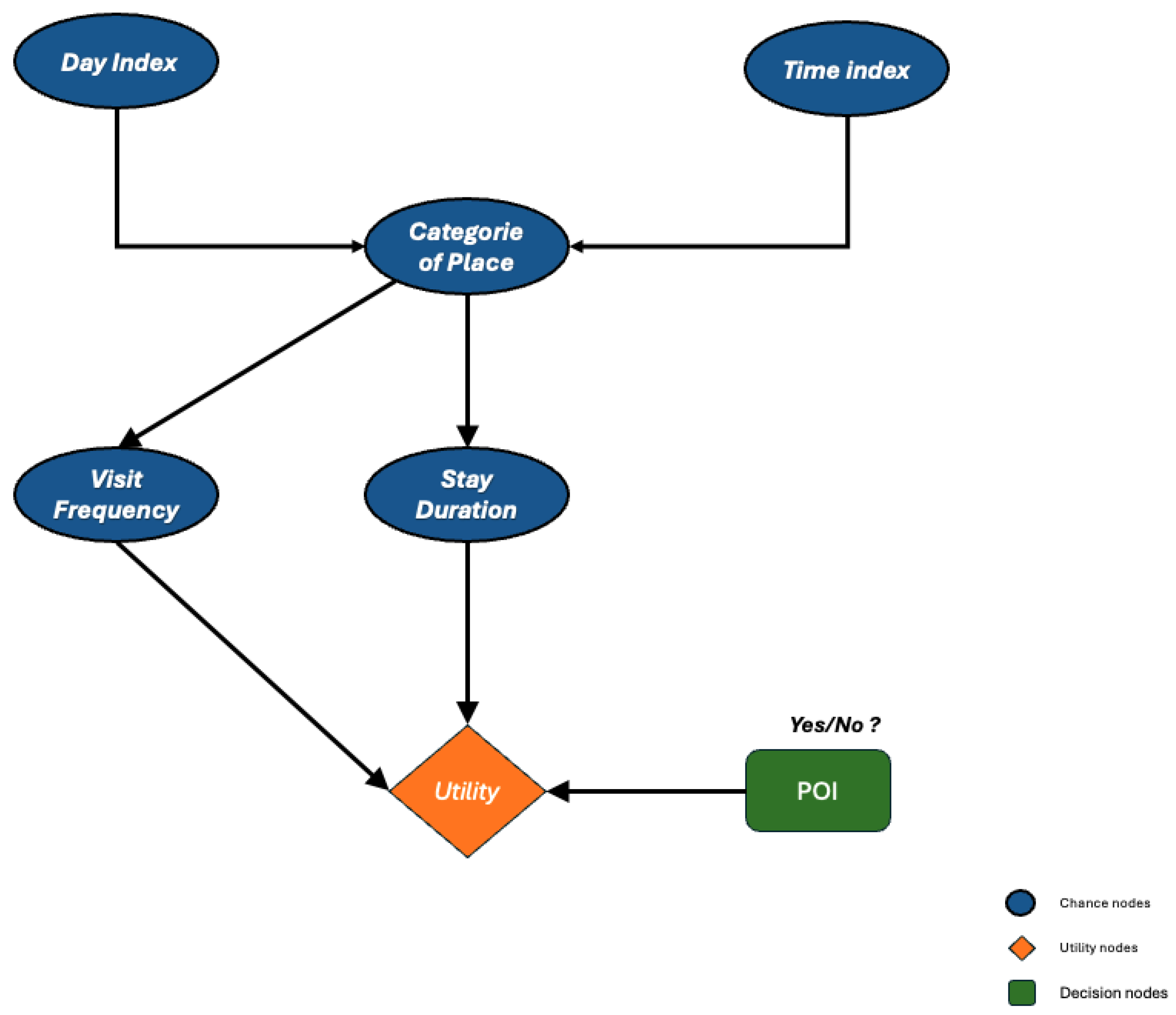
The structure of our Bayesian network, depicted in Figure 5, is designed to encapsulate and analyze user movement nuances from historical location data. It incorporates five variables: Day Index, Time Index, Category of Place, Visit Frequency, and Stay Duration.

The first two variables are crucial to reveal patterns in the frequency and timing of visits. They allow the network to discern daily and hourly trends, impacting where and when visits occur. The Day Index (represents the day of the week) can have values of 1, 2, or 3, respectively representing the following: daily distinctions, week weekend holiday categorizations, or no specific day distinction—with the number of possible values varying according to the level of distinction (seven for daily and three for grouped days). Time Index (represents the time of day) partitions the day into equal intervals such that a specific time like 08:31 would fall into a predetermined time slot, such as the fourth interval in a system where each interval spans two hours. We retrieve the Day Index and the Time Index into the vector W. These correspond to $td$ and $ts$, respectively. The variable Category of Place classifies locations into types such as restaurants, parks, or offices, evaluating their potential as POIs. The Visit Frequency measures how often a user returns to a particular location, providing insights into user preferences and routines, while Stay Duration gauges the length of each visit, offering clues about the site’s appeal or significance.

To categorize visit frequencies and average stay durations in G, we utilize Algorithm 3. This algorithm categorizes locations according to visit frequencies and stay durations within a user’s historical location graph G. We specify the number of categories k, such as three for low, medium, and high. In line 1, the input graph G is defined. In line 2, the number of categories k is set. The algorithm initializes dictionaries F and S to store visit frequencies and stay durations for each vertex (line 3). It iterates through each vertex v in the graph’s set of vertices $\mathcal{V}$ (line 4). For each weight tuple $\langle ts,td,fs,st\rangle$, the visit frequency $fs$ and stay duration $st$ are added to the dictionaries F and S for the vertex v (lines 7–9). After processing all vertices and edges, the algorithm computes quantiles for visit frequencies $Q_f$ and stay durations $Q_s$ using the function computeQuantiles (lines 10–11). It then iterates through each vertex v again (line 12) and each edge e where v is the source node (line 13). The weights for each edge are retrieved again (line 14). For each weight tuple, the algorithm determines the quantile category for the visit frequency and stay duration using getQuantileCategory (lines 15–16). Finally, the weight tuples are updated with these categories (line 17). The result is a categorized representation of locations based on visit frequencies and stay durations.

Algorithm 3. Categorization of locations according to visit frequencies and stay durations in G.

1: Input:  $G\leftarrow$ user’s mobility graph   2: Input:  $k\leftarrow$ number of categories (e.g., 3 for low, medium, high)   3: Initialize dictionaries F and S to store frequency and stay duration for each vertex   4: for each $v\in G.\mathcal{V}$ do   5:     for each $e\in G.\mathcal{E}$ where e is connected to v as the source node do ▹ For each edge connected to the vertex   6:         Retrieve $\mathcal{W}$ for edge e   7:         for each $\langle ts,td,fs,st,dt\rangle \in \mathcal{W}$ do   8:            $F\leftarrow F\cup fs$                 ▹ Add visit frequency   9:            $S\leftarrow S\cup st$                  ▹ Add stay duration 10:         end for 11:     end for 12: end for 13: $Q_f\leftarrow$ computeQuantiles(F, k)      ▹ Compute quantiles for frequency 14: $Q_s\leftarrow$ computeQuantiles(S, k)     ▹ Compute quantiles for stay duration 15: for each $v\in G.\mathcal{V}$ do 16:     for each $e\in G.\mathcal{E}$ where e is connected to v as the source node do 17:         Retrieve $\mathcal{W}$ for edge e 18:         for each $\langle ts,td,fs,st,dt\rangle \in \mathcal{W}$ do 19:            $fs\leftarrow \mathrm{getQuantileCategory}(fs,Q_f)$    ▹ Determine the position of the frequency fs as a function of its position relative to the quartiles Qf 20:            $st\leftarrow \mathrm{getQuantileCategory}(St,Q_s)$  ▹ Determine the position of the stay duration st as a function of its position relative to the quartiles Qs 21:            Update $\langle ts,td,fs,st,dt\rangle$ with $fs$ and $st$ 22:         end for 23:     end for 24: end for

These variables are interlinked within the network, where the Day Index and Time Index influence the Category of Place, which in turn affects both the Visit Frequency and the Stay Duration. This causality is represented in the network’s directed acyclic graph, which illustrates the directional influence of one variable over another, thereby structuring clear dynamics and dependencies within the model.

After defining this network structure, the next critical step involves configuring the network using historical data, which includes collecting comprehensive datasets and learning the CPTs for each node, except for the root nodes. These CPTs quantify how the states of parent nodes influence the states of their child nodes. The decision-making process within the network is facilitated by special nodes such as the Utility Node, which calculates the utility value based on the outputs from the Visit Frequency and Stay Duration. This utility reflects the desirability or value derived from visiting a specific category of place at certain times and frequencies, effectively guiding the decision on whether a location qualifies as a POI or not. The decision node (POI) evaluates whether the calculated utility exceeds a predefined threshold, indicating significant importance or interest, to decide about considering a location as a point of interest. The joint probability distribution of the network is given by the following:

$$\mathbb{P}(D,T,C,V,S)=\mathbb{P}\left(D\right)·\mathbb{P}(T\mid D)·\mathbb{P}(C\mid D,T)·\mathbb{P}(V\mid D,T,C)·\mathbb{P}(S\mid D,T,C,V)$$

(1)

where $\mathbb{P}\left(D\right)$ is the probability of the day; $\mathbb{P}(T\mid D)$ is the conditional probability of the time given the day; $\mathbb{P}(C\mid D,T)$ is the conditional probability of the category of place given the day and time; $\mathbb{P}(V\mid D,T,C)$ is the conditional probability of the visit frequency given the day, time, and category of place; and $\mathbb{P}(S\mid D,T,C,V)$ is the conditional probability of the stay duration given the day, time, category of place, and visit frequency.

By applying the property of conditional probability $\mathbb{P}(A,B)=\mathbb{P}\left(A\right)\mathbb{P}(B\mid A)$ and considering the conditional independence between the variables, we obtain the following assumptions:

• The day of the week D and the time T are independent of each other: $\mathbb{P}(T\mid D)=\mathbb{P}\left(T\right)$.
• The visit frequency V depends only on the category of place C: $\mathbb{P}(V\mid D,T,C)=\mathbb{P}(V\mid C)$.
• The stay duration S, given the category of place, is independent of $D,T$, and V: $\mathbb{P}(S\mid D,T,C,V)=\mathbb{P}(S\mid C)$.

Thus, the joint probability for this model, given the conditional independence assumptions, is as follows:

$$\mathbb{P}(D,T,C,V,S,P)=\mathbb{P}\left(D\right)\mathbb{P}\left(T\right)\mathbb{P}(C\mid D,T)\mathbb{P}(V\mid C)\mathbb{P}(S\mid C)$$

(2)

Algorithm 4 describes the construction of a Bayesian network from historical data. It takes as input a user’s mobility graph G and aims to produce a Bayesian network $bn$ with the constructed CPTs. In the first step, it calculates the basic probabilities for the day D and time T indices. It initializes counts for these indices and iterates through the nodes and edges of the graph G. For each edge connected to a source node, it retrieves the movement data $\mathcal{W}$ and increments the counts for the day and time indices based on the extracted values. Next, the algorithm calculates the conditional probabilities for each movement category C given the day and time indices. This involves aggregating the occurrences of each category and normalizing them to obtain the required probabilities. It also computes the conditional probabilities of variables V and S given C. These probabilities are essential for understanding the relationships between different variables within the network. In the third step, the algorithm constructs the CPTs for each node using the previously calculated probabilities: $\mathbb{P}\left(D\right)$, $\mathbb{P}\left(T\right)$, $\mathbb{P}(C\mid D,T)$, $\mathbb{P}(V\mid C)$, and $\mathbb{P}(S\mid C)$. This construction involves organizing the probabilities into a tabular format that represents the conditional dependencies between variables. These tables are crucial for the accurate functioning of the Bayesian network. Finally, it integrates the calculated CPTs into the corresponding nodes of the Bayesian network $bn$ and returns the completed network. This integration ensures that each node in the network is equipped with the necessary probabilistic information to perform inference.

Algorithm 4. Construction of a Bayesian Network from Historical Data.

1: Input:  G - user’s mobility graph   2: Output:  $bn$ - Bayesian network with constructed CPTs   3: Step 1: Calculation of Basic Probabilities ▹ Calculate the basic probabilities for day and time indices   4: Initialize counts for day index D and time index T   5: for each $v\in G.\mathcal{V}$ do   6:     for each $e\in G.\mathcal{E}$ where e is connected to v as the source node do   7:         Retrieve $\mathcal{W}$ for edge e   8:         for each $\langle ts,td,fs,st\rangle \in \mathcal{W}$ do   9:            Increment count of td and store in $coun{t}_d$ 10:            Increment count of ts and store in $coun{t}_t$ 11:         end for 12:     end for 13: end for 14: $\mathbb{P}(D=d)\leftarrow {\displaystyle \frac{coun{t}_d}{\mathrm{total}\mathrm{count}}}$; $\mathbb{P}(T=t)\leftarrow {\displaystyle \frac{coun{t}_t}{\mathrm{total}\mathrm{count}}}$ ▹ Compute the probabilities for day and time indices 15: Step 2: Calculation of Conditional Probabilities 16: $\mathbb{P}(C=category\mid D=td,T=ts)={\displaystyle \frac{\mathrm{count}(C=category,D=td,T=ts)}{\mathrm{count}(D=td,T=td)}}$ ▹ The probability of C given D and T 17: $\mathbb{P}(V\mid C=c)={\displaystyle \frac{\mathrm{count}(V,C=c)}{\mathrm{count}(C=c)}}$     ▹ Compute the probability of V given C 18: $\mathbb{P}(S\mid C=c)={\displaystyle \frac{\mathrm{count}(S,C=c)}{\mathrm{count}(C=c)}}$      ▹ Compute the probability of S given C 19: Step 3: Construction of the CPTs 20: Construct the CPTs for each node: 21:      $\mathbb{P}\left(D\right)$, $\mathbb{P}\left(T\right)$, $\mathbb{P}(C\mid D,T)$, $\mathbb{P}(V\mid C)$, $\mathbb{P}(S\mid C)$ ▹ Construct the CPTs for the nodes in the Bayesian Network 22: Step 4: Integration of the CPTs into the Network 23: Integrate the calculated CPTs into the corresponding nodes of the network $bn$ 24: Return  $bn$

4.5.3. POI Extraction Using the Bayesian Network

For the extraction of the POI, we have developed and implemented an algorithm based on a Bayesian network. This algorithm utilizes a probabilistic model to analyze and evaluate locations based on various attributes derived from users’ location histories. The goal is to determine whether a specific location can be classified as a POI, which is essential for constructing our mobility graph.

The Algorithm 5 extracts and evaluates the POIs using decision analysis and returns a reduced graph. The process begins by iterating through each vertex v in graph G. For each vertex, it retrieves the location metadata, specifically the “category”. It then examines each edge e connected to v as the source node and retrieves the weight $\mathcal{W}$ for the edge. For each tuple $\langle ts,td,fs,st\rangle$ in $\mathcal{W}$, the algorithm sets evidence in the Bayesian network with the elements $td,ts,fs,andst$. Using the Bayesian network, it identifies the posterior probabilities for the category, $fs$ and $st$, and computes the utility U based on the Bayesian network evidence and utilities. If the computed utility U meets or exceeds the threshold t, the vertex v is added to the reduced graph $G_{reduced}$. Subsequently, for each edge $e^{\prime }$ connected to v, if the edge $e^{\prime }$ is not already in the reduced graph, it assigns a weight $\langle ts,td,fs,st,dt\rangle$ to the edge. If the edge $e^{\prime }$ has contextual metadata, it associates these metadata using the function $f_m$. The edge $e^{\prime }$ is then added to the reduced graph $G_{reduced}$. The algorithm ensures that the weight of the relation $\langle ts,td,fs,st\rangle$ is updated if it already exists. Finally, the reduced graph $G_{reduced}$ is returned.

Algorithm 5. Reduced Graph Generation and Extraction of Points of Interest.

1: Input:  G - user’s mobility graph   2:     t - utility threshold   3:     $bn$ - Bayesian network (with decision node for POI)   4: Output:  $G_{reduced}$ - Reduced graph   5: Initialize an empty list $V_{selected}$ to store selected vertices   6: for each v in $G.V$ do   7:       $category\leftarrow$RetrieveLocationMetadataByName$(v,“\mathrm{category}”)$   8:       for each edge $e\in G.\mathcal{E}$ where e is connected to v as the source node do   9:          Retrieve $\mathcal{W}$ for edge e 10:          for each $\langle ts,td,fs,st\rangle$ in $\mathcal{W}$ do 11:             Set evidence in $bn$ with $td,ts,fs,st$ 12:             Identify posterior probabilities for category, $fs$ and $st$ using $bn$ 13:             Compute utility U based on $bn$ evidence and utilities 14:             if $U\ge t$ then ▹ Check if the computed utility meets or exceeds the threshold 15:                  $V_{selected}\leftarrow V_{selected}\cup \left\{v\right\}$ 16:             end if 17:          end for 18:     end for 19: end for   ▹ Construct $G_{reduced}$ by verifying relations between vertices in $V_{selected}$ 20: for each v in $V_{selected}$ do 21:       $G_{reduced}.\mathcal{V}\leftarrow G_{reduced}.\mathcal{V}\cup \left\{v\right\}$ 22:       for each edge $e^{\prime }\in G.\mathcal{E}$ where $e^{\prime }$ is connected to v do 23:          if target node of $e^{\prime }$ is in $V_{selected}$ and $e^{\prime }\notin G_{reduced}.\mathcal{E}$ then 24:             Assign $e^{\prime }$ weight $\langle ts,td,fs,st\rangle$ 25:             if $e^{\prime }$ has contextual metadata then 26:                  Associate $e^{\prime }$ with its contextual metadata using $f_m$ 27:             end if 28:             $G_{reduced}.\mathcal{E}\leftarrow G_{reduced}.\mathcal{E}\cup \left\{e^{\prime }\right\}$ 29:          end if 30:       end for 31: end for 32: return$G_{reduced}$                 ▹ Return the reduced graph

The utility function used to determine the desirability of a location as a POI is defined as follows:

$$\mathrm{Utility}=log\left(\mathbb{P}\right(C\mid D,T\left)\right)+log\left(\mathbb{P}\right(V\mid C\left)\right)+log\left(\mathbb{P}\right(S\mid C\left)\right)$$

(3)

This utility function is constructed using the logarithms of the conditional probabilities and helps to manage the range of probability values, as well as ensures that multiplying small probabilities does not result in extremely small utility values. By summing the logarithms of the probabilities, we effectively combine the influences of the Category of Place, Visit Frequency, and Stay Duration, capturing their combined impact on the decision-making process.

5. Experiments

We proceeded with the evaluation of the proposed method. Section 5.1 details the dataset used, the data collection procedures, and the evaluation metrics. Section 5.2 presents the experimental results, offering a comprehensive analysis and discussion of the findings.

5.1. Setting

5.1.1. Dataset Collection and Analysis

We have developed a cross-platform mobile application designed to collect GPS data from 10 volunteers who were willing to share their locations. Prior to data collection, each participant was provided with a detailed consent form outlining the types of data to be collected, the purpose of the research, and the steps taken to ensure that all collected data would be anonymized. The data were collected every 60 s, enabling us to monitor the movements and dwell times of participants across various locations over a period of 3 months. The total distance covered by these GPS logs exceeded 10,000 km. The collected data include timestamps and GPS coordinates, which provide essential information for constructing and evaluating the user mobility graph and the POI extraction algorithm.

All participants filled out and signed a consent form via https://form.jotform.com/242243188677566 (accessed on 1 March 2024) prior to the start of the study. This ensured that we had their official consent and provided them with detailed information on how their data would be used for the study. To ensure privacy, each participant was assigned a unique identifier via that was not linked to their personal information, making it impossible to trace the data back to an individual. Recognizing the inherent risk of re-identification with GPS data, we anonymized the information by rounding timestamps and obscuring specific location details that could potentially reveal a participant’s identity. Additionally, all data were encrypted to safeguard them from unauthorized access, ensuring that even if intercepted, they remained secure. Access to the raw data was strictly limited to authorized members of our research team, who were the only individuals permitted to handle the information.

Figure 6 displays a screenshot of the mobile application utilized for GPS data collection, while Figure 7 illustrates a sample of the distribution of collected GPS data points plotted on a map (The points on the map are too dense but do not represent paths).

Table 5. Statistics for dataset for evaluation.

Userid	N. of Track Points	Significant Location	Location Category	Distance Collect
001	83,491	90	15	2440.21 km
002	1205	12	4	74.68 km
003	37,011	56	33	2989.02 km
004	34,249	134	32	876.31 km
005	43,292	25	6	1412.42 km
006	13,298	112	9	1076.82 km
007	24,324	34	12	1989.23 km
008	32,424	102	21	489.38 km
009	42,032	56	11	2231.12 km
010	3923	20	7	54.28 km

displays the fundamental statistics of our dataset. The numbers from 01 to 10 in the first column represent the user IDs. The second column indicates the number of tuples collected. Column 3 details the categories of significant locations, while Column 4 lists the real POIs suggested by users. The final column shows the total distance of the collected data.

The occurrence of positioning errors in GPS loggers is a well-known issue, particularly in indoor environments [32]. Kjærgaard et al. [33] reported that even state-of-the-art GPS loggers experience positioning errors caused by environmental factors. Their findings showed that fewer than 80% of the track points in their experiments were within 20 m of the true locations. Our preliminary experiment revealed that similar errors occurred for track points obtained outside buildings. GPS positioning errors seem inevitable.

5.1.2. Parameter Selection

The

Table 6. Data preprocessing parameters for evaluation.

Parameter	Value
Time Threshold	5 min
Noise Reduction Window	10
Metadata API	Google Places API, OpenStreetMap
Unimportant Location	Road (e.g., highways, minor streets)

shows the data preprocessing parameters we used for the evaluation.

Table 7. POI extraction parameters.

Parameter	Value
Day Index	1 = Weekday, 2 = Weekend, 3 = Holiday
Time Index	1 = Morning, 2 = Afternoon, 3 = Night
Categorization for Stay Duration	Short, Medium, Long
Categorization for Visit Frequency	Low, Medium, High
Utility Threshold	−0.5, −0.75, −1

shows the parameters we used for reduced graph extraction. The categorization was performed using classification to determine short stay, long stay, and visit frequency categories.

The next step was to implement DJ cluster and then compare its results to our own novel POI extraction algorithm. We chose to implement DJ cluster because it offers superior results compared to other clustering approaches such as DBSCAN, DT cluster, k-means and TD cluster [34].

5.1.3. Evaluation Metrics

To evaluate the effectiveness of our POI extraction algorithm, we constructed a ground truth dataset using the GPS data collected from volunteers who shared their locations. This dataset was manually annotated with known points of interest, including their locations. If an extracted POI matched a true POI, we determined whether the predicted POI agreed with the true POI assignment. The prediction was categorized as a true positive ($T{P}_{POI}$) if it agreed with the ground truth label and as a false positive ($F{P}_{POI}$) otherwise. We classified any selected POI that did not match a true significant POI as a false positive. Additionally, we considered a true POI that was not matched by any selected POI as a false negative ($F{N}_{POI}$).

With $T{P}_{POI}$, $F{P}_{POI}$, and $F{N}_{POI}$, we commonly calculated the precision ($P_{POI}$) and recall ($R_{POI}$) scores as follows:

$$P_{POI}={\displaystyle \frac{T{P}_{POI}}{T{P}_{POI}+F{P}_{POI}}},R_{POI}={\displaystyle \frac{T{P}_{POI}}{T{P}_{POI}+F{N}_{POI}}}.$$

(4)

Then, the F1POI score was obtained by its harmonic mean:

$$F{1}_{POI}={\displaystyle \frac{2\times P_{POI}{R}_{POI}}{P_{POI}+R_{POI}}}={\displaystyle \frac{2\times T{P}_{POI}}{2\times T{P}_{POI}+F{N}_{POI}+F{P}_{POI}}}.$$

(5)

5.1.4. Complexity Analysis

We evaluated the reduced graph generation Algorithm 5 that was to be used to protect privacy. The total time complexity can be broken down into several key steps: the main loop that iterates over all vertices in the graph $O\left(n\right)$, nested loops that process the edges associated with each vertex $\left({\sum }_{i=0}^{n}i\right)=O\left(1\right)$, associated weights $O\left(k\right)$, and inferences in the Bayesian network $O\left(bn\right)$. The construction of the reduced graph adds an additional complexity of $O(n_s\times m)$. Therefore, the total complexity can be approximated as follows:

$$O(n\times k\times bn)+O\left(n_s\times m\right)$$

The complexity variables of the algorithm are as follows: n is the number of vertices in the graph G—determining the storage space for vertices; m is the number of edges in G—reflecting the space needed for edges and associated data; k is the number of weight tuples per edge—indicating data density; $bn$ represents the complexity of the Bayesian network inferences—impacting decision-making time; and $n_s$ is the number of selected vertices in the reduced graph $G_{reduced}$—influencing the size of the final graph. This formula indicates that the algorithm is primarily influenced by the size of the graph, data density, and the complexity of calculations within the Bayesian network.

The space complexity is primarily determined by the storage requirements for the vertices and edges in the graph, as well as the Bayesian network. The space complexity can be expressed as follows:

$$O(n+m+b{n}_{space})$$

where

• $b{n}_{space}$ is the space required to store the Bayesian network, reflecting the memory consumption of the inference model.

This complexity shows that memory usage grows linearly with the size of the graph and the complexity of the Bayesian network. While the algorithm is efficient in handling large graphs in terms of memory, the requirements could become significant in scenarios with extremely large or dense graphs, potentially leading to challenges in environments with limited storage capacity.

5.2. Experimental Results

Runtime performance experiments were carried out for the Reduced Graph Generation and the Points of Interest Extraction Algorithm 5, and the results, as illustrated in Figure 8, show significant variations among participants. These disparities in execution times may have arisen from differences in the underlying data or system performance. For our experimentation, we used a threshold of −0.75. The figure highlights that some users experienced considerably longer runtimes, indicating that their datasets or processes might have involved more complex or larger inputs, leading to extended execution times. A closer examination of the graph reveals a wide range of runtimes, with the shortest being nearly zero and the longest approaching 20 s. This variation could be attributed to differences in graph sizes or the complexity of the Bayesian inference process for each user. Additionally, the more POIs the algorithm detects, the more time it takes to build and search for POI connections in the reduced graph, which explains the longer execution times.

As illustrated in Figure 9, the precision for the threshold of −0.5 varied between 0.980 and 0.990, indicating high precision but with some variability among users. This variability can be attributed to differences in the quality of data among users. For example, some users may have had cleaner and better-labeled data, while others may have had noisier or poorly categorized data. By increasing the threshold to −0.75, the precision slightly decreased, ranging from 0.910 to 0.940. This could indicate that the model starts to trade-off between precision and recall, capturing more points of interest but with a slight decrease in precision. For the threshold of −1, the precision further decreased, fluctuating between 0.780 and 0.840. This drop in precision may have been due to an increase in false positives, where the model incorrectly identifies points of interest because of the reduced detection threshold.

Figure 9, Figure 10 and Figure 11 show, respectively, the precision, recall, and F1POI scores for three different thresholds −0.5, −0.75, and −1 across multiple users.

Figure 10 shows that recall is low for the −0.5 threshold, with values between 0.42 and 0.50. This poor recall performance suggests that the model failed to detect a large proportion of the points of interest. By increasing the threshold to −0.75, the recall improved significantly, ranging from 0.70 to 0.78. This improvement indicates that the model became more sensitive to the detection of points of interest, thus capturing a greater proportion of true points of interest. For the −1 threshold, the recall continued to show improvement, with values ranging from 0.80 to 0.88, although there is still considerable variability among users.

As illustrated in Figure 11, the F1POI score for the threshold of −0.5 varied significantly between 0.58 and 0.66, reflecting unstable model performance. It shows that, despite high precision, the low recall value pulled the F1POI score down. By increasing the threshold to −0.75, the F1POI score improved, with values ranging from 0.78 to 0.85, indicating better overall performance. This improvement in the F1POI score indicates a better balance between precision and recall, meaning that the model was more successful in correctly identifying points of interest while reducing detection errors. For the threshold of −1, the F1POI score is similar to that of the −0.75 threshold, ranging between 0.80 and 0.85, but it still showed significant fluctuations.

The results suggest that the −0.75 threshold offers a good compromise between precision and recall, providing a high F1POI score and better stability than the other thresholds. However, there is notable variability in performance between users. This variability is attributed to the quality of the data used to train and test the model. It is crucial to ensure that the identified locations are accurate and that the categories are correctly identified for the Bayesian network. Incorrect classification or inaccurate location data can greatly affect the model’s ability to infer correctly. The categories of points of interest must be consistent and correctly labeled to avoid confusion when constructing the Conditional Probability Tables. Additionally, the model identified points of interest with high precision, which is important for privacy due to the high probability calculated with the utility function.

We conducted experiments using the DJ cluster algorithm, testing it across a range of parameters to evaluate its performance. The parameters we varied include Eps (km) with values {0.01, 0.02, 0.05, 0.1, 0.2}, Merge distance (km) with values {0.02, 0.04, 0.1, 0.2, 0.4}, and Time shift (hours) with values {1, 2, 3, 4, 5, 6}. The goal was to observe how changes in these parameters would affect the algorithm’s ability to accurately identify POIs across multiple users.

The results, as depicted in the provided Figure 12, reveal that the DJ cluster algorithm demonstrated a moderate and inconsistent performance. When analyzing the precision across different users, we observed a range between 0.46 and 0.54. This variation indicates that while the algorithm can correctly identify true positives to some extent, its accuracy is inconsistent, leading to fluctuations in performance depending on the user data being analyzed. This inconsistency could be attributed to differences in the quality and structure of data across users, which may affect the algorithm’s ability to accurately cluster POI. The recall values, which measure the algorithm’s ability to capture all relevant POIs, are slightly more stable, ranging from 0.55 to 0.61. However, these values are still moderate, suggesting that the algorithm was missing a significant number of true positives. Despite the relative stability in recall, the moderate performance indicates that the DJ cluster algorithm may not be adequately sensitive to detect all relevant points of interest, which is critical in applications requiring comprehensive detection. The F-measure, which balances both precision and recall, fluctuated between 0.50 and 0.57 across the users. This fluctuation further underscores the variability in the algorithm’s performance. The F-measure is particularly important, as it reflects the overall effectiveness of the algorithm by considering both its precision and recall. The observed fluctuations suggest that while the algorithm might perform well in certain instances, it lacks consistency, which could undermine its reliability in practical applications. Overall, the performance of the DJ cluster algorithm, as illustrated in these graphs, indicates that while it can provide moderate results, its inconsistency across different users raises concerns about its robustness and generalizability. The significant variations in the precision, recall, and F-measure suggest that the algorithm may struggle with varying data qualities and complexities, leading to unreliable identification of points of interest in certain cases.

6. Discussion

Our method consistently outperformed the DJ Cluster algorithm across various thresholds, demonstrating higher and more stable values for precision, recall, and F-measure. This suggests that our approach is more reliable and effective in accurately identifying POIs while reducing detection errors. In contrast, the DJ cluster algorithm exhibited moderate and inconsistent performance, with significant fluctuations in its precision and F-measure values, indicating varying accuracy in identifying true positives. The results highlight that our method strikes a better balance between precision and recall, leading to higher F1POI scores, which suggests superior overall performance. This balance is crucial for ensuring that the model not only identifies POIs with high precision but also captures a significant proportion of true POIs, thereby enhancing its robustness and reliability. In summary, while the DJ cluster algorithm may perform adequately under certain conditions, our approach offers a more dependable solution for clustering tasks, particularly in scenarios requiring precise and reliable identification of POIs.

7. Conclusions

In this paper, we proposed a user mobility model based on graphs for crowdsourcing applications, which we have formalized and enhanced with an advanced algorithm for identifying POIs. The advantage of the graph-based formalism lies in its ability to represent paths and relationships between POIs in a structured and dynamic manner, facilitating the analysis of user mobility patterns. This graphical representation allows for the clear visualization and efficient manipulation of mobility data, thereby improving the accuracy of movement predictions and privacy protection measures. By integrating Bayesian networks, we have introduced a model to effectively identify significant POIs. The Bayesian network can model and calculate the joint probability that a specific location is a POI, taking into account several important factors, including the day of the week, the time of day, the category of the place, the frequency of visits, and the duration of each stay. The limitation of this paper lies in the need to improve the quality of the location data with the corresponding categories to enable the model to accurately infer POIs. Our preliminary experiments have shown that similar errors occur with track points obtained outside buildings, with GPS positioning errors appearing to be inevitable. Given our focus on privacy protection and the necessity for high-quality data, these limitations highlight the importance of considering additional factors in future work. Specifically, we plan to incorporate the user’s profile, time period, and the category of nearby locations to better estimate the user’s location. For instance, if a user has a student profile, our system would prioritize locations such as libraries, lecture halls, and university campuses within a certain radius and during specific times of the day. By enhancing the precision and relevance of mobility predictions, our approach aims to further strengthen privacy protection against inference attacks. Future research will focus on refining the model to improve data quality, ensuring that the model can infer POIs with a higher F1POI score. These efforts will better protect sensitive user information in crowdsourcing environments against inference attacks, taking into account the contextual information that an attacker might possess.